Educational Grants Closing the Gap in Schooling Attainment

between Poor and Non-Poor

Melanie RaymondEconomic Studies and Policy Analysis Division

Department of Finance, Canadaand

Elisabeth SadouletDepartment of Agricultural and Resource Economics

University of California - Berkeley ∗

First draft: April 2002This version: May 2003

Abstract

The present work assesses the effectiveness of educational grants at raising schooling attain-ment of poor children in rural areas. The per grade gains in reducing drop outs cumulate in anadditional half a year in total schooling. Progressive impacts are found along three dimensions:degree of poverty, parents’ education and distance to school. The children of uneducated fathersliving far from school gain twice as much as their counterparts with an educated father or closeto a school. The intervention successfully closes the schooling gap along the wealth dimensionbut falls short of achieving the same in the other dimensions of parents’ education and schooldistance.

1 Introduction

Education has long been recognized as a key weapon in fighting poverty, especially in developingcountries. Hence governments and international development agencies have promoted policies thatenhance educational achievement. Many such policies have focused on the lack or low quality of ser-vices, which are found to disproportionately affect poor children (Behrman and Knowles 1999, Al-derman, Orazem and Paterno 2001). Initiatives encourage private sector involvement, like thePakistani Quetta program (Kim, Alderman and Orazem 1999) and voucher programs in Colombia

∗Special thanks go to Erin McCormick and Renos Vakis. This work would not have been possible without theprecious help of the PROGRESA team in Mexico which provided us with the data and insight about the workings ofthe program. The authors benefited from discussions with and suggestions from Gabriel Desmombynes, Pierre Duboisand Antoine Bommier. Thanks also go to seminar participants at the University of California, Berkeley, and at theUniversity of Syracuse for helpful comments. Early version was presented at the Annual Meetings of the AmericanAgricultural Economics Association in Chicago, August 2001. Melanie Raymond appreciated financial support fromthe Social Sciences and Humanities Research Council of Canada. Previously circulated under “Educational GrantsClosing the Gap in Schooling Attainment between Poor and non-Poor”.

(Angrist, Bettinger, Bloom, King and Kremer 2002), Bangladesh, Belize and Lesotho (West 1997).Programs address problems with teachers’ training, their attendance, school infrastructures, furni-ture, textbook availability and library resources. The Mexican Pare Program, in 1992-1997, is anexample of provision of school inputs that successfully improved the students’ schooling attainment(Lopez-Acevedo 1999).

A recent wave of programs took the issue from the demand side, encouraging parents to sendtheir kids to school with conditional cash or food transfer programs. In 1997, the Mexican govern-ment launched the Progresa program that offers grants to rural poor for primary and secondaryschooling. Similar programs were developed in Honduras, Nicaragua, Brazil. Other programs suchas the Food for Education in Bangladesh offers in kind transfers to parents sending their childrento school.

The premises for the success of such programs is that the supply of school is sufficiently adequate,and that the main barriers to schooling come from income constraints, direct costs, opportunitycosts, as well as preferences. The heterogeneity of the poor households with respect to thesecharacteristics presumes heterogeneity in impact of a cash transfer program. The present studyassesses the Mexican program Progresa, and focuses on its impact on schooling attainment for avariety of clienteles. This impact analysis is based on a model of schooling attainment decision thathighlights the determinants of school attainment across an heterogenous population (Bommier andLambert 2000, Binder 1998, Tansel 1997, Akhtar 1996, Lillard and Willis 1994). The randomizationof program beneficiaries in the sample of households selected for the program evaluation allows aclear identification of the program impact.

The current work complements assessments done of Progresa by Skoufias and Parker (2001),Schultz (2001) and Behrman, Sengupta and Todd (2001). Behrman et al study the average impacton the process of schooling including the entry age, grade repetition, dropout rates and schoolreentry rates. Schultz, on the other hand, offers disaggregate evidence by grade and gender onenrolments and evaluates the internal rate of return of the program. Finally, Skoufias and Parkerinvestigate the potential of school grants for reducing child labor participation.

The three dimensions of heterogeneity that we study - degree of poverty, education of theparents and the proximity of a school - particularly matter for poor families. The high incomeelasticity of school has been documented by Behrman and Knowles (1999). Conditional transfersare however similar to a price subsidy, and hence their effect entails a substitution effect in additionto the income effect. There is, to our knowledge, no empirical studies of price elasticities for school.Poorly educated parents tend to invest less in their children. If low earnings are the root cause ofthe lower educational outcomes, then looking at differential impact by educational level of parents isequivalent to studying the impact by poverty level. If less educated parents have lower preferencesor illiteracy handicap, the gains across parents’ education levels may exhibit a very different patternthan across degrees of poverty.

Finally, families not served by a school in their community face a higher cost than other familiesto sending their children to school (Handa 2002, Lavy 1996). Low or no access to public services isanother dimension of poverty. A price subsidy in the form of conditional transfer directly addressesthe cost issue.

2

We find that the Mexican grant program succeeds, on average, to increase the schooling attain-ment of the poor by a little more than half of a ten-month school year, from 6.8 years to 7.4 years.Children from families facing the greatest barriers - the poorest of the poor, uneducated parentsand living in a community not served by a high school - gain most from the program. Hence, theprogram has a progressive impact along all three dimensions. Furthermore, and most importantly,the grants succeed at closing the gap in schooling attainment between poor and non-poor.

The paper is organized as follows: we first describe the Progresa program and the schooling sit-uation in Mexico. Section 3 presents a dynamic model of schooling attainment and its econometricimplementation. We present the data used and discuss the impact measurement in the empiricalstrategy section. Results are then presented and policy considerations are discussed in sections 5and 6.

2 The Mexican Cash Transfer Program Progresa

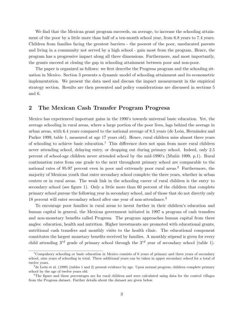
Mexico has experienced important gains in the 1990’s towards universal basic education. Yet, theaverage schooling in rural areas, where a large portion of the poor lives, lags behind the average inurban areas, with 6.4 years compared to the national average of 8.5 years (de Leon, Hernandez andParker 1999, table 1, measured at age 17 years old). Hence, rural children miss almost three yearsof schooling to achieve basic education.1 This difference does not span from more rural childrennever attending school, delaying entry, or dropping out during primary school. Indeed, only 2.5percent of school-age children never attended school by the mid-1990’s (Muniz 1999, p.1). Ruralcontinuation rates from one grade to the next throughout primary school are comparable to thenational rates of 95-97 percent even in poor and extremely poor rural areas.2 Furthermore, themajority of Mexican youth that enter secondary school complete the three years, whether in urbancenters or in rural areas. The weak link in the schooling career of rural children is the entry tosecondary school (see figure 1). Only a little more than 60 percent of the children that completeprimary school pursue the following year in secondary school, and of those that do not directly only18 percent will enter secondary school after one year of non-attendance.3

To encourage poor families in rural areas to invest further in their children’s education andhuman capital in general, the Mexican government initiated in 1997 a program of cash transfersand non-monetary benefits called Progresa. The program approaches human capital from threeangles: education, health and nutrition. Higher investments are promoted with educational grants,nutritional cash transfers and monthly visits to the health clinic. The educational componentconstitutes the largest monetary benefits received by families. A monthly stipend is given for everychild attending 3rd grade of primary school through the 3rd year of secondary school (table 1).

1Compulsory schooling or basic education in Mexico consists of 6 years of primary and three years of secondaryschool, nine years of schooling in total. Three additional years can be taken in upper secondary school for a total oftwelve years.

2de Leon et al. (1999) (tables 1 and 2) present evidence by age. Upon normal progress, children complete primaryschool by the age of twelve years old.

3The figure and these percentages are for rural children and were calculated using data for the control villagesfrom the Progresa dataset. Further details about the dataset are given below.

3

The benefits increase with each grade with a large increase between primary and secondary school. They are also slightly higher for girls than for boys in secondary school. The grants are paidto the mother of the family every two months, conditional on a minimum attendance of 85% ofschool days per month. The program also provides an amount for school supplies at the beginningof every school year. The value of the per family grant was capped at 790 pesos or about $90 permonth in January 2000.

Combined with the health intervention that promotes good health and nutritional status, Pro-gresa benefits can induce higher primary school completion by reducing the drop-out rate eachyear, and enable more teenagers to pursue their schooling at the secondary school level. Thesecumulated impacts should increase the schooling attainment in rural Mexico and the proportion ofchildren that complete basic schooling. The program has grown to include 2.6 million families in2000,4 and the benefits represent an average of 22 percent of the recipient families’ income. Theextent and the importance of the benefits to the beneficiaries makes the program one of the largestcash transfers programs in a developing country, with a budget totaling 0.2% of the Mexican GDP.

3 Schooling: Result of Sequential Decisions

3.1 Theoretical Framework

Schooling attainment is the result of a series of sequential enrollment decisions. Parents5 decideto enroll their child in primary school for the first time with some desired or optimal length ofschooling in mind. As the child progresses, parents must reiterate the enrollment decision everyyear until the optimal level of schooling is attained. While considering the current enrollment oftheir child, parents update their valuation for schooling and its corresponding desired level. Dueto this updating, the optimal schooling may change as the child progresses through school.

Consider a child that has completed g grades. By enrolling the child in grade g + 1, the familyanticipates benefits and costs associated with the extra year of schooling. The benefits here referspecifically to cash transfers to families. In addition, attendance of the extra grade gives access tofurther schooling to the child upon his success of the current grade. Thereby, the discounted valueof future schooling adds to the net benefits of enrolling in g + 1. The full benefit associated withenrolling in grade g +1 is thus: Tg+1−Cg+1 + βV (g +1) where Tg+1 is the transfer, Cg+1 the cost,and V (g + 1) the value function of having obtained grade g + 1 discounted by the time preferencerate β.

On the other hand, the child can start working and earn wages associated with his completedschooling and his individual characteristics Z, for the rest of his working life. In this instance, theutility of not enrolling the child is the present value of lifetime earnings: w(g;Z)

1−β .The value function for grade g takes the highest value between continuing school and starting

to work. The following Bellman equation expresses this value upon which enrollment decision is

4Extended in 2002 to cover six years of secondary school and to include small cities, the program bears now thename of Opportunidades.

5We abstract from the consideration of intra-household sharing of the decisions, notably with the child, and called“parents” the decision-maker.

4

made:

V (g) = max{

Tg+1 − Cg+1 + βV (g + 1),w(g; Z)1− β

}. (1)

Let Eg+1 represent the enrollment decision for grade g + 1. Then:

Eg+1 =

1 if Tg+1 − Cg+1 + βV (g + 1) ≥ w(g;Z)1−β

0 if Tg+1 − Cg+1 + βV (g + 1) < w(g;Z)1−β

conditional on Ek = 1 ∀k = 1, . . . , g. (2)

Parents will terminate their investment in the child’s schooling when the present net benefit ofan additional year of schooling is lower than the present value of the achieved schooling: Tg+1 −Cg+1 + βV (g + 1) 6 w(g;Z)

1−β or V (g) = w(g;Z)1−β .

Assuming away reentry after a temporary absence of one or more years from school, schoolingattainment is defined to be the last grade completed upon failure to enroll.

3.2 Econometric Implementation

The event that schooling attainment G takes the value g is equivalent to the event that the childdrops out of school after achieving g grades. From the standpoint of the econometrician thatimperfectly observes the elements of the enrollment process, the decision in equation 2 becomesstochastic with the addition of an error term, and leads to the conditional probability of observinga failure to enroll. Thus, the probability of failing to enroll in g + 1 matches the probability ofattaining g years of schooling, conditional on past enrollment decisions:

Pr(Eg+1 = 0|Ek = 1 ∀k = 1, . . . , g) =Pr(G = g)Pr(G > g)

= λ(g + 1). (3)

This expression corresponds to the risk or hazard rate of dropping out of school after havingcompleted grade g and before the completion of grade g + 1, given that the child has continuouslybeen in school up to the g + 1 enrollment time.6

We use a proportional hazard duration model to estimate these conditional probabilities andto assess the impact of Progresa on the risk of drop-out and schooling attainment. Durationmodels fit the dynamic nature of the schooling attainment decision, while the proportional modelsimpose a minimum of assumptions about the shape of the risk. Proportional models postulatethat individual hazard rate λ for individual i at grade g + 1 are proportional to a baseline hazardrate λ0(g + 1) such that: λi(g + 1) = λ0(g + 1)µi. The baseline hazard rate can be thoughtas being the common risk of dropping out in the population. Common beliefs, such as culturalbeliefs about the importance of schooling, and general labor conditions enter this common risk ofdropping out. Rather than attempting to model this common risk, proportional hazard models

6Schooling attainment has the particularity that if you “exit” during grade g + 1, it takes the value g. Tostatistically satisfy this characteristic, the event is to drop-out after grade g which exactly corresponds to the failureof enrolling in g + 1 at the beginning of the school year.

5

take a non-parametric approach, i.e. estimate independent values for all grades.The proportion µi by which the individual rate differs from the average, is determined by some

function of the individual’s covariates. We assume that the data generating process takes the formof an exponential function such that µi = exp(Xiβ). This specification makes µi nonnegative,which has the advantage of not imposing restrictions on β.7 The individual hazard rate for gradeg is thus: λi(g + 1) = λ0(g + 1) exp(Xiβ) where Xi is a vector of covariates for observation i.

Following the decision rule (equation 2), the hazard rate is a function of the transfer T , thecosts C, the wage w(g; Z) for the schooling completed and individual characteristics that influenceit, and the discount rate β - included in the vector of individual characteristics Xi in the hazardrate. The value function at the next higher grade V (g + 1) is unobserved and thus, is incorporatedin the error term. The hazard rate can thus be written as:

λ(g + 1) = λ0(g + 1) exp(αTg+1 + γCg+1 + δw(g; Z) + θβ + σZ). (4)

The hazard rates will be estimated following the Cox method. Cox proportional hazard model isa semi-parametric method that estimates parametrically the influence of individual characteristics,and estimates non-parametrically the baseline of the hazard ratio.

4 Empirical Strategy

To estimate the impact of educational grants on schooling attainment, the impact is first capturedon the drop-out rates for each grade. Using the predicted hazard rates, the schooling attainment isthen computed. Our empirical strategy makes use of the quasi-experimental nature of the Progresadata to measure the impact. The next section explains the data source and its quasi-experimentalstructure and how this advantage is exploited. The following section discusses the variables includedin the analysis.

4.1 Assessing the Impact on Drop-Out Rates and Schooling

The National Direction of Progresa had evaluation goals and made use of implementation con-straints to create a quasi-experimental dataset. The geographic coverage and size of the targetedbeneficiary population made it impossible to initiate the program simultaneously throughout thecountry. A phase-in implementation approach was used and allowed to create a control group.

The program devised a two-step targeting mechanism to identify beneficiaries. First, the Di-rection identified localities with high levels of poverty where the program would be offered. Thecriterion was the degree of marginality of all the localities in rural areas,8 as computed on thebasis of welfare indicators collected through population census by the Mexican government. Thisindicator also determined the timing of their incorporation of the villages into the program. Then,using census data from the selected villages, the eligible households were identified on the basis

7Kiefer (1988), p.664.8Localities are defined as rural if their population is below 2,500 inhabitants. For services accessibility concerns,

localities of less than 50 inhabitants were excluded.

6

of a discriminant analysis of income and other poverty considerations like dependency ratio anddwelling qualities. Households were characterized as poor and therefore eligible, or non-poor andnon-eligible.

To build the experimental sample for the evaluation purpose, a subset of 506 localities in sevenstates from the same incorporation round was drawn from the pool of localities identified as programrecipients. Incorporation was delayed by two years for a third of these localities. They constitutethe control villages and were randomly assigned to the later date of incorporation. We call Progresavillages the group of “on-time incorporated” localities and non-Progresa villages the group of the“incorporated with delay” localities. The outcomes of the eligible families in Progresa villages -the treated group - can thus be compared to those of eligible families in non-Progresa villages -the control group - to assess the impact of the program.9 We concentrate on the impact of beingeligible as opposed to being treated. The intention-to-treat effect is in the present case close to thetreatment effect since the number of eligible but non-participant households is small, less than 5%.Hence, we drop the distinction between intention-to-treat and treatment effect in the rest of thetext.

Making use of the quasi-experimental nature of the data, the Progresa transfers T in equation 4are represented using a set of dummies. First, a dummy Pv indicates the type of village (Progresaor not), and a second one ei the type of family (poor and thus eligible or not) the child comesfrom. A set of dummies indicates the grade g + 1 the child will enter, for the grades primary 3 tosecondary 3, that is dh,g+1 = 1 if h = g + 1 and 0 otherwise where h ∈ [3, 9]. The product of thesedummies captures the grade specific effect of Progresa. Including these indicator variables andletting the costs, wage, personal characteristics and discount factor enter Xg+1 = [Cg+1, w, Z, β],the hazard rate for child i in village v (equation 4) becomes:

λiv(g + 1) = λ0(g + 1) exp

(α1Pv + α2ei +

9∑

h=3

γhdh,g+1eiPv + Xi,g+1α3

), (5)

where dh,g+1eiPv ≡ Tg+1. The γh’s capture the impact of the child’s eligibility for receiving benefitsfor grade h on the drop-out rate in grade three (primary 3) through nine (secondary 3).10

Furthermore, an interaction term for wealth and the grants is included to assess how grantseffectively counter the effect of poverty on schooling outcomes. For ease of interpretation, thewealth index is introduced for poor and non-poor separately as Y p and Y np in equation 5:

λiv(g + 1) = λ0(g + 1) exp

(α1Pv + α2ei +

9∑

h=3

(γh + ζY pi )dh,g+1eiPv + δ1Y

npi + δ2Y

pi + Xi,g+1α3

). (6)

The influence of wealth on the decision to continue school is captured with the three parameters

9Behrman and Todd (1999) verify the comparability of the treatment and the control groups on the basis ofpre-program characteristics and outcomes. They find that the control group is similar in multiple dimensions to thetreatment group.

10By adding γ1 and γ2, the model can capture the anticipation effect the program may have on drop-out rates forthese two grades. The possibility of anticipation effects was explored empirically and will be discussed in the resultssection.

7

δ1, δ2 and ζ. The parameter δ1 measures the role of relative wealth within the group of non-poor households, δ2 measures the role of wealth among the poor households that are not in thetreatment area, while δ2 + ζ measures the role of wealth among the poor that can benefit fromthe grants. Both parameters δ1 and δ2 are expected to be positive as children from wealthierhouseholds are expected to have a higher probability to continue school. This specification allowsto test whether the grant program can counteract the poverty handicap among the poor by testingfor the hypothesis H0 : δ2 = ζ.

To compute the schooling attainment from the survival model, drop-out risks are computed forall children and then averaged by grade. These average drop-out risks can be used to calculate theexpected schooling attainment as follows:

E[G] =K∑

g=1

g Pr(G = g) =K∑

g=1

g

g∏

k=1

(1− λk), (7)

which can be rewritten as:

E[G] = 1 +K∑

g=1

(g∏

k=1

(1− λk)

). (8)

The schooling attainment for treated and control children are computed separately and thedifference between the two groups gives the program impact.

4.2 Determinants of the Drop-out Rate

The present work draws data from the baseline survey (Encaseh) of November 1997 and the evalu-ation surveys (Encel) of October 1998 and November 1999. The surveys contain detailed informa-tion about each household member as well as household characteristics for 11,000 households withschool-aged children.

We use information about adults’ occupation along with the average level of schooling in the vil-lage and the distance to the capital to capture off-farm earning potential in the school continuationequation above (equation 2). On-farm labor needs are characterized by the household’s agriculturalassets, while demand for caring for younger siblings is captured by the number of children 0 to 5years old. Both agricultural assets and the number of young siblings vary over time. We furtherinclude age dummies, gender and work experience in the previous year to capture the child’s workopportunities.

Glewwe and Jacoby (1994) suggest that individual characteristics, such as ability, and familyfactors, such as parental education, affect the child’s learning productivity and thus the earningspotential of the child. To account for learning productivity, the entry age to primary school, andgrade failure in the previous year are included in Z. To proxy for schooling progress, the age isused within grade groups: for grades 1 to 3, for grades 4 to 6 and for grades 7 to 9. The humancapital of the parents also influence the learning productivity, either due to higher preferences orhigher earnings. These additional dimensions of learning productivity are proxied by the education

8

of parents, as well as their ethnicity (to allow preference differences across ethnicity).The costs of schooling Cg+1 for Mexican families are mainly travel costs, as schools are free and

uniforms are generally not required. Since the program is offered in villages that have a primaryschool, there is no travel cost for this level. Only the distance to secondary school is included tocapture costs of schooling for children considering an enrollment decision at the secondary schoollevel.

Finally, the discount factor is influenced by the family’s wealth and capacity to face the costsand opportunity costs of schooling, especially if there are market imperfections limiting the family’sability to borrow against the child’s future earnings. The percentiles of the wealth index11 calculatedby the program direction to identify the poor families is included. The number of children in ageto attend primary and secondary school are also included separately. The latter will capture thetotal schooling costs the family faces. The sample for this study counts 20,541 children betweenthe age of 5 and 16 years old and include only children that were enrolled in 1997 and whose twoparents were living at home12, .

5 Results

5.1 Impact on the Drop-Out Rates

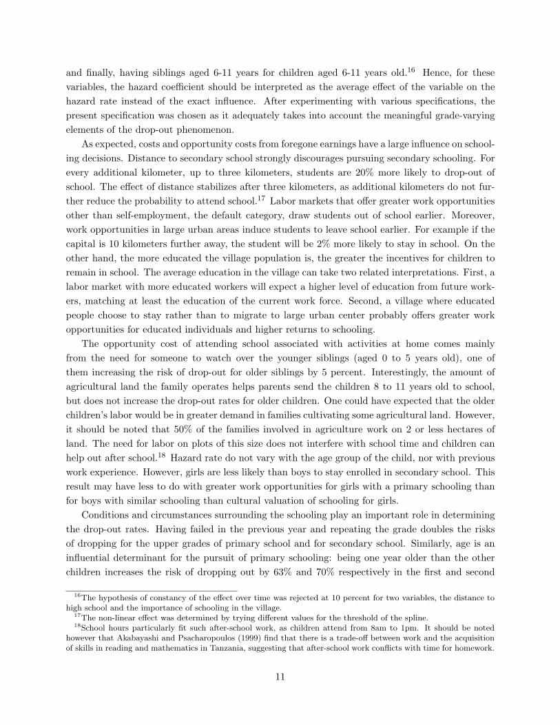
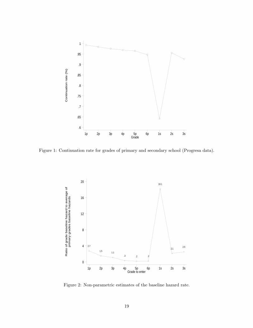
The drop-out risk is estimated using a Cox proportional hazard model with the baseline hazardbeing estimated non-parametrically. The estimation results are presented in table 2 with the non-parametric estimates of the baseline hazard λ0(g) depicted in figure 2. The figure presents therelative baseline hazard rate (normalized by the average hazard rate for primary school grades)for all six grades of primary school (labeled 1p to 6p) and the three grades of secondary school(labeled 1s to 3s). The graph echoes earlier observations, that the risk of dropping out is largestat the entry of secondary school. The risk at that moment, 1s in the figure, is 18 times greaterthan the average risk from primary grades and 7 to 9 times larger than the risks in higher gradesof secondary school. The baseline risk is also higher for the rest of secondary school relative toprimary school.

When and by how much do educational grants alter the drop-out decision? Table 2 presentsthe results of the hazard rate estimation. It gives the relative hazard ratio associated with eachvariable, which is eθ rather than the estimated parameter θ. The hazard ratio tells by how muchthe independent variable alters the probability of dropping out of school. For example, the relative

11The wealth index used is the initial index constructed by the Progresa Direction to identify the eligible families.The discriminant analysis included family composition, income and assets, and dwellings characteristics. The valueof the index itself cannot be directly interpreted as the dollar value of the family’s wealth. It only offers a relativeranking of the families. Hence, we choose to use percentiles of this index to ease the interpretation of the results.Furthermore, the wealth index does not perfectly correspond to the final classification of eligibility of families sincethere was a process of local adjustment of the list of beneficiaries. Thus, the percentiles of wealth can be included inthe regression along with the dummy to identify the eligible families without introducing problems of multicolinearity.

12We chose to ignore the cases where either the father, the mother or both were absent from the household, as thecharacteristics of the absent parent such as his education are missing.

9

hazard ratio corresponding to being from an eligible family is 1.56, indicating that the probabilityto drop-out when being poor is 56% of what it would be if being non-poor.

The results reveal that Progresa grants significantly attenuate the risk of dropping out for all theeligible grades (table 2, variables ”Treatment effects” in the second half of the table). For example,Progresa decreases drop-outs at the entry to secondary school by 45 percent from the baselineλ0(1s). Applied to the average continuation rate described in figure 1, this would approximatelyraise the continuation rate into secondary school from 63% to 80%. In the overall, the grants reducethe risk of dropping out for all grades by 40 to 54%. Although the point estimate is lower for thefirst two grades, none of these effects are significantly different from each other.

The model was also estimated to account for possible anticipation effects of the program (resultsnot presented here). Parents may be influenced in their decisions for first and second grades,knowing that the child will be eligible for grants starting in third grade. No effect was found.13

This lack of anticipation effect may be due to the initial announcement that the eligibility of thefamilies would last three years and then be re-evaluated.

The basic drop-out pattern, the baseline hazard rate, does not vary between 1998 and 1999as indicated by the year 1998 dummy (table 2). One could imagine that the program may havea stronger impact the first year of its implementation than in the following years. To test if thishypothesis is true, an average time impact was added to equation 4 in the form of γ98t98eiPv whereγ98 captures the differential impact between the first year of the program and the following one(results not reported). This varying average impact was rejected at 95%. We also checked for apotential first year impact by grade, by adding

∑9h=3 γ98

h t98dg,h+1eiPv in equation 4 (results notreported). Once again, the tests rejected time-varying impact of the transfers for all the gradesexcept the second grade of secondary school.14

As discussed in section 4.2, some covariates may influence the drop-out risk differently acrossgrades, levels or age groups. To determine whether a covariate should vary in any of these threedimensions, several specifications were estimated and tested.15 The proportional hazard modelassumes that the influence of individual characteristics on the hazard is constant over grade. Forexample, the family owes a business increases the hazard by 6%, the proportional hazard modelimplies that the family asset effect is constant throughout schooling. The test verifies the validityof this assumption for each covariate and for the overall specification. Only the overall specificationtest is reported at the bottom of the table. The hypothesis of constant effect cannot be rejectedfor the overall specification, and for all the individual variables except five including being 12 yearsold or older, having failed a grade between grades 4 and 6 in primary school and between grades1 and 3 in secondary school (included as two separate factors), the birth order in primary school

13Behrman et al. (2001) found evidence of less grade repetition throughout the primary school grades, includingin first and second grades. Thus, parents may not choose to have their children start early as a consequence of thegrants, but once children are in first and second grades, they may monitor more closely their progress.

14The effect for the secondary 2 over the two years becomes insignificant, and only the effect for the first year issignificant, decreasing the drop-out risk by 50 percent. Since the results are almost identical to the ones presented intable 2, these results are not included.

15The test follows a generalization of Grambsch and Therneau (1994).

10

and finally, having siblings aged 6-11 years for children aged 6-11 years old.16 Hence, for thesevariables, the hazard coefficient should be interpreted as the average effect of the variable on thehazard rate instead of the exact influence. After experimenting with various specifications, thepresent specification was chosen as it adequately takes into account the meaningful grade-varyingelements of the drop-out phenomenon.

As expected, costs and opportunity costs from foregone earnings have a large influence on school-ing decisions. Distance to secondary school strongly discourages pursuing secondary schooling. Forevery additional kilometer, up to three kilometers, students are 20% more likely to drop-out ofschool. The effect of distance stabilizes after three kilometers, as additional kilometers do not fur-ther reduce the probability to attend school.17 Labor markets that offer greater work opportunitiesother than self-employment, the default category, draw students out of school earlier. Moreover,work opportunities in large urban areas induce students to leave school earlier. For example if thecapital is 10 kilometers further away, the student will be 2% more likely to stay in school. On theother hand, the more educated the village population is, the greater the incentives for children toremain in school. The average education in the village can take two related interpretations. First, alabor market with more educated workers will expect a higher level of education from future work-ers, matching at least the education of the current work force. Second, a village where educatedpeople choose to stay rather than to migrate to large urban center probably offers greater workopportunities for educated individuals and higher returns to schooling.

The opportunity cost of attending school associated with activities at home comes mainlyfrom the need for someone to watch over the younger siblings (aged 0 to 5 years old), one ofthem increasing the risk of drop-out for older siblings by 5 percent. Interestingly, the amount ofagricultural land the family operates helps parents send the children 8 to 11 years old to school,but does not increase the drop-out rates for older children. One could have expected that the olderchildren’s labor would be in greater demand in families cultivating some agricultural land. However,it should be noted that 50% of the families involved in agriculture work on 2 or less hectares ofland. The need for labor on plots of this size does not interfere with school time and children canhelp out after school.18 Hazard rate do not vary with the age group of the child, nor with previouswork experience. However, girls are less likely than boys to stay enrolled in secondary school. Thisresult may have less to do with greater work opportunities for girls with a primary schooling thanfor boys with similar schooling than cultural valuation of schooling for girls.

Conditions and circumstances surrounding the schooling play an important role in determiningthe drop-out rates. Having failed in the previous year and repeating the grade doubles the risksof dropping for the upper grades of primary school and for secondary school. Similarly, age is aninfluential determinant for the pursuit of primary schooling: being one year older than the otherchildren increases the risk of dropping out by 63% and 70% respectively in the first and second

16The hypothesis of constancy of the effect over time was rejected at 10 percent for two variables, the distance tohigh school and the importance of schooling in the village.

17The non-linear effect was determined by trying different values for the threshold of the spline.18School hours particularly fit such after-school work, as children attend from 8am to 1pm. It should be noted

however that Akabayashi and Psacharopoulos (1999) find that there is a trade-off between work and the acquisitionof skills in reading and mathematics in Tanzania, suggesting that after-school work conflicts with time for homework.

11

half of primary school. The effect continues to be large for the pursuit of secondary schooling witha 30% higher drop-out rate for older children. The positive effect of the age of entry in schoolsuggests that letting children physically mature one more year leads them to attain a higher levelof education.

Fathers’ and mothers’ education equally encourage school continuation, by decreasing the drop-out risk by about 5% for every additional year of schooling. Having an indigenous mother alsopositively influences school continuation by decreasing the drop-out risk by 20%.

The siblings composition of the household also affects the drop-out risk of a child, as it dictatesthe total schooling costs and needs of the family (under “Discount factor grouping in the table).Elder children (or first-born) are less likely to complete their basic schooling. Having siblings agedtwelve to sixteen years old (corresponding to potential attendance to secondary school) increasesthe risk of dropping out. The risk is even higher for younger children (six to eleven years old) thanfor kids of the same age (twelve to sixteen), and the difference in hazard rates is significant withstatistics of χ2(1) = 20.1. A possible explanation for these contrasting results is that constrainedparents pursue the strategy of equally investing in all their children at least until the completion ofprimary school. Further work is needed to understand the educational investment strategy at thehousehold level, and requires a different theoretical and empirical framework than the present one.

Finally, wealth itself influences education decisions. The dummy indicating that the child isfrom a poor family is not significant (top of table 2) but the percentiles of wealth indicate thatthe amount of resources affects the drop-out rate for poor children. Coming from a less wealthyfamily by the equivalent of one percentile leads to an increase in the child’s drop-out rate by .3percent. This wealth effect does not influence school attendance of non-poor children suggestingthat beyond a certain threshold, family resources do not interfere anymore with primary andsecondary schooling.19 Educational grants mitigate this wealth effect for poor children. For everypercentile of greater poverty, the grants encourage the continuation of studies by .5 percent. Theseincentives surpass the poverty disincentives by .2 percent, and the difference is significantly at alevel of 90% (the Chi2 statistics is 3.12 rejecting that the sum of the two underlying coefficients isless or equal to 0 with a ρ-value of 0.078). To isolate the pure wealth effects, the model was alsoestimated under a stripped-down specification including only wealth, the program effect per gradeand village characteristics. All individual and family characteristics were excluded to avoid thepossibility of correlated effects between one of these characteristics and the wealth measure (resultsnot reported). The pure wealth effects concord with the results found in the extensive specification:only the poor are affected by wealth in their schooling decision, poverty (the percentiles of wealth)increases the drop-out rate by .2% and the program more than mitigates the wealth effect with apositive .5% impact per centile. The mitigation is significantly greater than the wealth effect at5%. Further analysis of the effect of the grant program by wealth level is presented in the nextsection.

To summarize, the educational grants succeed at reducing the drop-out rates for all the grades

19The average wealth percentile among the non-poor is 87th while for the poor it is 45th. It is therefore notsurprising that no wealth effect is found for the non-poor.

12

they are offered in by 40 to 55% and more than mitigate the effect of poverty. In absence ofprogram, the poor are at a higher risk of not going to school than the non poor. Older children areparticularly vulnerable, more so at the end of primary school. Traveling to school discourages schoolcontinuation, as well as unskilled work opportunities and being close to a large urban center. Finally,educated parents and indigenous mothers favor higher schooling attainment for their children.

5.2 Gains in Schooling Attainment

Using these regression results and the estimated baseline hazard rates, the cumulative impact of theeducational grants is calculated using sample enumeration. Overall, treatment children complete7.4 years of schooling, while control children achieve 6.8 years (see table 3).20 Estimates of thestandard errors are calculated by bootstrapping the full estimation procedure for 150 iterations,that is re-sampling the observations, estimating the Cox hazard model, predicting the individualhazard rates for the bootstrapped sample and computing the average schooling attainment.

Progresa leads to an increase of a 0.56 year of schooling, which is equivalent to having 20%more young people enter and complete secondary school or three more years of school.21 Childrenreceiving the grants on average will also attain schooling level similar to non-poor who achieve 7.3years (table 2). Using different methods, Behrman et al. (2001) and Schultz (2001) find similarresults of seven months respectively. Behrman et al. obtain this result by estimation of Markovprocesses while Schultz reaches his conclusion using double differences.

Looking at hazard rates per grade (figure 2), the rationale for giving educational grants inprimary school seems questionable since the obvious critical drop-out time is at the entry intosecondary school. We use the regression results to simulate the gains that would be achieved withgrants given only for the first grade of secondary school. The predictions of drop-out are obtainedby setting all the eligibility terms equal to zero except for the first grade of secondary school (thatis dh,g+1 =0 except for g + 1 = h = 1s). Under that trimmed scheme, giving grants only for oneacademic year instead of the current seven-year scheme, children would achieve 7 years of education,which represents a gain of 0.22 years. Giving grants from the third grade of primary school to thethird grade of secondary school increases the gains by 150% from 0.22 year to 0.56 year (or twomonths to almost six months) and the extra months gain is significantly different from zero. Thetwo schemes have, however, costs of very different order of magnitude.

We turn next to assessing the gains for various sub-groups. Three dimensions particularlyinfluence the schooling outcomes: degree of poverty, parents’ education, and distance to school.

To compare the gains along the dimension of poverty, the schooling attainment is calculatedby quartiles of wealth for all poor (eligible) children. Table 4 presents the results for the school-ing attainment and the gains. As expected, schooling attainment in the control group increaseswith wealth, although with no difference between the two highest quartiles. Educational grantssuccessfully lead to significant gains for all four groups. They particularly help the children from

20The calculations are performed under the following assumptions: 1) The grant program is running for a periodof seven years, such that a child can receive the grants from primary 3 through secondary 3; and 2) the impact ofthe grants remains constant over time.

21Under the simplifying assumptions that children drop-out exclusively at the entry of high school.

13

the first two quartiles, with gains a little more than the double of the ones children from the thirdand fourth quartiles experience. Furthermore, the grants completely cancel the effect of wealth,as children from the first and second quartiles attain with the grants the same schooling as theircounterparts of the third and fourth quartiles. Finally, all the eligible children see their attainmentbeing equated to that of the non-poor (7.3 years in table 3).

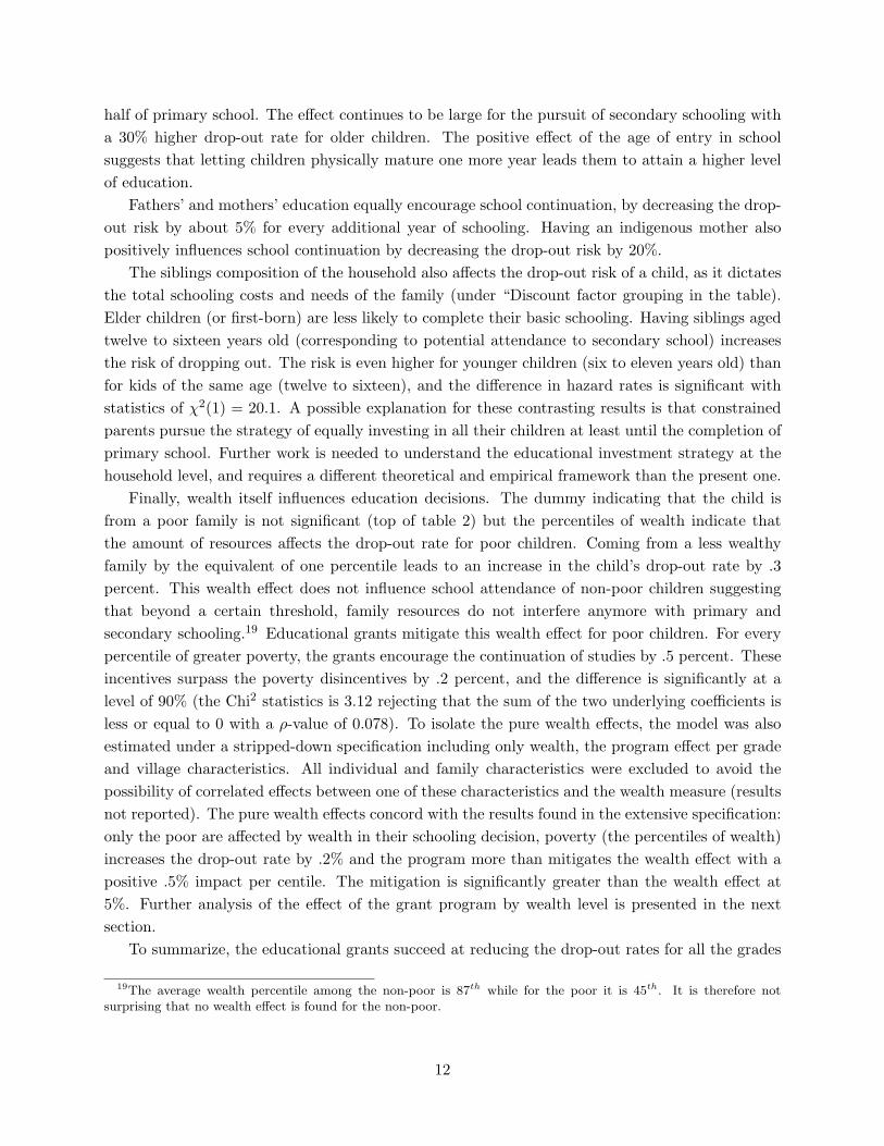
To get a better sense of how the gains vary with poverty, we repeated the procedure to estimatethe gains in schooling attainment by percentiles rather than quartiles. This allows to get a bettersense of how the .3% gain for each one percentile found in the proportional hazard estimationcumulate over the schooling career of the child to increase his total schooling attainment. Figure3 shows these gains, which due to the smaller number of observations used for each one of themexhibit greater variation than the quartile estimates. A kernel estimation22 reveals a decreasingquasi-monotonic trend in the gains as the welfare of the family increases, that is moving righttowards higher percentiles of the wealth, confirming the results found with the quartiles.

We turn next to the dimension of parents’ education. Throughout the literature, parents’education has been repeatedly shown to influence schooling (Handa 1996, Behrman and Knowles1999, Tansel 2002, for example), and the results in table 2 add further evidence. On the one hand,higher education may directly translate into higher preferences for education and thus educatedparents invest more in their children’s education. On the other hand, more educated individualshave higher earning opportunities allowing them to achieve schooling outcomes for their childrencloser to the optimal level. Hence, if the preference effect dominates, educated families will takegreater advantage of grants than less educated families. Alternatively if the financial constraintsare tighter for less educated parents, their children could benefit most from grants like Progresa.

The results tend to support the later in the case of Mexican children (table 5). Childrenfrom families where the father has no education gain twice as much from the program than theircounterparts with an educated father. This difference in gains is particularly important for boysand less so for girls. On the other hand, the mother’s education influences less the gains. Theinitial gap, seen in the control group, is smaller as children with an uneducated mother achieve asignificant .3 year (the standard error calculated by bootstrap is .07) more schooling than thosewith an uneducated father. When gains are calculated for boys and girls separately, similar resultsas under the father’s education are found (results not reported). This result comes a little as asurprise since girls receive higher grants than boys in secondary school. Yet, work by Desmombynes(2002) shows that the barriers for girls lie in the sibling composition - more particularly in havingsiblings of the same age or younger. Schooling attainment for eligible children from uneducatedfamilies remains however well below that of children from educated families - for example, 6.6 yearsof schooling for eligible children from uneducated fathers compared to 7.2 years for control childrenfrom educated fathers.

The last criterion to assess differentiated impact deals with supply constraints to education. Asresults in the previous section indicate, the distance to the closest secondary school considerably

22With a bandwidth of 0.4, i.e. using 40% of the observations of the central points The number of observationsdiminishes to 20% as you move to either end of the graph, and is 40% for the central points.

14

discourages school continuation. 31% of the children in the sample live in a village that enjoys asecondary school, while the average distance to school is 3.2 kilometers for the others, and is greaterthan 3 kilometers for 32%. Building schools in all villages is not a financially viable solution as alarge number of the villages have few children in age to attend secondary school (the sample has75% of the villages with fewer than 40 school-aged children). As indicated by Coady and Parker(2002), the demand-side approach in the form of educational transfers is more cost-effective thana program of school construction for the Mexican rural areas at large.

Educational grants effectively reduce the gap between children with and without a school intheir village (table 6). Children traveling more than three kilometers gain 0.74 year compared to0.4 for children with a school close by. With financial help and incentives, educational attainmentof children living far from school can be raised substantially from 6.3 years to 7.1 years of schooling,at a level nearing the one achieved by children with a school in their village (7.4 years in the controlgroup).

In conclusion, Progresa grants prove to differentially reach the more disadvantaged childrenalong the three dimensions analyzed. Educational grants successfully eliminate schooling attain-ment differences along the wealth dimension: independently of the wealth of their families, all thechildren receiving Progresa grants exhibit the same schooling attainment of 7.4 years. It shouldhowever be noted that even though children with uneducated parents and who live more thanthree kilometers away from a school experience among the largest gains, their schooling attainmentremain significantly lower than the average of 7.4 years for all eligible children and at times evenlower than the attainment of some control children who don’t receive grants.

6 Conclusion

Educational grants offer a demand-side intervention to address problems of low schooling attain-ment. The experience in Mexico proves that such demand-side approach can effectively counterthe effect of poverty and even further lower drop-out rates of poor children. While drop-out ratesincrease by .3% going down each percentile in poverty, the grants more than compensate this effectby reducing the drop-out rate by .5% for every percentile of poverty. These gains cumulate to raiseschooling attainment of poor children by .6 year. Most importantly, the cumulative gain amountsto leveling the playing fields for poor children - they achieve the same schooling of 7.4 years aschildren from wealthier families.

This gap closing effect is the product of the neediest children gaining the most from the program.Children of the bottom half of the wealth distribution experience gains of .8 year while the upperhalf have their schooling attainment increase by .4 year. The program did not have any built-inrule or scheme to achieve progressive gains in schooling. Hence, the equalizing result is remarkable.

The educational grants have other progressive impacts of interest. In the dimensions of parents’education and distance to school, benefits accrue particularly to children with the greatest barri-ers. Uneducated parents take advantage of the program more than their educated counterparts.However, it should be noted that while the gains are the largest, the schooling attainment continueto lag behind the average by .6 year.

15

Similarly, children that have to travel the most to get to school benefit the most from theprogram, although their schooling still falls short that of children with a school in their village by.3 year. The grants thus offer an additional policy option to supply-based approaches to raisingschooling attainment in areas not too remote from schools. Yet, they do not guarantee a silverbullet to resolve accessibility issues.

Much further analysis will be needed to determine when and to what extent educational grantscan effectively counter the effect of poverty onto schooling outcomes. Opportunities to extendthe understanding of educational grants effectiveness and impact are growing as other countrieshave initiated similar programs and the Mexican government has extended Progresa to urbanareas. Many questions could not be answered here: what is the optimal grant level? What isthe optimal grant level that insure the progressive impacts? Can grants completely close thegap in schooling between children of educated and uneducated parents? How can a demand-side approach be combined with a supply-side approach to eliminate the accessibility issues? TheMexican program Progresa has proved that poor children can achieve schooling levels comparable tothose of wealthier children. Answering the above questions shall determine how to design programsto further improve school attainment.

16

References

Akabayashi, H. and G. Psacharopoulos, “The Trade-off between Child Labour and HumanCapital Formation: A Tanzanian Case Study,” Journal of Development Studies, 1999, 35 (5),120–140.

Akhtar, S., “Do Girls Have a Higher School Drop-out Rate than Boys? A Hazard Rate Analysisof Evidence from a Third World City,” Urban Studies, 1996, 33 (1), 49–62.

Alderman, H., P. F. Orazem, and E. M. Paterno, “School Quality, School Cost and thePublic-Private School Choices of Low-Income Households in Pakistan,” Journal of HumanResources, 2001, 36 (2), 304–326.

Angrist, J. D., E. Bettinger, E. Bloom, E. King, and M. Kremer, “Vouchers for Pri-vate Schooling in Colombia: Evidence from a Randomized Natural Experiment,” AmericanEconomic Review, December 2002, 92 (5), 1535–1558.

Behrman, J., P. Sengupta, and P. Todd, “Progressing Through Progresa: An Impact Assess-ment of a School Subsidy Experiment,” April 2001. University of Pennsylvania.

Behrman, J. R. and J. C. Knowles, “Household Income and Child Schooling in Vietnam,”The World Bank Economic Review, 1999, 13 (2), 211–256.

and P. E. Todd, “Randomness in the Experimental Samples of Progresa,” March 26, 1999.Washington, DC: Progresa Evaluation Project of IFPRI, mimeo.

Binder, M., “Family Background, Gender and Schooling in Mexico,” Journal of DevelopmentStudies, 1998, 35 (2), 54–71.

Bommier, A. and S. Lambert, “Education Demand and Age at School Enrollment in Tanzania,”Journal of Human Resources, 2000, 35 (1), 177–203.

Coady, D. P. and S. Parker, “A Cost-Effectiveness Analysis of Demand- and Supply-side Edu-cation Interventions: The Case of Progresa in Mexico,” March 2002. Food Consumption andNutrition Division Discussion Paper 127, IFPRI.

de Leon, J. G., D. Hernandez, and S. Parker, “Intergenerational Transmission of Poverty inMexico: The Impact of the Education, Health and Nutrition Program (Progresa),” June 1999.Mexico DF: National Cordination of Progresa, mimeo.

Desmombynes, G., “Sibling Composition, Gender and the Effects of School Grants in RuralMexico,” November 2002. University of California, Berkeley, mimeo.

Glewwe, P. and H. Jacoby, “Student Achievement and Schooling Choice in Low-Income Coun-tries: Evidence from Ghana,” Journal of Human Resources, 1994, 29 (3), 842–864.

Grambsch, P.M. and T.M. Therneau, “Proportional Hazards Tests and Diagnostics Based onWeighted Residuals,” Biometrika, 1994, 81, 515–526.

Handa, S., “The Determinants of Teenage Schooling in Jamaica: Rich vs. Poor, Females vs.Males,” Journal of Development Studies, 1996, 32 (4), 554–580.

17

, “Raising Primary School Enrollment in Developing Countries - the Relative Importance ofSupply and Demand,” Journal of Development Economics, 2002, 69 (1), 103–28.

Kiefer, N.M., “Economic Duration Data and Hazard Functions,” Journal of Economic Literature,June 1988, 26, 646–679.

Kim, J., H. Alderman, and P. F. Orazem, “Can Private School Subsidies Increase Enrollmentfor the Poor? The Quetta Urban Fellowship Program,” World Bank Economic Review, 1999,13 (3), 443–65.

Lavy, V., “School Supply Constraints and Children’s Educational Outcomes in Rural Ghana,”Journal of Development Economics, 1996, 51, 291–314.

Lillard, L.A. and R.J. Willis, “Intergenerational Educational Mobility: Effects of Family andState in Malaysia,” Journal of Human Resources, 1994, 29 (4), 1126–1166.

Lopez-Acevedo, G., “Learning Outcomes and School Cost-Effectiveness in Mexico: The PareProgram,” Working Paper 2128, World Bank May 1999.

Muniz, P.E., “La Situacion Escolar en Localidades Rurales Marginadas en Mexico,” 1999. MexicoDF: National Cordination of Progresa, mimeo.

Schultz, T. P., “School Subsidies for the Poor: Evaluating the Mexican Progresa Poverty Pro-gram,” 2001. forhcoming in Journal of Development Economics.

Skoufias, E. and S. Parker, “Conditional Cash transfers and their Impact on Child Work andSchooling: Evidence from the Progresa Program in Mexico,” October 2001. Food Consumptionand Nutrition Division Discussion Paper 123, IFPRI.

Tansel, A., “Schooing Attainment, Parental Education, and Gender in Cote d’Ivoire and Ghana,”Economic Development and Cultural Change, 1997, 45 (4), 825–856.

, “Determinants of School Attainment of Boys and Girls in Turkey: Individual, householdsand Community Factors,” Economics of Education Review, 2002, 21 (5), 455–70.

West, E.G., “Education Vouchers in Principle and Practice: A Survey,” World Bank ResearchObserver, February 1997, 12 (1), 83–103.

18

Co

ntin

ua

tio

n r

ate

(%

)

Grade1p 2p 3p 4p 5p 6p 1s 2s 3s

.6

.65

.7

.75

.8

.85

.9

.95

1

Figure 1: Continuation rate for grades of primary and secondary school (Progresa data).

Ra

tio

of

gra

de

ba

se

line

ha

za

rd t

o a

ve

rag

e o

fp

rim

ary

gra

de

s b

ase

line

ha

za

rds

Grade to enter1p 2p 3p 4p 5p 6p 1s 2s 3s

0

4

8

12

16

20

2.7

1.51.1

.3 .2 .2

18.1

2.12.5

Figure 2: Non-parametric estimates of the baseline hazard rate.

19

Ga

ins in

sch

oo

ling

att

ain

me

nt

(in

ye

ars

)

Percentile of wealth index

Calculated gain Kernel estimation

0 25 50 75 100

−1

−.5

0

.5

1

1.5

2

Figure 3: Kernel estimation of the gain in school attainment by poverty level.

Table 1: Progresa educational monthly grants by grade and gender.

Grant (in pesos)Grade July 1998 July 1999 Jan 2000

primary3 70 80 854 80 95 1005 100 125 1306 135 165 170

secondary boy girl boy girl boy girl1 200 210 240 250 250 2652 210 235 250 280 265 2953 220 255 265 305 280 320

Maximum per family 625 750 7909 pesos is worth about US$1.

Grants are adjusted every six months for inflation.

Source: National Direction of Progresa, 2000

20

Table 2: Impact of Progresa on the conditional probability to drop out of school.

Hazard Ratio Z stata

Year 1998 dummy 1.00 -0.05Progresa village (α1) 0.99 -0.14Eligible family (α2) 1.56 1.46

Costs (Cg+1)Distance to school1 (in km) 1.20 8.69 ∗∗∗

Distance over 3 km 0.82 -5.79 ∗∗∗

Earnings (w(g, Z))Off-farm earning opportunities

Share of employment sectors in the village2,5

Agricultural sector (0-100) 1.01 4.33 ∗∗∗

Non-agricultural sector (0-100) 1.03 7.10 ∗∗∗

Other employment types (0-100)6 1.02 4.15 ∗∗∗

Village average level of schooling (0-6 yrs) 0.78 -6.88 ∗∗∗

Distance to capital (per 10 Km)2 0.98 -5.88 ∗∗∗

Family’s labour needsFamily owes business3 1.06 1.01Agricultural land cultivated by the family (in Ha)

for a child aged 8-11 0.92 -2.21 ∗∗

for a child aged 12-16 1.00 0.32# of draft animals2 1.01 1.84 ∗

# of cattle heads 0.99 -1.33# of small productive animals 1.00 -0.05# of 0-5 yr old children3 1.05 2.34 ∗∗

Child’s work opportunitiesAge dummy for 8 years and older 1.15 0.43Age dummy for 12-16 years old 1.24 0.72Work while in school the year before 1.00 -0.03Girl in primary school 0.92 -0.93Girl in secondary school 1.17 3.94 ∗∗∗

Child’s ability (Z)Entry age to primary school 0.93 -2.44 ∗∗

Child failed his grade the previous yearGrade 1-3 1.25 1.25Grade 4-6 2.05 7.11 ∗∗∗

Grade 7-9 1.69 10.51 ∗∗∗

Age (proxy for school progression)In grade 1-3 1.62 13.00 ∗∗∗

In grade 4-6 1.73 17.14 ∗∗∗

In grade 7-9 1.30 14.74 ∗∗∗

continued on next page

21

continued from previous page

Hazard Ratio Z stata

Parents’ human capital (Z)Mother’s schooling (in years) 0.96 -4.06 ∗∗∗

Father’s schooling (in years) 0.94 -5.96 ∗∗∗

Indigenous mother 0.79 -2.04 ∗∗

Indigenous father 0.88 -1.14Discount factor (β)Birth order4

In primary school 0.56 -7.26 ∗∗∗

In high school 0.81 -4.55 ∗∗∗

# of siblings aged 6 to 11for a child aged 6-11 0.98 -0.17for a child aged 12-16 1.00 0.00

# of siblings aged 12 to 16for a child aged 6-11 1.61 5.78 ∗∗∗

for a child aged 12-16 1.10 3.72 ∗∗∗

Wealth (δ)Percentile of wealth index for non-poor 1.002 0.65Percentile of wealth index for poor 0.997 -2.07 ∗∗

Treatment effects (Tg+1)By grade (γh)

Primary 3 0.48 -2.81 ∗∗∗

Primary 4 0.46 -3.49 ∗∗∗

Primary 5 0.61 -2.33 ∗∗

Primary 6 0.54 -3.60 ∗∗∗

Secondary 1 0.55 -4.86 ∗∗∗

Secondary 2 0.57 -2.70 ∗∗∗

Secondary 3 0.52 -3.17 ∗∗∗

By percentile of wealth (ζ) 1.005 2.91 ∗∗∗

No. of observations = 35387No. of subjects = 20541Overall Chi2 = 3507Log Likelihood = -17483Time Varying Hazard test, Chi2 = 43a Z statistics associated with the underlying coefficient. A Huber correction is used to obtain robust error

estimates at the family level.∗ significant at 90% ∗∗ significant at 95% ∗∗∗ significant at 99%1 For high school grades only; 2 For teens 12-16 years old only; 3 For children 8 years and older; 4 1 =

Eldest, 2 = Second child, ...; 5 Against the share of self-employed individuals; 6 Includes non-renumerated

work, work for a cooperative and work in a communal farm (ejido).

22

Table 3: Predicted schooling attainment and gains from Progresa grants.

Schooling Attainment Gain(in years) over control

Non-Poor1 7.3(.07)

Poor in control villages 6.8(.07)

Poor in treatment villages1. Current program covering 7.4 0.56 ∗∗

primary 3 to secondary 3 (.05) (.07)2. Program in secondary 1 only 7.0 0.22 ∗∗

(.10) (.11)

Difference in gains 0.34 ∗∗

(Treatment 1. vs 2.) (.09)Note: The standard errors calculated by bootstrapping the complete estimation procedure

are found in parenthesis.∗∗ indicates significant at 95% and ∗ significant at 90%.1 Includes the non-poor from Progresa and non-Progresa villages.

Table 4: Predicted schooling attainment E[G] and gains by wealth among eligible households.

E[G] (in years) GainTreatment Control over control

Wealth index, by quartileFirst 7.3 6.4 0.88 ∗∗

(.08) (.11) (.13)Second 7.4 6.6 0.86 ∗∗

(.06) (.10) (.10)Third 7.4 7.0 0.37 ∗∗

(.07) (.08) (.10)Fourth 7.3 7.0 0.35 ∗∗

(.10) (.10) (.13)

Diff in gains First vs second 0.02(.14)

Second vs third 0.49 ∗∗

(.12)Note: The standard errors calculated by bootstrapping the complete estimation procedure

are found in parenthesis.∗∗ indicates significant at 95% and ∗ significant at 90%.

23

Table 5: Predicted schooling attainment E[G] and gains by parents’ education.

E[G] (in years) Gain DiffTreatment Control over control in gains1

Father’s educationNone 6.6 5.7 0.86 ∗∗

(.09) (.13) (.13) 0.40 ∗∗

Some 7.6 7.2 0.46 ∗∗ (.11)(average = 4.2) (.05) (.06) (.07)

For girlsNone 6.6 5.8 0.73 ∗∗

(.10) (.17) (.16) 0.25 ∗

Some 7.6 7.2 0.48 ∗∗ (.15)(.06) (.07) (.08)

For BoysNone 6.5 5.6 0.97 ∗∗

(.13) (.16) (.18) 0.53 ∗∗

Some 7.6 7.2 0.44 ∗∗ (.17)(.06) (.07) (.07)

Mother’s educationNone 6.7 6.0 0.65 ∗∗

(.10) (.11) (.12) 0.15Some 7.7 7.2 0.50 ∗∗ (.10)(average = 4.2) (.04) (.06) (.07)

Note: The standard errors calculated by bootstrapping the complete estimation procedure are found

in parenthesis.∗∗ indicates significant at 95% and ∗ significant at 90%.1 Tests Gain(None) - Gain(Some)=0.

24

Table 6: Predicted schooling attainment E[G] and gains by distance to school.

E[G] (in years) GainTreatment Control over control

Distance to high schoolWithin 1 Km 7.8 7.4 0.40 ∗∗

(.06) (.07) (.07)Between 1 to 3 Km 7.4 6.7 0.64 ∗∗

(.06) (.08) (.08)Beyond 3 Km 7.1 6.3 0.74 ∗∗

(.06) (.09) (.09)

Diff in gains 1 Km vs 1-3 Km 0.24 ∗∗

(.06)1-3 Km vs 3 + Km 0.10

(.08)1 Km vs 3 + Km 0.34 ∗∗

(.08)Note: The standard errors calculated by bootstrapping the complete estimation procedure

are found in parenthesis.∗∗ indicates significant at 95% and ∗ significant at 90%.

25