Edmund Cannon

Banking CrisisUniversity of Verona

Lecture 2

Plan for today2

Brief review of yesterday

Opportunity for questions

Leverage in the banking system

Effect of limited liability

Systemic risk

Remember yesterday!3

Banks are financial institutions that engage in “maturity transformation”:

Banks borrow short-term (a breve termine)

Banks lend long-term (a lungo termine)

Diamond-Dybvig model – banks are unstable (two Nash equilibria).

Potential solutions:

Central bank intervention (Bagehot)

Deposit insurance

What else is important about banks?4

Banks engage in maturity transformation.

Another important feature of banks:

Banks are leveraged.

Nb other institutions are leveraged too:

Leveraged Not leveraged

General assurance (insurance) companyLife assurance companyHedge fundSupermarket

Mutual fundRatings agencyStock brokerAccountantActuary

A very simple model of a bank’s balance sheet5

Assets Liabilities

Loans €90 Equity €8

Cash €10 Deposits

€92

Total €100

Total €100

(Simple definition):

AssetsLeverage

Equity=

A More Detailed Model of a Bank Balance Sheet

6

Difference between equity and depositors/bondholders.

7

Depositors and bond-holders (should) have no risk.

They should not get back less than they deposit plus interest (no downside risk);

They will not get back more than they deposit plus interest (no upside risk).

Equity holders (sometimes referred to as capital):

Should bear all of the risk (upside and downside risk);

They get the residual (= profit).

Contrast this model with basic money supply model of banking (implications for macroeconomic models such as IS-LM)

8

{ { { Total Money OutsideMoney Supply Multiplier Money

Money supply constrained by

M m H£ ´

{ { {

{ { {

Total Money OutsideMoney Supply Multiplier Money

Equity Supply Leverageof Credit Ratio

Money supply and credit constrained by

M m H

M El*

£ ´

£ ´

A mutual fund (“unit trust” in the UK)9

AssetsLeverage i.e. not levered.

Equity1,= =

Selling short on equity (eg hedge fund)

10

Equity "risky assets"Leverage

Equity

nb "risky assets"

-

0

=

<

Losses and leverage11

Suppose a firm is levered by a factor of ten.

The firm can bear losses of up to 10% (=1/10) before equity is exhausted.

If leverage is twenty then the firm can only bear losses of 5%.

Leverage in 2007:

Goldman Sachs 25

Lehman Bros 29

Merrill Lynch 32

Trends in leverage in USA and UKSource: Turner Report12

Is Leverage a “Good” or “Bad” Thing?13

Greater leverage allows more investment.

Leverage allows risk to be shared in a particular way (equity bears more risk, bonds bear less risk)

If assets are over-priced then short-selling helps correct the price – but short selling typically involves leverage.

Too much leverage means that bond-holders are exposed to risk (which they are trying to avoid).

Leverage results in limited liability for the equity holders: downside risk is borne by bond holders (or government).

Leverage endogenises risk (Shin, 2009)

Risk aversion: concave preferences14

2

20 0

U U

C C

Limited liability and risk aversion: U = ln(W)15

In the bad state of the world the payoff to the risky

investment is 1.1 – e.

This might be less than one (negative return). But

our utility function is not defined for negative utility

(perhaps because consumption cannot be negative).

Risk aversion with limited liability16

Limited liability and risk aversion: U = ln(W)17

0.09

0.10

0.10

0.11

0.11

0.12

0.12

0.13

0.13

0.14

0.00

0.02

0.04

0.06

0.08

0.10

0.12

0.14

0.16

0.18

0.20

Expected utility

Value of e

Limited liability and risk aversion18

Even risk-averse agents may like riskier investments

if they have limited liability.

Banking: excessive risk means bad outcomes fall on

bondholders, depositors and the government (via

insurance).

Limited liability may be one of the causes of

the financial crisis (faulty incentives or

bankers).

BUT:

Perhaps bankers are risk-neutral or risk-loving;

Perhaps bankers are irrational.

Reducing risks in banks19

Banks might be required or choose to self-insure.

Ownership structure (partnerships) and

competition.

Separate retail and investment banking:USA: Glass-Steagall Act (1933), repealed 1999USA: Frank-Dodd Act (2010)UK: Vickers Commission proposal (2010)

Capital requirements (Basel I, etc)

Supervision or RegulationModelling / measuring risk (Basel II, second tier)Making information publicly available (Basel II, third tier)

Capital Requirements: Basel I, II, III20

Basel I: International agreement of 1988: implemented in 1990s.

Capital requirement of 8% so leverage of 12½.

Leverage is defined as ratio of capital (equity) to risk-weighted assets.

The risk weights depend upon credit ratings, determined by credit rating agencies.

Basel II and III changed the weights and ratios. USA introduced the “recourse rule” rather than Basel II (very similar).

Basel I and Basel II capital requirements

21Risk-weighted Assets

Leverage ( capital)Total Capital

12

12 8%= <

Basel I Basel II

Weight Capital Weight Capital

Cash 0% none 0% none

Gov’t Bonds

AAA/AA 0% none 0% none

A 0% none 20% 1.6%

BBB 0% none 50% 4.0%

BB/B 0% none 100% 8.0%

Agency bonds 20% 1.6% 20% 1.6%

Asset-backed securities

AAA/AA 100% 8.0% 20% 1.6%

A 100% 8.0% 50% 4.0%

BBB/BB 100% 8.0% 100% 8.0%

Mortgages 50% 4.0% 35% 2.4%

Business loans 100% 8.0% varies

Three sorts of capital requirement22

Basel II Basel III Basel III +

counter-cyclical buffer

UK’sVickers

Commission

Tier 1 Equity / Risk-Weighted Assets

2% 3½ % 6% 7%

10%

Total Capital / Risk-Weighted Assets

8% 8% 10½ %

Tier 1 Equity / Total Assets

3%

Credit Ratings23

e.g. Moody’s

Grade

Expected 10-year loss

Comment

Aaa 0.01% Highest grade

Investment Grade

Aa 0.06% - 0.22% Very low risk

A 0.39% - 0.99% Low risk

Baa 1.43% - 3.36% Moderate risk

Ba 5.17% - 9.71% Questionable quality

Speculative Grade(Junk bonds)

B 12.21% - 19.12% Poor quality

Caa 35.75% Extremely poor

Ca, C Possibly in default

Problems with the credit rating industry24

Ratings agencies have quasi-official status

ie when a bank justifies the risk on its balance sheet to a regulator it uses a recognised agency’s ratings.

Very few firms (Moody’s, Fitch, Standard & Poors)

Reputation

Needs to be officially recognised.

Too much reliance on ratings agencies.

Agencies are paid by the issuer of an asset (ie the borrower) not the purchaser of the asset (the lender). This creates an incentive problem.

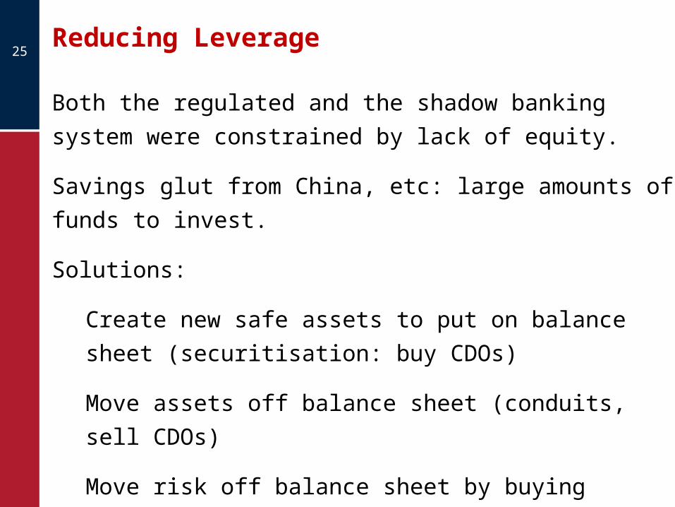
Reducing Leverage25

Both the regulated and the shadow banking system

were constrained by lack of equity.

Savings glut from China, etc: large amounts of funds

to invest.

Solutions:

Create new safe assets to put on balance sheet

(securitisation: buy CDOs)

Move assets off balance sheet (conduits, sell CDOs)

Move risk off balance sheet by buying insurance

(Credit Default Swaps)

Securitisation: Mortgages26

US market is very different to Europe (where little securitisation)

Prime mortgagesSold with strict underwiting standards;Passed on to Fannie Mae / Freddie Mac (state sponsored);Then sold as agency RMBSs.

Sub-prime mortgagesSold with weaker underwriting;Bundled together into securities by investment banks.Sold on as RMBSs.Difficult to work out quality of underlying mortgages.

Creating “safe” assets: Collateralised Debt Obligations (CDOs)

27

Collateralised debt obligations are similar to SIVs

except

they lend long and borrow long (no maturity

transformation);

they are not open ended.

Tett describes how these were pioneered by

JPMorgan.

When based on mortgages referred to as

Collateralised Mortgage Obligations (CMOs) or

Residential Mortgage-Backed Securities (RMBSs).

Reasons for creating Collateralised Debt Obligations (CDOs)

28

(i) (Simple situation) The bank acts as an

intermediary but neither the asset nor the

liability appear on the balance sheet.

Therefore, this avoids capital requirements.

(ii) The bank can create new financial assets with

differing levels of risk (securitisation;

tranching)

Simple Model29

In this model there are two borrowers, X and Y.

Each borrower will either

Repay a loan of £100 (probability of 0.9)

Default and repay nothing (probability of 0.1)

(This model is not very realistic, but the maths is simple.)

We start by assuming that whether or not X repays is independent of whether or not Y repays.

Simple Model (continued)30

So there are three possibilities:

Both borrowers repay (probability 0.81)

Just one borrower repays (probability 0.18 = 0.09 + 0.09)

Both borrowers default (probability 0.01)

No correlation

Borrower X

Borrower Y

Default prob = 0.1

Repay prob = 0.9

Default prob = 0.1 0.01 0.09

Repay prob = 0.9 0.09 0.81

31

2 2

E Loan X to A 0.9 100 0.1 0 90

var Loan X to A 0.9 100 90 0.1 0 90 900

st.dev. Loan X to A 900 30

Loan Y has the same characteristics as Loan

X.

Saving and borrowing without risk pooling (no FI)

32

Each saver gets half of the money paid into the

mutual fund.

Saving and borrowing with risk pooling (mutual fund)

33

( ) ( )

( )

E Either X or Y

var Either X or Y

st.dev. Either X or Y

2 2

2

0.81 200 0.18 100 0.01 090

2

0.81 100 90 0.18 50 0

0.01 0 90

450

450 21

´ + ´ + ´é ù= =ê úë û

é ù= ´ - + ´ -ê úë û

+ ´ -

=

é ù= »ê úë û

34

So long as there is money available, the senior

tranche gets paid (i.e., senior tranche gets paid

first).

The junior tranche only gets paid after the senior

tranche

Saving and borrowing with tranching (securitisation)

35

( ) ( )

E Senior tranche

var Senior tranche

st.dev. Senior tranche

2 2

0.99 100 0.01 0 99

0.99 100 99 0.01 99 0 99

10

é ù= ´ + ´ =ê úë û

é ù= ´ - + ´ - =ê úë ûé ù»ê úë û

X and Y repay: repaidSenior tranche receives

only one repays: repaid

neither repays: repaid Senior tranche receives zero

200 0.81100

100 0.18

0 0.01

p

p

p

üï= ïïýï= ïïþ

=

36

( ) ( )

E Junior tranche

var Junior tranche

st.dev. Junior tranche

2 2

0.81 100 0.19 0 81

0.81 100 81 0.19 81 0 1539

1539 39

é ù= ´ + ´ =ê úë û

é ù= ´ - + ´ - =ê úë û

é ù= »ê úë û

X and Y repay: repaid Junior tranche receives

only one repays: repaidJunior tranche receives zero

neither repays: repaid

200 0.81 100

100 0.18

0 0.01

p

p

p

=

üï= ïïýï= ïïþ

Discussion of Model37

By pooling risky assets it is possible to reduce overall risk.

The underlying mortgage had a st.dev. of 30

A mutual fund of two mortgages had a st.dev. of 21

The senior tranche of a securitised CMO had a st.dev. of 10.

In the example the risky assets were uncorrelated. It is still possible to reduce risk in a mutual fund (equal sharing of assets) even if assets are positively correlated (so long as they are not perfectly correlated). The effect of correlation on the value of tranches is more complicated.

Risk pooling with differing degrees of correlation38

No correlation0.1 0.9

0.1 0.01 0.090.9 0.09 0.81

Variance 450

Partial correlation in payoff

0.1 0.90.1 0.05 0.050.9 0.05 0.85

Variance 650

Perfect correlation in payoff

0.1 0.90.1 0.1 00.9 0 0.9

Variance 900

Negative correlation in payoff

0.1 0.90.1 0 0.10.9 0.1 0.8

Variance 400

Securitisation39

Pool a group of risky assets into a Special

Purpose Vehicle.

The payouts of the SPV are then tranched:

Tranche 1 (Super-senior) gets first call on

assets

Tranche 2 (Senior) goes next

Tranche 3 (Mezzanine) goes next

Tranche 4 (Junk) gets anything left.

Possible to create AAA-rated assets from

underlying assets with a much lower credit

rating.

US: Special Purpose Entity; Eire: Financial Vehicle Corporation

Securitisation: Mortgages40

US market is very different to UK (where little

securitisation)

Prime mortgages

Sold with strict underwiting standards;

Passed on to Fannie Mae / Freddie Mac (state

sponsored);

Then sold as RMBSs.

Sub-prime mortgages

Sold with weaker underwriting;

Bundled together into securities by investment

banks.

Sold on as RMBSs.

Difficult to work out quality of underlying

mortgages.

Pricing of any RMBS depends upon the

correlation.

Insurance41

Credit Default Swaps: part (i)42

Credit Default Swaps: part (ii)43

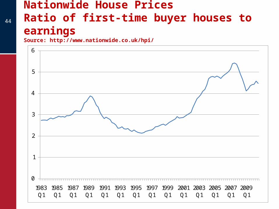
Nationwide House PricesRatio of first-time buyer houses to earningsSource: http://www.nationwide.co.uk/hpi/

44

0

1

2

3

4

5

6

1983 Q1

1985 Q1

1987 Q1

1989 Q1

1991 Q1

1993 Q1

1995 Q1

1997 Q1

1999 Q1

2001 Q1

2003 Q1

2005 Q1

2007 Q1

2009 Q1

Ratio of house prices to average earningsSource: Nationwide, National Statistics, author’s calculations

45

0

1

2

3

4

5

6

1963

1965

1967

1969

1971

1973

1975

1977

1979

1981

1983

1985

1987

1989

1991

1993

1995

1997

1999

2001

2003

2005

2007

2009

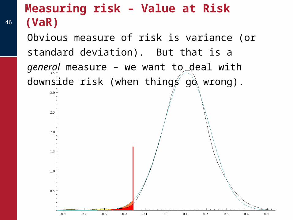
Measuring risk – Value at Risk (VaR)46

Obvious measure of risk is variance (or

standard deviation). But that is a general

measure – we want to deal with downside risk

(when things go wrong).

Difficulty of estimating VaR from data

47

Distribution of VaR Measure - quantile Distribution of VaR Measure - t(10) N(s=0.114)

Distribution of VaR Measure - Normal approx Distribution of Returns ~ t(10)

-0.5 -0.4 -0.3 -0.2 -0.1 0.0 0.1 0.2 0.3 0.4 0.5

5

10

15

20

25

30

35Distribution of VaR Measure - quantile Distribution of VaR Measure - t(10) N(s=0.114)

Distribution of VaR Measure - Normal approx Distribution of Returns ~ t(10)

Leverage and endogenous risk (Shin)48

Endogenous risk – the crash49

As asset prices fall (losses mount) leverage rises.

Firms sell assets to reduce leverage.

Firesale prices are an externality to other banks’

balance sheets (especially with mark-to-market

pricing).