Edge Detection iOS Apps

www.letsnurture.com

www.letsnurture.com

Edge detection is the name for a set of mathematical methods which aim at identifying points in a digital image at which the image brightness changes sharply or, more formally, has discontinuities.

The points at which image brightness changes sharply are typically organized into a set of curved line segments termed edges.

The same problem of finding discontinuities in 1D signals is known as step detection and the problem of finding signal discontinuities over time is known as change detection.

Edge detection is a fundamental tool in image processing, machine vision and computer vision, particularly in the areas of feature detection and feature extraction

www.letsnurture.com

Development of the Canny algorithm

Edge detection, especially step edge detection has been widely applied in various different computer vision systems, which is an important technique to extract useful structural information from different vision objects and dramatically reduce the amount of data to be processed.

Canny has found that, the requirements for the application of edge detection on diverse vision systems are relatively the same.

Thus, a development of an edge detection solution to address these requirements can be implemented in a wide range of situations.

www.letsnurture.com

The general criteria for edge detection includes

Detection of edge with low error rate, which means that the detection should accurately catch as many edges shown in the image as possible

The edge point detected from the operator should accurately localize on the center of the edge.

A given edge in the image should only be marked once, and where possible, image noise should not create false edges.

www.letsnurture.com

To satisfy these requirements Canny used the calculus of variations – a technique which finds the function which optimizes a given functional.

The optimal function in Canny's detector is described by the sum of four exponential terms, but it can be approximated by the first derivative of a Gaussian.

Process of Canny edge detection algorithm

The Process of Canny edge detection algorithm can be broken down to 5 different steps:

•Apply Gaussian filter to smooth the image in order to remove the noise•Find the intensity gradients of the image•Apply non-maximum suppression to get rid of spurious response to edge detection•Apply double threshold to determine potential edges•Track edge by hysteresis: Finalize the detection of edges by suppressing all the other edges that are weak and not connected to strong edges.

www.letsnurture.com

Use the OpenCV function Canny to implement the Canny Edge Detector.

TheoryThe Canny Edge detector was developed by John F. Canny in 1986.

Also known to many as the optimal detector, Canny algorithm aims to satisfy three main criteria:

Low error rate: Meaning a good detection of only existent edges.

Good localization: The distance between edge pixels detected and real edge pixels have to be minimized.

Minimal response: Only one detector response per edge.

www.letsnurture.com

1.Filter out any noise. The Gaussian filter is used for this purpose. An example of a Gaussian kernel of that might be used is shown below:

www.letsnurture.com

Find the intensity gradient of the image. For this, we follow a procedure analogous to Sobel:

Apply a pair of convolution masks (in x and y directions:

www.letsnurture.com

Find the gradient strength and direction with:

The direction is rounded to one of four possible angles (namely 0, 45, 90 or 135)

www.letsnurture.com

Non-maximum suppression is applied.

This removes pixels that are not considered to be part of an edge. Hence, only thin lines (candidate edges) will remain.

Hysteresis: The final step. Canny does use two thresholds (upper and lower):

If a pixel gradient is higher than the upper threshold, the pixel is accepted as an edge

If a pixel gradient value is below the lower threshold, then it is rejected.

If the pixel gradient is between the two thresholds, then it will be accepted only if it is connected to a pixel that is above the upper threshold.

Canny recommended a upper:lower ratio between 2:1 and 3:1.

www.letsnurture.com

What does this program do?

Asks the user to enter a numerical value to set the lower threshold for our Canny Edge Detector (by means of a Trackbar)

Applies the Canny Detector and generates a mask (bright lines representing the edges on a black background).

Applies the mask obtained on the original image and display it in a window.

www.letsnurture.com

#include "opencv2/imgproc/imgproc.hpp"#include "opencv2/highgui/highgui.hpp"#include <stdlib.h>#include <stdio.h>

using namespace cv;

/// Global variables

Mat src, src_gray;Mat dst, detected_edges;

int edgeThresh = 1;int lowThreshold;int const max_lowThreshold = 100;int ratio = 3;int kernel_size = 3;char* window_name = "Edge Map";

www.letsnurture.com

/** * @function CannyThreshold * @brief Trackbar callback - Canny thresholds input with a ratio 1:3 */void CannyThreshold(int, void*){ /// Reduce noise with a kernel 3x3 blur( src_gray, detected_edges, Size(3,3) );

/// Canny detector Canny( detected_edges, detected_edges, lowThreshold, lowThreshold*ratio, kernel_size );

/// Using Canny's output as a mask, we display our result dst = Scalar::all(0);

src.copyTo( dst, detected_edges); imshow( window_name, dst ); }

www.letsnurture.com

/** @function main */int main( int argc, char** argv ){ /// Load an image src = imread( argv[1] );

if( !src.data ) { return -1; } /// Create a matrix of the same type and size as src (for dst) dst.create( src.size(), src.type() ); /// Convert the image to grayscale cvtColor( src, src_gray, CV_BGR2GRAY ); /// Create a window namedWindow( window_name, CV_WINDOW_AUTOSIZE ); /// Create a Trackbar for user to enter threshold createTrackbar( "Min Threshold:", window_name, &lowThreshold, max_lowThreshold, CannyThreshold ); /// Show the image CannyThreshold(0, 0); /// Wait until user exit program by pressing a key waitKey(0); return 0; }

www.letsnurture.com

Create some needed variables:

Mat src, src_gray; Mat dst, detected_edges;

int edgeThresh = 1; int lowThreshold; int const max_lowThreshold = 100; int ratio = 3; int kernel_size = 3; char* window_name = "Edge Map";

Note the following:

a. We establish a ratio of lower:upper threshold of 3:1 (with the variable *ratio*)b. We set the kernel size of :math:`3` (for the Sobel operations to be performed internally by the Canny function)c. We set a maximum value for the lower Threshold of :math:’100`

www.letsnurture.com

Loads the source image:

/// Load an imagesrc = imread( argv[1] );

if( !src.data ) { return -1; }Create a matrix of the same type and size of src (to be dst)

dst.create( src.size(), src.type() );Convert the image to grayscale (using the function cvtColor:

cvtColor( src, src_gray, CV_BGR2GRAY );

www.letsnurture.com

Create a window to display the results

namedWindow( window_name, CV_WINDOW_AUTOSIZE );

Create a Trackbar for the user to enter the lower threshold for our Canny detector:

createTrackbar( "Min Threshold:", window_name, &lowThreshold, max_lowThreshold, cannyThreshold);

www.letsnurture.com

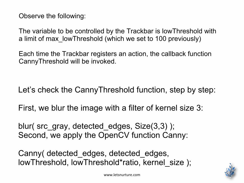
Observe the following:

The variable to be controlled by the Trackbar is lowThreshold with a limit of max_lowThreshold (which we set to 100 previously)

Each time the Trackbar registers an action, the callback function CannyThreshold will be invoked.

Let’s check the CannyThreshold function, step by step:

First, we blur the image with a filter of kernel size 3:

blur( src_gray, detected_edges, Size(3,3) );Second, we apply the OpenCV function Canny:

Canny( detected_edges, detected_edges, lowThreshold, lowThreshold*ratio, kernel_size );

www.letsnurture.com

where the arguments are:

detected_edges: Source image, grayscale

detected_edges: Output of the detector (can be the same as the input)

lowThreshold: The value entered by the user moving the Trackbar

highThreshold: Set in the program as three times the lower threshold (following Canny’s recommendation)

kernel_size: We defined it to be 3 (the size of the Sobel kernel to be used internally)

www.letsnurture.com

We fill a dst image with zeros (meaning the image is completely black).

dst = Scalar::all(0);

Finally, we will use the function copyTo to map only the areas of the image that are identified as edges (on a black background).

src.copyTo( dst, detected_edges);

copyTo copy the src image onto dst.

However, it will only copy the pixels in the locations where they have non-zero values. Since the output of the Canny detector is the edge contours on a black background, the resulting dst will be black in all the area but the detected edges.

We display our result:

imshow( window_name, dst );

www.letsnurture.com

Notice how the image is superposed to the black background on the edge regions.

www.letsnurture.com

There are two other methods of detecting edges in the image

SobelScharr

www.letsnurture.com

You can easily notice that in an edge, the pixel intensity changes in a notorious way. A good way to express changes is by using derivatives.

A high change in gradient indicates a major change in the image.

www.letsnurture.com

To be more graphical, let’s assume we have a 1D-image. An edge is shown by the “jump” in intensity in the plot below:

The edge “jump” can be seen more easily if we take the first derivative (actually, here appears as a maximum)

www.letsnurture.com

So, from the explanation in previous slide, we can deduce that a method to detect edges in an image can be performed by locating pixel locations where the gradient is higher than its neighbors (or to generalize, higher than a threshold)

Sobel Operator

The Sobel Operator is a discrete differentiation operator. It computes an approximation of the gradient of an image intensity function.

The Sobel Operator combines Gaussian smoothing and differentiation.

www.letsnurture.com

Horizontal changes: This is computed by convolving I with a kernel G_{x} with odd size. For example for a kernel size of 3, G_{x} would be computed as:

Vertical changes: This is computed by convolving I with a kernel G_{y} with odd size. For example for a kernel size of 3, G_{y} would be computed as:

At each point of the image we calculate an approximation of the gradient in that point by combining both results above:

Although sometimes the following simpler equation is used:

www.letsnurture.com

#include "opencv2/imgproc/imgproc.hpp"#include "opencv2/highgui/highgui.hpp"#include <stdlib.h>#include <stdio.h>

using namespace cv;

/** @function main */int main( int argc, char** argv ){

Mat src, src_gray; Mat grad; char* window_name = "Sobel Demo - Simple Edge Detector"; int scale = 1; int delta = 0; int ddepth = CV_16S;

int c;

/// Load an image src = imread( argv[1] );

if( !src.data ) { return -1; }

www.letsnurture.com

GaussianBlur( src, src, Size(3,3), 0, 0, BORDER_DEFAULT );

/// Convert it to gray cvtColor( src, src_gray, CV_RGB2GRAY );

/// Create window namedWindow( window_name, CV_WINDOW_AUTOSIZE );

/// Generate grad_x and grad_y Mat grad_x, grad_y; Mat abs_grad_x, abs_grad_y;

/// Gradient X //Scharr( src_gray, grad_x, ddepth, 1, 0, scale, delta, BORDER_DEFAULT ); Sobel( src_gray, grad_x, ddepth, 1, 0, 3, scale, delta, BORDER_DEFAULT ); convertScaleAbs( grad_x, abs_grad_x );

/// Gradient Y //Scharr( src_gray, grad_y, ddepth, 0, 1, scale, delta, BORDER_DEFAULT ); Sobel( src_gray, grad_y, ddepth, 0, 1, 3, scale, delta, BORDER_DEFAULT ); convertScaleAbs( grad_y, abs_grad_y );

www.letsnurture.com

/// Total Gradient (approximate) addWeighted( abs_grad_x, 0.5, abs_grad_y, 0.5, 0, grad );

imshow( window_name, grad );

waitKey(0);

return 0; }

www.letsnurture.com

First we declare the variables we are going to use:

Mat src, src_gray;Mat grad;char* window_name = "Sobel Demo - Simple Edge Detector";int scale = 1;int delta = 0;int ddepth = CV_16S;

As usual we load our source image src:

src = imread( argv[1] );

if( !src.data ){ return -1; }

www.letsnurture.com

First, we apply a GaussianBlur to our image to reduce the noise ( kernel size = 3 )

GaussianBlur( src, src, Size(3,3), 0, 0, BORDER_DEFAULT );

Now we convert our filtered image to grayscale:

cvtColor( src, src_gray, CV_RGB2GRAY );

www.letsnurture.com

Second, we calculate the “derivatives” in x and y directions. For this, we use the function Sobel as shown below:

Mat grad_x, grad_y;Mat abs_grad_x, abs_grad_y;

/// Gradient XSobel( src_gray, grad_x, ddepth, 1, 0, 3, scale, delta, BORDER_DEFAULT );

/// Gradient YSobel( src_gray, grad_y, ddepth, 0, 1, 3, scale, delta, BORDER_DEFAULT );

www.letsnurture.com

The function takes the following arguments:

•src_gray: In our example, the input image. Here it is CV_8U•grad_x/grad_y: The output image.•ddepth: The depth of the output image. We set it to CV_16S to avoid overflow.•x_order: The order of the derivative in x direction.•y_order: The order of the derivative in y direction.•scale, delta and BORDER_DEFAULT: We use default values.

Notice that to calculate the gradient in x direction we use: x_{order}= 1 and y_{order} = 0. We do analogously for the y direction.

www.letsnurture.com

We convert our partial results back to CV_8U:

convertScaleAbs( grad_x, abs_grad_x );convertScaleAbs( grad_y, abs_grad_y );

Finally, we try to approximate the gradient by adding both directional gradients (note that this is not an exact calculation at all! but it is good for our purposes).

addWeighted( abs_grad_x, 0.5, abs_grad_y, 0.5, 0, grad );Finally, we show our result:

imshow( window_name, grad );

www.letsnurture.com

Hough Line Transform

The Hough Line Transform is a transform used to detect straight lines.

To apply the Transform, first an edge detection pre-processing is desirable.

As you know, a line in the image space can be expressed with two variables. For example:

In the Cartesian coordinate system: Parameters: (m,b).In the Polar coordinate system: Parameters: (r,\theta)Line variables

www.letsnurture.com

For Hough Transforms, we will express lines in the Polar system.

Hence, a line equation can be written as:

Arranging the terms:

r = x cos theta + y sin theta

Meaning that each pair (r_{theta},theta) represents each line that passes by (x_{0}, y_{0}).

www.letsnurture.com

If for a given (x_{0}, y_{0}) we plot the family of lines that goes through it, we get a sinusoid.

For instance, for x_{0} = 8 and y_{0} = 6 we get the following plot (in a plane theta - r):

We consider only points such that r > 0 and 0< theta < 2 pi.

www.letsnurture.com

We can do the same operation above for all the points in an image. If the curves of two different points intersect in the plane theta - r, that means that both points belong to a same line.

For instance, following with the example above and drawing the plot for two more points: x_{1} = 9, y_{1} = 4 and x_{2} = 12, y_{2} = 3, we get:

The three plots intersect in one single point (0.925, 9.6), these coordinates are the parameters (theta, r) or the line in which (x_{0}, y_{0}), (x_{1}, y_{1}) and (x_{2}, y_{2}) lay.

www.letsnurture.com

A line can be detected by finding the number of intersections between curves.

The more curves intersecting means that the line represented by that intersection have more points.

In general, we can define a threshold of the minimum number of intersections needed to detect a line.

This is what the Hough Line Transform does. It keeps track of the intersection between curves of every point in the image.

If the number of intersections is above some threshold, then it declares it as a line with the parameters (theta, r_{theta}) of the intersection point.

www.letsnurture.com

OpenCV implements two kind of Hough Line Transforms:

The Standard Hough Transform

It consists in pretty much what we just explained in the previous section. It gives you as result a vector of couples (theta, r_{theta})

In OpenCV it is implemented with the function HoughLines

The Probabilistic Hough Line Transform

A more efficient implementation of the Hough Line Transform. It gives as output the extremes of the detected lines (x_{0}, y_{0}, x_{1}, y_{1})

In OpenCV it is implemented with the function HoughLinesP

www.letsnurture.com

What does this program do?

Loads an image

Applies either a Standard Hough Line Transform or a Probabilistic Line Transform.

Display the original image and the detected line in two windows.

www.letsnurture.com

#include "opencv2/highgui/highgui.hpp"#include "opencv2/imgproc/imgproc.hpp"#include <iostream>using namespace cv;using namespace std;void help(){ cout << "\nThis program demonstrates line finding with the Hough transform.\n" "Usage:\n" "./houghlines <image_name>, Default is pic1.jpg\n" << endl;}

int main(int argc, char** argv){ const char* filename = argc >= 2 ? argv[1] : "pic1.jpg";

Mat src = imread(filename, 0); if(src.empty()) { help(); cout << "can not open " << filename << endl; return -1; }

www.letsnurture.com

Mat dst, cdst; Canny(src, dst, 50, 200, 3); cvtColor(dst, cdst, CV_GRAY2BGR);

#if 0 vector<Vec2f> lines; HoughLines(dst, lines, 1, CV_PI/180, 100, 0, 0 );

for( size_t i = 0; i < lines.size(); i++ ) { float rho = lines[i][0], theta = lines[i][1]; Point pt1, pt2; double a = cos(theta), b = sin(theta); double x0 = a*rho, y0 = b*rho; pt1.x = cvRound(x0 + 1000*(-b)); pt1.y = cvRound(y0 + 1000*(a)); pt2.x = cvRound(x0 - 1000*(-b)); pt2.y = cvRound(y0 - 1000*(a)); line( cdst, pt1, pt2, Scalar(0,0,255), 3, CV_AA); }

www.letsnurture.com

#else vector<Vec4i> lines; HoughLinesP(dst, lines, 1, CV_PI/180, 50, 50, 10 ); for( size_t i = 0; i < lines.size(); i++ ) { Vec4i l = lines[i]; line( cdst, Point(l[0], l[1]), Point(l[2], l[3]), Scalar(0,0,255), 3, CV_AA); } #endif imshow("source", src); imshow("detected lines", cdst);

waitKey();

return 0;}

www.letsnurture.com

Load an image

Mat src = imread(filename, 0);if(src.empty()){ help(); cout << "can not open " << filename << endl; return -1;}Detect the edges of the image by using a Canny detector

Canny(src, dst, 50, 200, 3);

Now we will apply the Hough Line Transform. We will explain how to use both OpenCV functions available for this purpose:

www.letsnurture.com

Standard Hough Line Transform

First, you apply the Transform:

vector<Vec2f> lines;HoughLines(dst, lines, 1, CV_PI/180, 100, 0, 0 );with the following arguments:

•dst: Output of the edge detector. It should be a grayscale image (although in fact it is a binary one)

•lines: A vector that will store the parameters (r,\theta) of the detected lines

•rho : The resolution of the parameter r in pixels. We use 1 pixel.

•theta: The resolution of the parameter \theta in radians. We use 1 degree (CV_PI/180)

•threshold: The minimum number of intersections to “detect” a line

•srn and stn: Default parameters to zero. Check OpenCV reference for more info.

www.letsnurture.com

And then you display the result by drawing the lines.

for( size_t i = 0; i < lines.size(); i++ ){ float rho = lines[i][0], theta = lines[i][1]; Point pt1, pt2; double a = cos(theta), b = sin(theta); double x0 = a*rho, y0 = b*rho; pt1.x = cvRound(x0 + 1000*(-b)); pt1.y = cvRound(y0 + 1000*(a)); pt2.x = cvRound(x0 - 1000*(-b)); pt2.y = cvRound(y0 - 1000*(a)); line( cdst, pt1, pt2, Scalar(0,0,255), 3, CV_AA);}

www.letsnurture.com

Probabilistic Hough Line Transform

First you apply the transform:

vector<Vec4i> lines;HoughLinesP(dst, lines, 1, CV_PI/180, 50, 50, 10 );with the arguments:

dst: Output of the edge detector. It should be a grayscale image (although in fact it is a binary one)

lines: A vector that will store the parameters (x_{start}, y_{start}, x_{end}, y_{end}) of the detected lines

rho : The resolution of the parameter r in pixels. We use 1 pixel.

theta: The resolution of the parameter \theta in radians. We use 1 degree (CV_PI/180)

threshold: The minimum number of intersections to “detect” a line

www.letsnurture.com

minLinLength: The minimum number of points that can form a line. Lines with less than this number of points are disregarded.

maxLineGap: The maximum gap between two points to be considered in the same line.

And then you display the result by drawing the lines.

for( size_t i = 0; i < lines.size(); i++ ){ Vec4i l = lines[i]; line( cdst, Point(l[0], l[1]), Point(l[2], l[3]), Scalar(0,0,255), 3, CV_AA);}

www.letsnurture.com

Display the original image and the detected lines:

imshow("source", src);imshow("detected lines", cdst);

Wait until the user exits the program

waitKey();

http://www.slideshare.net/ravalketan/android-deep-linking

www.letsnurture.com

Follow us on https://www.facebook.com/LetsNurture

https://twitter.com/letsnurture

http://www.linkedin.com/company/letsnurture

Mail Us oninfo@letsnurture.om

www.letsnurture.com | www.letsnurture.co.uk