EDGE DEGREE-OF-SHARPNESS AND INTEGRAL LENGTH SCALE EFFECTS...

BBAA VI International Colloquium on:Bluff Bodies Aerodynamics & Applications

Milano, Italy, July, 20–24 2008

EDGE DEGREE-OF-SHARPNESS AND INTEGRAL LENGTH SCALEEFFECTS ON THE AERODYNAMICS OF A BRIDGE DECK

Luca Bruno? and Davide Fransos†

?Dipartimento di Ingegneria Strutturale e GeotecnicaPolitecnico di Torino, Viale Mattioli 39, 10126 Torino, Italy

e-mail: [email protected]

†Dipartimento di MatematicaPolitecnico di Torino, Corso Duca degli Abruzzi 24, 10126 Torino, Italy

e-mail: [email protected]

Keywords: Bridge deck, degree of sharpness, turbulence integral lenght scale, aerodynamicregimes, Computational Wind Engineering

Abstract: This paper discusses the sensitivity of the aerodynamic behaviour of a trapezoidal-shaped bridge deck cross-section to its lower corner degree-of-sharpness and to the incomingflow turbulence integral length scale in conjunction with low turbulence intensity. Since thesefeatures are hard to set and measure in experimental facilities, the aerodynamic behaviour ofthe body has been investigated through the computational simulation of the flow around it. Theresults are given in term of force coefficients, Strouhal number, pressure distribution along itssurface, and the mean and instantaneous flow patterns. Dramatic changes in the force coef-ficients and Strouhal number occur following small changes in the parameters’ values. Thesechanges have been found to be due to significant modifications in the topological structure ofthe flow. Special emphasis has been given to the analysis of the separation and reattachmentpoints, the recirculation bubble length, the vortex shedding mechanisms and the wake struc-tures. On the basis of the obtained results, four aerodynamic regimes have been pointed outin analogy with the well-known individual Re number regimes. Some of these regimes havealso been recognized on the Sunshine Skyway Bridge cross-section, even when the sharpingaerodynamic devices at the lower corners are taken into consideration.

1

[email protected]

[email protected]

Luca Bruno, Davide Fransos

1 Introduction

Aerodynamic similarity in experimental studies is a key element in the evaluation of windforces acting on civil engineering structures. A lack of aerodynamic similarity between the pro-totype and the experimental conditions can result from discrepancies in the incoming flow, inthe wind tunnel scaled model dimensions and in the wind-tunnel or computational model shapedetails. These discrepancies can be hard to quantify, because real-word conditions are affectedby uncertainities and the worst-case scenario cannot be designed a priori, and/or because it isdifficult to set and measure some experimental set-up characteristics.

The effects of various incoming flow paramenters on bluff body aerodynamics has attractedthe attention of the scientific community since the milestone works by Delany and Sorensen [2]and Roshko [12] concerning Reynolds number effects on circular cylinders and on rounded-edge cylinders (radius-to-width ratio R/D = 0.02, 0.083, 0.167, 0.25, 0.333, 0.5) of variousshapes. The work by Roshko introduced the well known nomenclature for the individual Renumber regimes of circular cylinders. Later on, pronounced Reynolds number effects were ob-served by Schewe and Larsen [14] in the aerodynamic behaviour of slender bodies with sharpedged cross sections such as bridge box girders.

Analogous fundamental studies evaluated the effects of free-stream turbulence features onthe separated and reattaching flow past the sharp edge of rectangular plates, starting with thepioneering work of Laneville and Williams [4] and going on to those of Nakamura and Ozono[10] and Li and Melbourne [6]. The above mentioned works, in particular, placed emphasis onthe turbulence scale effects on the separation bubble past the leading edge of elongated platesand on the interaction with vortex shedding from compact bluff bodies. A discontinuous sen-sitivity of the mean streamwise surface pressure to turbulence scale was recognized for wideranges of scales at turbulence intensities of more than 10%. More recently, Tamura and Miyagi[15] have focused on the combined effects of turbulence intensity and corner shape (sharp cor-ners, chamfered and rounded edges R/D = 0.167) on the overall aerodynamics forces actingon a square cylinder.

A significant generalization effort was made by Schewe [13] who reviewed the Re numbereffects on the flow around several more-or-less bluff bodies. The individual Re number regimesproposed by Roshko were generalized for a wide ranges of bodies, regardless of their specificgeometry. The location of laminar-to-tubulent transition was suspected to be the key elementthat drives the boundarly layer separation, its possible reattachment and the wake topology, andcould therefore be assumed as the main phenomenological-based classifying criterion. Laroseand D’Auteuil [5] have reviewed recent cases of real structures, mainly bridge decks, whereReynolds number effects have been depicted. They also made an attempt to identify some pa-rameters that sensitize bluff bodies with sharp edges to Re effects, and chose rectangular prismsas a benchmark. In particular, they chose the turbulence intensity, the chord-to-widthB/D ratioand the edge treatments, i.e. small and large chamfers (R/D = 0.04, 0.125, respectivelly).

The conceptual framework of this work suggests that the generalized individual Re numberregimes proposed by Schewe [13] are not bounded by fixed Re watershed values, but the lat-ter can be modified by each flow and/or obstacle feature that affects boundary layer separationand reattachment. As an extreme case, several regimes can take place at the same Re number,provided the boundary layer separation and reattachment around a given bluff body show sig-nificant sensitivity to the other flow features.

The present work aims at offering a contribution to verify this conceptual outcome. Twoexperimental condition related parameters have been retained for the sensitivity study, that

2


characterize both the incoming flow and the obstacle geometry. The combined effects of theturbulence integral length scale (1e−3 ≤ Lt/B ≤ 1) at low turbulence intensity (It = 1%) andof the lower corner small radius of curvature (0.01 ≤ R/B ≤ 0.05) on the flow field arounda trapezoidal bridge deck cross-setion have been systematically addressed. These parameterswere chosen for three main reasons.

First, they are expected to have significant effects on separated and reattaching flows aroundbluff bodies, coherently with what was identified by Larose and D’Auteuil [5].

Second, the chosen ranges cover the “grey zone” between smooth and turbulent incomingflow conditions and between sharp and rounded bluff bodies, respectivelly. Significant dif-ficulties in fact remain in experimental studies on the aerodynamic effects of the small edgeradius of curvature and integral length scales at low turbulence intensity, because of the re-strictions in wind tunnel practice concerning physical model manufacturing and free-streamvelocity measurements. The purpose of the present paper is to tackle such difficulties by meansof a computational approach that allows the turbulent incoming flow characteristics to be setand the smallest obstacle geometrical features to be described in order to evaluate the bodyaerodynamic behaviour under uncommon, or even experimentally unrealizable, physical states.

Finally, a significant sensitivity to these parameters was suspected for an actual long-spanbridge deck. The sensitivity study was therefore applied to the trapezoidal bare deck crosssection of the cable-stayed Sunshine Skyway Bridge (Figure 1), which is characterized by aB/D = 6.41. Previous experimental and computational studies reported in Ricciardelli and

Figure 1: Bare Sunshine Skyway Bridge deck cross section

Hangan [11], Mannini [7] and Mannini et al. [9] showed in fact that the lower corner smoothingand sharpening dramatically affects the force coefficients and Strouhal number StD (Table 1).The deck section is in particular subjected to an upwards mean lift coefficient CL in conjunc-tion with sharp corners and to a downwards one when the edges are rounded. Both wind tunneltest setups were characterized by the same Reynolds number ReB = 3÷ 6e + 5 order of mag-nitude, the same null angle of attack and low turbulence incoming flow, i.e. It ≤ 1%, whilethe turbulence integral length scale Lt was not reported in the cited works. The model testedby Ricciardelli and Hangan [11] was equipped by sharpening aerodynamic appendages at thelower edges, while the one used by Mannini [7] was characterized by rounded lower cornersdue to the alloy folded plate manifacturing process. The spanwise averaged radius-to-chordratio was estimated by Mannini [8] to be equal to R/B = 0.05. Previous computational sim-ulations performed by Mannini et al. [9] showed that the discrepancies in experimental resultscould be ascribed to two different body wake topologies that take place for sharp (curvatureradius R/B = 0) and rounded (R/B = 0.05) lower corners.

3


Table 1: Experimental and computational results in literature

StD CL corner

Wind tunnel [11, It ≤ 1%] 0.146 0.294

Computational [9, smooth flow] 0.154 0.288

Wind tunnel [7, It ≤ 1%] 0.210 -0.189

Computational [9, smooth flow] 0.255 -0.022

2 Modelling and computational approach

The incompressible, turbulent, separated, unsteady flow around the 2D section is mod-elled by the classical Time-dependent Reynolds Averaged Navier-Stokes (T-RANS) equations,which, in Cartesian coordinates, read:

∂ui∂xi

= 0 (1)

∂ui∂t

+ uj∂ui∂xj

= −1

ρ

∂p

∂xi+

∂

∂xj

[ν(∂ui∂xj

+∂uj∂xi

)]− ∂

∂xj(u′iu

′j), (2)

where ui is the averaged velocity, u′ the velocity fluctuating component, p the averaged pressure,ρ the air density and ν the air kinematic viscosity. The modified k − ω turbulence modelproposed by Wilcox [16] is used to close the T-RANS equations:

∂k

∂t+ ui

∂k

∂xi=

∂

∂xi

[(σ∗νt + ν

) ∂k

∂xi

]+ Pk − β∗kω, (3)

∂ω

∂t+ ui

∂ω

∂xi=

∂

∂xi

[(σνt + ν

) ∂ω∂xi

]+ α

ω

kPk − βω2, (4)

where k is the turbulent kinetic energy, ω its specific dissipation rate and νt = k/ω the so-called turbulent kinematic viscosity. The production term Pk is modelled through the classicBoussinesq hypothesis:

Pk ≈ 2νtDij∂ui∂xi

.

The semi-empirical closure coefficients are determined to be:

α = 13/25, β = 9/125, β∗ = 9/100, σ = 1/2, σ∗ = 1/2.

The low Reynolds number k one-equation model (Two-Layer Model) proposed by Chen andPatel [1] is adopted in the viscosity-affected near-wall region Rey =

√ky/ν ≤ 200, where y is

the normal distance from the wall at the cell centre. The turbulent viscosity νt and the specificdissipation rate ω are obtained using the solved turbulent kinetic energy k from the relations:

νt = Cµ√klµ, ω =

k1/2

lε,

4


where Cµ = 0.09 is a dimensionless constant. The length scales lµ and lε are expressed by thefollowing relations:

lµ = cly

[1− exp

(−ReyAµ

)], lε = cly

[1− exp

(−ReyAε

)], (5)

where the semi-empirical values of the constants are:

cl = kC−3/4µ , Aµ = 70, Aε = 2cl.

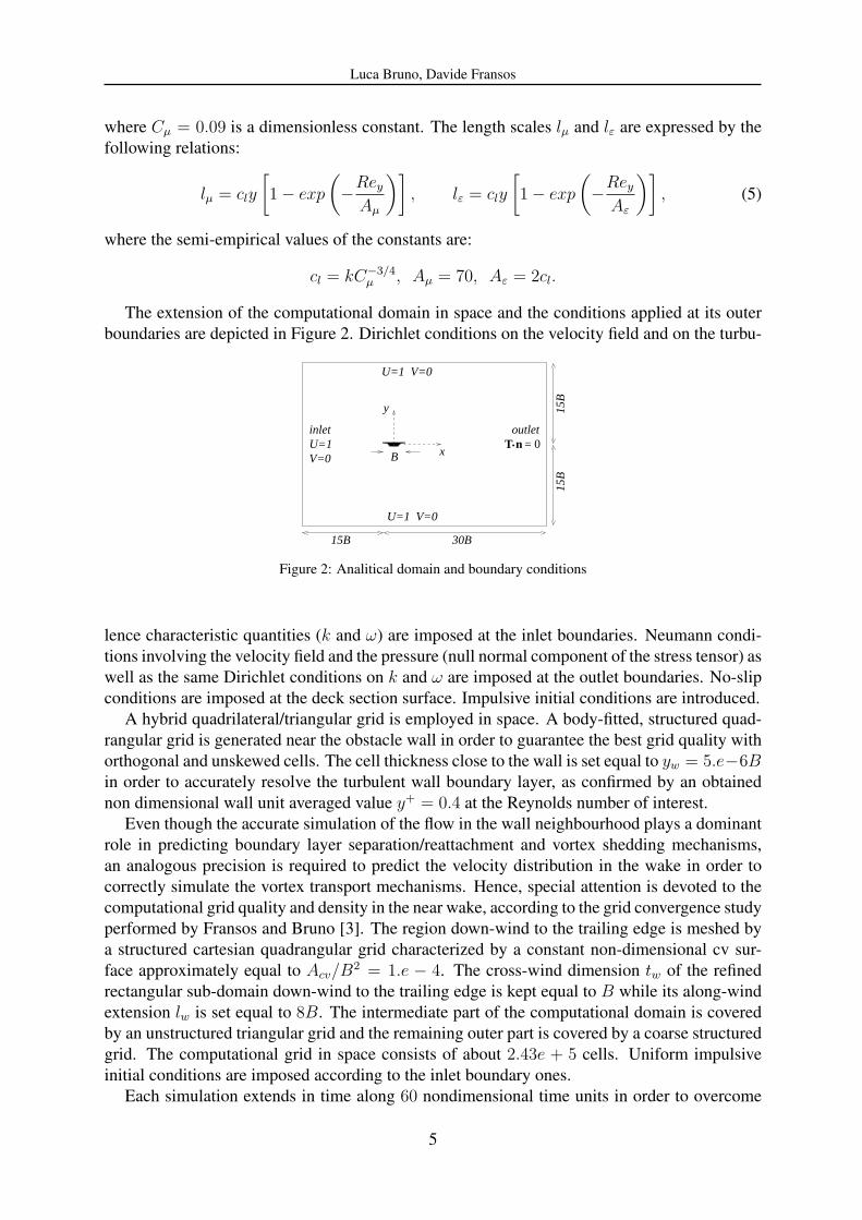
The extension of the computational domain in space and the conditions applied at its outerboundaries are depicted in Figure 2. Dirichlet conditions on the velocity field and on the turbu-

outlet

V=0

U=1 V=0

T n.U=1V=0

inlet

15B

15B

15B

30B

B

y

x= 0

U=1

Figure 2: Analitical domain and boundary conditions

lence characteristic quantities (k and ω) are imposed at the inlet boundaries. Neumann condi-tions involving the velocity field and the pressure (null normal component of the stress tensor) aswell as the same Dirichlet conditions on k and ω are imposed at the outlet boundaries. No-slipconditions are imposed at the deck section surface. Impulsive initial conditions are introduced.

A hybrid quadrilateral/triangular grid is employed in space. A body-fitted, structured quad-rangular grid is generated near the obstacle wall in order to guarantee the best grid quality withorthogonal and unskewed cells. The cell thickness close to the wall is set equal to yw = 5.e−6Bin order to accurately resolve the turbulent wall boundary layer, as confirmed by an obtainednon dimensional wall unit averaged value y+ = 0.4 at the Reynolds number of interest.

Even though the accurate simulation of the flow in the wall neighbourhood plays a dominantrole in predicting boundary layer separation/reattachment and vortex shedding mechanisms,an analogous precision is required to predict the velocity distribution in the wake in order tocorrectly simulate the vortex transport mechanisms. Hence, special attention is devoted to thecomputational grid quality and density in the near wake, according to the grid convergence studyperformed by Fransos and Bruno [3]. The region down-wind to the trailing edge is meshed bya structured cartesian quadrangular grid characterized by a constant non-dimensional cv sur-face approximately equal to Acv/B2 = 1.e − 4. The cross-wind dimension tw of the refinedrectangular sub-domain down-wind to the trailing edge is kept equal to B while its along-windextension lw is set equal to 8B. The intermediate part of the computational domain is coveredby an unstructured triangular grid and the remaining outer part is covered by a coarse structuredgrid. The computational grid in space consists of about 2.43e + 5 cells. Uniform impulsiveinitial conditions are imposed according to the inlet boundary ones.

Each simulation extends in time along 60 nondimensional time units in order to overcome

5


the transient solution due to impulsive initial conditions and to allow the statistic analysis of thesubsequent periodic flow. The nondimensional timestep needed for an accurate advancement intime is ∆t = 0.01.

The Finite Volume solver Fluent is used to numerically evaluate the flowfield. The cell-centre values of the variables are interpolated at face locations using a second-order CentralDifference Scheme for the diffusive terms on all the elements and Quadratic Upwind Interpo-lation for Convective Kinematics and second-order Upwind Scheme for the convection termson quadrilateral and triangular cells, respectively. Advancement in time is accomplished by thesecond-order implicit Euler scheme.

The computations are carried out on a single Intel Xeon X5355 2.66GHz CPU with 2GB ofmemory and they require about 60 hours of CPU time for each simulation.

3 Application to bare deck section

The geometry of the investigated deck section is the same as in Figure 1 and the lower cornercurvature radius R is defined as in Table 1. No aerodynamic appendages or platform equipmentare included in the model. For the sake of simplicity, the dimensionless parameters R/B andLt/B are hereafter notated asR and Lt, respectivelly. It is worth recalling that their investigatedvalues range in the 0.01 ≤ R ≤ 0.05 and 1e − 3 ≤ Lt ≤ 1 intervals. The Reynolds numberis kept constant and equal to ReB = 5.76e + 5 for each simulation, the isotropic turbulenceintensity It = 1% and the angle of attack α = 0.

3.1 R-Lt sensitivity analysis

Figure 3 shows performed computational experiment grid in the R−Lt plane. A total num-ber of 137 computational simulations have been performed, corresponding to about 8220 hoursof CPU time. The point density has been adapted step-by-step during the study in order toproperly describe the local trend of the most significant aerodynamic integral quantities. The

0.01 0.02 0.03 0.04 0.05

0.1

0.2

0.3

0.4

0.5

0.6

0.7

0.8

0.9

1

R

Lt

Figure 3: Grid of the computational experiments

Strouhal number StD and the mean and rms values of the drag and lift coefficients are in par-ticular selected. The StD number is obtained by the Power Spectral Density (PSD) euristic

6


analysis of the flow velocity at the near wake point x/B = 2.5, y/B = 0. The point-wiseobtained results and their best piece-wise polynomial least-square fitting are plotted in Figure4. Four main regions of the investigated R− Lt plane can easily be distinguished, where somecommon features can be recognized in the trend of each quantity.

Strong gradients occur for low values of both the curvature radius and the integral turbu-lence length scale, while smoother variations generally occur at high Lt values. A sudden dropin the mean aerodynamic forces and a corresponding sudden increase in the St number occurat the lowest Lt = 1.e − 3 for increasing radius values. The lift coefficent changes in sign,passing from CL = +0.25 to CL = −0.1, while the St number passes from StD = 0.16 toStD = 0.27: these results are in good qualitative agreement with the ones reported in previousstudies and which are summarized in Table 1. The flow is suspected to be highly unsteady,as the high rms values of the aerodynamic coefficients suggest. The watershed value at whichsuch sudden changes take place has been localized in the narrow 0.02447 ≤ R ≤ 0.02499 rangein conjunction with the adopted flow features. The previously mentioned discontinuity wouldseem to suggest a switch in the overall aerodynamic regime, analogously to what happens inthe individual Re critical regime.

In the intermediate turbulence scale range (0.18 ≤ Lt ≤ 0.3), the flow appears quasi steadyin conjunction with low radius values (R ≤ 0.023), since the drag and lift rms values are almostnull.

The R sensitivity pointed out at low Lt values dramatically reduces at high turbulence scales(Lt ≥ 0.3), where each integral parameter is almost constant when R is varied. Conversely,the Lt sensitivity still remains at high R values, even though smoother variations occur, foreach integral parameter, than at low R values. The first outcome is consistent with what is gen-erally stated about the regularizing and smoothing effect of the incoming turbulence intensityon bluff body aerodynamic behaviour. The second one reveals two qualitativelly different Ltsensitivities, i.e. a discontinuous one and a smooth one, for bodies characterized by high andlow degree-of-bluffness, respectively.

3.2 Aerodynamic regime identification

The trend of the selected integral parameters suggests the necessity of deeply investigatingthe existence of multiple aerodynamic regimes in the R − Lt plane for the same Re number.The computational approach post-processing facilities allow a deeper insight into the mean andinstantaneous flow field around the body. Figure 5 shows the time-averaged x-velocity u1 iso-contours corresponding to null and 0.99 nondimensional values, i.e., it points out the reversedand disturbed flow outer boundaries, respectively. Four R−Lt couples of values are selected toexamine the flow features corresponding to the regions mentioned in the previous section. Thefirst and the third cases correspond to the lowest Lt = 1e− 3 value while R values are chosento be lower and higher than the watershed value at which discontinuity takes place; the secondone is characterized by an Lt in the intermediate range 0.1 ≤ Lt ≤ 0.2 and by low R; the lastone corresponds to the highest Lt = 1 value.

Four regimes are identified and named according to the nomenclature adopted by Schewe[13] concerning the Re effects on a trapezoidal deck because of the analogous observed aerody-namic behaviour. The regimes clearly differ from each other in the position along the upper andlower deck surfaces at which the boundary layer separates and reattaches, as depicted in Figure5(a) by circles and triangles, respectively:

• sub-critical regime (low St, high mean and rms drag and lift values), long separation

7


St

CD

CL

CDRMS

CLRMS

R

Lt

0.01 0.02 0.03 0.04 0.05

0.1

0.2

0.3

0.4

0.5

0.6

0.7

0.8

0.9

1

0.16

0.18

0.2

0.22

0.24

0.26

0.28

R

Lt

0.01 0.02 0.03 0.04 0.05

0.1

0.2

0.3

0.4

0.5

0.6

0.7

0.8

0.9

1

0.08

0.09

0.1

0.11

0.12

0.13

0.14

0.15

0.16

0.17

R

Lt

0.01 0.02 0.03 0.04 0.05

0.1

0.2

0.3

0.4

0.5

0.6

0.7

0.8

0.9

1

−0.1

−0.05

0

0.05

0.1

0.15

0.2

R

Lt

0.01 0.02 0.03 0.04 0.05

0.1

0.2

0.3

0.4

0.5

0.6

0.7

0.8

0.9

1

0.5

1

1.5

2

2.5

3

3.5x 10

−3

R

Lt

0.01 0.02 0.03 0.04 0.05

0.1

0.2

0.3

0.4

0.5

0.6

0.7

0.8

0.9

1

0.005

0.01

0.015

0.02

0.025

0.03

0.035

0.04

Figure 4: Trend of the aerodynamic coefficients

8


bubble at the upper surface, separated flow at the lower surface without reattachment;

• critical regime (large variations of the St number and of the mean drag and lift coeffi-cients, almost null rms values), short separation bubble at the upper surface, long separa-tion bubble at the lower surface due to boundary layer reattachment along the flat plate;

• super-critical regime (high St, low mean drag and lift values), short separation bubble atthe upper surface, the boundary layer separation at the lower surface occurs at the trailingrounded edge;

• trans-critical regime (high St, high mean and low rms drag and lift values), the boundarylayer separation at both the lower and upper surfaces occurs at the trailing edges.

Generally speaking, it is worth pointing out that local changes in the lower edge radius of cur-vatureR involve not only local effects on the lower surface separation bubble, but also non localones on the upper surface separation bubble, on the vortex shedding mechanism and finally onthe overall aerodynamic deck behaviour.

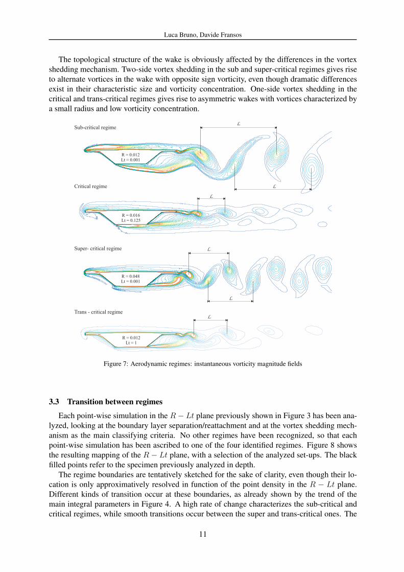
The near wake mean crosswind extension significantly varies in the four regimes, as shownin Figure 5(b). This flow feature, in conjunction with the large Stouhal number variations, sug-gests that different vortex shedding mechanisms occur in the identified regimes. The mean andrms x-velocity profiles along the x/B = 0.55 and x/B = 1.0 straights (see Figure 5(b)) areplotted in Figure 6. The mean x-velocity profile points out slight differences in both the max-imum velocity defect and its location along the reference straights. In particular, the massiveseparation at the lower surface in the sub-critical regime drops the maximum velocity defect ab-scissa below y = 0. The rms x-velocity profile along the x/B = 0.55 straight reveals dramaticdifferences in the fluctuating flow field for the regimes: the sub-critical and the super-criticalones show two local peaks, the trans-critical one is characterized by only one peak in correspon-dence to the upper trailing edge, while the critical one involves negligible x-velocity fluctuationsjust downwind to the upper trailing edge. In the critical regime, the x-velocity fluctuations de-velop more downwind to the upper trailing edge, as shown in the rms x-velocity profile alongthe x/B = 1.0 straight. A more evident physical meaning of the above described profiles isprovided in Figure 7, where the instantaneous vorticity magnitude isocontours correspondingto local maxima in the CL time history are plotted for the four regimes. The relative distancebetween two successive vortices shed by the same edge L ∝ St−1 is depicted.The vortex shedding mechanism mainly distinguishes two classes of regimes. On one hand, thesub and super-critical ones, i.e., the ones defined for a low turbulence length scale, are character-ized by vortex shedding from both the upper and lower edges. Neverthless, it is worth recallingthat vortices at the lower surface are shed at the leading edge in the sub-critical regime, whilevortex shedding from the trailing edge takes place in the super-critical regime. On the otherhand, the critical and trans-critical regimes only involve significant vortex shedding from theupper trailing edge. Neverthless, the point at which the upper vortices are shed in the wake ismore downwind located in the critical regime rather than in the trans-critical one. It is worthpointing out that the x/B = 0.55 straight is upwind to the vortex shedding point in the criticalregime, so that the extremely low values in the x-velocity rms profile (Figure 6) are justified.Bearing in mind that vortices are shed downwind in the wake in the critical regime, their con-tribution to the aerodynamic force fluctuating component is expected to be small in the criticalregime. This flow feature can help explain the almost null lift and drag rms valus in this regime(Figure 4).

9


Figure 5: Aerodynamic regimes: null (a) and .99 (b) mean x-velocity isocontours

Figure 6: Mean (a) and RMS (b) horizontal velocity at x/B = 0.55

10


The topological structure of the wake is obviously affected by the differences in the vortexshedding mechanism. Two-side vortex shedding in the sub and super-critical regimes gives riseto alternate vortices in the wake with opposite sign vorticity, even though dramatic differencesexist in their characteristic size and vorticity concentration. One-side vortex shedding in thecritical and trans-critical regimes gives rise to asymmetric wakes with vortices characterized bya small radius and low vorticity concentration.

Figure 7: Aerodynamic regimes: instantaneous vorticity magnitude fields

3.3 Transition between regimes

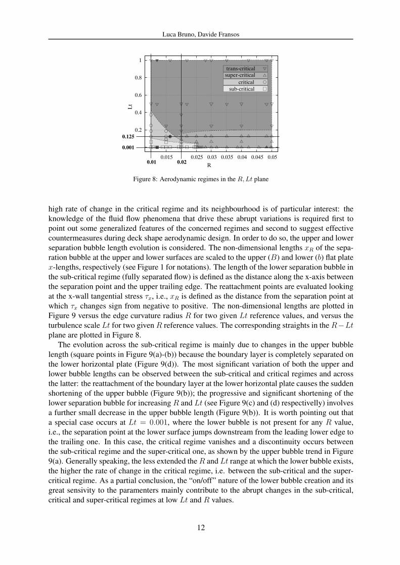
Each point-wise simulation in the R− Lt plane previously shown in Figure 3 has been ana-lyzed, looking at the boundary layer separation/reattachment and at the vortex shedding mech-anism as the main classifying criteria. No other regimes have been recognized, so that eachpoint-wise simulation has been ascribed to one of the four identified regimes. Figure 8 showsthe resulting mapping of the R − Lt plane, with a selection of the analyzed set-ups. The blackfilled points refer to the specimen previously analyzed in depth.

The regime boundaries are tentatively sketched for the sake of clarity, even though their lo-cation is only approximatively resolved in function of the point density in the R − Lt plane.Different kinds of transition occur at these boundaries, as already shown by the trend of themain integral parameters in Figure 4. A high rate of change characterizes the sub-critical andcritical regimes, while smooth transitions occur between the super and trans-critical ones. The

11


Figure 8: Aerodynamic regimes in the R,Lt plane

high rate of change in the critical regime and its neighbourhood is of particular interest: theknowledge of the fluid flow phenomena that drive these abrupt variations is required first topoint out some generalized features of the concerned regimes and second to suggest effectivecountermeasures during deck shape aerodynamic design. In order to do so, the upper and lowerseparation bubble length evolution is considered. The non-dimensional lengths xR of the sepa-ration bubble at the upper and lower surfaces are scaled to the upper (B) and lower (b) flat platex-lengths, respectively (see Figure 1 for notations). The length of the lower separation bubble inthe sub-critical regime (fully separated flow) is defined as the distance along the x-axis betweenthe separation point and the upper trailing edge. The reattachment points are evaluated lookingat the x-wall tangential stress τx, i.e., xR is defined as the distance from the separation point atwhich τx changes sign from negative to positive. The non-dimensional lengths are plotted inFigure 9 versus the edge curvature radius R for two given Lt reference values, and versus theturbulence scale Lt for two givenR reference values. The corresponding straights in theR−Ltplane are plotted in Figure 8.

The evolution across the sub-critical regime is mainly due to changes in the upper bubblelength (square points in Figure 9(a)-(b)) because the boundary layer is completely separated onthe lower horizontal plate (Figure 9(d)). The most significant variation of both the upper andlower bubble lengths can be observed between the sub-critical and critical regimes and acrossthe latter: the reattachment of the boundary layer at the lower horizontal plate causes the suddenshortening of the upper bubble (Figure 9(b)); the progressive and significant shortening of thelower separation bubble for increasing R and Lt (see Figure 9(c) and (d) respectivelly) involvesa further small decrease in the upper bubble length (Figure 9(b)). It is worth pointing out thata special case occurs at Lt = 0.001, where the lower bubble is not present for any R value,i.e., the separation point at the lower surface jumps downstream from the leading lower edge tothe trailing one. In this case, the critical regime vanishes and a discontinuity occurs betweenthe sub-critical regime and the super-critical one, as shown by the upper bubble trend in Figure9(a). Generally speaking, the less extended theR and Lt range at which the lower bubble exists,the higher the rate of change in the critical regime, i.e. between the sub-critical and the super-critical regime. As a partial conclusion, the “on/off” nature of the lower bubble creation and itsgreat sensivity to the paramenters mainly contribute to the abrupt changes in the sub-critical,critical and super-critical regimes at low Lt and R values.

12


(a) (b)

(c) (d)

Figure 9: Length of the separation bubble

Finally, the separation bubbles at both the upper and lower surfaces show low or null R andLt sensitivities along the super-critical and trans-critical regimes: the mean pressure distribu-tion along the upwind canilever and the vortex shedding mechanism past the downwind one areconfirmed as the main parameters that affect the smooth transition between these regimes.

4 Application to an actual deck aerodynamic design

Bridge designers usually make an attempt to avoid deck shapes that are prone to changesin aerodynamic regimes in order to face well determined design wind loads. Hence, quasi-streamlined or bluff sections are preferred to the ones characterized by an intermediate degree-of-bluffness. Both streamlining and bluffness can be obtained, during the design phase or as aretrofitting measure, by means of aerodynamic appendages, e.g. rounded fairings, sharpeningwedges and guide vanes, if the deck chord-to-width B/D and the upper-to-lower flat plate B/bratios are imposed by structural needs. The aim of this section is to verify the effectivenessof some of these appendages, referring to the same deck section and the same incoming flowconditions investigated above. To do so, the Sunshine Bridge deck section with sharpeningaerodynamic appendages at its lower edges (see Table 1), as tested in the wind tunnel by Ric-ciardelli and Hangan [11], is subjected to a sensitivity analysis to the turbulence length scale.The same previously explored Lt range (1e − 3 ≤ Lt ≤ 1) is sampled with a coarse grid(∆log(Lt) ≈ 1). The obtained results are summarized in Table 2.

The results clearly show that, even for the sharpest and the smoothest edge treatment, i.e., forthe highest and smallest degree-of-bluffness, it is not possible to assure a unique aerodynamic

13


Table 2: Integral length scale sensitivity for the wind tunnel geometry

corner inflow conditions St CL u1/U = 0 regime

It = 1%, Lt = 1e−3 0.131 0.406 subcritical



It = 1%, Lt = 1e−0 steady 0.252 critical

regime at each turbulence scale.The boundary layer at the lower surface is forced to separate by the leading edge sharpen-

ing at each length scale, so that the occurence of the super-critical and trans-critical regimes isavoided. In the Lt ≤ 0.1 range, the sub-critical regime occurs analogously to what happens forthe bare section, even though some peculiarities arise: the reattachment point is located alongthe trailing cantilever lower surface and the recirculation bubble at the upper surface grows toxR/B ≈ 0.5 at the smallest length scale. On the contrary, at Lt = 1, the boundary layer at thelower surface reattaches to the horizontal plate so that the deck aerodynamics switches from thesub-critical regime to the critical one. In other words, from a designer’s point of view, the intro-duction of sharping appendages does not prevent the occurrence of two qualitatively differentforms of aerodynamic behaviour, characterized by significant changes in wind loads.

The mean and rms pressure coefficient distribution around the deck with sharpening ap-pendages at various Lt values are plotted in Figure 10 and compared with the Ricciardelli andHangan [11] experimental data. The experimental data lie between the computational curves,and more precisely around the ones referring to 0.01 ≤ Lt ≤ 0.1, which is supposed to bethe Lt range generated in the wind tunnel by Ricciardelli and Hangan [11], except for the rmspressure coefficient distribution along the upper surface. In this case, the poor agreement can beascribed to computational errors due to turbulence modelling or to the numerical approach, butthe sensitivity to further small differences between the experimental and computational set-ups,e.g. in turbulence intensity, cannot be excluded a priori.

The obtained results suggest that the aerodynamic loads resulting from the so-called “smoothincoming flow” conditions, i.e. residual turbulence intensity and undefined turbulence lengthscale, should be handled with care because of non negligible uncertainty effects even for high orlow deck degree-of-bluffness. The use of accurate evaluation of the turbulence intensity and asensitivity analysis to the generated turbulence length scale seems to be proper method to guar-antee a correct comparison of the results from different experimental facilities and to proposea wide range of wind load scenarios to designers. Finally, it is worth pointing out that, at leastfor this benchmark, the computational approach shows an analogous level of accuracy to theexperimental one.

14


Figure 10: Mean and RMS pressure coefficient distribution for different inflow conditions - Sharping appendages

5 Conclusions

In this paper, the edge degree-of-sharpness and free-stream turbulence scale effects on theaerodynamics of a trapezoidal bridge deck have been systematically addressed by means ofa computational approach. The aerodynamic coefficients show a dramatic sensitivity to theseparameters. The results have been analyzed in terms of mean and instantaneous flow fields,looking at both global and local fluid flow phenomena. The obtained results clearly confirmthat the individual regimes proposed to classify the Reynolds number effects on bluff bodiescan be further generalized to the aerodynamic effects of other set-up parameters, and character-ized by the boundary layer separation and reattachment around a given bluff body. Furthermore,the results show that the shift from regime to regime can be driven not only by the overall in-coming flow features, such as the Re number or the turbulence length scale, but also by localand small changes in the body shape. Finally, the sensitivity analysis to the turbulence scale hasbeen applied to the actual extreme design solution obtained with sharpening aerodynamic ap-pendages. Neither deck shape is capable of preventing switching from an aerodynamic regimeto another one.

Acknowledgements

The authors wish to thank Prof. F. Ricciardelli and Dr. C. Mannini for kindly providingthe geometrical properties of the Sunshine Skyway Bridge and the wind-tunnel test set-up data.Further thanks go to Dr. S. Khris for the helpful discussions about the topics of the paper.The financial support provided by the Italian Ministry of Education, University and ResearchM.I.U.R. within the project “Aeroelastic phenomena and other dynamic interaction on non-conventional bridges and footbridges” is gratefully acknowledged.

15


References

[1] H. Chen and V. Patel. Near-wall turbulence models for complex flows including separa-tion. AIAA Journal, 26(6), 641–648, 1988.

[2] N. K. Delany and N. E. Sorensen. Low-speed drag of cylinders of variuos shapes. NACATN 3038, 1953.

[3] D. Fransos and L. Bruno. Determination of the aeroelastic transfer functions for stream-lined bodies by means of a navier-stokes solver. Mathematical and Computer Modelling,43, 506–529, 2006.

[4] A. Laneville and C. Williams. The effects of intensity and large scale turbulence on themean pressure and drag coefficients of 2d rectangular cylinders. Proc. 5th Int. Conferenceon Wind Effects on Building and Structures, Fort Collins, Colorado, July 8-14, 1979.

[5] G. Larose and A. D’Auteuil. On the reynolds number sensitivity of the aerodynamics ofbluff bodies with sharp edges. Journal of Wind Engineering and Industrial Aerodynamics,94, 365–376, 2006.

[6] Q. Li and W. Melbourne. An experimental investigation of the effects of free-streamturbulence on streamwise surface pressures in separated and reattaching flows. Journal ofWind Engineering and Industrial Aerodynamics, 54/55, 313–323, 1995.

[7] C. Mannini. Flutter Vulnerability Assessment of Flexible Bridges. PhD thesis, Universityof Florence - Technische Universitat Carolo-Wilhelmina zu Braunschweig, 2006.

[8] C. Mannini. Personal communication. 2007.

[9] C. Mannini, A. Soda, and R. Voß. Computational investigation of flow around bridgesections. pages 343–350, Dubrovnik, Croatia, 2006.

[10] Y. Nakamura and S. Ozono. The effects of turbulence on a separated and reattaching flow.Journal of Fluid Mechanics, 178, 477–490, 1987.

[11] F. Ricciardelli and H. Hangan. Pressure distribution and aerodynamic forces on stationarybox bridge sections. Wind and Structures, 4(5), 399–412, 2001.

[12] A. Roshko. Experiments on the flow past a circular cylinder at very high reynolds number.Journal of Fluid Mechanics, 10, 345–356, 1961.

[13] G. Schewe. Reynolds-number effects in flow around more-or-less bluff bodies. Journal ofWind Engineering and Industrial Aerodynamics, 89, 1267–1289, 2001.

[14] G. Schewe and A. Larsen. Reynolds number effects in the flow around a bluff bridge deckcross section. Journal of Wind Engineering and Industrial Aerodynamics, 74-76, 829—838, 1998.

[15] T. Tamura and T. Miyagi. The effect of turbulence on aerodynamic forces on a squarecylinder with various corner shapes. Journal of Wind Engineering and Industrial Aerody-namics, 83, 135–145, 1999.

[16] D. Wilcox. Turbulence Modelling for CFD. DCW Industries Inc., La Canada, California,1998.

16

EDGE DEGREE-OF-SHARPNESS AND INTEGRAL LENGTH SCALE EFFECTS...

Documents

Transcript of EDGE DEGREE-OF-SHARPNESS AND INTEGRAL LENGTH SCALE EFFECTS...