ECOTONE PROPERTIES AND INFLUENCES ON FISH DISTRIBUTIONS ALONG
141
ECOTONE PROPERTIES AND INFLUENCES ON FISH DISTRIBUTIONS ALONG HABITAT GRADIENTS OF COMPLEX AQUATIC SYSTEMS A Dissertation Presented to the Faculty of the Graduate School of Cornell University In Partial Fulfillment of the Requirements for the Degree of Doctor of Philosophy by Nuanchan Singkran May 2007
Transcript of ECOTONE PROPERTIES AND INFLUENCES ON FISH DISTRIBUTIONS ALONG

ECOTONE PROPERTIES AND INFLUENCES ON FISH DISTRIBUTIONS
ALONG HABITAT GRADIENTS OF COMPLEX AQUATIC SYSTEMS
A Dissertation
Presented to the Faculty of the Graduate School
of Cornell University
In Partial Fulfillment of the Requirements for the Degree of
Doctor of Philosophy
by
Nuanchan Singkran
May 2007

© 2007 Nuanchan Singkran
ECOTONE PROPERTIES AND INFLUENCES ON FISH DISTRIBUTIONS
ALONG HABITAT GRADIENTS OF COMPLEX AQUATIC SYSTEMS
Nuanchan Singkran, Ph. D.
Cornell University 2007
Ecotone properties (formation and function) were studied in complex aquatic
systems in New York State. Ecotone formations were detected on two embayment-
stream gradients associated with Lake Ontario during June–August 2002, using abrupt
changes in habitat variables and fish species compositions. The study was repeated at
a finer scale along the second gradient during June–August 2004. Abrupt changes in
the habitat variables (water depth, current velocity, substrates, and covers) and peak
species turnover rate showed strong congruence at the same location on one gradient.
The repeated study on the second gradient in the summer of 2004 confirmed the same
ecotone orientation as that detected in the summer of 2002 and revealed the ecotone
width covering the lentic-lotic transitions. The ecotone on the second gradient acted
as a hard barrier for most of the fish species. Ecotone properties were determined
along the Hudson River estuary gradient during 1974–2001 using the same methods
employed in the freshwater system. The Hudson ecotones showed both changes in
location and structural formation over time. Influences of tide, freshwater flow,
salinity, dissolved oxygen, and water temperature tended to govern ecotone properties.
One ecotone detected in the lower-middle gradient portion appeared to be the optimal
zone for fish assemblages, but the other ecotones acted as barriers for most fish
species.
A spatially explicit abundance exchange model (AEM) was developed to predict

distribution patterns of five fish species in relation to their population characteristics
and habitat preferences across the lentic-lotic ecotones on the two freshwater gradients
associated with Lake Ontario. Preference indexes of each target fish species for water
depth, water temperature, current velocity, cover types, and bottom substrates were
estimated from field observations, and these were used to compute fish habitat
preference (HP). Fish HP was a key variable in the AEM to quantify abundance
exchange of an associated fish species among habitats on each study gradient. The
AEM efficiently determined local distribution ranges of the fish species on one
gradient. Results from the model validation showed that the AEM was able to
quantify most of the fish species distributions on the second gradient.

iii
BIOGRAPHICAL SKETCH
Nuanchan Singkran was born in Chantaburi province located in the eastern part of
Thailand. After finishing high school, Nuanchan entered the faculty of Science at
Chulalongkorn University in 1989 for her undergraduate study in Marine Science with
a major in Marine Biology. Study at the Marine Science Department allowed her to
obtain broad knowledge of both applied science and ecology, especially the
relationship between aquatic creatures and environmental conditions along the coastal
zone of Thailand. After graduation, Nuanchan began her career as an environmental
reporter for Thai and English newspapers during 1993–1996. During her career as a
journalist, Nuanchan received a 2nd place award for an environmental article
supporting Eco-Tourism of Thailand in 1993, and the award for outstanding
environmental news reporter from the Environmental Siam Association in 1994.
Nuanchan’s work in the media provided her a unique opportunity to observe various
environmental problems in Thailand. She realized that the deterioration of natural
resources in the country comes primarily from public lack of understanding and
awareness about the environment. Lack of suitable methodologies to solve problems
and weak environmental policy are additionally significant factors that aggravate
environmental problems. Although Nuanchan likes the challenge of media work, she
needed to be engaged more actively in the problem-solving process. She believed that
academic and research work is really the area that would allow her to contribute to
public education and in-depth research on specific issues.
During 1996–1999, Nuanchan obtained scholarships from the Chin Sophonpanich
Foundation for Environment and from the Biodiversity Research Grant to further her
Master’s program in the multidisciplinary Department of Environmental Science,
Chulalongkorn University. Her Master’s thesis was entitled “Species Composition of
iv
Fish in Mangrove Canals as Reflected from Coastal Land Use at Trat Bay, Thailand”.
Her interest in this topic comes from the fact that a large number of fish species (over
2,000 across the country) have been seriously threatened by human activities,
especially the conversion of coastal areas into shrimp farms, urban districts, or
industrial zones, all done without proper management. Her Master’s research using
fish as a biological indicator revealed that improper land use activities altered the
coastal environment, which in turn affected fish and other living communities in
coastal systems in terms of both abundance and species diversity. After completing
her Master’s degree, Nuanchan received a government scholarship to pursue her PhD
program in Natural Resources at Cornell University in Ithaca, New York in 2001. At
Cornell, Nuanchan conducted her dissertation research on influences of ecotone
properties (formation and function) on species distributions over spatial and temporal
scales. Her research work dealt with both empirical and simulation modeling to
determine ecotone formation in complex aquatic systems and ecotone function on fish
species assemblages. Additionally, she used a simulation model to spatially and
temporally forecast distribution of fish species assemblages across aquatic boundaries.

v
For all fish and other creatures across global boundaries

vi
ACKNOWLEDGMENTS
My graduate committee played vital roles throughout the development of my
dissertation research. I am grateful to all of them for giving me the chance to freely
design and follow my research ideas. My committee Chair, Dr. Mark B. Bain, not
only supported me in any situation during my PhD program at Cornell University, but
also shared his philosophy of thinking and was patient in shaping my research work to
continue on the right track. Without his strong academic support and other help, my
graduate study at Cornell University could not have been completed. As one of my
committee, Dr. Patrick J. Sullivan always gave me instructive comments and helpful
suggestions that greatly improved the quality of my research work. His simple
questions, e.g., “Why is an ecotone is important?” and “How many functions can an
ecotone have?” caused me to think deeply, carefully, and quantitatively on my ecotone
study. Prof. Daniel P. Loucks is not just one of my committee, but also one of the best
teachers I have ever had during my lifetime as a student. Although Prof. Loucks said
that he did not know anything about fish and ecology, his contributions to my research
work deserve praise. Following his suggestion to take some core courses in his
department of Civil and Environmental Engineering, I gained more modeling
experience and recovered my mathematical background to achieve my dissertation
research.
The Royal Thai Government and Thai people whose tax money supported me to
study in the USA deserve any credit for my accomplishments. Additionally, my
special thanks are due to the Lake Ontario Biocomplexity Project (Natural Science
Foundation OCE–0083625), the Hudson River Foundation (GF/01/05), and the
College of Agriculture and Life Sciences at Cornell University, which partly
supported my study and research. I thank Prof. Paul A. Delcourt and Prof. Hazel R.

vii
Delcourt for suggesting ecotone analysis; John Young from ASA Analysis &
Communication, Inc. for providing the beach seine fish and habitat data from the
Utilities’ Hudson River estuary monitoring program; John Ladd from New York State
Department of Environmental Conservation for providing the substrate and shoreline
data; and the Cornell University’s Geospatial Information Repository for providing
submerged aquatic vegetation data.
The completion of my graduate program at Cornell University would be
impossible without the warm support and encouragement from friends and
collaborators. I am thankful to Kristi Arend, Takao Kumazawa, Kathy Mills, James
Murphy, Marci Meixler, Emelia Deimezis, Geof Eckerlin, Gail Steinhart, Carol
Steinhart, Geoff Steinhart, and all the other people I cannot name here for their
support and help during my study period at Cornell. I thank my parents and my
husband, Poonrit Kuakul, for their patience and understanding. I am thankful to my
senior friends, Dolina Millar, Bruce Anderson, Wandee Anderson, and some sisters
and brothers from the Taste of Thai restaurant who made my life in Ithaca not so
lonely and never refused to help me in any manner they could.

viii
TABLE OF CONTENTS
Biographical sketch iii
Dedication v
Acknowledgments vi
List of figures ix
List of tables xii
Chapter One Ecotone properties in the freshwater system associated 1 with Lake Ontario, New York.
Chapter Two Ecotone properties in the Hudson River estuary system 26 New York.
Chapter Three An abundance exchange model of fish assemblage 60 response to changing habitat along embayment-stream gradient of Lake Ontario, New York.
Appendix 2.1. Cumulative abundance and species richness of fish 93 by region (RE) along the Hudson River estuary gradient (RE1–RE12) from the five power plant utilities’ Hudson River estuary monitoring program using beach seine survey during 1974 to 2001.
Appendix 2.2. Multiple functions (aggregator, mediator, soft barrier, 105 and hard barrier) of the ecotones (from all frequencies of detection) on the Hudson fish species in each time period during 1974–2001.
Appendix 2.3. Multiple functions (neutral, partly inhibit, and 109 completely inhibit) of the ecotone peripheries (from all frequencies of detection) on the Hudson fish species in each time period during 1974–2001.
References 112
ix
LIST OF FIGURES
Figure 1.1. Ecotone structures and functions. 5
Figure 1.2. Sampling stations along the Sterling gradient during the 9
summer of 2002 (June–August). Observed value of each habitat variable was averaged over the three summer months and compared among stations using different sizes (small, medium, large) of bar charts to display mean magnitude (low, intermediate, or high).
Figure 1.3. Sampling stations along the Floodwood gradient during the 11
summer of 2002 (June–August). Observed value of each habitat variable was averaged over the three summer months and compared among stations using different sizes (small, medium, large) of bar charts to display mean magnitude (low, intermediate, or high).
Figure 1.4. Twelve stations (rectangles) were sampled along the 13
Floodwood gradient in the summer of 2004 (June–August) compared to the eight stations (circles) sampled in the summer of 2002. The ecotone periphery was indicated monthly by a peak absolute difference in the beta diversity (δ beta A) of fish species (June = connected line, July = dashed line, and August = gray line with squared marker) in each study summer.
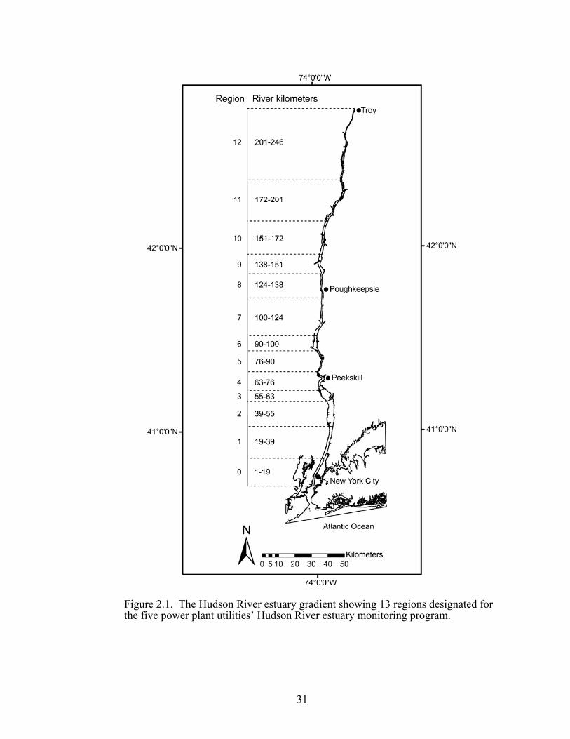
Figure 2.1. The Hudson River estuary gradient showing 13 regions 31
designated for the five power plant utilities’ Hudson River estuary monitoring program.
Figure 2.2. Frequency of ecotones detected monthly based on the 39
data collection along the Hudson River estuary gradient during 1974–2001.
Figure 2.3. Ecotones (thick bars) and ecotone peripheries (thick lines) 40
detected during 1974–2001on the Hudson River estuary gradient covering 228 river kilometers (RKM) from region (RE) 1 to RE12 are grouped into each frequency class. Numbers of times of the formation of an ecotone and an ecotone periphery in each location are shown in brackets in each frequency class on the right side of the graph.

x
Figure 2.4. Monthly mean values of dissolved oxygen observed along 47 the Hudson River estuary gradient in the detected ecotone (line with solid dot markers) and non-detected ecotone (line with open dot markers) periods.
Figure 2.5. Monthly mean values of salinity observed along the 49
Hudson River estuary gradient in the detected ecotone (line with solid dot markers) and non-detected ecotone (line with open dot markers) periods.
Figure 2.6. Monthly mean values of water temperature observed 50
along the Hudson River estuary gradient in the detected ecotone (line with solid dot markers) and non-detected ecotone (line with open dot markers) periods.
Figure 2.7. Values of dissolved oxygen (DO), salinity, and water 52
temperature were averaged by region over the 116 time periods that the ecotones were detected. Bed areas of two submerged aquatic vegetation (SAV) species (Trapa natans and Vallisneria american) vary along the gradient (data for region 1 were unavailable). Proportions of 10 substrate types were observed in the tidal river estuary.
Figure 3.1. The Floodwood (FL) and Sterling (ST) gradients with eight 65
sampling stations (stars, FL; circles, ST) for monthly collecting of target fish and habitat variables during June–August 2002. The fish and habitat collections were repeated at 12 stations (circles) along the FL gradient during June–August 2004.
Figure 3.2. A conceptual diagram of fish distribution within and among 70
habitats. Migration rates of fish at two life stages in the growing season (yk, 0+ yr old; ak, 1+ yr old) and for all fish in winter (k) among habitats n, n–1, and n+1 are dependent on fish habitat preference in the growing season (yHP, 0+ yr old; aHP, 1+ yr old) and in winter (HP), respectively.
Figure 3.3. Categorized mean values of all habitat variables (except 77
substrate composition) observed monthly during June–August 2002 along the Floodwood gradient.
Figure 3.4. Categorized mean values of all habitat variables (except 79
substrate composition) observed monthly during June–August 2002 along the Sterling gradient.

xi
Figure 3.5. Seasonal distribution pattern of yellow perch over the 81 100-year simulation (A). The fish population size exponentially decreased or increased for the first 10-year period of the simulation when changes of 50% of carrying capacity Cy (B), birth fraction rb (C), or death fraction rd (D) were assigned to the abundance exchange model, but the population size returned to the seasonal pattern over the long-term prediction.
Figure 3.6. Observed abundances of yellow perch (YP), bluegill (BG), 83
bluntnose minnow (BM), logperch (LP), and fantail darter (FTD) along the Floodwood gradient in August 2004 were compared with the mean predicted abundance ± standard deviation of the prediction of the associated fish species in August over the 100-year simulation.
Figure 3.7. Mean predicted abundance of yellow perch (YP), bluegill 85
(BG), bluntnose minnow (BM), logperch (LP), and fantail darter (FTD) among months and stations on the Floodwood gradient over the 100-year simulation.
Figure 3.8. Observed abundance of yellow perch (YP), bluegill (BG), 86
bluntnose minnow (BM), and fantail darter (FTD) along the Sterling gradient in August 2002 were compared with the mean predicted abundance ± standard deviation of the prediction of the associated fish species in August over the 100-year simulation.
Figure 3.9. Mean predicted abundance of yellow perch (YP), bluegill (BG), 88
bluntnose minnow (BM), and fantail darter (FTD) among months and stations on the Sterling gradient over the 100-year simulation.

xii
LIST OF TABLES
Table 1.1. Intensity of each habitat variable was average the three 17
summer months (June–August) of 2002 along the Sterling and Floodwood gradients.
Table 1.2. Relative abundance comparison of each fish species 20
among the downstream (DW, FL1–FL3), ecotonal (ECO, FL4–FL5), and upstream (UP, FL6–FL12) habitats on the Floodwood gradient over the summer months of 2004 (June–August).
Table 2.1. Functions of the ecotones detected ≥5 times at certain 41
regions (RE) and time periods on Hudson fish species assemblages.
Table 2.2. Functions of the ecotone peripheries detected ≥5 times 43
at certain regions (RE) and time periods on Hudson fish species assemblages.
Table 2.3. Results from multivariate analysis of variance for each 46
habitat variable and its delta (absolute difference between minimum and maximum values) between non-detected (ECO = 0) and detected (ECO = 1) ecotone periods and due to the interactions of ECO × RE (river region), ECO × Month, ECO × Year, ECO × RE × Month, ECO × RE × Year, and ECO × Month × Year.
Table 3.1. Initial values of the population variables (Cy, rb, and rd) 73
and individuals of each target fish species for simulating the abundance exchange model.
Table 3.2. Preference index (Pi) for each habitat variable of five 75
modeled fish species at two life stages (0+yr and 1+yr old) estimated from the fish and habitat data observed along the Floodwood gradient over the three summer months (June–August) of 2004.

1
CHAPTER ONE
Ecotone properties in the freshwater system associated with Lake Ontario, New York
ABSTRACT
Ecotone formations were detected on two embayment-stream gradients associated
with Lake Ontario using abrupt changes in habitat variables and peak turnover rates in
fish species compositions along the gradients. The study was conducted on both
gradients over the three summer months (June–August) of 2002, and it was repeated at
a finer scale along the second gradient over the same summer months of 2004. The
results revealed that the ecotones were static in their orientations on both gradients
during the study periods. In the summer of 2002, abrupt changes in the habitat
variables (water depth, current velocity, substrates, and covers) and peak species
turnover rate showed strong congruence at the same location on one of the two
gradients. On the second gradient, only the peak species turnover rate could clearly
define the ecotone periphery, whereas the abrupt changes in the habitat variables
occurred at multiple locations. The repeated study at the finer scale on the second
gradient in the summer of 2004 confirmed the same ecotone orientation as that
detected in the summer of 2002 and revealed the ecotone width covering the lentic-
lotic transition. Four ecotone functions (aggregator, mediator, soft barrier, and hard
barrier) were inferred from the comparison of relative abundance of fish species
among downstream, ecotonal, and upstream habitats. In general, the ecotone acted as
a hard barrier for most of the fish species. The distinct physical discontinuities below
and above the ecotonal habitat appear to be an important factor shaping the ecotone
geometry and impeding fish distribution into the ecotone.
2
INTRODUCTION
The ecotone concept is almost as old as the field of ecology (Zalewski et al. 2001)
although ecologists have used the concept loosely on a broad range of boundary
conditions. This practice has impeded the development of theory and the recognition
of patterns that could advance the understanding and use of the ecotone idea (Strayer
et al. 2003). Nevertheless, ecotone studies in ecosystems have remained prominent
and appealing (e.g., Clements 1897, Leopold 1933, Odum 1971, Risser 1990, Johnson
et al. 1992, Winemiller and Leslie 1992, Lidicker 1999, Fortin et al. 2000, Willis and
Magnuson 2000, Harding 2002, Cadenasso et al. 2003, Martino and Able 2003, Miller
and Sadro 2003, Ries et al. 2004) because of the important roles of ecotones on
biodiversity (di Castri and Hansen 1992, Neilson et al. 1992, Lachavanne 1997), biotic
interactions (Wiens et al. 1993), flows of materials and nutrients in ecosystems
(Hansen and di Castri 1992), and the ecological implications for natural resources
management at the individual, population, and ecosystem levels (Sisk and Haddad
2002).
Clements (1897) was the first who viewed an ecotone as the transition zone
between different plant communities. He observed that the vegetation in this zone was
often accentuated in size and density. Leopold (1933) later explained that shape and
spatial configuration of an ecotone influence species richness and organism
abundance. Successive ecotone studies (e.g., Lay 1938, Johnston and Odum 1956)
worked with these early ideas. Odum (1971) defined an ecotone as a transition zone
between two or more communities, and he labeled the increases in both species
richness and abundance at the ecotone as a consequence of the “edge effect”. At
present, an ecotone is widely viewed as a transition zone between adjacent ecological
systems with influences on organism distributions going beyond the traditional “edge

3
effect” (e.g., Holland 1988, Naiman and Décamps 1990, Fortin et al. 2000, Fagan et
al. 2003, Strayer et al. 2003).
From over 900 empirical ecotone studies in terrestrial ecosystems (Ries et al.
2004), ecotones provide diverse influences on abundance distributions of organisms in
and around the ecotones. For instance, results from bird communities (Sisk and
Margules 1993, Baker et al. 2002, Watson et al. 2004) showed that the expected
increase in density and species richness in ecotones was not easily detected because
bird species responded differently, i.e., edge avoiders, edge exploiters, and habitat
generalists. Although distinct changes in bird assemblages were observed at an
ecotone, conditions in the ecotone appeared to be neutral to some species. Birds have
been widely used as ecotone response variables in terrestrial ecosystems (Ries et al.
2004) because of their mobility, diversity, and diverse habitat specializations. Fish are
also mobile organisms that often display high diversities in species richness and life
histories and, thus, appear to be an excellent ecotone indicator (Kirchhofer 1995,
Schiemer et al. 1995) in aquatic ecosystems. However, fewer ecotone investigations
have been conducted in aquatic ecosystems (e.g., Przybylski et al. 1991, Willis and
Magnuson 2000, Martino and Able 2003).
Whereas locations of most terrestrial ecotones can be visually identified (e.g., an
ecotone between grassland and forest) before hypothesis testing, it is more difficult to
determine locations of aquatic ecotones. In aquatic ecosystems, environmental
conditions are complex in space and time due to variations in hydrology (Wiens 2002)
and climate-linked seasonal changes that can alter other aquatic habitat variables (e.g.,
water temperature, growth of aquatic plants and algae). Consequently, ecotone
properties (formation and function) in water systems are highly related to system
variability, and they reflect the dynamics of organism assemblages responding to the
environmental changes over space and time.

4
The objectives of this study were thus to detect the ecotone formation on two
embayment-stream gradients and determine the ecotone function on fish species
assemblages. An ecotone is viewed as a dynamic structure in an ecosystem that
constitutes a unique habitat and possibly a unique community (Fagan et al. 2003). In
this study, it is defined as a zone of transition in the physicochemical properties and
interactions among habitats and species. An ecotone may form, decline, disappear,
shift location, or change in structure or function due to the influence of changing
physicochemical conditions, species use of habitat, and interactions among species
(Holland 1988, Delcourt and Delcourt 1992, Wiens 1992, Kolasa and Zalewski 1995).
Relevant hypotheses and aquatic ecotone studies
The status of an ecotone may differ depending on the spatial scale considered and
the prior delineation of the system of interest (Kolasa and Zalewski1995).
Consequently, scientists across fields of study may view ecotone structure differently
under different terms, such as an edge, a transition zone, or a boundary (e.g., Strayer et
al. 2003). Hence, it is necessary to clearly specify the spatial structure of an ecotone
(Kolasa and Zalewski 1995, Cadenasso et al. 2003) in a study. Ecotone structure may
be defined according to dimensionality, grain size, sharpness, or contrast. Based on
dimensionality (Strayer et al. 2003), an ecotone may be considered either as a thin line
between adjacent habitats or as a zone with the same dimension as its adjacent habitats
(Figure 1.1a). An ecotone may be defined according to different grain sizes between
adjacent habitats (Figure 1.1b) or sharpness of formation (Figure 1.1c) depending on
changes in the ecological process across the ecotone (Cadenasso et al. 1997, Bowersox
and Brown 2001, Cadenasso et al. 2003, Fagan et al. 2003, Strayer et al. 2003).
Lastly, an ecotone may form between adjacent habitats with high or low habitat
contrast (Figure 1.1d; Cadenasso et al. 2003, Strayer et al. 2003).

5
Figure 1.1. Ecotone structures and functions. Ecotone structure may be defined based on dimensionality (a.1: a line, a.2: a broader zone), grain size (b.1: a fine grain size, b.2: a coarse grain size), sharpness (c.1: a sharp formation, c.2: a gradual formation), or contrast (d.1: high contrast, d.2: low contrast). As in a.2, an ecotone may function as an aggregator attracting some species into the ecotone, a hard barrier completely blocking some species into the ecotone, a soft barrier partially allowing some species to enter the ecotone, or a mediator having no effect on flux of certain species. (Figures 1a–1d are reproduced from Strayer et al. 2003, A classification of ecological boundaries, Copyright, American Institute of Biological Sciences.)
6
In this study, ecotone structure was considered as a zone having the same
dimension as its adjacent habitats, and its formation was detected on each study
gradient using both habitat changes and fish species turnover rate as indicators. These
are based on the hypothesis that an aquatic ecotone can be determined using abrupt
changes in either habitat conditions or fish species composition. An ecotone generally
provides diverse permeability (Wiens 1992, Ross et al. 2005) on flux of organisms.
This role is particularly significant for mobile animals, as they can migrate to their
optimal habitats in and around an ecotone. According to various permeability of an
ecotone on species distributions, an ecotone may simultaneously facilitate, inhibit, or
have no effects on distributions of multiple species into the ecotone (Wiens et al.
1985, Wiens 1992, Kolasa and Zalewski 1995, Haddad 1999, Lidicker 1999, Ries and
Debinski 2001, Matthysen 2002, Strayer et al. 2003).
Four hypothetical functions of aquatic ecotones (Figure 1.1) on fish species
distributions along the study gradients were proposed as follows. An ecotone may act
as an aggregator for particular species by attracting them into the ecotone.
Alternately, it may act as a hard barrier by completely blocking distributions of some
other species into the ecotone, or as a soft barrier by partially allowing some species to
enter the ecotone. In the latter case, most species populations entering the ecotone
will return to the habitats from which they came, causing few of them to be observed
in the ecotone. Lastly, an ecotone may act as a mediator, having no effect on the flux
of particular species between the ecotone and the adjacent habitat(s).
Some previous studies reported about the influences of aquatic ecotones in
particular ecosystem settings and the way changing characteristics of habitat and
species interact. For instance, the transitions between downstream stations and Lake
Balaton (Hungary) acted as the zones aggregating the highest fish density and species
richness (Przybylski et al. 1991). Similarly, Willis and Magnuson (2000) studied

7
patterns in fish species composition across the interface between lakes and streams in
Wisconsin and concluded that both species richness and density of fish species
composition were the highest at the lake-stream ecotones. Their study suggested that
differences in the hydrologic and geomorphic properties of habitat strongly influence
the patterns of change in fish communities.
Features of aquatic habitats, such as water depth, current velocity, substrates, and
covers, have been reported as important factors influencing fish distribution and
species richness (Zalewski et al. 2001). Rakocinski (1992) revealed that water depth,
emergent stem density, salinity, water temperature, and dissolved oxygen influenced
both temporal and spatial changes in the community structure of marsh-edge fishes
across the marsh-open water ecotone in a Louisiana estuary. Environmental variables
related to habitat size and salinity showed the greatest correspondence with the
changes in the structures of fish assemblages across a marine-freshwater ecotone in
Tortuguero National Park on the Caribbean coast of Central America (Winemiller and
Leslie 1992). In addition, the variability in species richness and abundance of fish
assemblages in and around an ocean-estuarine ecotone on the river-bay-ocean gradient
in southern New Jersey were influenced by habitat heterogeneity, water depth, and the
fish species responses to the environmental gradient (Martino and Able, 2003). Miller
and Sadro (2003) reported an alternative basis of an estuary-stream ecotone in Oregon
as a habitat that aggregated juvenile anadromous fish during their physiological
transition.

8
MATERIALS AND METHODS
Study gradients and field observations
Field observations were conducted along two embayment-tributary stream
gradients, Sterling (ST) and Floodwood (FL), located on the southeastern coast of
Lake Ontario, New York. The ST gradient includes Sterling Pond and Sterling Creek.
The total watershed area associated with the ST gradient was 210.76 km2, while the
surface area of Sterling Pond alone was 0.38 km2. Sterling Creek ranges in width
from 3 m (upstream) to more than 20 m (entering Sterling Pond) with a mean annual
discharge of 1.9 m3/s (37-year record—USGS gauge 04232100 above the study area).
The FL gradient comprises Floodwood Pond and Sandy Creek. Total watershed area
for the FL gradient was 671.82 km2, while the surface area of Floodwood Pond alone
was 0.078 km2. Sandy Creek ranges in width from 6 m (upstream) to more than 50 m
(entering Floodwood Pond) with a mean annual discharge of 7.8 m3/s (37-year
record—USGS gauge 04250750 above the study area).
A Garmin Etrex Venture global positioning system was used to mark the locations
of sampling stations on both gradients. In the summer months (June–August) of 2002,
eight transect stations on the ST gradient were selected (between 43°20'34.5" N,
76°41'54.7" W and 43°16'51.6" N, 76°37'37.6" W) using a stratified random sampling
method to cover all habitat types. The sampling stations (ST with number) were near
the connection between Lake Ontario and Sterling Pond (ST1), the connection
between Sterling Pond and the mouth of Sterling Creek (ST2), the downstream (ST3
and ST4), the midstream (ST5 and ST6), and the upstream (ST7 and ST8) of Sterling
Creek (Figure 1.2). The length of the entire sampling gradient was about 16.3 km.

9
Figure 1.2. Sampling stations along the Sterling gradient during the summer of 2002 (June–August). Observed value of each habitat variable was averaged over the three summer months and compared among stations using different sizes (small, medium, large) of bar charts to display mean magnitude (low, intermediate, or high). Four substrate types were mud (Md), sand (Sd), gravel-cobble (Gv-Cb), and rock-bedrock (Rb). The three graphs below show the turnover rate in fish species composition (Beta A—connected line) and the peak absolute difference in the beta A, (δ beta A—dashed line) along the gradient in the associated months of observation.

10
The same stratified random method was used to select eight transect stations
(between 43°43'16" N, 76°12'10" W and 43°48'47" N, 76°4'31" W) on the FL
gradient. These sampling stations were at the connection between Lake Ontario and
Floodwood Pond (FL1), the connection between Floodwood Pond and the mouth of
Sandy Creek (FL2), the downstream (FL3, FL4, and FL5), the midstream (FL6), and
the upstream (FL7, FL8) of Sandy Creek (Figure 1.3). The length of the entire
sampling gradient was about 18.6 km.
Both abundance and species richness of fish assemblages were observed once a
month in the summer of 2002 (June–August) along the FL and ST gradients. Fish
were sampled with electrofishing gear at all FL and ST stations. At the sampling
stations where water depth was ≥1.0 m (ST1–ST6, FL1–FL4), the power supply gears
(a 3500-W generator and a transformer—the DC voltage output controller of 250–350
V) and the electrode array were installed on a 4.9-m shallow draft, flat bottom boat.
The boat hull served as the cathode array, and two 1-m-diameter rings with dropper
anodes were suspended in the water off the front of the boat. A 20-m-diameter
circular area was repeatedly electrofished for 15 minutes per station. While catching
fish, the boat speed was controlled, as closely as possible, at the average walking
speed of people, 4.85 km/hr (Fruin 1971), and this speed is assumed to be similar to
the walking pace of the fieldwork crew in shallow water stations (ST7–ST8 and FL5–
FL8, <1.0 m deep).
Because the boat could not access the shallow water stations, the generator and
transformer for generating electricity with the same DC voltage output as used on the
boat were instead installed on shore. One end of a cathode arraying with 4-m steel
cables was connected to the transformer and its other end was centrally positioned in a
sampling station and occasionally repositioned. Using this configuration, the power
supply gears generated a strong electric current across the sampling station.

11
Figure 1.3. Sampling stations along the Floodwood gradient during the summer of 2002 (June–August). Observed value of each habitat variable was averaged over the three summer months and compared among stations using different sizes (small, medium, large) of bar charts to display mean magnitude (low, intermediate, or high). Four substrate types were mud (Md), sand (Sd), gravel-cobble (Gv-Cb), and rock-bedrock (Rb). The three graphs below show the turnover rate in fish species composition (Beta A—connected line) and the peak absolute difference in the beta A, (δ beta A—dashed line) along the gradient in the associated months of observation.

12
For catching fish, one end of a 100-m electricity cable was connected to the
transformer. The other end of the cable was connected to a handheld steel ring (0.5-m
diameter) anode, and it was maneuvered through the sampling station for manually
shocking fish. A 60-m-long channel segment was sampled from downstream to
upstream by repeating passes for 15 minutes in each station. Juveniles and adults of
each fish species caught at each station were enumerated and their total length was
measured to the nearest millimeter.
In the same summer months of 2002, the habitat variables were measured once a
month in all stations where the fish species were collected, as follows. Water depth
(m) and water temperature (°C) were randomly measured five times in each sampling
station. Current velocity (m/s) was randomly measured five times within each station
using a Marsh-McBirney 2000-model (Bovee 1982). Bottom substrates (%) were
visually observed once a month in all sampling fish stations on each study gradient; at
the first observation, substrate grain sizes (diameter) were measured and classified into
four types modified from Pusey et al. (1993): mud (<1 mm diameter), sand (1–16 mm
diameter), gravel-cobble (16–128 mm diameter), and rock-bedrock (>128 mm
diameter). The average percentage of each substrate type and average abundance of
each cover type was calculated from their 10 random observations in each station.
The abundance of aquatic plants, algae, and woody debris was coded on a scale of 0–
3: 0 = absent, 1 = low, 2 = common, and 3 = high.
In the three summer months (June–August) of 2004, the fish collections were
repeated at 12 sampling stations (FL1–FL12; Figure 1.4: squares) along the FL
gradient. The 12 sampling stations were located between 43°43'20.6" N, 76°12'13.3"
W and 43°51'11.7" N, 75°56'44" W with a total sampling gradient length of 28.2 km.
Within each of the 12 sampling stations, three to six locations were randomly chosen
for monthly collecting abundance and species richness of fish on a finer scale. In

13
other words, the fish assemblages were collected monthly at a total of 60 locations
within the 12 stations along the FL gradient. With the finer scale of sampling,
juveniles and adults of fish assemblages were collected for 10 minutes at each of the
60 locations using the same fishing gear and sampling protocols as used in the summer
of 2002. Individuals of each fish species collected from all locations in each station
were accumulated, enumerated, and measured for their total length to the nearest
millimeter.
Figure 1.4. Twelve stations (rectangles) were sampled along the Floodwood gradient in the summer of 2004 (June–August) compared to the eight stations (circles) sampled in the summer of 2002. The ecotone periphery was indicated monthly by a peak absolute difference in the beta diversity (δ beta A) of fish species (June = connected line, July = dashed line, and August = gray line with squared marker) in each study summer. The ecotone comprises the lower ecotone periphery (e1), the ecotonal (ECO) habitat, and the upper ecotone periphery (e2). According to the ecotone orientation detected in the summer of 2004, the major downstream (DW) habitat was from stations 1 to 3, and the major upstream (UP) habitat was from stations 4 to 5.

14
Ecotone analysis
Turnover rate or beta diversity (Whittaker 1975, Gauch 1982, Delcourt and
Delcourt 1992, Winemiller and Leslie 1992, Wagner 1999, Hoeinghaus et al. 2004) in
species composition of fish was used to detect ecotone formation on each study
gradient in the summers of 2002 and 2004. Detrended correspondence analysis
(DCA) in CANOCO 4.0 software (ter Braak and Smilauer 1998) was used to compute
the beta diversity (hereafter called beta A) based on both occurrence and abundance of
fish. In the computation, the sample scores on the DCA ordination axes are rescaled
into the average standard deviation (SD) units of species turnover (Hill 1979). A
gradient length of 1.0 SD represents approximately one-fourth of a complete turnover
rate in species composition on the gradient (Gauch 1982). Species appear, rise to their
modes, and disappear over a distance of about 4 SD. That is, if the beta A on the
DCA’s axis 1 (that accounts for the most variation) is ≥4.0 SD, it indicates that species
compositions at both extreme ends of a gradient represent completely different
communities (Gauch 1982). This indicates complete formation of at least one ecotone
on the gradient. The peak absolute difference in the beta A (δ beta A) indicates an
ecotone periphery (a margin where a sharp transition between adjacent habitats
occurs).
Abrupt changes in the study habitat variables, the other ecotone indicator, were
compared among stations, months, and the station-month interactions along each
gradient in the summer of 2002 using a repeated measures 2-way ANOVA in SPSS
version 13 software. The habitat variables with significant differences among stations
(p≤0.05) were further analyzed using Tukey’s honestly significant differences (HSD)
test. The statistical results showing patterns of variations in the habitat variables along
each gradient in the summer of 2002 were summarized graphically in low, medium,

15
and high intensity levels to allow visual synthesis of habitat and fish assemblage shifts
along the gradients (Figures 1.2 and 1.3).
With the finer scale of the field observations along the FL gradient in the summer
of 2004, the abundance by species of the fish assemblages observed in and around the
FL ecotone was used to interpret ecotone function. In the process, each fish species
with ≥5 individuals observed on the FL gradient over the three summer months (June–
August) was selected to compare its percentage abundance among three major
habitats: ecotonal (ECO—area within the ecotone peripheries), downstream (DW),
and upstream (UP) habitats. The four hypothetical ecotone functions (aggregator,
mediator, soft barrier, and hard barrier) were then interpreted from relative abundances
of fish among the three major habitats. This study proposed that an ecotone acts as an
aggregator for a fish species with >60% abundance observed in the ECO habitat and
as a mediator for fish species with 30–60% abundance observed in the ECO habitat.
Concurrently, an ecotone acts as a soft barrier for a fish species with 5–30%
abundance observed in the ECO habitat. Lastly, an ecotone acts as a hard barrier for a
fish species with <5% abundance observed in the transitional habitat.
RESULTS
Ecotone formation
In the summer of 2002, 2,071 individual fish from 39 species were collected along
the ST gradient. Both fish abundance and species richness were used to estimate the
fish species turnover rate (beta A) along the gradient. Results from the DCA analysis
showed that the beta A was 2.1 SD, 12.6 SD, and 12.8 SD in June, July, and August,
respectively (Figure 1.2). The beta A values >4.0 SD in July and August indicated the
complete changeover in fish species composition on the gradient in these months. In

16
June, no change (the beta A = 0) in species composition of fishes was detected from
ST1 to ST6 (Figure 1.2), but a clear increase of the beta A occurred between ST6 and
ST7. As a result, a peak of an absolute difference in the beta A (δ beta A) was
detected between ST6 and ST7 in all months indicating this location as a persistent
zone of transition in fish species composition on the ST gradient.
Significant habitat variations along the ST gradient were detected among stations,
months, and station-month interactions (the repeated measures 2-way ANOVA,
p≤0.05). Significant differences among stations were found for all habitat variables
except possibly current velocity (p=0.065). Habitat differences across the three
sampling months were minor and significant only for current velocity, algae, and
aquatic plants. These three habitat variables were the only ones showing significant
station-month interactions, which were expected because of plant growth and
declining flows during the study period. The intensity values of all habitat variables
were averaged over the three summer months (Table 1.1), and they were graphically
compared among the ST stations (Figure 1.2) based on the results from Tukey’s HSD
post hoc. Consistent with the peak transition in fish species composition, abrupt
changes of all habitat variables except current velocity were also detected between
ST6 and ST7, reflecting this location as a zone of transition in habitat conditions as
well (Figure 1.2).
In the 2002 summer, 1,988 individual fish from 42 species were collected along
the FL gradient, from which the turnover rate in fish species composition on this
gradient was estimated. Results from the DCA analysis revealed the complete fish
turnover rate on the FL gradient over the study period according to the beta A value
(Figure 1.3) which exceeded 4.0 SD in June (6.3 SD), July (4.8 SD), and August (5.4
SD). The peak δ beta A occurred between FL5 and FL6 over the three summer
months marking this location as a distinct zone of transition in fish species

17
composition on the FL gradient. Significant differences among stations were found
for all habitat variables on this gradient (the repeated measures 2-way ANOVA,
p≤0.05). Additionally, changing intensities of all habitat variables except substrate
composition were significantly different among the sampling months.
Table 1.1. Intensity of each habitat variable was averaged over the three summer months (June–August) of 2002 along the Sterling and Floodwood gradients.
1 2 3 4 5 6 7 8
Sterling gradientWater depth (m) 1.71 2.06 2.72 2.92 2.39 1.66 0.33 0.48Current velocity (m/sec) 0.11 0.12 0.11 0.11 0.19 0.18 0.22 0.20Substrate (%) mud 90 90 100 100 90 75 2 0 sand 10 6 0 0 5 10 47 25 gravel-cobble 0 4 0 0 3 8 45 50 rock-bedrock 0 0 0 0 2 7 6 25Cover1
algae 1.17 2.30 2.43 1.97 1.87 2.10 1.07 1.00 aquatic plants 1.97 2.27 1.90 2.43 2.03 2.10 0.30 0.37 woody debris 0.00 0.23 0.00 0.00 0.60 0.73 1.73 1.70
Floodwood gradientWater depth (m) 2.69 1.94 2.20 1.50 0.54 0.17 0.46 0.44Current velocity (m/sec) 0.19 0.17 0.15 0.15 0.28 0.34 0.25 0.27Substrate (%) mud 90 100 100 12 5 0 0 0 sand 10 0 0 48 14 5 5 5 gravel-cobble 0 0 0 40 40 35 45 46 rock-bedrock 0 0 0 0 41 60 50 49Cover1
algae 0.80 1.47 0.10 0.10 1.27 1.67 1.37 0.97 aquatic plants 1.43 2.23 0.93 0.73 0.93 0.20 0.33 0.53 woody debris 0.33 0.73 1.27 0.67 0.20 0.13 0.80 0.60
StationHabitat variable
1Occurrence and abundance of each cover type was coded: 0 = absent, 1 = low, 2 = common, and 3 = high.

18
Similar to the patterns observed on the ST gradient, current velocity, algae, and
aquatic plants were significantly different by station-month interactions on the FL
gradient. Again, these were expected due to plant growth and declining flows during
the study period. The intensity values of all habitat variables were averaged over the
three summer months of 2002 (Table 1.1), and they were graphically compared among
the FL stations (Figure 1.3) based on the results from Tukey’s HSD post hoc. While
the peak fish turnover rate was detected between FL5 and FL6 over the study period,
abrupt changes in the habitat variables mostly occurred at the multiple stations (Figure
1.3). Variability and inconsistency of habitat changes along the FL gradient made it
difficult to use the habitat variables to clearly define ecotone location on this gradient.
Abrupt changes in both habitat variables and fish species composition between
ST6 and ST7 on the ST gradient indicated the ECO habitat between the two stations.
With respect to the peak turnover rate in fish species composition that was consistently
detected between FL5 and FL6 over the three summer months, the ECO habitat on the
FL gradient was most likely to be situated between these two stations. The field
observations were repeated at a finer scale along the FL gradient in the summer of
2004 to: 1) test if the ecotone would be detected at the same location on the gradient
with the complex mix of habitat changes during the summer period and 2) determine
the ecotone width and ecotone functions.
Over the three summer months (June–August) of 2004, 11,318 individual fish
from 43 species were collected from 12 stations along the FL gradient (Figure 1.4:
squares). The complete changeover in fish species composition occurred over the
summer of 2004 according to the beta A values of 5.0, 4.4, and 4.2 SD in June, July,
and August respectively. With the finer scale of the study, two peaks of the δ beta A
were detected. One was between FL5 and FL6 over the three months, while the other
was between FL3 and FL4 in July and August (Figure 1.4: Summer 2004). Results
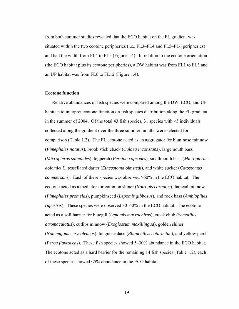
19
from both summer studies revealed that the ECO habitat on the FL gradient was
situated within the two ecotone peripheries (i.e., FL3–FL4 and FL5–FL6 peripheries)
and had the width from FL4 to FL5 (Figure 1.4). In relation to the ecotone orientation
(the ECO habitat plus its ecotone peripheries), a DW habitat was from FL1 to FL3 and
an UP habitat was from FL6 to FL12 (Figure 1.4).
Ecotone function
Relative abundances of fish species were compared among the DW, ECO, and UP
habitats to interpret ecotone function on fish species distribution along the FL gradient
in the summer of 2004. Of the total 43 fish species, 31 species with ≥5 individuals
collected along the gradient over the three summer months were selected for
comparison (Table 1.2). The FL ecotone acted as an aggregator for bluntnose minnow
(Pimephales notatus), brook stickleback (Culaea inconstans), largemouth bass
(Micropterus salmoides), logperch (Percina caprodes), smallmouth bass (Micropterus
dolomieui), tessellated darter (Etheostoma olmstedi), and white sucker (Catostomus
commersoni). Each of these species was observed >60% in the ECO habitat. The
ecotone acted as a mediator for common shiner (Notropis cornutus), fathead minnow
(Pimephales promelas), pumpkinseed (Lepomis gibbosus), and rock bass (Ambloplites
rupestris). These species were observed 30–60% in the ECO habitat. The ecotone
acted as a soft barrier for bluegill (Lepomis macrochirus), creek chub (Semotilus
atromaculatus), cutlips minnow (Exoglossum maxillingua), golden shiner
(Notemigonus crysoleucas), longnose dace (Rhinichthys cataractae), and yellow perch
(Perca flavescens). These fish species showed 5–30% abundance in the ECO habitat.
The ecotone acted as a hard barrier for the remaining 14 fish species (Table 1.2), each
of these species showed <5% abundance in the ECO habitat.

20
Table 1.2. Relative abundance comparison of each fish species among the downstream (DW, FL1–FL3), ecotonal (ECO, FL4–FL5), and upstream (UP, FL6–FL12) habitats on the Floodwood gradient over the summer months of 2004 (June– August).
DW ECO %UP
Alewife (Alosa pseudoharengus ) 100 0 0 7Black crappie (Pomoxis nigromaculatus ) 100 0 0 13Blacknose dace (Rhinichthys atratulus ) 0 2 98 885Blacknose shiner (Notropis heterolepis ) 100 0 0 7Bluegill (Lepomis macrochirus ) 78 22 0 521Bluntnose minnow (Pimephales notatus ) 6 69 25 466Bowfin (Amia calva ) 95 0 5 10Brook stickleback (Culaea inconstans ) 0 96 4 15Brown bullhead (Ictalurus nebulosus ) 89 0 11 74Comely shiner (Notropis amoenus ) 100 0 0 13Common carp (Cyprinus carpio ) 100 0 0 25Common shiner (Notropis cornutus ) 6 53 41 315Creek chub (Semotilus atromaculatus ) 0 11 89 473Cutlips minnow (Exoglossum maxillingua ) 0 20 80 1,736Fantail darter (Etheostoma flabellare ) 0 2 98 826Fathead minnow (Pimephales promelas ) 0 39 61 45Golden shiner (Notemigonus crysoleucas ) 83 17 0 41Largemouth bass (Micropterus salmoides ) 26 74 0 334Logperch (Percina caprodes ) 9 91 0 74Longnose dace (Rhinichthys cataractae ) 0 9 91 2,000Northern pike (Esox lucius ) 100 0 0 10Pumpkinseed (Lepomis gibbosus ) 65 35 0 531Redside dace (Clinostomus elongatus ) 0 0 100 19Rock bass (Ambloplites rupestris ) 12 58 30 313Sand shiner (Notropis stramuneus ) 0 0 100 28Smallmouth bass (Micropterus dolomieui ) 18 82 0 16Spottail shiner (Notropis hudsonius ) 100 0 0 13Stonecat (Noturus flavus ) 7 0 93 32Tessellated darter (Etheostoma olmstedi ) 4 90 6 307White sucker (Catostomus commersoni ) 0 82 18 1,884Yellow perch (Perca flavescens ) 77 23 0 255
Fish species Abundance (%) by habitat Total individuals1
1Cumulative individuals of each fish species collected along the gradient over the three summer months.

21
DISCUSSION
The peak turnover rates in fish species compositions indicated the ecotone
peripheries between ST6 and ST7 on the ST gradient and between FL5 and FL6 on the
FL gradient over the three summer months of 2002. However, using the abrupt
changes in habitat variables as the ecotone indicator yielded different results between
the two gradients. The congruence of the abrupt changes in habitat conditions and fish
species composition at the ecotone periphery on the ST gradient revealed a strong fish-
habitat relationship (e.g., Przybylski et al. 1991, Winemiller and Leslie 1992,
Rakocinski et al. 1992, Wagner 1999, Willis and Magnuson 2000, Gido et al. 2002,
Martino and Able 2003) across lentic-lotic transitions on the gradient. This
consequence conformed to the hypothesis that the ecotone formation could be detected
using abrupt changes in either habitat conditions or fish species composition. In
contrast, the similar pattern of coincidental abrupt changes in both fish species
composition and the habitat conditions was not detected on the FL gradient. While the
peak turnover rate in fish species composition was detected at the same location, the
changes in most of the habitat variables varied along the FL gradient.
Using habitat condition to detect ecotone formation is difficult when the changes
in the habitat variables are gradual (Hansen et al. 1988). In the summer of 2002,
average intensities of many habitat variables showed gradual or no changes at the FL
ecotone periphery. The complex mix of gradual and abrupt changes in habitat
conditions along the FL gradient diminished the efficiency of this indicator to define
ecotone location. From this result, the peak turnover rate in fish species composition
appears to be the most powerful indicator for depicting the FL ecotone. This is based
on the ideas that changes in species assemblages across a transition zone can

22
apparently reflect both gradual and abrupt changes in habitat conditions (Armand
1992, Strayer et al. 2003, Hoeinghaus et al. 2004).
This study revealed that there were no shifts in ecotone location over the summer
periods. The ecotone peripheries (that indicated the ecotone orientation between lentic
and lotic systems) on both gradients were static in their locations throughout each
study summer period. The fix in location of the ecotones may be due to
environmental discontinuities (Pinay et al. 1990, Delcourt and Delcourt 1992). In this
study, unidirectional water flow from upstream towards downstream on the gradients
promotes mixing of materials and results in spatiotemporal heterogeneities and
physical discontinuities (Ward and Stanford 1983, Pinay et al. 1990) at the particular
gradient portions. The strong physical discontinuities (e.g., abrupt changes in water
depth, current velocity, substrate composition, and stream geomorphology) can
contribute to the stable formation of ecotones over space and time (Pinay et al. 1990).
Previous studies on similar gradient patterns by Przybylski et al. (1991) and Willis
and Magnuson (2002) concluded that river mouths connecting with lakes appeared to
be the ecotones with the highest abundance and species richness of fish observed, and
these conformed to the edge effect (Odum 1971). However, no quantitative methods
were used to define the ecotone formation in those studies. For this study, the ecotone
formation on both gradients was defined using statistical methods. The orientations of
both ST and FL ecotones were detected between the downstream and midstream
stations where the transitional conditions between lentic and lotic systems occurred
instead of at the stations between Lake Ontario and the embayments. These findings
indicated that differences in the sizes of the study gradients, habitat conditions, or
geographical regions (Kolasa and Zalewski 1995) could also contribute to the different
formation patterns and characteristics of the aquatic ecotones.

23
Methods of collecting fish species assemblages are another factor that can
influence the determination of the ecotone locations on the lentic-lotic gradients.
From this study, the ecotone periphery on the ST gradient was detected at the location
where the sampling procedure was changed from boat to manual electrofishing.
However, the ecotone periphery on the FL gradient was detected at the location where
the same sampling procedure was used (i.e., manual electrofishing). Although the
change from boat to manual electrofishing between the deep and shallow stations was
unavoidable in this study, the same electricity output was generated for stunning fish
with a similar pace of locomotion in all stations, and thorough samplings were
conducted to cover all habitat types in each station. From these efforts, the method
constraint for collecting fish between the deep and shallower stations on the gradients
might only trivially affect the results. Additionally, Rakocinski et al. (1992) indicated
that differences in fish species assemblages along environmental gradients represent
species-specific differences in habitat use rather than gear bias.
Ecotone distinctiveness can be scale dependent (Johnston et al. 1992, Wiens 1992,
Fagan et al. 2003), thus a proper spatial sampling design is required to determine an
ecotone (ecotone peripheries plus ecotone width—ECO habitat). For example, an
ecotone that is very abrupt on a community scale may be too small to be detected on a
continental scale because the resolution of data collection (on the continental scale) is
too broad (Johnston et al. 1992, Fagan et al. 2003). Hence, the scale of data
observation must be commensurate with the scale of an ecotone in a study (Johnston et
al. 1992, Wiens 1992, Fortin et al. 2000, Csillag et al. 2001, Cadenasso et al. 2003).
Using the fish species turnover rate as the ecotone indicator, the results from the field
observations along the FL gradient in both summers of 2002 and 2004 confirmed that
the FL ecotone was static at the same location during the summer periods. With the
finer and proper scale of study in the second summer, the entire ecotone was

24
successfully determined, and it was situated within the ecotone periphery detected in
the summer of 2002 (Figure 1.4).
Conditions in habitats adjacent to an ecotone play a strong role in governing the
ecotone geometry and permeability (Stamps et al. 1987, Wiens 1992, Fortin 1994,
Fagan et al. 2003). In this study, the ECO habitat on the FL gradient represents a
mixed zone of transition between the lentic and lotic systems. Based on the ecotone
orientation, the lower portion of the ECO habitat is most likely to be influenced by the
transition between the embayment and downstream conditions at the lower ecotone
periphery (between FL3 and FL4, Figure 1.4: squares). Likewise, the upper portion of
the ECO habitat tended to be affected by the transition between downstream and
midstream conditions at the upper ecotone periphery (between FL5 and FL6, Figure
1.4: squares). Consequently, the ECO habitat appears to be a unique area providing
diverse permeability (Wiens et al. 1985, Wiens 1992, Cadenasso et al. 1997, Ross
2005) for the distribution of fish species assemblages on the gradient.
Of the four ecotone functions (i.e., aggregator, mediator, soft barrier, and hard
barrier) on fish species assemblages, the “edge effect” of an increase in fish abundance
and species richness (Odum 1971) was not observed at the FL ecotone. In contrast,
the ecotone acted as a hard barrier allowing very low permeability for most of the fish
species observed in the summer of 2004 (Table 1.2). The physical discontinuities in
space or patch contrast appear to be another important factor affecting the species
distribution (Pinay et al. 1990, Forman and Moore 1992, Wiens 1992, Wiens 2002).
From the field observations, small cascades and long runs existing above the upper
ecotone periphery possibly obstruct the distribution of some stream fish species into
the ecotone. In addition, the decrease of water depth observed at the lower ecotone
periphery acted as a hard obstacle for many fish species to migrate into the ecotone.
While the FL ecotone provided low-to-zero permeability for most fish species, it was

25
concurrently a nursery ground for seven species (i.e., bluntnose minnow, brook
stickleback, largemouth bass, logperch, smallmouth bass, tessellated darter, and white
sucker). These particular species aggregated (>60%) in the ECO habitat during the
study summer, and most of the individual fish by species were young (0+ year-old).
The fundamental knowledge about ecotone formations on the two embayment-stream
gradients and the ecotone functions on fish species assemblages are useful for better
understanding ecotone properties in aquatic systems and future applications in
resource management (e.g., Petts 1990, Sisk and Haddad 2002) and fish habitat
restoration (Kirchhofer 1995, Kolasa and Zalewski 1995).
Overall, the results from this study show that the turnover rate in fish species
composition appears to be the best ecotone indicator on the embayment-stream
gradients. While abrupt changes in habitat conditions and species composition may
coincidentally occur at the same location reflecting the strong fish-habitat
relationships, the habitat variables showed less efficiency in defining the ecotone
formation on the gradient with the complex mix of habitat conditions. An appropriate
scale of study is required to determine ecotone width. The distinct physical
discontinuities below and above the ecotone detected on the FL gradient contributed to
low permeability of the ecotone on flux of the fish species. This study is the first
effort of its type using both biotic and non-biotic variables to detect ecotone formation
in the freshwater system associated with Lake Ontario. To explore ecotone properties
in a different water system, both functions and formations of ecotones were detected
along the tidal Hudson River, one of the world’s largest marine-freshwater gradients.
The methodology of study, results, and discussion are presented in Chapter 2.

26
CHAPTER TWO
Ecotone properties in the Hudson River estuary, New York
ABSTRACT
Ecotone properties were determined on the Hudson River estuary gradient during
1974–2001. Turnover rate in fish species composition was used to detect ecotone
formations and abundances of fish species assemblages in and around ecotones were
used to interpret ecotone functions. From the results, the Hudson ecotones showed
both changes in location and structure spatially and temporally. In some time periods,
the ecotones changed in their breadth (from broader to narrower or vice versa) or
considerably declined to be just ecotone peripheries. The ecotone peripheries mostly
detected at the lower gradient portion might result from the sharp changes in dissolved
oxygen (DO) and water salinity within this gradient range. The ecotone peripheries
mostly detected at the upper gradient portion might result from the abrupt changes in
DO, water temperature, SAV abundance, and dam constructions within this gradient
range. The ecotones were highly detected at the lower-middle portion of the gradient
and their formations tended to relate with the changes in salinity, tide, and freshwater
flow. Functional patterns of the Hudson ecotones were not distinctly different over
time. One ecotone mostly detected in the lower-middle gradient portion appeared to
be the optimal zone for distributions of diverse fish assemblages. However, the other
detected ecotones acted as barriers for most fish species. Likewise, the ecotone
peripheries inhibited distributions of most fish species. These results might relate with
complex migratory behaviors and life histories of fish and their responses to variations
in the estuarine conditions in space and time.

27
INTRODUCTION
Ecotone studies have been prominent and appealing (e.g., Clements 1897, Leopold
1933, Odum 1971, Risser 1990, Winemiller and Leslie 1992, Lidicker 1999, Willis
and Magnuson 2000, Harding 2002, Martino and Able 2003, Ries et al. 2004) because
of the important roles of ecotones on biodiversity (di Castri and Hansen 1992, Neilson
et al. 1992, Lachavanne 1997), biotic interactions (Wiens et al. 1993), flows of
materials and nutrients in ecosystems (Hansen and di Castri 1992), and the ecological
implications for natural resources management at the individual, population, and
ecosystem levels (Sisk and Haddad 2002). Clements (1897) was the first who viewed
an ecotone as the transition zone between different plant communities. He observed
that the vegetation in this zone was often accentuated in size and density. Leopold
(1933) later explained that shape and spatial configuration of an ecotone influence
species richness and organism abundance. Working with these early ideas, Odum
(1971) defined an ecotone as a transition zone between two or more communities and
he labeled the increases in both species richness and abundance at the ecotone as a
result of the “edge effect”.
At present, an ecotone is widely viewed as a transition zone between adjacent
ecological systems and its influences on organism distributions have been considered
beyond the traditional edge effect. Additionally, scientists may use diverse terms to
call a transition zone depending on the spatial scale considered and the prior
delineation of the system of interest. In this study, an ecotone periphery is used to
represent a narrow transition zone or a boundary with one less dimension than a patch
(e.g., Stamps et al. 1987, Fagan et al. 1999, Strayer et al. 2003), whereas an ecotone
refers to a broader transition zone (Fagan et al. 1999) comprising ecotonal habitat and
ecotone peripheries. An ecotone may form, decline, disappear, shift locations, or
change in terms of structure (from an ecotone to be just an ecotone periphery) or

28
function due to the influence of changing physicochemical conditions, species use of
habitat, and interactions among species (Holland 1988, Delcourt and Delcourt 1992,
Wiens 1992, Kolasa and Zalewski 1995).
As a zone of transition in biotic and physicochemical conditions, an ecotone
provides different permeability on flux of organisms. In this study, ecotone
permeability is considered in terms of ecotone function on organism distributions.
Other than attracting particular organisms, the mechanism that produces the edge
effect may simultaneously inhibit dispersion of other organisms into an ecotone. The
same ecotone may be neutral and has no effect on distribution of some other species
into the ecotone. Dynamic properties (formation and function) of ecotones can be
obviously observed in an estuary, a complex ecosystem where the interaction between
marine and freshwater systems occur, and tide and water flow play strong influence.
As one of the world’s important estuaries, the tidal Hudson River drainage serves
more than 200 fish species (Stanne et al. 1996, Daniels et al. 2005) from freshwater,
estuarine, and marine assemblages. Other than providing variety of habitats for
aquatic creatures, the Hudson River estuary has been heavily altered by human
activities, such as urbanization, shoreline development, dam construction, power plant
operation, and water diversion for commercial, industrial, and agricultural purposes
(Limburg et al. 1986, Barnthouse et al. 1988, Schmidt and Cooper 1996, Wall and
Phillips 1998, Baker et al. 2001, Phillips et al. 2002, Daniels et al. 2005).
The tidal Hudson River portions where the intermediate conditions between fresh
and saline waters meet are apparently vital ecotones for living of various fish species,
especially in their first year of life (Weinstein et al. 1980, Stanne et al. 1996). At the
lower-middle portion of the tidal Hudson River, the locations and spatial structures of
the Hudson ecotones tend to vary in space and time due to the changes in salinity
regime, tide, and freshwater runoff. At the upper portions of the tidal Hudson River,

29
effects of dam constructions and water pollutions, e.g., low dissolve oxygen, high
coliform densities (Boyle 1979), and large loads of polychlorinated biphenyls
discharged from several general electric factories above the Federal Dam (Baker et al.
2001) may contribute to sharp formations of ecotone peripheries affecting fish
distributions below and above the Federal Dam. Although ecotone formations and
their functions on organism distributions can be used as a baseline for resources
managers to maximize healthy habitats for species assemblages of interest, these
ecotone properties have never been revealed in the Hudson system.
The first objective of this study was to detect ecotone formations on the Hudson
River estuary gradient. Spatial structures of the Hudson ecotones were determined
under the hypothesis that complex mix of abrupt and gradual changes in habitat
conditions might contribute to the formation of an ecotone (comprising ecotonal
habitat and ecotone peripheries), whereas abrupt changes in habitat conditions might
contribute to a narrow formation of an ecotone periphery alone. Over space and time,
some ecotones may be fixed in location, new ecotones may form, or former ecotones
may decline or change in their breadths. The study habitat variables were dissolved
oxygen, salinity, water temperature, two major types of submerged aquatic vegetation
(Trapa natans and Vallisneria americana), and bottom substrates of water. Changing
patterns of these habitat variables in and around the ecotone pay strong role on
distribution patterns of fish assemblages along the Hudson River estuary gradient.
The second objective of the study was to detect ecotone functions on the Hudson
fish species assemblages over time. Ecotone functions on fish species assemblages are
interpreted from observed abundance of fish by species in and around an ecotone. An
ecotone may act as an aggregator for particular fish species. Concurrently, it may act
as a hard barrier completely blocking distribution of some fish species into the
ecotone, or as a soft barrier partially allowing some fish species to enter the ecotone.

30
In the latter case, most species populations entering the ecotone will return to the
habitats from which they came, causing few of them to be observed in the ecotone.
An ecotone formed somewhere on the Hudson River estuary gradient may act as a
mediator for marine and freshwater fish species with broad tolerance on changing
salinity. Over space and time, an ecotone may decline in its structure to be just an
ecotone periphery and may completely or partly inhibit distribution of particular fish
species between adjacent habitats. Concomitantly, an ecotone periphery may be
neutral and has no effect on fish distributions between adjacent habitats it separates.
MATERIALS AND METHODS
Study gradient and data sources
The Hudson River estuary starts from Battery at river kilometer (RKM) 1 in
Manhattan, New York City, to the Federal Dam at RKM 246 in Troy, Albany, New
York State (Figure 2.1). In this study, the gradient was divided into four zones. The
lowest zone (RKMs 1–19) was normally polyhaline with salinity concentration of 18–
30 ppt (Ristich et al. 1977, National Oceanic and Atmospheric Administration 1989).
At this zone, the river channel was approximately 1 km wide and 9–15 m deep (Coch
and Bokuniewicz 1986). The above three zones (the lower, the middle, and the upper
zones) were classified following Schmidt et al. (1988).
31
Figure 2.1. The Hudson River estuary gradient showing 13 regions designated for the five power plant utilities’ Hudson River estuary monitoring program.

32
At the lower zone (RKMs 19–61), the river channel was 1.0–1.5 km wide and 13–
17 m deep (Coch and Bokuniewicz 1986). At the middle zone (RKMs 61–122), the
river channel was 0.5–1.0 km wide and 18–48 m deep (Coch and Bokuniewicz 1986).
At the upper zone (RKMs 122–246), the river channel was 0.6–1.2 km wide and 15–
31 km deep (Coch and Bokuniewicz 1986). Salinity in water varies temporally
between mesohaline and oligohaline in the lower and the middle zones depending on
tide and freshwater flow, while water was usually fresh in the upper zone (Strayer et
al. 2004).
Fish data used to determine ecotone properties on the Hudson River estuary
gradient were from the beach seine survey (BSS) during 1974–2001 of the Utilities’
Hudson River estuary monitoring program. The Utilities collectively represents the
five power plant utilities including Central Hudson Gas and Electric Corporation,
Consolidated Edison Company of New York Inc, New York Power Authority, Niagara
Mohawk Power Corporation, and Southern Energy New York. Based on the
monitoring program, the Hudson River estuary was divided into 13 regions (RE)
starting from RE0 (RKMs 1–19) to RE12 (RKMs 201–246; Figure 2.1).
The monitoring program used stratified random samplings to conduct the BSS
along the tidal river gradient. According to the stratification method, fish assemblages
were randomly sampled along the shore zone (≤3-m water depth) using a 30.5-m total
length beach seine with a 0.5-cm bag mesh size. At each sampling point, one end of
the net (of the beach seine) was held on shore and the other end was towed
perpendicularly away from shore by boat sweeping approximately 450 m2 of sampling
area. Main purpose of the survey was to obtain abundance and distribution data of
young of the year of target fish species including Atlantic tomcod (Microgadus
tomcod), American shad (Alosa sapidissima), striped bass (Morone saxatilis), and

33
white perch (Morone americana) along inshore zone of the Hudson River estuary
(Texas Instruments 1981).
At least three observations were taken at each region in each sampling period of
the BSS. Yearly numbers of the observations were 2,331–3,648 during 1974–1980,
500–800 during 1981–1984, and 1,000 during 1985–2001. The BSS was done weekly
from: April to the 2nd week of December during 1974–1975 and 1978–1979, April
through November during 1976–1977, April to the 3rd week of August and then
biweekly through November in 1980. During 1981–1995, the BSS was done biweekly
each year. The biweekly survey schedules were from: August to the 2nd week of
October during 1981–1983, last week of July to the 1st week of October in 1984, the
2nd week of July to the 3rd week of November during 1985–1986, the 4th week of June
to the 2nd week of November in 1987, June through October during 1988–1992 and
1994–1995, and last week of June to the 1st week of November 1993. During 1996–
2001, the BSS was done biweekly each year from July to the 3rd week of October.
The BSS method in detail can be found from the Utilities’ early or recent monitoring
programs (e.g., Texas Instruments 1977, ASA Analysis & Communication 2004).
Habitat data including dissolved oxygen (DO), salinity, water temperature,
submerged aquatic vegetation (SAV), and substrate composition were used to describe
habitat conditions along the Hudson River estuary gradient (RE1–RE12) in this study.
The first three habitat variables were from the Utilities’ BSS, and they were in-situ
measured at approximately 0.3 m below the water surface and 15 m from the shoreline
using a YSI Model 57 Dissolved Oxygen Meter (Texas Instruments 1976). Mean
value for each of the three habitat variables at each sampling location and sampling
week, weighted by stratum volume, was calculated using equation (1) as

34
∑=
=rwn
iirwrwrw n
1W/1W , (1)
where Wrw is the mean of a habitat variable at river mile r during bi-week w of the
BSS, Wirw is a habitat measurement for location i at river mile r during bi-week w, and
nrw is a number of habitat measurement taken at river mile r during bi-week w. DO
was measured to the closet 0.1 mg/L, and water temperature was measured to the
closest 0.1°C. Conductivity of water was measured in millisieman/cm at 25 °C (C25)
and it was used to compute salinity concentration (ppt) using equation (2) as (Texas
Instruments 1976)
Salinity = -100 ln (1-C25/178.5) (2)
SAV data were from the study by the collaboration among the Institute of
Ecosystem Studies, the Hudson River National Estuarine Research, New York State
Department of Environmental Conservation (NYSDEC), and the Cornell Institute for
Resource Information Systems. The SAV study was conducted from RE2 to RE12 in
August 1995 and July–August 1997. Photographic, digital, and grab sampling data
were used to classify and map bed areas of Trapa natans (water chestnut—rooted with
floating leaves) and Vallisneria americana (water celery).
Substrate data from the Utilities’BSS (1974–2001) and NYSDEC (1998–2003)
were combined to describe bottom condition along the study gradient. The Utilities’
substrate data were observed in shallow water areas (≤3 m deep) from RE1 to RE12
and its composition was classified into four types: mud, sand, gravel with <76 mm
grain size, and gravel with ≥76 mm grain size. The NYSDEC’s substrate data were
collected across the Hudson River estuary system, but they were not completely done

35
in shallow water <4 m deep (Bell et al. 2006). Both core and grab samples were
categorized with some guidance from the acoustic backscatter data (Nitsche et al.
2004) and the sediment profiler imagery data (Rhoads and Cande 1971, Rhoads and
Germano 1982). Based on grain size and percentage composition, the NYSDEC’s
substrates were classified into: mud (<0.062 mm grain size), sand (0.062–2 mm),
gravel (2–36 mm), and six mixed groups including sandy mud (mud with >10% sand),
gravelly mud (mud with >10% gravel), muddy sand (sand with >10% mud), gravelly
sand (sand with >10% gravel), muddy gravel (gravel with >10% mud), and sandy
gravel (gravel with >10% sand).
Ecotone and habitat analyses
Because the Utilities’ BSS was not conducted in RE0 prior to 1996, the ecotone
and habitat analyses were done from RE1 to RE12 on the tidal Hudson River gradient
based on the BSS fish and habitat data available from 1974 to 2001. Ecotone
formation was detected monthly in all years the fish data were available for all 12
regions (RE1–RE12). Turnover rate or beta diversity (Whittaker 1975, Gauch 1982,
Delcourt and Delcourt 1992, Winemiller and Leslie 1992, Wagner 1999, Hoeinghaus
et al. 2004) in fish species composition was used to detect ecotone formation on the
gradient. Detrended correspondence analysis (DCA) in CANOCO 4.0 software (ter
Braak and Smilauer 1998) was used to compute the beta diversity (hereafter called
beta A) based on both occurrence and percentage abundance by species of fish in each
region. In the computation, the sample scores on the DCA ordination are rescaled into
the average standard deviation (SD) units of species turnover (Hill 1979). A gradient
length of 1.0 SD represents approximately one-fourth of a complete turnover rate in
species composition on the gradient (Gauch 1982). Species appear, rise to their
modes, and disappear over a distance of about 4 SD. That is, if the beta A on the

36
DCA’s axis 1 (that accounts for the most variation) is ≥4.0 SD, it indicates that species
compositions at both extreme ends of a gradient represent completely different
communities (Gauch 1982). This indicates complete formation of at least one ecotone
on the gradient. The peak absolute difference (≥1 SD for this study) in the beta A (δ
beta A) indicates an ecotone periphery (a margin where a sharp transition between
adjacent habitats occurs).
Multiple functions of an ecotone (an ecotonal habitat plus its ecotone peripheries)
were interpreted from the relative observed abundance by species of fish among an
ecotonal habitat, an upper adjacent habitat, and a lower adjacent habitat. This study
proposed that an ecotone acts as an aggregator for a fish species with >60% abundance
observed in the ecotonal habitat and as a mediator for fish species with 30–60%
abundance observed in the ecotonal habitat. Concurrently, an ecotone acts as a soft
barrier for a fish species with 5–30% abundance observed in the ecotonal habitat.
Lastly, an ecotone acts as a hard barrier for a fish species with <5% abundance
observed in the transitional habitat. Forming as an ecotone periphery (ep) between
adjacent habitats (without ecotone width), the ep may be neutral allowing fish species
with >30% abundance to distribute between the adjacent habitats. Concurrently, an ep
may partly or completely inhibit distribution of a fish species from one habitat to the
other adjacent habitat causing low (5–30%) or lower-absent (0–5%) abundance,
respectively, of fish in the latter habitat. Each fish species with <5 individuals
observed along the gradient in each analyzed time period (i.e., a certain month in a
certain year) was not included in the comparison because of low catch.
General linear model with multivariate analysis of variance (GLM MANOVA)
procedure in SPSS version 14.0 software was used to compare mean values of DO,
salinity, water temperature, and their associated delta values (i.e., absolute difference
between minimum and maximum values) between two periods of ecotone analysis

37
(i.e., non-detected period, ECO = 0 and detected period, ECO = 1) and due to the
interactions of ECO × RE, ECO × Month, ECO × Year, ECO × RE × Month, ECO ×
RE × Year, and ECO × Month × Year. Tukey’s honestly significant differences
(HSD) test was used to monthly compare mean values of each habitat variable
between paired regions when the significant difference of the variable was detected.
Bed areas (km2) of two SAV species (Trapa natans and Vallisneria americana) from
the SAV shapefile were estimated by region along the Hudson River estuary gradient
using ArcGIS 9.1.
Area (km2) of each substrate type including mud (<0.062 mm grain size), sand
(0.062–2 mm), gravel (2–76 mm), cobble (>76 mm), and the six mixed groups from
the NYSDEC and Utilities’ datasets were combined and re-calculated. Because the
NYSDEC’s substrate data were less completed along the Hudson inshore zone, only
offshore area for each substrate type was retrieved from this dataset and summed up
with the inshore area of the associated substrate type estimated from the Utilities’ BSS
for each associated region. That is, after the area for each substrate type from the
NYSDEC’s shapfile was estimated by region using ArcGIS 9.1, the offshore area for
each substrate type in each associated region was re-computed using equation (3) as
follows:
( )Utilities(shore,DEC)(total,DEC)(total,
DEC),(sub,offshore)(sub AreaArea
Area
AreaArea ii
i
jiji −×= , (3)
where Areai(sub j, offshore) is the estimated area of substrate type j at region i (i = 1, 2,
3,…, 12) in the offshore zone, Areai(sub j, DEC) is the estimated area of substrate type j at
region i based on the NYSDEC’s data, Areai(total, DEC) is the estimated area for all
substrate types at region i based on the NYSDEC’s data, and Areai(shore, Utilities) is the
estimated area in the inshore zone at region i based on the Utilities’ data.

38
RESULTS
A total of 127 fish species (excluded 14 unidentified species) from 47 families was
recorded along the Hudson River estuary gradient (RE1–RE12) from the BSS during
1974–2001. Of the 47 families, four families: Cyprinidae, Centrarchidae, Clupeidae,
and Sciaenidae had the highest species richness. Blueback herring (Alosa aestivalis)
was the most abundant (34%) species and distributed throughout the Hudson River
estuary. The latter four fish species with >8% observed abundance on the gradient
were bay anchovy (Anchoa mitchilli, 9%), white perch (Morone americana, 9%),
unidentified clupeid (9%), and American shad (Alosa sapidissima, 8%).
Distribution patterns of fish along the Hudson River estuary gradient are
apparently shaped by fish migratory behaviors (anadromous and catadromous) and
salinity tolerance across marine-estuarine and estuarine-freshwater transitions. Based
on these criteria, the Hudson fish species were classified into five assemblages,
comprising anadromous, catadromous, estuarine, freshwater, and marine (Smith
1985). Of the total 127 identifiable fish species recorded along the gradient, nine
species were anadromous fish, one species (American eel—Auguilla rostrata) was
catadromus, 13 species were estuarine fish, 59 species were freshwater fish, and 45
species were marine fish (Appendix 2.1).
Ecotone formation and function
The ecotones were detected in 116 time periods (76%) of the total 152 time
periods the fish data were available for the analysis during 1974–2001 (Figure 2.2).

39
Figure 2.2. Frequency of ecotones detected monthly based on the data collection along the Hudson River estuary gradient during 1974–2001.

40
The ecotone was detected with the highest frequency (18 times) at RE2, while the
ecotone peripheries alone were highly detected between RE1 and RE2 (18 times) and
between RE11 and RE12 (30 times) on the Hudson River estuary gradient (Figure
2.3). Ecotones and ecotone peripheries were less detected at the remaining portions on
the gradient (Figure 2.3).
Figure 2.3. Ecotones (thick bars) and ecotone peripheries (thick lines) detected during 1974–2001on the Hudson River estuary gradient covering 228 river kilometers (RKM) from region (RE) 1 to RE12 are grouped into each frequency class. Numbers of times of the formation of an ecotone and an ecotone periphery in each location are shown in brackets in each frequency class on the right side of the graph.
With the highest frequency (18 time periods) of detection at RE2, this ecotone
acted as a hard barrier for most (>35%) of the total fish species observed along the

41
gradient in the associated time periods (Table 2.1). Similarly, the ecotones detected at
other locations (except at RE2–RE4) acted as a hard barrier for most of the Hudson
fish species (Table 2.1, see ecotone functions from all detected frequencies in
Appendix 2.2). Detecting 10 times at RE2–RE4, this ecotone acted as an aggregator
for most of the fish species observed from the six time periods (July 1986, August
1979, September 1982 and 1988, October 1975, and November 1986), but it acted as a
mediator, soft barrier, or hard barrier for most of the fish species observed in the rest
time periods (Table 2.1). Consistent with most of the ecotones functioning as hard
barriers, the ecotone peripheries detected alone between particular adjacent regions on
the gradient completely inhibited the distribution between the adjacent regions of most
(>35%) fish species in the analyzed time periods (Table 2.2, see ecotone periphery
functions from detected frequencies in Appendix 2.3).
Table 2.1. Functions of the ecotones detected ≥5 times at certain regions (RE) and time periods on Hudson fish species assemblages.
Ecotone No. of selected1
location Aggregator Mediator Soft barrier Hard barrier species/gradient
RE2May-75 3.1 21.9 28.1 46.9 32May-76 6.7 26.7 26.7 39.9 30May-78 15.6 12.5 21.9 50.0 32Jun-74 8.8 11.8 20.6 58.8 34Jun-75 10.9 16.2 24.3 48.6 37Jun-76 12.2 9.8 34.1 43.9 41Jun-77 16.7 13.9 25.0 44.4 37Jul-78 7.0 18.6 14.0 60.4 43Jul-79 26.2 28.6 11.9 33.3 42Jul-84 31.0 21.4 9.5 38.1 42Jul-90 32.3 19.4 12.9 35.4 31Aug-78 10.2 18.4 20.4 51.0 49Aug-84 36.6 14.6 22.0 26.8 41Aug-96 21.4 10.7 17.9 50.0 28Sep-84 31.3 12.5 15.6 40.6 32Nov-76 18.2 13.6 22.7 45.5 22Nov-79 37.5 17.5 12.5 32.5 40Dec-78 0.0 11.1 27.8 61.1 18
Function (%) for the total selected species

42
Table 2.1 (Continued).
Ecotone No. of selected1
location Aggregator Mediator Soft barrier Hard barrier species/gradient
RE2-RE3Jun-91 19.0 23.9 21.4 35.7 42Jul-00 20.0 17.1 8.6 54.3 35Sep-79 42.9 34.3 11.4 11.4 35Sep-81 27.9 9.3 23.3 39.5 43Sep-87 46.0 16.2 18.9 18.9 37Sep-99 12.5 6.3 18.8 62.4 32Oct-83 36.8 5.3 21.1 36.8 19Nov-78 16.7 33.3 13.3 36.7 30
RE2-RE4Jul-86 42.1 15.8 18.4 23.7 38Aug-74 22.0 30.0 22.0 26.0 50Aug-79 36.4 25.0 18.1 20.5 44Sep-82 38.5 25.6 18.0 17.9 39Sep-88 51.5 9.1 15.2 24.2 33Sep-96 30.0 20.0 30.0 20.0 20Oct-75 38.9 22.2 22.2 16.7 36Oct-98 22.6 19.4 6.5 51.5 31Nov-80 23.5 29.5 23.5 23.5 17Nov-86 36.0 28.0 12.0 24.0 25
RE3-RE4Apr-74 50.0 11.1 16.7 22.2 18May-78 37.5 37.5 15.6 9.4 32Jun-75 29.8 40.5 10.8 18.9 37Jul-75 25.6 30.2 23.3 20.9 43Aug-81 18.0 35.9 28.2 17.9 39Aug-97 3.6 25.0 42.8 28.6 28Sep-01 3.5 13.8 24.1 58.6 29Oct-84 20.1 23.3 33.3 23.3 30Dec-78 38.9 27.8 11.1 22.2 18
RE3-RE5Aug-98 15.2 18.2 33.3 33.3 33Sep-98 7.0 10.3 37.9 44.8 29Oct-85 20.0 20.0 50.0 10.0 30Oct-92 21.4 25.0 14.3 39.3 28Nov-87 14.3 7.1 35.7 42.9 14
RE4-RE5Jul-90 3.2 9.7 12.9 74.2 31Aug-99 8.2 10.8 32.4 48.6 37Oct-83 15.8 26.3 31.6 26.3 19Oct-93 13.3 20.1 33.3 33.3 30Sep-81 4.7 9.3 44.2 41.8 43
RE5Jun-91 0.0 4.8 26.2 69.0 42Jun-92 0.0 8.3 25.0 66.7 24Jul-93 0.0 13.9 22.2 63.9 36
Function (%) for the total selected species
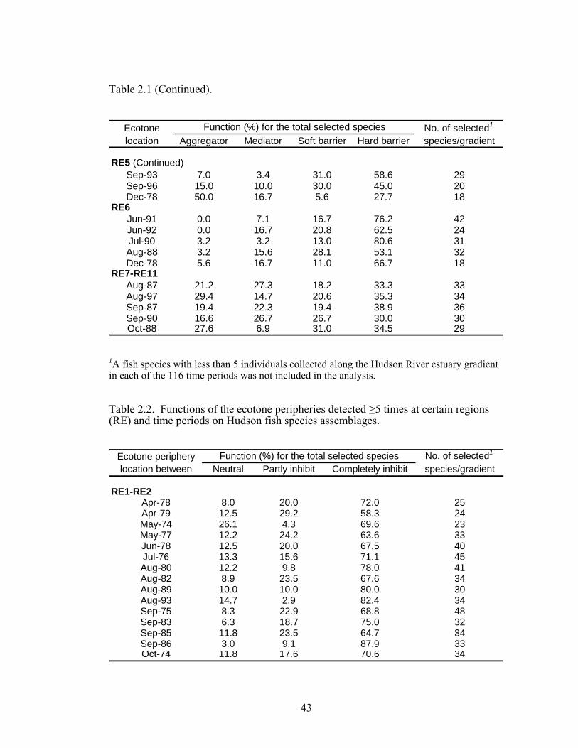
43
Table 2.1 (Continued).
Ecotone No. of selected1
location Aggregator Mediator Soft barrier Hard barrier species/gradient
RE5 (Continued)Sep-93 7.0 3.4 31.0 58.6 29Sep-96 15.0 10.0 30.0 45.0 20Dec-78 50.0 16.7 5.6 27.7 18
RE6Jun-91 0.0 7.1 16.7 76.2 42Jun-92 0.0 16.7 20.8 62.5 24Jul-90 3.2 3.2 13.0 80.6 31Aug-88 3.2 15.6 28.1 53.1 32Dec-78 5.6 16.7 11.0 66.7 18
RE7-RE11Aug-87 21.2 27.3 18.2 33.3 33Aug-97 29.4 14.7 20.6 35.3 34Sep-87 19.4 22.3 19.4 38.9 36Sep-90 16.6 26.7 26.7 30.0 30Oct-88 27.6 6.9 31.0 34.5 29
Function (%) for the total selected species
1A fish species with less than 5 individuals collected along the Hudson River estuary gradient in each of the 116 time periods was not included in the analysis.
Table 2.2. Functions of the ecotone peripheries detected ≥5 times at certain regions (RE) and time periods on Hudson fish species assemblages.
Ecotone periphery No. of selected1
location between Neutral Partly inhibit Completely inhibit species/gradient
RE1-RE2Apr-78 8.0 20.0 72.0 25Apr-79 12.5 29.2 58.3 24May-74 26.1 4.3 69.6 23May-77 12.2 24.2 63.6 33Jun-78 12.5 20.0 67.5 40Jul-76 13.3 15.6 71.1 45Aug-80 12.2 9.8 78.0 41Aug-82 8.9 23.5 67.6 34Aug-89 10.0 10.0 80.0 30Aug-93 14.7 2.9 82.4 34Sep-75 8.3 22.9 68.8 48Sep-83 6.3 18.7 75.0 32Sep-85 11.8 23.5 64.7 34Sep-86 3.0 9.1 87.9 33Oct-74 11.8 17.6 70.6 34
Function (%) for the total selected species

44
Table 2.2 (Continued).
Ecotone periphery No. of selected1
location between Neutral Partly inhibit Completely inhibit species/gradient
RE1-RE2 (Continued)Oct-77 15.2 27.3 57.5 33Oct-81 16.7 13.9 69.4 36Nov-77 14.7 23.5 61.8 34
RE3-RE4Jun-88 17.1 17.1 65.8 35Jul-96 18.0 25.6 56.4 39Sep-76 18.0 41.0 41.0 36Sep-80 11.1 33.3 55.6 36Sep-94 8.6 17.1 74.3 35Oct-78 25.7 34.3 40.0 35Oct-80 15.4 26.9 57.7 26Oct-86 25.8 29.0 45.2 31Oct-95 13.3 30.0 56.7 30
RE10-RE11Jun-74 35.3 35.3 29.4 34Jun-78 22.5 35.0 42.5 40Jul-75 30.2 30.2 39.6 43Aug-79 29.5 29.5 41.0 44Sep-75 22.9 14.6 62.5 48Sep-80 30.6 19.4 50.0 36Oct-74 14.7 38.2 47.1 34Nov-80 11.8 5.9 82.3 17Nov-86 24.0 24.0 52.0 25
RE11-RE12May-74 13.1 21.7 65.2 23May-77 9.1 30.3 60.6 33May-78 21.9 18.7 59.4 32May-80 16.7 13.9 69.4 36Jun-79 13.9 16.7 69.4 36Jun-80 20.0 32.5 47.5 40Jun-95 9.6 33.3 57.1 21Jul-76 19.5 31.7 48.8 41Jul-77 14.0 25.5 60.5 43Jul-78 28.6 26.2 45.2 42Jul-97 8.6 20.0 71.4 35Jul-00 20.6 32.4 47.0 34Aug-75 20.0 28.9 51.1 45Aug-76 29.2 20.8 50.0 48Aug-78 28.6 22.4 49.0 49Aug-80 26.8 19.5 53.7 41Sep-76 25.6 18.0 56.4 39Sep-78 28.9 15.8 55.3 38Sep-79 22.9 22.9 54.2 35Sep-82 20.5 18.0 61.5 39Sep-94 20.0 20.0 60.0 35Sep-99 18.8 43.8 37.4 32
Function (%) for the total selected species

45
Table 2.2 (Continued).
Ecotone periphery No. of selected1
location between Neutral Partly inhibit Completely inhibit species/gradient
RE11-RE12 (Continued)Sep-01 16.7 13.3 70.0 30Oct-76 10.3 25.6 64.1 39Oct-78 20.0 11.4 68.6 35Oct-79 22.3 19.4 58.3 36Oct-80 15.4 26.9 57.7 26Oct-93 10.3 13.8 75.9 29Nov-78 16.7 10.0 73.3 30Nov-79 13.4 23.3 63.3 30
Function (%) for the total selected species
1A fish species with less than 5 individuals collected along the Hudson River estuary gradient in each of the 116 time periods was not included in the analysis
Changing habitat related to ecotone formation
Only mean values of DO were significantly different (GLM MANOVA: p≤0.050)
between the non-detected (ECO = 0) and detected (ECO = 1) ecotone periods, whereas
mean values of DO, delta salinity, and delta water temperature were significantly
differences due to the interactions of ECO × RE (Table 2.3). Mean values of all
habitat variables and their associated deltas showed significant differences due to the
interactions of ECO × Month, ECO × Year, ECO × RE × Month, ECO × RE × Year,
and ECO × Month × Year (Table 2.3). Mean values of DO, salinity, and water
temperature were then further examined over space (RE) and time (Month) based on
the results from Turkey’s HSD post hoc.
The DO along the Hudson River estuary gradient ranged from 11 to 13 mg/L in
April, but decreased to 9–11 mg/L in May, and 7–10 mg/L during June–September.
The DO increased again to 8–10 mg/L in October and 10–14 mg/L in December
(Figure 2.4).

46
Table 2.3. Results from multivariate analysis of variance for each habitat variable and its delta (absolute difference between minimum and maximum values) between non-detected (ECO = 0) and detected (ECO = 1) ecotone periods and due to the interactions of ECO × RE (river region), ECO × Month, ECO × Year, ECO × RE × Month, ECO × RE × Year, and ECO × Month × Year.
Dependent Mean Variable Square
Dissolved oxygen 1 2.45 4.71 0.030Delta dissolved oxygen 1 0.02 0.01 0.921Salinity 1 0.03 0.06 0.804Delta salinity 1 1.27 1.03 0.311Water temperature 1 0.07 0.12 0.730Delta water temperature 1 2.01 0.60 0.440
Dissolved oxygen 11 1.08 2.07 0.020Delta dissolved oxygen 11 2.70 1.13 0.336Salinity 11 0.75 1.72 0.064Delta salinity 11 3.60 2.90 0.001Water temperature 11 0.97 1.78 0.053Delta water temperature 11 9.41 2.78 0.001
Dissolved oxygen 6 3.06 5.89 0.000Delta dissolved oxygen 6 8.59 3.59 0.002Salinity 6 3.59 8.21 0.000Delta salinity 6 8.95 7.23 0.000Water temperature 6 11.90 21.83 0.000Delta water temperature 6 23.04 6.81 0.000
Dissolved oxygen 18 3.53 6.79 0.000Delta dissolved oxygen 18 12.97 5.42 0.000Salinity 18 3.63 8.30 0.000Delta salinity 18 5.81 4.69 0.000Water temperature 18 9.73 17.86 0.000Delta water temperature 18 30.19 8.93 0.000
Dissolved oxygen 154 1.51 2.90 0.000Delta dissolved oxygen 154 2.94 1.23 0.043Salinity 154 2.11 4.84 0.000Delta salinity 154 2.88 2.33 0.000Water temperature 154 2.59 4.75 0.000Delta water temperature 154 7.37 2.18 0.000
Dissolved oxygen 493 1.27 2.44 0.000Delta dissolved oxygen 493 3.55 1.48 0.000Salinity 493 1.77 4.04 0.000Delta salinity 493 2.86 2.31 0.000Water temperature 493 0.63 1.16 0.026Delta water temperature 493 6.99 2.07 0.000
ECO × RE × Month
Source p-value
ECO × RE × Year
ECO
ECO × RE
ECO × Month
ECO × Year
df F

47
Mean values of DO between the detected and non-detected ecotone periods were
significantly different at particular region(s) in all eight months included in the
analysis, however, inconsistent patterns were shown over time (Figure 2.4).
Figure 2.4. Monthly mean values of dissolved oxygen observed along the Hudson River estuary gradient in the detected ecotone (line with solid dot markers) and non-detected ecotone (line with open dot markers) periods.

48
Focusing on mean values of DO in the detected ecotone period, the abrupt changes
of DO from RE1 to RE4 and between RE11 and RE12 in most of the analyzed months
(Figure 2.4) were parallel with high frequencies of detecting ecotones and ecotone
peripheries within this gradient range.
Unlike DO, the salinity showed consistent patterns of change over time along the
Hudson River estuary gradient. Mean values of salinity along the gradient were lower
in April and May, but higher in June, October, and December, and reached the highest
during July–September (Figure 2.5). In general, the salinity was the highest at RE 1
that was influenced by the marine conditions of New York Bay and it abruptly
decreased over distance until became tidal fresh at the upper zone of the gradient
(Figure 2.5).
The mean values from the non-detected ecotone period were significantly higher
than those from the detected ecotone period at RE1–RE2 in May, but they were
significantly lower at RE6 in April, RE1–RE2 in October, and RE1–RE4 in December
(Figure 2.5). The salinity along the gradient was similar between the two periods in
the remaining months (Figure 2.5).

49
Figure 2.5. Monthly mean values of salinity observed along the Hudson River estuary gradient in the detected ecotone (line with solid dot markers) and non-detected ecotone (line with open dot markers) periods.
Water temperature along the Hudson River estuary gradient was 7–10°C in April
and it increased to 14–17°C in May. The water temperature was higher during June–
August (22–27°C), but lower in September (20–24°C) and October (14–18°C), and the
lowest in December (2–7°C; Figure 2.6).

50
Figure 2.6. Monthly mean values of water temperature observed along the Hudson River estuary gradient in the detected ecotone (line with solid dot markers) and non-detected ecotone (line with open dot markers) periods.
Mean values of the water temperature in the detected ecotone period were
significantly lower than those in the non-detected ecotone period at most regions in
May and June, RE1–RE6 in July, and RE7–RE12 in December (Figure 2.6). In April,

51
August, and September, the mean values of water temperatures from the non-detected
ecotone period was significantly higher at some particular regions, while there was no
significant difference of the mean values along the gradient between the two periods in
October (Figure 2.6).
Two SAV species (Trapa natans and Vallisneria americana) and their bed areas
varied along the tidal river gradient (Figure 2.7) above RE1, where the SAV data were
unavailable. Trapa natans beds were not observed from RE2 to RE4, where the
ecotones were highly detected within this range. The estimated bed areas of Trapa
natans along the remaining portion on the gradient varied from 0.1 km2 at RE5 and
RE12 to the highest (1.8 km2) at RE11 (Figure 2.7). Bed areas of Vallisneria
americana were observed from RE2 to RE12 and ranged from the lowest (0.2 km2) at
RE2 and RE8 to the highest (5.3 km2) at RE10 (Figure 2.7).
Abrupt changes in bed areas of the two SAV species between RE11 and RE12
(Figure 2.7) were congruent with the highest frequency of the ecotone periphery
detected between these two regions. Bottom of water along the study gradient was
mainly a combination of mud and sandy mud from RE1 to RE9, and a combination of
sand and muddy sand from RE10 to RE12 (Figure 2.7). Four substrate types including
gravelly sand, gravel, sandy gravel, and cobble were observed at low percentage
compositions along the gradient (Figure 2.7). Gravelly mud and muddy gavel were
observed <2% and at RE1 only.
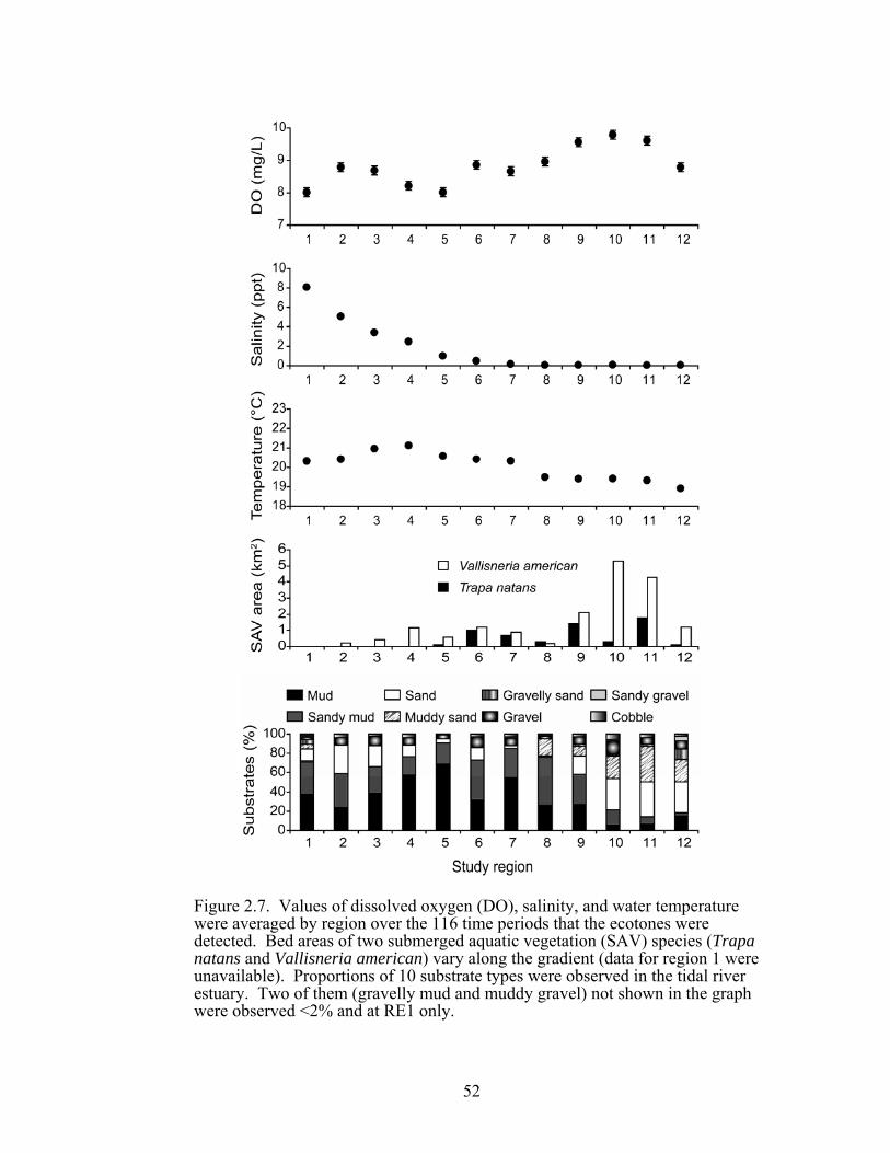
52
Figure 2.7. Values of dissolved oxygen (DO), salinity, and water temperature were averaged by region over the 116 time periods that the ecotones were detected. Bed areas of two submerged aquatic vegetation (SAV) species (Trapa natans and Vallisneria american) vary along the gradient (data for region 1 were unavailable). Proportions of 10 substrate types were observed in the tidal river estuary. Two of them (gravelly mud and muddy gravel) not shown in the graph were observed <2% and at RE1 only.

53
DISCUSSION
Formations of the Hudson ecotones were highly dynamic showing both shift in
location and change in structure over the detection periods (1974–2001). The ecotone
formations were related with the changes in habitat conditions over space and time.
Changeovers in fish species composition influencing by the transitions in
physicochemical conditions (Winemiller and Leslie 1992, Marshall and Elliott 1998,
Whitfield 1999, Martino and Able 2003) indicated the ecotone formations at the
particular portions on the Hudson River estuary gradient. Consistent with the study by
Attrill and Rundle (2002), the tidal Hudson River represents two important transitional
conditions between brackish and estuarine waters (from the lowest zone to the middle
zone of the gradient) and between estuarine and freshwater (from the middle zone to
the upper zone).Although the ecotone analysis was not determined at the lowest zone
(RE0) because of the unavailable fish data at this region prior to 1996, it is speculated
that the ecotone periphery between RE0 and RE1 is most likely to exist due to the
sharp transition between polyhaline and mesohaline waters (Weinstein et al. 1980)
between the two regions. At the lower zone, the sharp changes in DO and water
salinity between RE1 and RE2 apparently contributed to the formation of the ecotone
periphery (the narrow transition) that was highly detected between these two regions.
Salinity was not a major factor influencing formations of the ecotone peripheries at the
upper zone of the gradient where water condition becomes the tidal fresh (salinity
<0.5ppt; Winemiller and Leslie 1992).
At the upper gradient portion, the ecotone periphery frequently detected between
RE11 and RE12 was most likely influenced by the abrupt declines in DO and water
temperature from RE11 to RE12 in most months, the decreased abundance of Trapa
natans and Vallisneria americana from RE11 to RE12, and the dam constructions

54
above RE12 and in close proximity. Along the gradient, SAV occupied approximately
8% of the river bottom area, and 18% of the shallow water areas (≤3 m deep) was
available for SAV to colonize (Nieder et al. 2004). Below RE12, higher abundance of
the two SAV species, especially from RE9 to RE11, created both food sources and
shelters for inshore fish and other benthic animals in the shallow habitats (Abood and
Metzger 1996, Noordhuis et al. 2002, Strayer et al. 2004). In contrast, the dams
existing around and above RE12 alter flow regimes by reducing peak discharged
downstream and meting out flow over time to maintain minimum depths for
navigation (Lumia 1998). These consequences tend to affect distributions of fish
assemblages to the downriver portion (Abood and Metzger 1996, Schmidt and Cooper
1996).
While abrupt changes in both fish species composition and habitat conditions
concomitantly reflected the formations of ecotone peripheries between the particular
regions in the lower and upper zones, the ecotones were mainly detected within the
lower-middle zone of the gradient. The shift in locations of these ecotones, but still
within the gradient range from RE2 to RE5, tended to relate with the changes in
salinity regime, tidal current, and freshwater runoff seasonally or yearly (Weinstein et
al. 1980, Stanne et al. 1996, Attrill and Rundle 2002, Jaureguizar et al. 2003). Most of
the ecotones detected in the lower-middle zone had the breadth covering one or two
important nursery areas (i.e., Tappan Zee—RE2 and Haverstraw Bay—RE3) with low
salinity (1.0–5.1 ppt) serving diverse fish species (Stanne et al. 1996, Daniels et al.
2005) from marine (e.g., bay anchovy—Anchoa mitchilli and Atlantic menhaden—
Brevoortia tyrannus), estuarine (e.g., hogchoker—Trinectes maculates and banded
killifish—Fundulus diaphanus diaphanus), and freshwater (e.g., green sunfish—
Lepomis cyanellus and brown bullhead—Ameiurus nebulosus) assemblages.
55
However, in most time periods of the study, only one ecotone with the breadth
from RE2 to RE4 acted as an aggregator for most fish species, while the other
ecotones acted as soft or hard barriers for most of the Hudson fish (Table 2.1).
Furthermore, functional patterns of these ecotones on fish species assemblages were
not clearly different among seasons. From the comparison, while certain fish species
from marine, estuarine, and freshwater assemblages were usually observed in most
ecotones, total numbers of the fish species from the mixed assemblages in these
ecotones were intermediate or lower than those from the marine-estuarine or
freshwater assemblage observed in the adjacent habitat downstream or upstream,
respectively. Additionally, the abundance (numbers of individuals) of most fish
species was relatively low in the ecotones. These reflected complex distributions of
the Hudson fish assemblages and their variety of life histories (Hurst et al. 2004,
Daniels et al. 2005) responding to changing habitat conditions in and around the
ecotones on the gradient (Kupschus and Tremain 2001, Able 2005).
In an estuary, distributions of fish assemblages highly vary over short and long-
term periods due to: 1) complex life histories of fish and their habitat preferences that
may widely vary among life history stages (Able and Fahay 1998), 2) influences of the
recruitment dynamics of individual species (Hurst et al. 2004) and their differential
utilization of specific portions of the estuary (Weinstein et al. 1980), and 3) the
behaviors of fish that are inadequately understood (Able 2005). Along the Hudson
River estuary gradient, distributions of some fish species are restricted by their narrow
salinity tolerances, whereas distributions of other fish species with broader salinity
tolerances may be limited by other habitat variables that are correlated with salinity
concentration (Winemiller and Leslie 1992), e.g., tide, freshwater flow, and water
temperature (Vernberg and Vernberg 1976).

56
Influencing by river discharge and salinity concentration, young marine fish in the
Hudson system generally move upriver on the incoming flow of dense saline water
near the river bottom, whereas the young anadromous fish travel downriver on the
outgoing freshwater nearer the surface (Stanne et al. 1996). These fish assemblages
generally seek nursery areas with low salinity in the lower-middle zone of the tidal
river to temporarily spend their first year of life here and eventually migrate to the
Atlantic Ocean (Stanne et al. 1996, Able and Fahay 1998) as juveniles or adults
(Weinstein et al. 1980). For freshwater fish, some species may periodically move
farther downstream during high freshwater runoff with low salinity, while most
freshwater species are residents in the tidal fresh regions. Conclusively, patterns of
fish use of estuarine habitats in the lower-middle zone of Hudson is apparently a
continuum (Attrill and Rundle 2002, Able 2005); some species have obligated life
history stages (residents or diadromous) in the estuary, others are estuarine
opportunists, and still others are simply strays that occasionally find their ways into
the estuary (Able 2005).
The variations in freshwater flow, DO, salinity, and water temperature from month
to month also affected fish distributions (e.g., Gilmore 1995, Marshall and Elliott
1998, Whitfield 1999, Martino and Able 2003) in and around the Hudson ecotones.
During low freshwater flow with the increase salinity along the gradient, distribution
ranges of some marine and estuarine fish species show spatial change as they migrate
farther upstream (Attrill and Rundle 2002) beyond the brackish-estuarine ecotones (at
the lower-middle zone) leading to low species richness and abundance of fish in these
ecotones. In addition, both species richness and abundance of fish are mostly likely to
decrease at the freshwater-estuarine ecotones (at the middle-upper zone) of the
gradient as freshwater species became intolerant of increased salinity, while only a
few estuarine species can tolerate low salinity (Rundle at al. 1998).

57
Focusing at the lower-middle zone from RE2 to RE5 (where the ecotones were
highly detected), DO and water temperature showed gradual changes within the range
from RE2 to RE5 in a few months, but sharply fluctuated among these regions in most
months. Wells and Young (1992) found that the seasonal cycle accounted for most
(>99%) of the variation in water temperature in the Hudson system, whereas patterns
of changes in DO reflected an inverse relationship with water temperature (Mancroni
et al. 1992). Unlike DO and water temperature, salinity showed consistent pattern of
abrupt decrease from RE2 to RE5 in all study months, except in April. The synergy of
both gradual and sharp changes among these habitat variables plays important role in
structuring fish species assemblages (Whitfield 1999, Marshall and Elliott 1998) in
and around the Hudson ecotones. The bottom substrates are another factor influencing
distributions of fish species assemblages in an estuary at some extent (Weinstein et al.
1980). However, this habitat variable may play less influence on the distributions of
fish assemblages along the tidal Hudson River where the bottom of water is relatively
homogeneous. More than half of the gradient length (from RE1 to RE9) comprises a
major combination of mud and sandy mud, while sand and muddy sand were major
combined substrates at the remaining gradient length (RE10–RE12).
Since 1991, the zebra mussel invasion has been observed in the Hudson system
(Strayer et al. 1996) and its effect might be an additional factor shaping ecotone
functions on the Hudson fish species assemblages afterward. With their high filtration
rate of 6 m3/m2.day (Strayer et al. 1996), the zebra mussel populations are suspected to
bring about a selective decline in the density of phytoplankton and small zooplankton
(rotifers, tintinnids, and copepod nauplii) and a loss of consumers that depended on
phytoplankton and other edible particles in deep water of the Hudson (Pace et al.
1998, Strayer et al. 1999). In contrast, the filtration rates of the zebra mussel
populations increased sunlight penetration through surface of shallow water of the

58
Hudson enhancing the growth of aquatic plants and the invertebrates associated with
them (Strayer et al. 1999). These consequences interfered distribution patterns of the
Hudson fish assemblages and caused 28% of the median decrease in abundance of
open water fish species (e.g., Also spp.) due to the decline of food source in deep
water, but caused 97% of the median increase in abundance of littoral fish (e.g.,
sunfishes) due to the increase of food source in shallow water (Strayer et al. 2004). As
a result, both open-water and inshore fish assemblages move downstream and
upstream, respectively, away from the middle portion of the Hudson River estuary
gradient.
In conclusion, the formations of Hudson ecotones showed both changes in location
and structure spatially and temporally. In some time periods of detection, the ecotones
changed in their breadth (from broader to narrower or vice versa) or considerably
declined to be just ecotone peripheries. The ecotones were highly detected within the
lower–middle zone (RE2–RE5) of the Hudson River estuary gradient, whereas the
ecotone peripheries alone were highly detected at the lower zone (between RE1 and
RE2) and the upper zone (between RE11 and RE12) of the gradient. Abrupt changes
in one or more habitat variables and the peak turnover rates in fish species
composition were coincidently observed at the ecotone peripheries. Functional
patterns of the Hudson ecotones were not distinctly different across seasons. The
ecotone with the breadth from RE2 to RE4 was most likely to be the optimal zone for
distributions of diverse fish species assemblages, whereas the other ecotones acted as
barriers for most of the Hudson fish species. Likewise, the ecotone peripheries on the
gradient mainly inhibited distributions of most fish species between adjacent regions
with high contrast of habitat changes. Relatively low abundances of most fish species
observed in the Hudson ecotones were apparently related with complex migratory
behaviors and life histories of fish responding to variations in the estuarine conditions
59
in space and time. The effect of zebra mussel invasion in the Hudson system might be
an additional factor shaping the ecotone functions on distribution patterns of the
Hudson fish assemblages.
To explore influences of changing habitat in and around aquatic ecotones on
distributions of fish species assemblages in space and time, an explicitly abundance
exchange model was developed to quantify distribution patterns of target fish species
in association with their habitat preferences across lentic-lotic transitions on the two
freshwater gradients located on the southeastern coast of Lake Ontario. The
methodology of study, results, and discussion are presented in Chapter 3.

60
*CHAPTER THREE
An abundance exchange model of fish assemblage response to changing
habitat along embayment-stream gradients of Lake Ontario, New York
ABSTRACT
A spatially explicit abundance exchange model (AEM) was developed to predict
distribution patterns of five fish species in relation to their population characteristics
and habitat preferences along two embayment-stream gradients associated with Lake
Ontario, New York. The five fish species were yellow perch (Perca flavescens),
bluegill (Lepomis macrochirus), logperch (Percina caprodes), bluntnose minnow
(Pimephales notatus), and fantail darter (Etheostoma flabellare). Preference indexes
of each target fish species for water depth, water temperature, current velocity, cover
types (aquatic plants, algae, and woody debris), and bottom substrates (mud, sand,
gravel-cobble, and rock-bedrock) were estimated from the field observations, and
these were used to compute habitat preference (HP) of the associated fish species.
Fish HP was a key variable in the AEM to quantify abundance exchange of an
associated fish species among habitats on each study gradient. According to the
results, the AEM efficiently determined local distribution ranges of the fish species on
one study gradient. Results from the model validation showed that the AEM with its
estimated parameters was able to quantify most of the fish species distributions on the
second gradient. Overall, the AEM is rigorous for quantifying the distribution patterns
of the target species along the changing habitat gradients.
*Singkran, N., An abundance exchange model of fish assemblage response to changing habitat along embayment–stream gradients of Lake Ontario, New York, Ecol. Model. (2006), doi:10.1016/j.ecolmodel.2006.10.012

61
With its flexible structure that is applicable for array functions and differential
equations from both static and dynamic components, the AEM can be modified to
determine patterns of organism distribution in complex systems with different
environments and geography.
INTRODUCTION
The influence of changing landscapes and environments on organism distribution
across ecotones (transition zones) of contrasting habitats (e.g., grassland-forest) has
been increasingly studied in terrestrial ecosystems (e.g., Clements 1905, Leopold
1933, Odum 1971, Risser 1990, Johnson et al. 1992, Lidicker 1999, Fortin et al. 2000,
Harding 2002, Cadenasso et al. 2003, Ries et al. 2004), whereas fewer studies of this
similar research type have been conducted in aquatic ecosystems (Winemiller and
Leslie 1992, Willis and Magnuson 2000, Martino and Able 2003, Miller and Sadro
2003). Additionally, although distribution of organisms is a key mechanism
underlying the population dynamics (Nisbet and Gurney 1982, Tilman and Kareiva
1997), few empirical studies (Reyes et al. 1994, Gaff et al. 2000, Kupschus 2003) have
quantitatively determined organism distribution in association with both changes in
habitat and population characteristics (birth, death, and migration) over space and
time.
In this study, an abundance exchange model (AEM) was built to quantify the
distribution of fish species assemblages in relation to both population characteristics
and habitat preferences of fish across lentic-lotic transitions on two embayment-stream
gradients associated with Lake Ontario, New York. For purposes of this study, the
term “transition” referred to both abrupt and gradual changes in spatial habitat
heterogeneity between lentic (embayment) and lotic (stream) systems on the study

62
gradients. As a result, this transition is often distinctly observed at the lentic-lotic
periphery, and it may gradually or abruptly occur across the zone of transition between
the two systems.
The objectives of developing the spatially explicit AEM were to determine how
changing habitat influences distribution patterns of fish species assemblages along the
embayment-stream gradients and how population characteristics shape the size of fish
population over time. To test if the AEM could efficiently capture distribution
patterns of fish across different habitat conditions, five fish species, yellow perch
(Perca flavescens), bluegill (Lepomis macrochirus), logperch (Percina caprodes),
bluntnose minnow (Pimephales notatus), and fantail darter (Etheostoma flabellare)
were selected for modeling. Yellow perch and bluegill commonly distributed in the
embayment-downstream parts on both study gradients. Logperch was mainly
observed at the downstream-middle part on one study gradient, but this species was
not observed on the second gradient. Bluntnose minnow commonly distributed
throughout both study gradients, while fantail darter mainly distributed at the upstream
parts of both study gradients.
In aquatic systems, high variability in hydrology (Wiens 2002) and climate-linked
seasonal changes can alter other aquatic habitat variables (e.g., water temperature and
growth of aquatic plants and algae). As a result, the migration rate of fish along a
gradient is most likely to reflect fish habitat preference within a dynamic template.
Additionally, it has been considered that each fish species has a specific range of
distribution (e.g., Morrison et al. 1985, Guay 2000), the species stays within its range
but will variably distribute among habitats therein. This conforms to nonlinear
patterns of organism distribution along changing habitat gradients (Whittaker 1975,
Lewis 1997). In this study, both dynamic habitat variables (water depth, water
temperature, current velocity, aquatic plants, algae, and woody debris) and static

63
habitat variables (the bottom substrates, i.e., mud, sand, gravel-cobble, and rock-
bedrock) were observed along the study gradients and used to estimate fish habitat
preferences.
To test the hypothesis that distributions of fish across lentic-lotic transitions on the
study gradients are based on fish preferences for changing habitats within their local
ranges, habitat preferences of the target fish species at two life stages (0+ years and 1+
years) were the key variable in the AEM to quantify distribution patterns of the
associated fish species along each study gradient. STELLA® 7.0.3 Research (High
Performance Systems, Inc. 2002) was used to run the AEM. Since it was developed
by Barry Richmond in 1985, STELLA has been widely used by scientists across fields
of study. This software is capable of simulating many components and interactions of
complex systems, and is fast and efficient at calculating a diversity of array functions
and differential equations (e.g., Reyes et al. 1994, Pan and Raynal 1995, Marín 1997,
Gottlieb 1998, Ford 1999, Krivtsov et al. 2000, Dew 2001, Gertseva et al. 2003,
Gertseva et al. 2004, Kilpatrick et al. 2004, McCausland et al. 2006).
Besides model development and prediction, model validation, an important
modeling process (Haefner 1996, Olden et al. 2002, Ottaviani et al. 2004), was the
other objective of this study. Although numerous modeling approaches (e.g.,
statistics, system dynamics, and geographic information system (GIS)) have been used
for modeling species distribution, few of the models were further validated after the
predictions were completed (Olden et al. 2002). Model validation is crucial for
evaluating the accuracy of the model’s predictions and future applicability (Olden et
al. 2002, Ottaviani et al. 2004). In addition, proper ways of validating the model must
be implemented. To verify that the model prediction is robust and unbiased and has
minimal errors (i.e., over-fitting data, overrating model performance, or
underestimating the error for future application), one must validate the model with an

64
independent data set that has not been previously used to estimate the model’s
parameters (Guisan and Zimmermann 2000, Elith and Burgman 2002, Fielding 2002,
Olden et al. 2002, Ottaviani et al. 2004).
In this study, to evaluate if the AEM is robust and efficient for predicting the
distribution of the target fish species in similar geographic and hydrologic systems, the
model with its estimated parameters to quantify the distribution pattern of each target
species on one study gradient was validated against the observed data of the same fish
species on the second study gradient located in close proximity. Accuracy of the
model prediction was determined using the chi-square (χ2) statistic to test the
goodness of fit between predicted and observed percentage abundances of fish along
each study gradient. The important modeling processes and the model performance
presented in this study may contribute to applications for better predicting the
distribution of fish species assemblages across different habitats. This knowledge will
help resource managers evaluate and maximize healthy habitats among different
aquatic ecosystems to support diverse fish assemblages at both local and regional
scales.
STUDY GRADIENTS AND FIELD OBSERVATIONS
The empirical studies were conducted across lentic-lotic transitions on two
embayment-stream gradients, Floodwood (FL) and Sterling (ST) gradients, located on
the southeastern coast of Lake Ontario, New York (Figure 3.1). The FL gradient
comprises Floodwood Pond and Sandy Creek. The total watershed area for the FL
gradient was 671.82 km2, and the surface area of Floodwood Pond alone was 0.078
km2. Sandy Creek ranges in width from 6 m (upstream) to more than 50 m (entering
Floodwood Pond) and has a mean annual discharge of 7.8 m3/s (37-year record—

65
USGS gage 04250750 above study area). The ST gradient includes Sterling Pond and
Sterling Creek. The total watershed area associated with the ST gradient was 210.76
km2, and the surface area of Sterling Pond alone was 0.38 km2. Sterling Creek ranges
in width from 3 m (upstream) to more than 20 m (entering Sterling Pond) with a mean
annual discharge of 1.9 m3/s (37-year record—USGS gage 04232100 above study
area).
Figure 3.1. The Floodwood (FL) and Sterling (ST) gradients with eight sampling stations (stars, FL; circles, ST) for monthly collecting of target fish and habitat variables during June–August 2002. The fish and habitat collections were repeated at 12 stations (circles) along the FL gradient during June–August 2004.
A Garmin Etrex Venture global positioning system was used to mark locations of
sampling stations on both gradients. In the summer months (June–August) of 2002,
eight transect stations on the FL gradient (Figure 3.1: stars) were selected (between
43°43'16" N, 76°12'10" W and 43°48'47" N, 76°4'31" W) using a stratified random
sampling method to cover all habitat types. The length of the entire sampling gradient
was about 18.6 km. The same stratified random method was used to select eight
transect stations (between 43°20'34.5" N, 76°41'54.7" W and 43°16'51.6" N,

66
76°37'37.6" W) on the ST gradient (Figure 3.1). The length of the entire sampling
gradient was about 16.3 km.
Abundance of the five selected fish species (yellow perch, bluegill, logperch,
bluntnose minnow, and fantail darter) was observed once a month along the FL and
ST gradients during June–August 2002. Fish were randomly sampled for 15 minutes
per station at all FL and ST stations using electrofishing gear (the power supply to
generate electricity was a 3500-W generator and a transformer with DC voltage output
controller of 250–350 V). Juveniles and adults of each target species caught at each
station were enumerated and their total length was measured to the nearest millimeter.
In the same summer months, the habitat variables were measured once a month in
all stations where the fish species were collected as follows. Water depth (m) and
water temperature (°C) were randomly measured five times in each sampling station.
Current velocity (m/s) was randomly measured five times within each station using a
Marsh-McBirney 2000-model (Bovee 1982). Bottom substrates (%) were visually
observed once a month in all sampling fish stations on each study gradient; at the first
observation, substrate grain sizes (diameter) were measured and classified into four
types modified from Pusey et al. (1993): mud (<1 mm diameter), sand (1–16 mm
diameter), gravel-cobble (16–128 mm diameter), and rock-bedrock (>128 mm
diameter). The average percentage of each substrate type and average abundance of
each cover type was calculated from their 10 random observations in each station.
The abundance of aquatic plants, algae, and woody debris was coded on a scale of 0–
3: 0 = absent, 1 = low, 2 = common, and 3 = high.
In the summer months (June–August) of 2004, the fish and habitat collections
were repeated at 12 sampling stations (Figure 3.1: circles) along the FL gradient. The
12 sampling stations were located between 43°43'20.6" N, 76°12'13.3" W and
43°51'11.7" N, 75°56'44" W, the total sampling gradient length was 28.2 km. The

67
target fish species were sampled monthly at a total of 60 locations within the 12
stations along the FL gradient. With a fine scale of sampling, juveniles and adults of
each target species were collected for 10 minutes in each of the 60 locations using the
same fishing gear and sampling protocols as in the summer of 2002. Individuals of
each target fish species collected from all locations within each station were
accumulated, enumerated, and measured for total length to the nearest millimeter.
In the same summer months of 2004, the same habitat variables were sampled
monthly five times in each of the 60 locations within the 12 stations where the target
fish species were collected using the same methods and instruments as in the summer
of 2002. As a result, 900 samples for each habitat variable were collected along the
FL gradient during the three summer months of 2004. Mean values of each habitat
variable for the 180 samples along the FL gradient were then obtained by dividing the
total 900 samples by the five times of collection in each location (i.e., 900/5 = 180) in
summer 2004. The mean habitat variables and abundance data for the target fish
species collected on the FL gradient in the 2004 summer were used to build the AEM
and to estimate and calibrate the model’s parameters (i.e., a preference index of the
target fish species for each of the habitat variables). The model with its estimated
parameters was then validated against the fish and habitat data collected on the ST
gradient over the three summer months of 2002 (see detail in next section).
MODELING FISH DISTRIBUTIONS
ALONG EMBAYMENT-STREAM GRADIENTS
Applications of diffusion and random walk theories have been accepted as
powerful methods for spatially modeling organism dispersion (Nisbet and Gurney
1982, Reyes et al. 1994, Turchin 1998, Fagan et al. 1999, Kot 2001, Okubo and Levin

68
2001, Sparrevohn et al. 2002). In homogeneous habitat conditions, population
distribution of a given species in relation to certain habitat variables on a one-
dimensional gradient can be described as a Gaussian curve (Whittaker 1975, Lewis
1997). This normal distribution is the main idea proposed in Fick’s law of
particle/organism dispersion on a one-dimensional system expressed as (Okubo and
Levin 2001)
,22
2exp
2π0),( ⎟
⎟
⎠
⎞
⎜⎜
⎝
⎛−=
σ
xσ
ntxP (1)
where P(x, t) is the total individuals of a given species at location x and time t, n0 is the
initial number of individuals of a given species, and σ2 is the variance of the normal
distribution of a given species. It has been statistically proven that σ equals Dt2
(e.g., Fischer et al. 1979), where D is a constant dispersion rate (distance2/time) of the
population, and x is distance. Equation (1) after being rewritten becomes
⎟⎟
⎠
⎞
⎜⎜
⎝
⎛−
π=
Dtx
Dtn
txP4
2exp
40),( (2)
However, using a constant D in equation (2) may be unrealistic for describing
species distribution across heterogeneous habitat conditions (Johnson et al. 1992,
Fortin et al. 2000, Okubo and Levin 2001). In this study, it was assumed that the
migration rate of each target fish species varied depending on the fish preference for
changing habitat conditions across the lentic-lotic transition on each study gradient.
This assumption is based on the non-Fick’s law of dispersion (Johnson et al. 1992),

69
stating that although a given species acts as a random walker, it displays biased
decision to distribute to its optimal habitat.
Abundance exchange model development
A system dynamics approach, a rigorous modeling method that enables users to
build formal computer simulations of complex dynamic systems (Ford 1999, Sterman
2000) was used for building an abundance exchange model (AEM) to determine
distribution patterns of the target fish species along the two embayment-stream
gradients (Figure 3.1). The AEM includes both within-habitat and across-habitat
feedbacks to integrate population characteristics and habitat changes. The model
parameters were estimated and calibrated based on the fish and habitat data collected
along the FL gradient over the three summer months (June–August) of 2004. To
construct the AEM for each target fish species with respect to the species preference
for changing habitat, two major assumptions were made. First, distribution of the
target fish species at two life stages (0+ years and 1+ years) within and across habitats
on each study gradient was the result of functional migrations (Lucas and Baras 2001)
of fish to seek preferred areas for refuge in winter (November–March) and growth
(feeding and spawning) in growing season (April–October). Second, since small and
shallow waters can be conceptualized as one-dimensional habitats (Skalski and
Gilliam 2000), the distribution of each target fish species along the shallow gradients
(<6 m deep) was considered on one dimension only (i.e., in a horizontal direction from
downstream to upstream or vice versa).
The conceptual diagram (Figure 3.2) shows how the distribution pattern of each
target fish species within and across habitats was quantified along each study gradient.
From the diagram, fish that successfully overwinter in habitat n will migrate from
wintering areas to growing areas for breeding, feeding, or refuge in the growing

70
season. Mature fish will spawn at a certain period of time and have offspring in the
same season. In the late growing season, young fish will grow up and aggregate with
the adults to overwinter in the wintering areas. The same pattern of fish migration
within habitats is assumed to occur in habitat n–1 and n+1. Concurrently, migration of
a target fish species at both life stages also occurs among adjacent habitats.
Figure 3.2. A conceptual diagram of fish distribution within and among habitats. Migration rates of fish at two life stages in the growing season (yk, 0+ yr old; ak, 1+ yr old) and for all fish in winter (k) among habitats n, n–1, and n+1 are dependent on fish habitat preference in the growing season (yHP, 0+ yr old; aHP, 1+ yr old) and in winter (HP), respectively. The three graphs below show the estimated preference indexes (Pi) of the three example habitat variables that were used to compute the geometric mean HP for the target fish species at each life stage.
The migration rate (k) of each fish species varies in relation to the species habitat
preference (HP) along each study gradient. For instance, if a fish species preferred

71
habitat n–1 to habitat n, more individuals of that species would migrate to habitat n–1,
rather than stay in habitat n. In contrast, if suitable habitat conditions are not available
in habitat n–1 and n+1, the fish species’ populations are most likely to distribute only
within habitat n. In the AEM, the k of each target fish species among adjacent habitats
was derived from the fish species HP, such that k = (1–HP) over time t of the
simulation. The HP of each target species at each life stage is estimated using a
geometric mean model, equation (3), as follows.
NN
xx
/1
1PiHP ⎟⎟
⎠
⎞⎜⎜⎝
⎛= ∏
=, (3)
where Pix is a fish preference index (Degraaf and Bain, 1986) for each habitat variable
x. The model in equation (3) was employed from the habitat suitability index method
of Bovee (1986), which has been widely applied for determining health of fish habitats
(e.g., Pajak and Neves 1987, Reyes et al. 1994, Guay et al. 2000) and characterizing
species distributions (O’Connor 2002). In equation (3), Pix, is expressed as
)/()/(Pi
EtEjFtFj
x = (4)
where Fj is the number of individuals of a target fish species observed at an intensity
interval j of a habitat variable x, Ft is the total number of individuals of a target fish
species observed from all intensity intervals j of a habitat variable x, Ej is the number
of observations for a habitat variable x at an intensity interval j, and Et is the total
number of observations for a habitat variable x from all intensity intervals j.
To obtain the index between 0 and 1, the Pix on each interval j is normalized (i.e.,
Pix,j/Pix,jmax). Examples functions of the Piwater depth, Picurrent velocity, and Piwater temperature of

72
bluntnose minnow at both life stages in the growing season in habitat n–1 were shown
in Figure 3.2. The fish HP is then computed as a product of the fish species Pix for all
habitat variables N. To derive the HP value between 0 and 1 over time t of the
simulation, the HP, equation (3), is normalized with the power of 1/N. A summarized
equation incorporating both population characteristics and HP to simulate the AEM
for each target fish species along each study gradient is
{ } { }
),()(HPHP
HP)(HPHP
HP
)(HPHP
HP)(HPHP
HP
)()()()()(
n11
1
11
1
11
1
11
1
11111111
PrYykzyy
yAakzaa
a
Yykzyy
yAakzaa
a
YfYykAakYykAakdt
dP
dnnnn
nnn
nn
n
nnnn
nnn
nn
n
nn,nnn,nnn,nnn,nnn
×−⎭⎬⎫
⎩⎨⎧
××⎟⎟⎠
⎞⎜⎜⎝
⎛++
+××⎟⎟⎠
⎞⎜⎜⎝
⎛++
−
⎭⎬⎫
⎩⎨⎧
××⎟⎟⎠
⎞⎜⎜⎝
⎛++
+××⎟⎟⎠
⎞⎜⎜⎝
⎛++
−
+×+×+×+×=
+−
+
+−
+
+−
−
+−
−
++++−−−−
(5)
where Pn is the population of a target fish species in habitat n, and akn and ykn are
migration rates of 1+ year-old fish (A) and 0+ year-old fish (Y), respectively, out of
habitat n. Similarly, akn–1,n and akn+1,n are migration rates of A from habitat n–1 and
n+1, respectively, to habitat n, and ykn–1,n and ykn+1,n are migration rates of Y from
habitat n–1 and n+1, respectively, to habitat n. In this equation, akn equals (1–aHPn)
over time t. The rest of the migration rates are computed in the same way. The aHPn,
aHPn–1, and aHPn+1 are the HPs of A in habitats n, n–1, and n+1, respectively.
Likewise, the yHPn, yHPn–1, and yHPn+1 are the HPs of Y in habitats n, n–1, and n+1,
respectively.
A small number z (e.g., z ≤ 10–6) is added to the model to avoid zero denominators
in case the species HP in any habitat becomes zero at a certain time t of simulation.
The birth of a target species in habitat n, for example, is represented by a logistic
growth model, f(Yn), where f(Yn) equals rb × An × (1–Yn/Cy). That is, the birth of Yn
depends on An abundance, birth fraction rb, and carrying capacity Cy of Yn. The
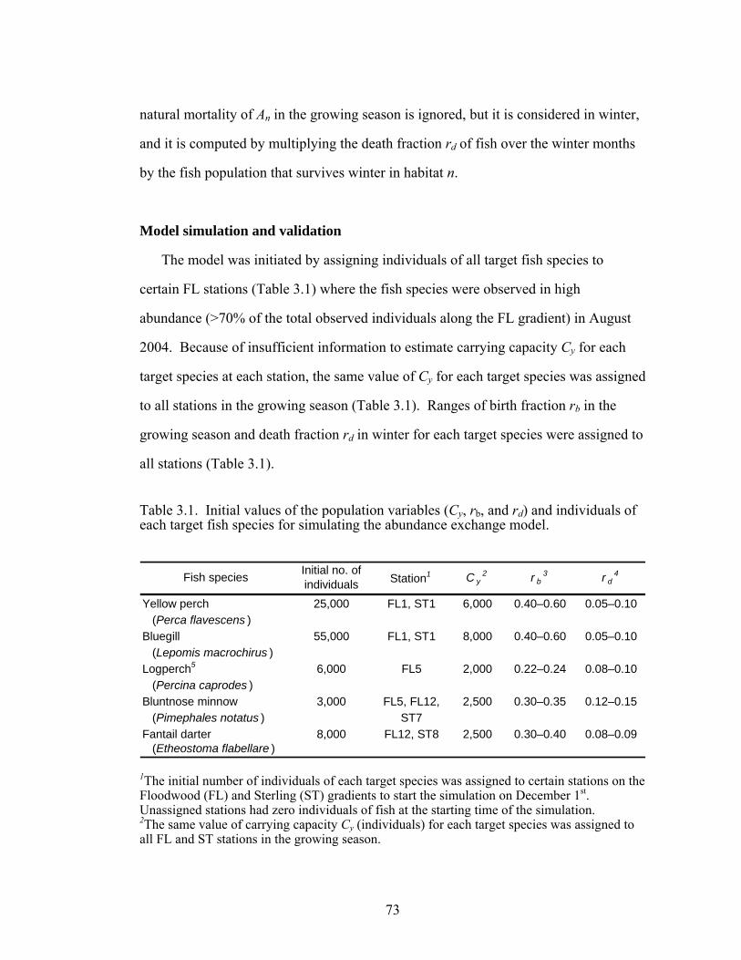
73
natural mortality of An in the growing season is ignored, but it is considered in winter,
and it is computed by multiplying the death fraction rd of fish over the winter months
by the fish population that survives winter in habitat n.
Model simulation and validation
The model was initiated by assigning individuals of all target fish species to
certain FL stations (Table 3.1) where the fish species were observed in high
abundance (>70% of the total observed individuals along the FL gradient) in August
2004. Because of insufficient information to estimate carrying capacity Cy for each
target species at each station, the same value of Cy for each target species was assigned
to all stations in the growing season (Table 3.1). Ranges of birth fraction rb in the
growing season and death fraction rd in winter for each target species were assigned to
all stations (Table 3.1).
Table 3.1. Initial values of the population variables (Cy, rb, and rd) and individuals of each target fish species for simulating the abundance exchange model.
Yellow perch 25,000 FL1, ST1 6,000 0.40–0.60 0.05–0.10 (Perca flavescens )Bluegill 55,000 FL1, ST1 8,000 0.40–0.60 0.05–0.10 (Lepomis macrochirus )Logperch5 6,000 FL5 2,000 0.22–0.24 0.08–0.10 (Percina caprodes )Bluntnose minnow 3,000 FL5, FL12, 2,500 0.30–0.35 0.12–0.15 (Pimephales notatus ) ST7Fantail darter 8,000 FL12, ST8 2,500 0.30–0.40 0.08–0.09 (Etheostoma flabellare )
r b3 r d
4Fish species Initial no. of individuals Station1 C y
2
1The initial number of individuals of each target species was assigned to certain stations on the Floodwood (FL) and Sterling (ST) gradients to start the simulation on December 1st. Unassigned stations had zero individuals of fish at the starting time of the simulation. 2The same value of carrying capacity Cy (individuals) for each target species was assigned to all FL and ST stations in the growing season.

74
Table 3.1 (Continued).
3The same range of birth fraction rb (month-1) for each target species was assigned to all FL and ST stations to generate series of uniformly distributed random values of rb in the growing season. 4The same range of death fraction rd (month-1) for each target species was assigned to all FL and ST stations to generate series of uniformly distributed random values of rd in winter. 5Distribution pattern of logperch was not modeled on the ST gradient.
From these initial conditions, the model generates series of uniformly distributed
random values of population variables for each fish species in the associated seasons.
To explore how the model would behave in a system in which a sharp change in each
population variable might occur for some reason (e.g., food increase/decline,
predator), ±50% changes in value of each population variable were assigned one at a
time at all FL stations to rerun the model.
Mean values of each habitat variable from the 180 samples along the FL gradient
were classified into intervals using natural breaks (Jenks), one of the classification
types in ArcGIS 9.1. This method is useful for a data set that contains relatively big
jumps in the data values. Thus, for each habitat variable, similar data values were
grouped together in the same interval, and the differences between intervals were
maximized. A fish species Pi for each habitat variable at each classified interval was
then estimated using equation (4) (Table 3.2).
Series of IF-THEN-ELSE statements (logical functions) were used to incorporate
the species Pi at each interval for all habitat variables (Table 3.2) into the AEM for
computing the species HP, equation (3). The species’ migration rate k in the model
was then converted from the species HP and used to quantify abundance exchange of
that species among FL stations in the growing season.

75
Table 3.2. Preference index (Pi) for each habitat variable of five modeled fish species at two life stages (0+yr and 1+yr old) estimated from the fish and habitat data observed along the Floodwood gradient over the three summer months (June–August) of 2004.
0+yr 1+yr 0+yr 1+yr 0+yr 1+yr 0+yr 1+yr 0+yr 1+yr
Water depth (m)0.10-0.3 0.10 0.16 0.17 0.10 1.00 1.00 0.62 1.00 1.00 0.730.31-0.6 0.03 0.00 0.17 0.02 0.17 0.29 0.75 0.43 0.73 1.000.61-1.0 0.00 0.00 0.00 0.00 0.00 0.00 1.00 0.61 0.49 0.771.01-4.0 1.00 1.00 1.00 1.00 0.37 0.09 0.08 0.22 0.00 0.00
Current velocity (m/s)0.03-0.06 1.00 1.00 1.00 1.00 0.19 0.00 0.05 0.12 0.00 0.000.07-0.12 0.18 0.46 0.59 0.90 1.00 1.00 1.00 1.00 0.92 0.680.13-0.24 0.04 0.00 0.07 0.06 0.66 0.91 0.48 0.41 0.37 0.700.25-0.36 0.04 0.00 0.00 0.06 0.76 0.86 0.64 0.60 1.00 1.000.37-0.48 0.00 0.00 0.00 0.00 0.00 0.00 0.00 0.00 0.13 0.42
Water temperature (°C)16.1-18 0.71 0.68 0.90 0.57 0.51 0.58 1.00 0.45 0.82 0.7418.1-20 1.00 0.45 1.00 0.27 1.00 1.00 0.59 0.73 1.00 1.0020.1-22 0.27 0.00 0.63 0.32 0.00 0.00 0.49 0.27 0.18 0.6622.1-24 0.30 0.27 0.00 0.28 0.51 0.00 0.19 0.10 0.05 0.1724.1-27 0.78 1.00 0.90 1.00 0.57 0.78 0.56 1.00 0.02 0.16
Aquatic plants1
0.01-0.3 0.00 0.00 0.00 0.00 0.00 0.00 0.65 0.64 1.00 1.000.31-0.6 0.01 0.00 0.04 0.08 0.11 0.12 1.00 0.39 0.36 0.680.61-1.0 0.54 0.94 0.31 0.82 1.00 1.00 0.59 1.00 0.01 0.031.01-1.5 0.33 0.25 0.00 1.00 0.00 0.00 0.00 0.00 0.00 0.001.51-3.0 1.00 1.00 1.00 0.99 0.00 0.00 0.00 0.31 0.00 0.00
Algae1
0.00-0.2 1.00 1.00 0.92 1.00 0.33 0.09 0.15 0.30 0.00 0.000.21-0.6 0.40 0.26 0.00 0.47 0.23 0.00 0.04 0.22 0.08 0.050.61-1.2 0.09 0.00 0.00 0.07 1.00 1.00 1.00 0.37 0.01 0.101.21-2.0 0.28 0.14 1.00 0.11 0.00 0.00 0.13 0.15 0.06 0.262.01-3.0 0.06 0.08 0.24 0.05 0.42 0.33 0.87 1.00 1.00 1.00
Woody debris1
0.01-0.3 0.08 0.00 0.00 0.08 1.00 1.00 0.35 0.93 1.00 1.000.31-0.6 0.22 0.22 0.54 0.33 0.46 0.62 1.00 1.00 0.48 0.910.61-1.0 0.88 0.52 0.17 0.58 0.28 0.00 0.28 0.23 0.02 0.181.01-1.5 1.00 1.00 1.00 1.00 0.00 0.00 0.08 0.17 0.00 0.00
Mud (%)0.0-5 0.04 0.08 0.11 0.04 0.51 0.52 0.62 1.00 1.00 1.005.1-15 0.08 0.00 0.24 0.06 0.56 1.00 1.00 0.34 0.01 0.07
15.1-30 0.25 0.47 0.29 1.00 1.00 0.24 0.13 0.41 0.00 0.0070.1-100 1.00 1.00 1.00 0.54 0.00 0.00 0.05 0.21 0.00 0.00
Fantail darterPi
Yellow perch Bluegill Logperch Bluntnose minnowHabitat variable
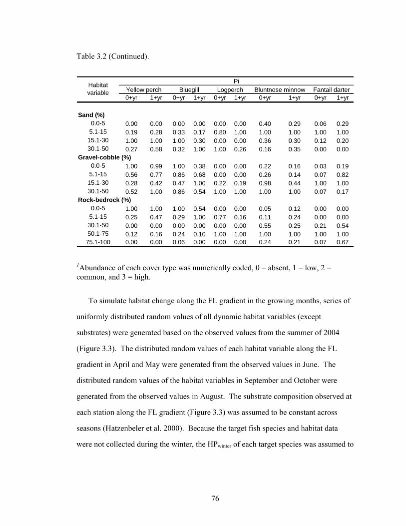
76
Table 3.2 (Continued).
0+yr 1+yr 0+yr 1+yr 0+yr 1+yr 0+yr 1+yr 0+yr 1+yr
Sand (%)0.0-5 0.00 0.00 0.00 0.00 0.00 0.00 0.40 0.29 0.06 0.29
5.1-15 0.19 0.28 0.33 0.17 0.80 1.00 1.00 1.00 1.00 1.0015.1-30 1.00 1.00 1.00 0.30 0.00 0.00 0.36 0.30 0.12 0.2030.1-50 0.27 0.58 0.32 1.00 1.00 0.26 0.16 0.35 0.00 0.00
Gravel-cobble (%)0.0-5 1.00 0.99 1.00 0.38 0.00 0.00 0.22 0.16 0.03 0.19
5.1-15 0.56 0.77 0.86 0.68 0.00 0.00 0.26 0.14 0.07 0.8215.1-30 0.28 0.42 0.47 1.00 0.22 0.19 0.98 0.44 1.00 1.0030.1-50 0.52 1.00 0.86 0.54 1.00 1.00 1.00 1.00 0.07 0.17
Rock-bedrock (%)0.0-5 1.00 1.00 1.00 0.54 0.00 0.00 0.05 0.12 0.00 0.00
5.1-15 0.25 0.47 0.29 1.00 0.77 0.16 0.11 0.24 0.00 0.0030.1-50 0.00 0.00 0.00 0.00 0.00 0.00 0.55 0.25 0.21 0.5450.1-75 0.12 0.16 0.24 0.10 1.00 1.00 1.00 1.00 1.00 1.0075.1-100 0.00 0.00 0.06 0.00 0.00 0.00 0.24 0.21 0.07 0.67
Habitat variable
PiYellow perch Bluegill Logperch Bluntnose minnow Fantail darter
1Abundance of each cover type was numerically coded, 0 = absent, 1 = low, 2 = common, and 3 = high.
To simulate habitat change along the FL gradient in the growing months, series of
uniformly distributed random values of all dynamic habitat variables (except
substrates) were generated based on the observed values from the summer of 2004
(Figure 3.3). The distributed random values of each habitat variable along the FL
gradient in April and May were generated from the observed values in June. The
distributed random values of the habitat variables in September and October were
generated from the observed values in August. The substrate composition observed at
each station along the FL gradient (Figure 3.3) was assumed to be constant across
seasons (Hatzenbeler et al. 2000). Because the target fish species and habitat data
were not collected during the winter, the HPwinter of each target species was assumed to

77
be the same as the species HP in the late growing season (October) estimated by the
model.
Figure 3.3. Categorized mean values of all habitat variables (except substrate composition) observed monthly during June–August 2002 along the Floodwood gradient. Abundance of aquatic plants, algae, and woody debris was rated from absent (0) to high (3). Percentage composition of four substrate types was averaged over the three months along the gradient.

78
The model was validated against the fish and habitat data collected on the ST
gradient in the summer of 2002. The AEM with all estimated Pi for each species from
the FL gradient was used to predict the distribution pattern of the same species (except
logperch) along the ST gradient. Logperch was not modeled on the ST gradient
because this species was not observed at all ST stations over the three summer months
(June–August 2002). To simulate the AEM on the ST gradient, the same individuals
of the target species assigned to the FL stations were assigned to the particular ST
stations (where the target fish species accounted for more than 70% of the total
observed individuals in August 2002) (Table 3.1). The same ranges of Cy, rb, and rd of
each modeled species assigned to the FL stations were also applied to all ST stations
(Table 3.1). Series of uniformly distributed values of the habitat variables along the
ST gradient in the growing months were generated from the values observed on this
gradient during the summer of 2002 (Figure 3.4) based on the same assumption made
for those on the FL gradient.
STELLA® 7.0.3 Research (High Performance Systems, Inc. 2002) was used to run
the AEM for a long-term prediction (100 hundred years) on each study gradient
starting with month 0 on December 1st and ending at 1,200 months on November 30th.
The interval of time between calculations (dt) was set to a small value of 0.0625
months to avoid artifactual delays and dynamics during the software calculation. The
artifactual delays result from the fundamental conceptual distinction between stocks
(state variables) and flows. Stocks exist at a point in time, whereas flows exist
between points in time. Consequently, the two components cannot coexist at the same
instant in time. For example, during migration of fish from one habitat to another
habitat, it will take an “instant” for fish from the first habitat to actually arrive in the
second habitat.

79
Figure 3.4. Categorized mean values of all habitat variables (except substrate composition) observed monthly during June–August 2002 along the Sterling gradient. Abundance of aquatic plants, algae, and woody debris was rated from absent (0) to high (3). Percentage composition of four substrate types was averaged over the three months along the gradient.

80
The “instant” constitutes the software’s artifactual delay. As long as dt is defined
as a relatively small value, the artifactual delays are usually insignificant (High
Performance Systems, Inc. 2002). Avoiding artifactual dynamics is the second reason
for choosing a small dt value for running the model that generates a dynamic pattern
of behavior caused by the way the software is performing its calculations. If the dt
value is too large, the flow volumes will be too large, and pathological results are
generated. However, the two problems are unlikely to occur when running the model
with the dt at or below 0.25 (High Performance Systems, Inc. 2002).
The chi-square (χ2) statistic was used to test the goodness of fit between the mean
predicted abundance (%) on August 31st from the 100-year simulation and the
observed abundance (%) of the target fish species in the same month on each study
gradient.
RESULTS
Model prediction
Populations of the five modeled fish species showed seasonal patterns of
distribution along the FL gradient over the 100-year simulation following results for
yellow perch (Figure 3.5). The fish populations declined in winter as a result of winter
mortality and increased in the growing season owning to birth and growth of
offspring. Populations were relatively stable for a certain time period in the growing
season after the spawning period when no offspring were born. After each growing
season, the fish populations rapidly declined during the subsequent winter. As
expected, the fish population size increased when higher value of either Cy (Figure
3.5B) or rb (Figure 3.5C), or lower value of rd (Figure 3.5D) was assigned one at a
time for simulating the model.

81
Figure 3.5: Seasonal distribution pattern of yellow perch over the 100-year simulation (A). The fish population size exponentially decreased or increased for the first 10-year period of the simulation when changes of 50% of carrying capacity Cy (B), birth fraction rb (C), or death fraction rd (D) were assigned to the abundance exchange model, but the population size returned to the seasonal pattern over the long-term prediction.
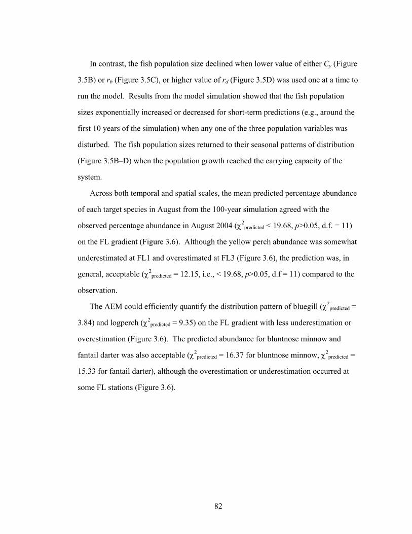
82
In contrast, the fish population size declined when lower value of either Cy (Figure
3.5B) or rb (Figure 3.5C), or higher value of rd (Figure 3.5D) was used one at a time to
run the model. Results from the model simulation showed that the fish population
sizes exponentially increased or decreased for short-term predictions (e.g., around the
first 10 years of the simulation) when any one of the three population variables was
disturbed. The fish population sizes returned to their seasonal patterns of distribution
(Figure 3.5B–D) when the population growth reached the carrying capacity of the
system.
Across both temporal and spatial scales, the mean predicted percentage abundance
of each target species in August from the 100-year simulation agreed with the
observed percentage abundance in August 2004 (χ2predicted < 19.68, p>0.05, d.f. = 11)
on the FL gradient (Figure 3.6). Although the yellow perch abundance was somewhat
underestimated at FL1 and overestimated at FL3 (Figure 3.6), the prediction was, in
general, acceptable (χ2predicted = 12.15, i.e., < 19.68, p>0.05, d.f = 11) compared to the
observation.
The AEM could efficiently quantify the distribution pattern of bluegill (χ2predicted =
3.84) and logperch (χ2predicted = 9.35) on the FL gradient with less underestimation or
overestimation (Figure 3.6). The predicted abundance for bluntnose minnow and
fantail darter was also acceptable (χ2predicted = 16.37 for bluntnose minnow, χ2
predicted =
15.33 for fantail darter), although the overestimation or underestimation occurred at
some FL stations (Figure 3.6).
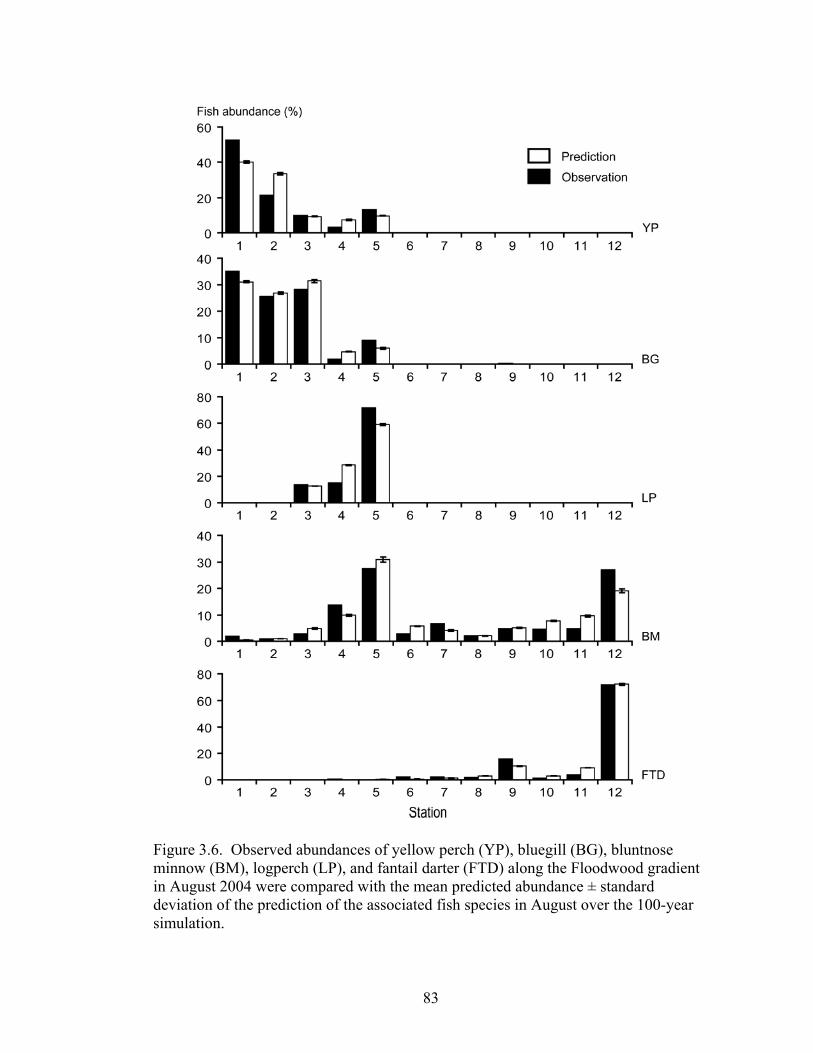
83
Figure 3.6. Observed abundances of yellow perch (YP), bluegill (BG), bluntnose minnow (BM), logperch (LP), and fantail darter (FTD) along the Floodwood gradient in August 2004 were compared with the mean predicted abundance ± standard deviation of the prediction of the associated fish species in August over the 100-year simulation.

84
The zero Pi of yellow perch (Table 3.2) for habitats with moderate-to-high
proportions of rock-bedrock above FL5 (Figure 3.3) limited the distribution of this
species to within FL1–FL5 as predicted by the model over the 100-year simulation
(Figure 3.7). The yellow perch population mainly aggregated at FL1 during winter
and early spring and migrated to FL2 in May and July, although a portion migrated to
FL4 and FL5. In the late growing season, most yellow perch moved downstream to
FL1 (Figure 3.7). Like yellow perch, the abundance exchange of bluegill occurred
between FL1 and FL5. The bluegill population mainly aggregated at FL1 during
winter and early spring. In June and July, bluegill were most abundant at FL2, but the
population spread to FL1 and FL3 in August, and most moved downstream to FL1 in
the late growing season (Figure 3.7).
The zero Pi of logperch for habitats containing high proportions of mud, such as
FL1–FL2, or moderate-to-high rock-bedrock content, such as FL6–FL12, defined the
distribution range of this species within FL3–FL5 (Figure 3.7). Logperch mainly
aggregated at FL4 and FL5 in the growing season, but at FL3 and FL4 in November
(Figure 3.7). Most fantail darter aggregated at the upstream portion on the FL gradient
across a year. Relatively few of them distributed to FL4 and FL5 in the growing
season (Figure 3.7). The distribution of fantail darter below FL4 (Figure 3.7) was
restricted by its zero Pi for habitats with little-to-no rock-bedrock content at FL1–FL3
(Figure 3.3). Unlike all other target species, bluntnose minnow distributed throughout
the FL gradient. In general, most bluntnose minnow aggregated at FL4, FL5, and
FL12 across a year (Figure 3.7).
85
Figure 3.7. Mean predicted abundance of yellow perch (YP), bluegill (BG), bluntnose minnow (BM), logperch (LP), and fantail darter (FTD) among months and stations on the Floodwood gradient over the 100-year simulation.

86
Model validation
The AEM with the estimated Pi for each target species on the FL gradient was
validated against the observed abundance of the same target species on the ST gradient
in the summer of 2002. The AEM predictions for yellow perch and fantail darter
agreed with the observations (Figure 3.8) along the ST gradient (χ2predicted < 14.07,
p>0.05, d.f. = 7).
Figure 3.8. Observed abundance of yellow perch (YP), bluegill (BG), bluntnose minnow (BM), and fantail darter (FTD) along the Sterling gradient in August 2002 were compared with the mean predicted abundance ± standard deviation of the prediction of the associated fish species in August over the 100-year simulation.

87
However, the model prediction was inconsistent with the observations of bluegill
and bluntnose minnow at some stations on the ST gradient. Significant differences
between predicted and observed abundances of bluegill occurred at ST7 and ST8
(χ2predicted > 3.84, p≤0.05, d.f. = 1). During the field sampling in August 2002, few
(6.3%) bluegill were observed at ST7 and fewer (3.1%) at ST8, while the average
abundance of bluegill over the 100-year simulation in the same summer month was
overestimated (16.2%) at ST7 and underestimated (0.3%) at ST8 (Figure 3.8).
Significant differences between predicted and observed abundances of bluntnose
minnow occurred at ST1 and ST3 (Figure 3.8). Few (3.5%) bluntnose minnow were
observed at ST1 and none at ST3 in August 2002, while the prediction of this species
was underestimated (0.3%) at ST1 and overestimated (4.7%) at ST3 (Figure 3.8).
According to the distribution patterns of the target species among months and ST
stations over the 100-year simulation (Figure 3.9), yellow perch distributed within the
range between ST1 and ST6, whereas bluegill distributed throughout the ST gradient
(Figure 3.9). Most yellow perch and bluegill aggregated at ST1 in winter and early
spring and migrated between ST1 and ST2 in the growing season. As on the FL
gradient, bluntnose minnow distributed throughout the ST gradient in the growing
season. Most of them aggregated at ST7 across a year (Figure 3.9). Predicted
distribution of fantail darter was between ST7 and ST8 across a year (Figure 3.9). In
general, the predicted abundance patterns of the modeled species in the summer
months were consistent with those from the field observations in the same time period.

88
Figure 3.9. Mean predicted abundance of yellow perch (YP), bluegill (BG), bluntnose minnow (BM), and fantail darter (FTD) among months and stations on the Sterling gradient over the 100-year simulation.

89
DISCUSSION
The modeled fish species showed relatively stable seasonal patterns of distribution
over the long-term prediction, and this was consistent with the findings of Reyes et al.
(1994), which revealed a stable seasonal pattern of pigfish abundance in Laguna de
Terminos, Mexico. The seasonal pattern of fish distribution can be explained in terms
of the negative and positive feedback loops (Ford 1999, Sterman 2000). The negative
feedback loop represents the contradictory conditions affecting fish distribution within
habitats between winter and the growing season, i.e., if more fish rapidly decline over
winter in these habitats, fewer fish will survive to have offspring or grow up in the
successive growing season. The positive feedback loop represents the supportive
condition increasing fish distribution within and across habitats between the two
seasons, i.e., if more young fish are born and more fish migrate from the other
habitats, a larger fish population in these habitats will be available to overwinter.
These consequences produced the seasonal patterns of fish distribution along Lake
Ontario’s coastal zone.
While the population variables (Cy, rb, and rd) shaped the population size of fish in
time, the model’s key variable, HP, accounted for fish distribution in space. As the
geometric mean of a species Pi for both static and dynamic habitat variables, HP could
capture the local range of species distribution and reflect the influence of habitat
changes (Morrison et al. 1985, Guay et al. 2000) on the abundance of a species within
its local range. Specifically, the estimated Pi (Table 3.2) for the static variable (i.e.,
substrate composition) defined the local distribution ranges of all modeled species on
the FL gradient and most of the species (except bluegill) on the ST gradient. Changes
in major substrate type(s) from a combination of mud and sand at FL3 to a
combination of gravel-cobble and rock-bedrock at FL4–FL5, and rock-bedrock at FL6

90
(Figure 3.3) marked these stations as the zone of transition in grain and extent
(Morrison and Hall, 2002) of the bottom landscape between lentic (embayment) and
lotic (stream) systems on the FL gradient. Similarly, changes in major substrate
type(s) from mud at ST6 to a combination of gravel-cobble and rock-bedrock at ST7
(Figure 3.4) indicated the distinct transition of the bottom landscape between the
lentic-lotic systems on the ST gradient.
In accordance with its local ranges of distribution in the upstream portions of
riffles and runs (Mundahl and Ingersoll 1983, Gray and Stauffer 1999) on both
gradients, fantail darter showed a high preference for shallow water, higher current
velocity, and rock-gravel streambeds (Table 3.2). In contrast, yellow perch and
bluegill represent embayment species that prefer deeper water habitat with common to
abundant aquatic plants and low current velocity (e.g., Harrington 1947, Wells 1968,
Helfman 1979, Hatzenbeler et al. 2000, Paukert and Willis 2002). Logperch
distributed within the lentic-lotic transition zone (FL3–FL5), habitats with moderate
current velocities, shallow water, and a combination of gravel-cobble and rock-
bedrock were preferred by this species (Smith 1985). Bluntnose minnow distributed
in a wide variety of water habitats (Trautman 1957, Becker 1983), but this species
preferred hard-bottomed, sandy, or gravelly shallows of pools for spawning activity
(Houston 2001) in the growing season. Consistently, high numbers of 0+year-old
bluntnose minnow were both observed and predicted at FL5 and FL12 that provide
suitable nursery substrates for this species.
Results from the model validation on the ST gradient revealed high levels of
agreement between the model predictions and the field observations for yellow perch
and fantail darter, but the predictions were not consistent with the observations for
bluegill and bluntnose minnow. The disagreement between predicted and observed
abundances of bluegill and bluntnose minnow at certain portions on the ST gradient

91
might be due to several causes. For bluntnose minnow, the small sample size (i.e., one
sample/station/month) of fish along the ST gradient might not well represent the
distribution pattern of this species along the gradient. Furthermore, increasing growth
of aquatic plants at the downstream and midstream portions of the gradient in the late
summer month could impede the ability to catch small fish. These factors might
explain why bluntnose minnow were not collected at most downstream-midstream
stations (ST3–ST6) on the ST gradient. Based on the broad tolerance of bluntnose
minnow for a wide variety of habitats, except the deeper waters of lakes and rivers
(Trautman 1957, Becker 1983), the model prediction revealed the distribution pattern
of this species throughout the ST gradient as being the same as that on the FL gradient.
The model parameters (i.e., Pi) for bluegill need some improvement to enhance the
ability of prediction on the ST gradient. Whereas this species was observed
throughout the ST gradient, results from the model simulation showed low efficiency
in quantifying abundance exchange of this species in the upstream portion of the
gradient. Pajak and Neves (1987) proposed three primary concerns that are generally
implicit in model validation procedures based on fish species Pi, one has to ensure that
(1) the fish species data to be validated are accurately collected, (2) the habitat
condition is accurately measured, and it is limited primarily by the habitat variables
included in the model, and (3) the sampling sites are representative sub-samples of the
target fish species’ habitats.
In this study, it is believed that methods of collecting both fish and habitat data
were appropriate. Nevertheless, it was noticeable that the sampling sites on the FL
gradient might not well represent all kinds of utilized substrates for bluegill on the ST
gradient. While the Pi for the rest of the habitat variables fell within the observed
ranges for bluegill on both study gradients, the Pi for substrate variables showed some
gaps between the quantified intervals (Table 3.2). This observation indicates that
92
although the substrates along the FL gradient were collected at a fine scale (900
samples), they were still unable to represent diverse proportions of the bottom
substrates occupied by bluegill on the ST gradient. Thus, the Pi for substrate variables
for this species may need to be improved for better model prediction. Similar gaps in
sampling coverage did not occur for the other modeled species.
Results from this study suggest that the species Pi for a given habitat variable
estimated from one study area may not completely represent the species Pi in another
study area (Pajak and Neves 1987, O’Connor 2002). Thus, to apply the AEM for
predicting fish species distribution in other water systems, one should crosscheck the
fish species Pi from existing data at both local and regional scales before incorporating
them into the AEM for computing the species HP. This is particularly necessary for
fish species with broad tolerances on the habitat variables that can powerfully define
local ranges of fish distribution (Hatzenbeler et al. 2000) or control distribution of fish
species from cell to cell (e.g., substrate types; Reyes et al. 1994). For different water
systems with different environmental conditions, influential habitat variables should
be considered for developing fish species Pi. Additionally, in large water systems
where fish movements in both vertical and horizontal directions are equally important,
two or more dimensions of fish distribution may need to be added in the model (e.g.,
Morrison et al. 1985, Reyes et al. 1994).
Overall, the AEM empirically developed from the fieldwork data performs rather
well for quantifying distributions of the coastal fish species assemblages along Lake
Ontario’s embayment-stream gradients. With its flexible model structure that can
accommodate array functions and multiple differential equations for both static and
dynamic components, the AEM can be modified to determine distribution patterns of
other types of organisms in different environmental and geographic systems.

93
Fish
spe
cies
RE
1R
E2
RE
3R
E4
RE
5R
E6
RE
7R
E8
RE
9R
E10
RE
11R
E12
Anad
rom
ous
Alew
ife24
6451
3258
5012
268
1353
014
429
7118
6885
4544
8302
7330
6382
(Alo
sa p
seud
ohar
engu
s)Am
eric
an s
had
1270
025
011
2908
633
150
3169
458
033
4465
729
278
2464
047
865
6385
845
563
(Alo
sa s
apid
issi
ma)
Atla
ntic
stu
rgeo
n0
70
00
30
014
717
30
0(A
cipe
nser
oxy
rinch
us
oxyr
inch
us)
Atla
ntic
tom
cod
1203
763
1415
2566
290
2110
70
10
4(M
icro
gadu
s to
mco
d)Bl
ueba
ck h
errin
g63
966
7261
145
225
1925
0118
8958
1661
1324
3664
2057
8014
9394
1437
8016
5875
1458
09(A
losa
aes
tival
is)
Hic
kory
sha
d3
90
90
00
00
10
2(A
losa
med
iocr
is)
Rai
nbow
sm
elt
1544
3027
1130
786
199
7412
310
664
1(O
smer
us m
orda
x m
orda
x)Se
a la
mpr
ey0
00
00
00
50
90
1(P
etro
myz
on m
arin
us)
Strip
ed b
ass
2725
960
760
5553
423
359
1501
611
946
7610
4969
6054
9021
1337
682
56(M
oron
e sa
xatil
is)
Cat
adro
mus
Amer
ican
eel
495
1919
1114
906
1038
1154
596
627
512
904
780
1824
(Ang
uilla
r ros
trata
)
App
endi
x 2.
1. C
umul
ativ
e ab
unda
nce
and
spec
ies r
ichn
ess o
f fis
h by
regi
on (R
E) a
long
the
Hud
son
Riv
er e
stua
ry
grad
ient
(RE1
–RE1
2) fr
om th
e fiv
e po
wer
pla
nt u
tiliti
es’ H
udso
n R
iver
est
uary
mon
itorin
g pr
ogra
m u
sing
bea
ch se
ine
surv
ey d
urin
g 19
74 to
200
1.

94
Fish
spe
cies
RE1
RE2
RE3
RE4
RE5
RE
6R
E7
RE
8R
E9
RE
10R
E11
RE
12
Est
uarin
eA
tlant
ic s
ilver
side
2047
395
912
6788
912
073
4011
1290
204
114
32
12
(Men
idia
men
idia
)B
ande
d ki
llifis
h95
7955
1642
131
796
4082
520
664
9930
8609
1677
418
514
3373
433
322
(Fun
dulu
s di
apha
nous
)Fa
t sle
eper
00
10
00
00
00
00
(Dor
mita
tor m
acul
atus
)Fo
ursp
ine
stic
kleb
ack
1516
4695
516
6826
9523
038
145
263
941
625
511
4(A
pelte
s qu
adra
cus)
Hog
chok
er24
1619
2314
3291
850
555
612
625
9512
936
525
(Trin
ecte
s m
acul
atus
)In
land
silv
ersi
de33
117
7417
7469
721
931
113
836
1089
4(M
enid
ia b
eryl
lina)
Mum
mic
hog
282
726
2782
2047
509
7030
1215
150
3050
1781
(Fun
dulu
s he
tero
clitu
she
tero
clitu
s)N
orth
ern
pipe
fish
996
4152
1607
283
305
00
00
06
(Syn
gnat
hus
fusc
us)
Sho
rtnos
e st
urge
on0
10
00
00
00
00
1(A
cipe
nser
bre
viro
stru
m)
Thre
espi
ne s
tickl
ebac
k11
3626
528
25
43
81
2(G
aste
rost
eus
acul
eatu
sac
ulea
tus)
Whi
te c
atfis
h14
1068
573
202
2639
3844
3546
2386
(Am
eiur
us c
atus
)
App
endi
x 2.
1 (C
ontin
ued)
.

95
Fish
spe
cies
RE1
RE2
RE3
RE4
RE5
RE
6R
E7
RE
8R
E9
RE
10R
E11
RE
12
Est
uarin
e (C
ontin
ued)
Whi
te m
ulle
t11
1311
210
03
00
20
0(M
ugil
cure
ma)
Whi
te p
erch
9677
7992
912
8023
4559
737
570
2709
922
055
2373
717
297
3874
041
222
1933
6(M
oron
e A
mer
ican
a)
Fres
hwat
erB
lack
bul
lhea
d0
01
00
00
01
10
0(A
mei
urus
mel
as)
Bla
ck c
rapp
ie0
1931
9028
4734
4430
5940
713
1(P
omox
is n
igro
mac
ulat
us)
Bla
ckno
se d
ace
1212
86
3920
40
00
254
(Rhi
nich
thys
atra
tulu
s)Bl
uegi
ll69
160
526
1047
810
1094
835
493
385
456
566
450
(Lep
omis
mac
roch
irus)
Blun
tnos
e m
inno
w0
02
02
00
31
26
87(P
imep
hale
s no
tatu
s)Br
idle
shi
ner
10
00
51
00
04
41
(Not
ropi
s bi
frena
tus)
Broo
k si
lver
side
00
00
00
00
00
410
0(L
abid
esth
es s
iccu
lus)
Broo
k st
ickl
ebac
k0
131
11
11
03
26
6(C
ulae
a in
cons
tans
)Br
ook
trout
00
20
00
10
00
00
(Sal
velin
us fo
ntin
alis
)
App
endi
x 2.
1 (C
ontin
ued)
.

96
Fish
spe
cies
RE1
RE2
RE3
RE4
RE5
RE
6R
E7
RE
8R
E9
RE
10R
E11
RE
12
Fres
hwat
er (C
ontin
ued)
Brow
n bu
llhea
d0
4775
942
572
815
038
310
699
9721
017
3(Ic
talu
rus
nebu
losu
s)B
row
n tro
ut1
34
15
41
01
02
5(S
alm
o tru
tta tr
utta
)C
entra
l mud
min
now
00
12
00
00
00
01
(Um
bra
limi)
Cha
in p
icke
rel
02
412
96
110
01
413
(Eso
x ni
ger )
Cha
nnel
cat
fish
00
01
02
25
23
21
(Icta
luru
s pu
ncta
tus)
Com
ely
shin
er0
00
02
230
01
00
17(N
otro
pis
amoe
nus)
Com
mon
car
p12
376
456
481
420
303
271
205
245
161
124
187
(Cyp
rinus
car
pio)
Com
mon
shi
ner
00
04
21
02
14
1812
0(N
otro
pis
corn
utus
)C
reek
chu
b0
180
24
35
71
02
5(S
emot
ilus
atro
mac
ulat
us)
Cut
lips
min
now
04
02
30
01
00
12
(Exo
glos
sum
max
illing
ua)
Eas
tern
mud
min
now
00
00
02
00
00
00
(Um
bra
pygm
aea)
Eas
tern
silv
ery
min
now
09
08
113
413
2931
4291
7510
(Hyb
ogna
thus
regi
us)
App
endi
x 2.
1 C
ontin
ued)
.

97
Fish
spe
cies
RE1
RE2
RE3
RE4
RE5
RE
6R
E7
RE
8R
E9
RE
10R
E11
RE
12
Fres
hwat
er (C
ontin
ued)
Em
eral
d sh
iner
238
4410
2615
411
987
123
105
387
1180
7355
(Not
ropi
s at
herin
oide
s)Fa
llfis
h0
50
03
25
102
1241
57(S
emot
ilus
corp
oral
is)
Fath
ead
min
now
01
00
62
33
819
227
(Pim
epha
les
prom
elas
)Fr
eshw
ater
dru
m0
01
00
00
01
30
0(A
plod
inot
us g
runn
iens
)G
izza
rd s
had
2294
194
354
1006
323
419
117
8072
7411
8(D
oros
oma
cepe
dian
um)
G
olde
n sh
iner
3313
810
2914
3353
4334
1758
1246
3426
3333
3315
1528
90(N
otem
igon
us c
ryso
leuc
as)
Gol
dfis
h10
8527
243
222
1244
170
660
982
054
146
940
2(C
aras
sius
aur
atus
aur
atus
)G
rass
pic
kere
l0
01
00
00
00
10
24(E
sox
amer
ican
us
verm
icul
atus
)G
reen
sun
fish
01
31
03
00
02
00
(Lep
omis
cya
nellu
s)La
rgem
outh
bas
s6
5421
599
527
965
846
161
031
623
115
616
9(M
icro
pter
us s
alm
oide
s)Lo
gper
ch0
01
00
01
21
42
8(P
erci
na c
apro
des)
App
endi
x 2.
1 (C
ontin
ued)
.

98
Fish
spe
cies
RE1
RE2
RE3
RE4
RE5
RE
6R
E7
RE
8R
E9
RE
10R
E11
RE
12
Fres
hwat
er (C
ontin
ued)
Long
ear s
unfis
h0
02
00
05
20
01
0(L
epom
is m
egal
otis
)Lo
ngno
se d
ace
00
04
11
00
00
24
(Rhi
nich
thys
cat
arac
tae)
Mim
ic s
hine
r0
00
00
00
10
00
1(N
otro
pis
volu
cellu
s)N
orth
ern
hog
suck
er2
00
01
32
13
413
4(H
ypen
teliu
m n
igric
ans)
Nor
ther
n pi
ke0
00
11
10
00
33
47(E
sox
luci
us)
Pug
nose
shi
ner
00
00
00
00
00
20
(Not
ropi
s an
ogen
us)
Pum
pkin
seed
1869
957
2465
7665
0854
9750
2567
0448
1136
8018
2915
78(L
epom
is g
ibbo
sus)
Rai
nbow
trou
t0
00
00
00
10
01
0(S
alve
linus
gai
rdne
ri )
Red
brea
st s
unfis
h3
4420
8173
319
959
115
4313
1510
3313
2374
966
5(L
epom
is a
uritu
s)R
edfin
pic
kere
l0
03
21
01
20
217
112
(Eso
x am
eric
anus
amer
ican
us)
Roc
k ba
ss1
15
73
221
1314
1715
156
(Am
blop
lites
rupe
stris
)
App
endi
x 2.
1 (C
ontin
ued)
.

99
Fish
spe
cies
RE1
RE2
RE3
RE4
RE5
RE
6R
E7
RE
8R
E9
RE
10R
E11
RE
12
Fres
hwat
er (C
ontin
ued)
Ros
yfac
e sh
iner
00
00
00
00
00
01
(Not
ropi
s ru
bellu
s)Sa
tinfin
shi
ner
00
00
83
03
75
2322
5(C
yprin
ella
ana
lost
ana)
Shie
ld d
arte
r0
00
00
00
10
00
0(P
erci
na p
elta
ta)
Smal
lmou
th b
ass
13
513
559
4179
151
159
158
346
(Mic
ropt
erus
dol
omie
ui)
Spo
tfin
shin
er0
37
117
3411
3316
1323
971
(Not
ropi
s sp
ilopt
erus
)Sp
otta
il sh
iner
509
1784
1211
320
052
5008
124
333
3554
641
154
2485
241
041
4202
776
124
(Not
ropi
s hu
dson
ius
)Sw
allo
wta
il sh
iner
00
00
10
03
02
02
(Not
ropi
s pr
ocne
)Te
ssel
late
d da
rter
3558
832
0381
4913
026
8656
5282
4509
6099
8386
5965
1571
7(E
theo
stom
a ol
mst
edi)
Tige
r mus
kellu
nge
00
00
00
00
00
11
(Eso
x lu
cius
cro
ss E
sox
mas
quin
ongy
)Tr
out-p
erch
00
00
00
00
00
040
(Per
cops
is o
mis
com
aycu
s)W
alle
ye0
00
00
00
10
03
0S
tizos
tedi
on v
itreu
m v
itreu
m)
App
endi
x 2.
1 (C
ontin
ued)
.

100
Fish
spe
cies
RE1
RE2
RE3
RE4
RE5
RE
6R
E7
RE
8R
E9
RE
10R
E11
RE
12
Fres
hwat
er (C
ontin
ued)
Whi
te b
ass
12
12
12
11
00
24
(Mor
one
chry
sops
)W
hite
cra
ppie
01
104
213
121
78
936
(Pom
oxis
ann
ular
is)
Whi
te s
ucke
r6
1618
337
914
311
814
075
3841
8322
1(C
atos
tom
us c
omm
erso
ni )
Yel
low
bul
lhea
d0
00
00
10
00
00
0(Ic
talu
rus
nata
lis )
Yello
w p
erch
116
181
453
274
133
177
196
151
149
148
659
(Per
ca fl
aves
cens
)
Mar
ine
Atla
ntic
cro
aker
3659
20
00
00
00
00
(Mic
ropo
goni
as u
ndul
atus
)A
tlant
ic h
errin
g50
00
00
00
00
00
0(C
lupe
a ha
reng
us h
aren
gus)
Atla
ntic
men
hade
n40
8627
076
2042
065
3533
1699
4422
4120
0130
3410
3767
5191
(Bre
voor
tia ty
rann
us)
Atla
ntic
moo
nfis
h1
30
00
00
00
00
0(S
elen
e se
tapi
nnis
)A
tlant
ic n
eedl
efis
h97
596
381
117
271
2650
2810
070
3155
(Stro
ngyl
ura
mar
ina)
Bay
anch
ovy
1934
2218
3599
2314
542
592
4129
945
8149
6055
652
063
147
38(A
ncho
a m
itchi
lli)
App
endi
x 2.
1 (C
ontin
ued)
.

101
Fish
spe
cies
RE1
RE2
RE3
RE4
RE5
RE
6R
E7
RE
8R
E9
RE
10R
E11
RE
12
Mar
ine
(Con
tinue
d)Bl
uefis
h37
5168
2365
9141
3520
7838
659
32
40
0(P
omat
omus
sal
tatri
x)Bu
tterfi
sh10
91
20
00
00
00
0(P
epril
us tr
iaca
nthu
s)C
reva
lle ja
ck52
136
149
218
223
40
00
00
(Car
anx
hipp
os)
Cun
ner
14
00
00
00
00
00
(Tau
togo
labr
us a
dspe
rsus
)Fo
ursp
ot fl
ound
er2
10
00
00
00
00
0(H
ippo
glos
sina
obl
onga
)G
oose
fish
00
01
00
00
00
00
(Lop
hius
am
eric
anus
)G
ray
snap
per
011
40
00
00
00
00
(Lut
janu
s gr
iseu
s)G
rubb
y0
10
00
00
00
00
0(M
yoxo
ceph
alus
aen
aeus
)In
shor
e liz
ardf
ish
1543
20
00
00
00
00
(Syn
odus
foet
ens)
Long
horn
scu
lpin
01
00
00
00
00
00
(Myo
xoce
phal
us
octo
dece
msp
inos
us)
Look
dow
n12
1913
20
00
00
00
0(S
elen
e vo
mer
)
App
endi
x 2.
1 (C
ontin
ued)
.

102
Fish
spe
cies
RE1
RE2
RE3
RE4
RE5
RE
6R
E7
RE
8R
E9
RE
10R
E11
RE
12
Mar
ine
(Con
tinue
d)N
aked
gob
y13
9017
174
21
00
00
0(G
obio
som
a bo
sc)
Nor
ther
n ki
ngfis
h12
313
712
00
00
00
00
0(M
entic
irrhu
s sa
xatil
is)
Nor
ther
n pu
ffer
824
60
00
00
00
00
(Sph
oero
ides
mac
ulat
us)
Nor
ther
n se
arob
in21
52
00
00
00
00
0(P
riono
tus
caro
linus
)N
orth
ern
star
gaze
r4
130
00
00
00
00
0(A
stro
scop
us g
utta
tus)
Ora
nges
potte
d fil
efis
h1
00
00
00
00
00
0(C
anth
erhi
nes
pullu
s)Pe
rmit
512
00
00
00
00
00
(Tra
chin
otus
blo
chii)
Red
hak
e0
00
00
00
20
00
0(U
roph
ycis
chu
ss)
Rou
gh s
ilver
side
286
879
677
217
341
10
10
21
(Mem
bras
mar
tinic
a)S
cup
00
10
00
00
00
00
(Ste
noto
mus
chr
ysop
s)S
eabo
ard
goby
00
10
00
00
00
00
(Gob
ioso
ma
gins
burg
i)S
ilver
hak
e3
00
069
00
00
00
0(M
erlu
cciu
s bi
linea
ris)
App
endi
x 2.
1 (C
ontin
ued)
.

103
Fish
spe
cies
RE1
RE2
RE3
RE4
RE5
RE
6R
E7
RE
8R
E9
RE
10R
E11
RE
12
Mar
ine
(Con
tinue
d)S
ilver
per
ch4
176
233
00
10
01
00
(Bai
rdie
lla c
hrys
oura
)S
mal
lmou
th fl
ound
er12
60
00
00
00
00
0(E
tropu
s m
icro
stom
us)
Spa
nish
mac
kere
l2
101
40
00
00
00
0(S
com
bero
mor
us m
acul
atus
)S
pot
656
564
351
476
8866
00
00
00
(Lei
osto
mus
xan
thur
us)
Spo
tfin
moj
arra
11
02
00
00
00
00
(Euc
inos
tom
us a
rgen
teus
)S
potte
d go
atfis
h0
00
00
00
00
00
17(P
seud
upen
eus
mac
ulat
us)
Spo
tted
hake
01
00
00
00
00
00
(Uro
phyc
is re
gia)
Stri
ped
anch
ovy
4319
74
20
00
00
00
(Anc
hoa
heps
ctus
)St
riped
killi
fish
10
00
00
00
00
00
(Fun
dulu
s m
ajal
is)
Stri
ped
mul
let
780
284
00
00
00
00
(Mug
il ce
phal
us)
Stri
ped
sear
obin
102
840
00
00
00
00
0(P
riono
tus
evol
ans)
Sum
mer
flou
nder
146
167
9326
106
00
00
00
(Par
alic
hthy
s de
ntat
us)
App
endi
x 2.
1 (C
ontin
ued)
.

104
Fish
spe
cies
RE
1R
E2R
E3R
E4R
E5R
E6R
E7R
E8R
E9
RE1
0R
E11
RE1
2
Mar
ine
(Con
tinue
d)Ta
utog
910
810
00
00
00
00
0(T
auto
ga o
nitis
)W
eakf
ish
247
244
2713
112
00
00
10
(Cyn
osci
on re
galis
)W
indo
wpa
ne7
10
00
00
00
00
0(S
coph
thal
mus
aqu
osus
)W
inte
r flo
unde
r92
984
250
70
20
00
00
0(P
seud
ople
uron
ecte
s am
eric
anus
)
Uni
dent
ified
spe
cies
Eso
x sp
p.0
00
00
00
00
00
1Fu
ndul
us s
pp.
00
10
00
00
01
00
unid
entif
ied
cent
rarc
hid
102
186
947
2252
3782
2942
1458
2775
3290
1096
540
2032
unid
entif
ied
clup
eid
1916
1254
521
5157
5428
828
4605
570
521
5837
190
574
8205
878
494
unid
entif
ied
cypr
inid
22
2010
873
917
136
119
613
410
861
1208
unid
entif
ied
gobi
id0
00
01
00
00
00
0un
iden
tifie
d M
oron
e0
11
186
31
01
40
78un
iden
tifie
d se
arob
in7
20
00
00
00
00
0un
iden
tifie
d st
urge
on0
00
00
02
00
00
0un
iden
tifie
d su
cker
00
00
00
30
00
03
unid
entif
ied
spp.
00
40
221
10
12
01
unid
entif
ied
spp.
00
30
00
00
00
00
unid
entif
ied
spp.
61
43
31
10
22
02
unid
entif
ied
spp.
07
7562
51
00
00
00
App
endi
x 2.
1 (C
ontin
ued)
.

105
Appendix 2.2. Multiple functions (aggregator, mediator, soft barrier, and hard barrier) of the ecotones (from all detected frequencies) on the Hudson fish species in each time period during 1974–2001.
Ecotone No. of selected1
location Aggregator Mediator Soft barrier Hard barrier species/gradient
RE2May-75 3.1 21.9 28.1 46.9 32May-76 6.7 26.7 26.7 39.9 30May-78 15.6 12.5 21.9 50.0 32Jun-74 8.8 11.8 20.6 58.8 34Jun-75 10.9 16.2 24.3 48.6 37Jun-76 12.2 9.8 34.1 43.9 41Jun-77 16.7 13.9 25.0 44.4 37Jul-78 7.0 18.6 14.0 60.4 43Jul-79 26.2 28.6 11.9 33.3 42Jul-84 31.0 21.4 9.5 38.1 42Jul-90 32.3 19.4 12.9 35.4 31Aug-78 10.2 18.4 20.4 51.0 49Aug-84 36.6 14.6 22.0 26.8 41Aug-96 21.4 10.7 17.9 50.0 28Sep-84 31.3 12.5 15.6 40.6 32Nov-76 18.2 13.6 22.7 45.5 22Nov-79 37.5 17.5 12.5 32.5 40Dec-78 0.0 11.1 27.8 61.1 18
RE2-RE3Jun-91 19.0 23.9 21.4 35.7 42Jul-00 20.0 17.1 8.6 54.3 35Sep-79 42.9 34.3 11.4 11.4 35Sep-81 27.9 9.3 23.3 39.5 43Sep-87 46.0 16.2 18.9 18.9 37Sep-99 12.5 6.3 18.8 62.4 32Oct-83 36.8 5.3 21.1 36.8 19Nov-78 16.7 33.3 13.3 36.7 30
RE2-RE4Jul-86 42.1 15.8 18.4 23.7 38Aug-74 22.0 30.0 22.0 26.0 50Aug-79 36.4 25.0 18.1 20.5 44Sep-82 38.5 25.6 18.0 17.9 39Sep-88 51.5 9.1 15.2 24.2 33Sep-96 30.0 20.0 30.0 20.0 20Oct-75 38.9 22.2 22.2 16.7 36Oct-98 22.6 19.4 6.5 51.5 31Nov-80 23.5 29.5 23.5 23.5 17Nov-86 36.0 28.0 12.0 24.0 25
Function (%) for the total selected species

106
Appendix 2.2 (Continued).
Ecotone No. of selected1
location Aggregator Mediator Soft barrier Hard barrier species/gradient
RE2-RE5Jun-94 9.4 12.5 28.1 50.0 32Aug-88 40.6 25.0 28.1 6.3 32Aug-90 56.3 15.6 18.7 9.4 32
RE2-RE6Jul-91 14.3 11.8 42.8 31.1 42Aug-87 30.3 15.2 33.3 21.2 33Sep-00 21.5 21.4 25.0 32.1 28
RE3Aug-96 25.0 17.9 25.0 32.1 28Sep-90 10.0 16.7 26.7 46.6 30
RE3-RE4Apr-74 50.0 11.1 16.7 22.2 18May-78 37.5 37.5 15.6 9.4 32Jun-75 29.8 40.5 10.8 18.9 37Jul-75 25.6 30.2 23.3 20.9 43Aug-81 18.0 35.9 28.2 17.9 39Aug-97 3.6 25.0 42.8 28.6 28Sep-01 3.5 13.8 24.1 58.6 29Oct-84 20.1 23.3 33.3 23.3 30Dec-78 38.9 27.8 11.1 22.2 18
RE3-RE5Aug-98 15.2 18.2 33.3 33.3 33Sep-98 7.0 10.3 37.9 44.8 29Oct-85 20.0 20.0 50.0 10.0 30Oct-92 21.4 25.0 14.3 39.3 28Nov-87 14.3 7.1 35.7 42.9 14
RE3-RE6May-76 60.0 16.6 6.8 16.6 30Aug-83 11.2 25.0 44.4 19.4 36Aug-91 4.7 20.9 37.2 37.2 43
RE4Jun-90 9.5 0.0 14.3 76.2 21
RE4-RE5Jul-90 3.2 9.7 12.9 74.2 31Aug-99 8.2 10.8 32.4 48.6 37Oct-83 15.8 26.3 31.6 26.3 19Oct-93 13.3 20.1 33.3 33.3 30Sep-81 4.7 9.3 44.2 41.8 43
Function (%) for the total selected species
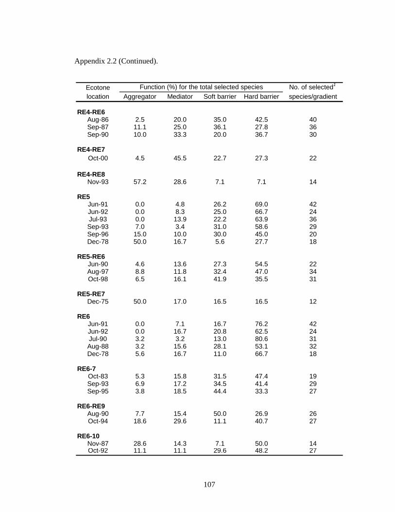
107
Appendix 2.2 (Continued).
Ecotone No. of selected1
location Aggregator Mediator Soft barrier Hard barrier species/gradient
RE4-RE6Aug-86 2.5 20.0 35.0 42.5 40Sep-87 11.1 25.0 36.1 27.8 36Sep-90 10.0 33.3 20.0 36.7 30
RE4-RE7Oct-00 4.5 45.5 22.7 27.3 22
RE4-RE8Nov-93 57.2 28.6 7.1 7.1 14
RE5Jun-91 0.0 4.8 26.2 69.0 42Jun-92 0.0 8.3 25.0 66.7 24Jul-93 0.0 13.9 22.2 63.9 36Sep-93 7.0 3.4 31.0 58.6 29Sep-96 15.0 10.0 30.0 45.0 20Dec-78 50.0 16.7 5.6 27.7 18
RE5-RE6Jun-90 4.6 13.6 27.3 54.5 22Aug-97 8.8 11.8 32.4 47.0 34Oct-98 6.5 16.1 41.9 35.5 31
RE5-RE7Dec-75 50.0 17.0 16.5 16.5 12
RE6Jun-91 0.0 7.1 16.7 76.2 42Jun-92 0.0 16.7 20.8 62.5 24Jul-90 3.2 3.2 13.0 80.6 31Aug-88 3.2 15.6 28.1 53.1 32Dec-78 5.6 16.7 11.0 66.7 18
RE6-7Oct-83 5.3 15.8 31.5 47.4 19Sep-93 6.9 17.2 34.5 41.4 29Sep-95 3.8 18.5 44.4 33.3 27
RE6-RE9Aug-90 7.7 15.4 50.0 26.9 26Oct-94 18.6 29.6 11.1 40.7 27
RE6-10Nov-87 28.6 14.3 7.1 50.0 14Oct-92 11.1 11.1 29.6 48.2 27
Function (%) for the total selected species

108
Appendix 2.2 (Continued).
Ecotone No. of selected1
location Aggregator Mediator Soft barrier Hard barrier species/gradient
RE7May-76 3.3 3.3 30.1 63.3 30
RE7-RE8Jun-90 33.3 14.3 9.5 42.9 21
RE7-RE9Dec-78 16.7 16.7 22.2 44.4 18
RE7-RE11Aug-87 21.2 27.3 18.2 33.3 33Aug-97 29.4 14.7 20.6 35.3 34Sep-87 19.4 22.3 19.4 38.9 36Sep-90 16.6 26.7 26.7 30.0 30Oct-88 27.6 6.9 31.0 34.5 29
RE8Aug-89 23.3 16.7 20.0 40.0 30Oct-00 4.5 9.1 18.2 68.2 22
RE8-9Apr-76 0.0 0.0 45.2 54.8 31
RE8-RE10Nov-85 13.1 30.4 17.4 39.1 23Dec-75 0.0 0.0 25.0 75.0 12
RE8-11Apr-78 4.0 8.0 40.0 48.0 25Sep-95 48.1 11.2 7.4 33.3 27
RE9Nov-77 2.9 2.9 26.6 67.6 34
RE9-RE10Jun-90 13.6 9.1 9.1 68.2 22Oct-00 22.7 22.7 22.7 31.9 22
RE9-RE11Nov-93 0.0 7.2 57.1 35.7 14
RE10-RE11Apr-76 0.0 6.5 32.3 61.2 31Nov-77 0.0 8.8 32.4 58.8 34
Function (%) for the total selected species

109
Appendix 2.2 (Continued).
Ecotone No. of selected1
location Aggregator Mediator Soft barrier Hard barrier species/gradient
RE11Jun-90 19.0 19.0 4.8 57.2 21Oct-92 11.1 7.4 22.2 59.3 27Oct-00 31.9 22.7 4.5 40.9 22Nov-87 21.4 14.3 0.0 64.3 14
Function (%) for the total selected species
1A fish species with less than 5 individuals collected along the Hudson River estuary gradient in each of the 116 time periods was not included in the analysis.
Appendix 2.3. Multiple functions (neutral, partly inhibit, and completely inhibit) of the ecotone peripheries (from all detected frequencies) on the Hudson fish species in each time period during 1974–2001.
Ecotone periphery No. of selected1
location between Neutral Partly inhibit Completely inhibit species/gradient
RE1-RE2Apr-78 8.0 20.0 72.0 25Apr-79 12.5 29.2 58.3 24May-74 26.1 4.3 69.6 23May-77 12.2 24.2 63.6 33Jun-78 12.5 20.0 67.5 40Jul-76 13.3 15.6 71.1 45Aug-80 12.2 9.8 78.0 41Aug-82 8.9 23.5 67.6 34Aug-89 10.0 10.0 80.0 30Aug-93 14.7 2.9 82.4 34Sep-75 8.3 22.9 68.8 48Sep-83 6.3 18.7 75.0 32Sep-85 11.8 23.5 64.7 34Sep-86 3.0 9.1 87.9 33Oct-74 11.8 17.6 70.6 34Oct-77 15.2 27.3 57.5 33Oct-81 16.7 13.9 69.4 36Nov-77 14.7 23.5 61.8 34
RE2-RE3Jun-79 13.9 44.4 41.7 36Jun-95 28.6 4.8 66.6 21Aug-75 11.1 31.1 57.8 45Nov-75 10.0 23.3 66.7 30
Function (%) for the total selected species

110
Appendix 2.3 (Continued).
Ecotone periphery No. of selected1
location between Neutral Partly inhibit Completely inhibit species/gradient
RE3-RE4Jun-88 17.1 17.1 65.8 35Jul-96 18.0 25.6 56.4 39Sep-76 18.0 41.0 41.0 36Sep-80 11.1 33.3 55.6 36Sep-94 8.6 17.1 74.3 35Oct-78 25.7 34.3 40.0 35Oct-80 15.4 26.9 57.7 26Oct-86 25.8 29.0 45.2 31Oct-95 13.3 30.0 56.7 30
RE4-RE5Sep-92 17.3 31.0 51.7 29
RE5-RE6Jul-97 8.6 40.0 51.4 35Jul-99 21.2 12.1 66.7 33Aug-94 16.2 29.0 54.8 31Aug-95 12.9 38.7 48.4 31
RE7-RE8Aug-00 14.3 40.0 45.7 35Oct-06 12.5 54.2 33.3 24
RE8-RE9Apr-79 16.7 25.0 58.3 24
RE10-RE11Jun-74 35.3 35.3 29.4 34Jun-78 22.5 35.0 42.5 40Jul-75 30.2 30.2 39.6 43Aug-79 29.5 29.5 41.0 44Sep-75 22.9 14.6 62.5 48Sep-80 30.6 19.4 50.0 36Oct-74 14.7 38.2 47.1 34Nov-80 11.8 5.9 82.3 17Nov-86 24.0 24.0 52.0 25
RE11-RE12May-74 13.1 21.7 65.2 23May-77 9.1 30.3 60.6 33May-78 21.9 18.7 59.4 32May-80 16.7 13.9 69.4 36Jun-79 13.9 16.7 69.4 36Jun-80 20.0 32.5 47.5 40Jun-95 9.6 33.3 57.1 21Jul-76 19.5 31.7 48.8 41Jul-77 14.0 25.5 60.5 43Jul-78 28.6 26.2 45.2 42
Function (%) for the total selected species

111
Appendix 2.3 (Continued).
Ecotone periphery No. of selected1
location between Neutral Partly inhibit Completely inhibit species/gradient
RE11-RE12 (Continued)Jul-97 8.6 20.0 71.4 35Jul-00 20.6 32.4 47.0 34Aug-75 20.0 28.9 51.1 45Aug-76 29.2 20.8 50.0 48Aug-78 28.6 22.4 49.0 49Aug-80 26.8 19.5 53.7 41Sep-76 25.6 18.0 56.4 39Sep-78 28.9 15.8 55.3 38Sep-79 22.9 22.9 54.2 35Sep-82 20.5 18.0 61.5 39Sep-94 20.0 20.0 60.0 35Sep-99 18.8 43.8 37.4 32Sep-01 16.7 13.3 70.0 30Oct-76 10.3 25.6 64.1 39Oct-78 20.0 11.4 68.6 35Oct-79 22.3 19.4 58.3 36Oct-80 15.4 26.9 57.7 26Oct-93 10.3 13.8 75.9 29Nov-78 16.7 10.0 73.3 30Nov-79 13.4 23.3 63.3 30
Function (%) for the total selected species
1A fish species with less than 5 individuals collected along the Hudson River estuary gradient in each of the 116 time periods was not included in the analysis.

112
REFERENCES
Able, K. W. 2005. A re-examination of fish estuarine dependence: evidence for
connectivity between estuarine and ocean habitats. Estuarine Coastal and Shelf Science 64:5–17.
Able, K. W., and M. P. Fahay. 1998. The first year in the life of estuarine fishes in the
middle Atlantic Bight. Rutgers University Press, New Brunswic, New Jersey.
Abood, K. A., and S. G. Metzger. 1996. Comparing impacts to shallow-water habitats
through time and space. Estuaries 19:220–228.
Armand, A. D. 1992. Sharp and gradual mountain timberlines as a results of species
interaction. Pages 360–378 in Hansen and di Castri, editors. Landscape boundaries: Consequences for biotic diversity and ecological flows. Springer-Verlag, New York.
ASA Analysis & Communication, I. 2004. 2001 year class report for the Hudson
River estuary monitoring program. Dynegy Roseton L.L.C., Entergy Nuclear Indian Point 2 L.L.C., Entergy Nuclear Indian Point 3 L.L.C., and Mirant Bowine L.L.C., New York.
Attrill, M. J., and S. D. Rundle. 2002. Ecotone or ecocline: ecological boundaries in
estuaries. Estuarine, Coastal and Shelf Science 55:929–936.
Baker, J., K. French, and R. J. Whelan. 2002. The edge effect and ecotonal species:
Bird communities across a natural edge in southeastern Australia. Ecology 83:3048–3059.
Barnthouse, L. W., R. J. Klauda, D. S. Vaughan, and R. L. Kendall, editors. 1988.
Science, law, and Hudson River power plants: a case study in environmental impact assessment. American Fisheries Society, Monograph 4, Bethesda, Maryland.
Becker, G. C. 1983. Fishes of Wisconsin. University of Wisconsin Press, Madison.

113
Bell, R. E., R. D. Flood, S. Carbotte, W. B. F. Ryan, F. O. Nitsche, S. Chilrud, R. Arko, V. Ferrini, A. Slagle, C. Bertinato, and M. Turrin. 2006. Hudson River estuary program benthic mapping project. Hudson River Estuary Program, New York State Department of Environmental Conservation, New York.
Bovee, K. D. 1982. A guide to stream habitat analysis using the instream flow
incremental methodology: Instream Flow Information Paper 5. FWS/OBS–82/26, U.S. Fish and Wildlife Service.
Bovee, K. D. 1986. Development and evaluation of habitat suitability criteria for use
in the Instream Flow Incremental Methodology. Instream Flow Information Paper 21: 86(7), U.S. Fish and Wildlife Service, Washington DC.
Bowersox, M. A., and D. G. Brown. 2001. Measuring the abruptness of patchy
ecotones. Plant Ecology 156:89–103.
Boyle, R. H. 1979. The Hudson River, Expanded edition. W.W. Norton and Company,
New York.
Cadenasso, M. L., S. T. A. Pickett, K. C. Weathers, and C. G. Jones. 2003. A
framework for a theory of ecological boundaries. BioScience 53:750–758.
Cadenasso, M. L., M. M. Traynor, and S. T. A. Pickett. 1997. Functional location of
forest edges: gradients of multiple physical factors. Canadian Journal of Forest Research 27:774–782.
Clements, F. E. 1897. Peculiar zonal formations of the Great Plains. American
Naturalist 31:968–970.
Clements, F. E. 1905. Research methods in ecology. University Pubishing Company,
Nebraska, USA.
Coch, N. K., and H. J. Bokuniewicz. 1986. Oceanographic and geologic framework of
the Hudson system. Northeastern Geology 8:96–108.
Csillag, F., B. Boots, M.-J. Fortin, K. Lowell, and F. Potvin. 2001. Multiscale
characterization of boundaries and landscape ecological patterns. Geomatica 55:291–307.

114
Daniels, R. A., K. E. Limburg, R. E. Schmidt, D. L. Strayer, and R. C. Chambers. 2005. Changes in fish assemblages in the tidal Hudson River, New York. American Fisheries Society Symposium 45:471–503.
Degraaf, D. A., and L. H. Bain. 1986. Habitat use by and preferences of Juvenile
Atlantic salmon in two Newfoundland Rivers. Transactions of the American Fisheries Society 115:671–681.
Delcourt, P. A., and H. R. Delcourt. 1992. Ecotone dynamics in space and time. Pages
19–54 in Hansen and di Castri, editors. Landscape Boundaries: Consequences for biotic diversity and ecological flows. Springer-Verlag, New York.
Dew, I. M. 2001. Theoretical model of a new fishery under a simple quota
management system. Ecological Modelling 143:59–70.
di Castri, F., and A. J. Hansen. 1992. The environment and development crises as
determinants of landscape dynamics. Pages 3–18 in Hansen and di Castri, editors. Landscape Boundaries: Consequences for biotic diversity and ecological flows. Springer-Verlag, New York.
di Castri, F., A. J. Hansen, and M. M. Holland, editors. 1988. A new look at ecotones:
emerging international projects on landscape boundaries (special issue 17). Biology International. IUBS, Paris, France.
Fagan, W. F., R. S. Cantrell, and C. Cosner. 1999. How habitat edges change species
interactions. American Naturalist 153:165–182.
Fagan, W. F., M. J. Fortin, and C. Soykan. 2003. Integrating edge detection and
dynamic modeling in quantitative analyses of ecological boundaries. BioScience 53:730–738.
Fielding, A. H. 2002. What are appropriate characteristics of an accuracy measure?
Pages 271–280 in Scott, Heglund, Morrison, and al., editors. Predicting species occurrences: issues of accuracy and scale. Island Press, Washington.
Fischer, H. B., E. J. List, R. C. Y. Koh, J. Imberger, and N. H. Brooks. 1979. Mixing
in inland and coastal waters. Academic Press, San Diego, California.

115
Ford, A. 1999. Modeling the Environment: an introduction to system dynamics modeling of environmental systems. Island Press, Washington, D.C.
Forman, R. T. T., and P. N. Moore. 1992. Theoretical foundations for understanding
boundaries in landscape mosaics. Pages 236–258 in Hansen and di Castri, editors. Landscape Boundaries: Consequences for biotic diversity and ecological flows. Springer-Verlag, New York.
Fortin, M.-J. 1994. Edge detection algorithms for two dimensional ecological data.
Ecology 75:956–965.
Fortin, M.-J., R. J. Olson, S. Ferson, L. Iverson, C. Hunsaker, G. Edwards, D. Levine,
K. Butera, and V. Klemas. 2000. Issues related to the detection of boundaries. Landscape Ecology 15:453–466.
Fruin, J. J. 1971. Pedestrian planning and design. Metropolitan Association of Urban
Designers and Environmental Planners, New York.
Gaff, H., D. L. DeAngelis, L. J. Gross, and R. Salinas. 2000. A dynamic landscape
model for fish in the Everglades and its application to restoration. Ecological Modelling 127:33–52.
Gauch, H. G., Jr. 1982. Multivariate analysis in community ecology, first edition.
Cambridge University Press, New York.
Gertseva, V. V., V. I. Gertsev, and N. Y. Ponomarev. 2003. Tropho-ethological
polymorphism of fish as a strategy of habitat development: a simulation model. Ecological Modelling 167:159–164.
Gertseva, V. V., J. E. Schindler, V. I. Gertsev, N. Y. Ponomarev, and W. R. English.
2004. A simulation model of the dynamics of aquatic macroinvertebrate communities. Ecological Modelling 176:173–186.
Gido, K. B., C. W. Hargrave, W. J. Matthews, and G. D. Schnell. 2002. Structure of
littoral-zone fish communities in relation to habitat, physical, and chemical gradients in a southern reservoir. Environmental Biology of Fishes 63:253–263.

116
Gilmore, R. G., Jr. 1995. Environmental and bigeographic factors influencing ichthyofaunal diverity in the Indian River Lagoon. Bulletin of Marine Science 57:153–170.
Gottlieb, S. J. 1998. Nutrient removal by age-0 Atlantic menhaden (Brevoortia
tyrranus) in Chesapeake Bay and implications for seasonal management of the fishery. Ecological Modelling 112:111–130.
Gray, E. V. S., and J. R. Stauffer, Jr. 1999. Comparative microhabitat use of
ecologically similar benthic fishes. Environ. Biol. Fishes. 56:443–453.
Guay, J. C., D. Boisclair, D. Rioux, M. Leclerc, M. Lapointe, and P. Legendre. 2000.
Development and validation of numerical habitat models for juveniles of Atlantic salmon (Salmo salar). Canadian Journal of Fisheries and Aquatic Science 57:2065–2075.
Guisan, A., and N. E. Zimmermann. 2000. Predictive habitat distribution models in
ecology. Ecological Modelling 135:147–186.
Haddad, N. M. 1999. Corridor use predicted from behaviors at habitat boundaries.
American Naturalist 153:215–227.
Haefner, J. W. 1996. Modeling biological systems: principles and applications.
Chapman & Hall, New York.
Hansen, A. J., and F. di Castri, editors. 1992. Landscape Boundaries: Consequences
for biotic diversity and ecological flows. Springer-Verlag, New York.
Hansen, A. J., F. di Castri, and R. J. Naiman. 1988. Ecotones: what and why? Pages 9-
45 in di Castri, Hansen, and Holland, editors. A new look at ecotones: emerging international project on landscape boundaries (special issue 17). Biological International, IUBS, Paris.
Harding, E. K. 2002. Modelling the influence of seasonal inter-habitat movements by
an ecotone rodent. Biological Conservation 104:227–237.
Harrington, R. W., Jr. 1947. Observations on the breeding habits of the yellow perch,
Perca flavescens (Mitchill). Copeia 1947:199–200.

117
Hatzenbeler, G. R., M. A. Bozek, M. J. Jennings, and E. E. Emmons. 2000. Seasonal variation in fish assemblage structure and habitat structure in the nearshore littoral zone of Wisconsin Lakes. North American Journal of Fisheries Management 20:360–368.
Helfman, G. S. 1979. Twilight activities of yellow perch, Perca flavescens. J. Fish.
Res. Board Can. 36:173–179.
High Performance Systems, Inc. 2002. STELLA(R) Research, version 7.0.3 for
Windows. Hanover, NH.
Hill, M. O. 1979. DECORANA: a FORTRAN program for detrended correspondence
analysis and reciprocal averaging. Cornell University, Ithaca, New York.
Hoeinghaus, D. J., K. O. Winemiller, and D. C. Taphorn. 2004. Compositional change
in fish assemblages along the Andean piedmont-Llanos floodplain gradient of the Rio Portuguesa, Venezuela. Neotropical Ichthyology 2:85–92.
Holland, M. M. 1988. SCOPE-MAB technical consultations of landscape boundaries:
report of a SCOPE/MAB workshop on ecotone, January 5–7, 1987. Pages 47–106 in di Castri, Hansen, and Holland, editors. A new look at ecotones: emerging international project on landscape boundaries (special issue 17). Biological International. IUBS, Paris.
Houston, J. 2001. Status of the bluntnose minnow, Pimephales notatus, in Canada.
The Canadian Field-Naturalist 115:145–151.
Hurst, T. P., K. A. McKown, and D. O. Conover. 2004. Interannual and long-term
variation in the Nearshore fish community of the mesohaline Hudson River estuary. Estuaries 27:659–669.
Jaureguizara, A. J., R. Mennic, C. Bremeca, H. Mianzan, and C. Lastaa. 2003. Fish
assemblage and environmental patterns in the Rio de la Plata estuary. Estuarine, Coastal and Shelf Science 56:921–933.
Johnson, A. R., J. A. Wiens, B. T. Milne, and T. O. Crist. 1992. Animal movements
and population dynamics in heterogeneous landscapes. Landscape Ecology 7:63–75.

118
Johnston, C. A., J. Pastor, and G. Pinay. 1992. Quantitative methods for studying landscape boundaries. Pages 107–125 in Hansen and di Castri, editors. Landscape Boundaries: Consequences for biotic diversity and ecological flows. Springer-Verlag, New York.
Johnston, V. R., and E. P. Odum. 1956. Breeding bird populations in relation to plant
succession on the piedmont of Georgia. Ecology 37:50–62.
Kilpatrick, H. J., A. M. LaBonte, J. S. Barclay, and G. Warner. 2004. Assessing
strategies to improve bowhunting as an urban deer management tool. Wildlife Society Bulletin 32:1177–1184.
Kirchhofer, A. 1995. Morphologicla variability in the ecotone–an important factor for
the conservation of fish species richness in Swiss rivers. Hydrobiologia 303:103–110.
Kolasa, J., and M. Zalewski. 1995. Notes on ecotone attributes and functions.
Hydrobiologia 303:1–7.
Kot, M. 2001. Elements of mathematical ecology. Cambridge University Press,
Cambridge, UK.
Krivtsov, V., Corliss, J., Bellinger, E., Sigee, D., 2000. Indirect regulation rule for
consecutive stages of ecological succession. Ecol. Model. 133, 73–81.
Kupschus, S. 2003. Development and evaluation of statistical habitat suitability
models: and example based on juvenile spotted seatrout Cynoscion nebulosus. Marine Ecology Progress Series 265:197–212.
Kupschus, S., and D. Tremain. 2001. Association between fish assemblages and
environmental factors in nearshore habitats of a subtropical estuary. Journal of Fish Biology 58:1383–1403.
Kupschus, S., and D. Tremain. 2001. Associations between fish assemblages and
environmental fiactors in nearshore habitats of a subtropical estuary. Journal of Fish Biology 58:1383–1403.

119
Lachavanne, J.-B. 1997. Why study biodiversity in land-inland water ecotones? Pages 1–33 in Lachvanne and Juge, editors. Biodiversity in land-inland water ecotones. UNESCO, Paris.
Lay, D. 1938. How valuable are woodland clearings to birdlife? Wilson Bulletin
50:254–256.
Leopold, A. 1933. Game management. Charles Scribner's Sons, New York.
Lewis, M. A. 1997. Variability, patchiness, and jump dispersal in the spread of an
invading population. Pages 46–69 in Tilman and Kareiva, editors. Spatial ecology: the role of space in population dynamics and interspecific interactions. Princeton University Press, Princeton, New Jersey.
Lidicker, W. Z. J. 1999. Responses of mammals to habitat edges: an overview.
Landscape Ecology 14:333–343.
Limburg, K. E., M. A. Moran, and W. H. McDowell. 1986. The Hudson River
ecosystem. Springer-Verlag, New York.
Lucas, M. C., and E. Baras. 2001. Migration of freshwater fishes. Blackwell Science,
London.
Lumia, R. 1998. Flood of January 19–20, 1996 in New York State. Water-Resources
Investigations Report, U.S. Geological Survey, Albany, New York.
Mancroni, W. J., M. W. Daley, and W. Dey. 1992. Recent Trends and Patterns in
selected water quality parameters in the mid-Hudson River estuary. Pages 59–81 in Smith, editor. Estuarine Research in the 1980s. State University of New York Press, Albany.
Marín, V. H. 1997. A simple-biology, stage-structured population model of the spring
dynamics of Calanus chilensis at Mejillones del Sur Bay, Chile. Ecological Modelling 105:65–82.
Marshall, S., and M. Elliott. 1998. Environmental Influences on the Fish Assemblage
of the Humber Estuary. Estuarine, Coastal and Shelf Science 46:175–184.

120
Martino, E. J., and K. W. Able. 2003. Fish assemblages across the marine to low salinity transition zone of a temperate estuary. Estuarine Coastal and Shelf Science 56:969–987.
Matthysen, E. 2002. Boundary effects on dispersal between habitat patches by forest
birds (Parus major, P. caeruleus). Landscape Ecology 17:509–515.
McCausland, W. D., E. Mente, G. J. Pierce, and I. Theodossiou. 2006. A simulation
model of sustainability of coastal communities: aquaculture, fishing, environment and labour markets. Ecological Modelling 193:271–294.
Miller, B. A., and S. Sadro. 2003. Residence time and seasonal movements of juvenile
coho salmon in the ecotone and lower estuary of Winchester Creek, South Slough, Oregon. Transactions of the American Fisheries Society 132:546–559.
Morrison, K. A., N. Therien, and B. Coupal. 1985. Simulating fish redistribution in the
LG-2 reservoir after flooding. Ecological Modelling 28:97–111.
Morrison, M. L., and L. S. Hall. 2002. Standard terminology: toward a common
languge to advance ecological understanding and application. Pages 43–52 in Scott, Heglund, Morrison, Haufler, Raphael, Wall, and Samson, editors. Predicting species occurrences. Island Press, Washington.
Mundahl, N. D., and C. G. Ingersoll. 1983. Early autumn movements and densities of
johny (Etheostoma nigrum)and fantail (E. Flabellare) darters in a southwestern Ohio stream. Ohio J. Sci. 83:103–108.
Naiman, R. J., and H. Décamps, editors. 1990. The ecology and management of
aquatic-terrestrial ecotones. The Parthenon Publishing Group, Paris.
National Oceanic and Atmospheric Administration. 1989. Estuaries of the United
States: vital statistics of a natural resource base. Strategic Environmental Assessments Division, Rockville, MD.
Neilson, R. P., G. A. King, R. L. DeVelice, and J. M. Lenihan. 1992. Regional and
local vegetation patterns: The responses of vegetation diversity to subcontinental air masses. Pages 129–149 in Hansen and Castri, editors. Landscape boundaries: Consequences for biotic diversity and ecological flows. Springer-Verlag, New York, New York.

121
Nieder, W. C., E. Barnaba, S. E. G. Findlay, S. Hoskins, N. Holochuck, and E. A. Blair. 2004. Distribution and abundance of submerged aquatic vegetation and Trapa natans in the Hudson River estuary. Journal of Coastal Research 45:150-161.
Nisbet, R. M., and W. S. C. Gurney. 1982. Modelling fluctuating populations. Jonh
Wiley & Son, New York.
Nitsche, F. O., R. Bell, S. M. Carbotte, W. B. F. Ryan, and R. Flood. 2004. Process-
related classification of acoustic data from the Hudson River Estuary. Marine Geology 209:131-145.
Noordhuis, R., D. T. van der Molen, and M. S. van den Berg. 2002. Response of
herbivorous watr-birds to the return of Chara in Lake Veluwemeer, the Netherlands. Aquatic Botany 72:349–367.
O'Connor, R. J. 2002. The conceptual basis of species distribution modeling: time for
a paradigm shift? Pages 25–33 in Scott, Heglund, Morrison, Haufler, Raphael, Wall, and Samson, editors. Predicting species occurrences. Island Press, Washington.
Odum, E. P. 1971. Fundamentals of ecology, third edition. W.B. Saunders Company,
Philadelphia.
Okubo, A., and S. A. Levin. 2001. Diffusion and ecological problems: Modern
perspectives, second edition. Springer, New York.
Olden, J. D., D. A. Jackson, and P. R. Peres-Neto. 2002. Predictive models of fish
species distributions: A note on proper validation and chance predictions. Transactions of the American Fisheries Society 131:329–336.
Ottaviani, D., G. J. Lasinio, and L. Boitani. 2004. Two statistical methods to validate
habitat suitability models using presence-only data. Ecological Modelling 179:417–443.
Pace, M. L., S. E. G. Findlay, and D. Fishcher. 1998. Effects of an invasive bivalve on
the zooplanktion community of the Hudson River. Freshwater Biology 39:103–116.

122
Pajak, P., and R. J. Neves. 1987. Habitat suitability and fish production: a model evaluation for rock bass in two Virginia streams. Transactions of the American Fisheries Society 116:839–850.
Pan, Y., and D. J. Raynal. 1995. Decomposing tree annual volume increments and
constructing a system dynamic model of tree growth. Ecological Modelling 82:299-312.
Paukert, C. P., and D. W. Willis. 2002. Seasonal and diel habitat selection by bluegills
in a shallow natural lake. Transactions of the American Fisheries Society 131:1131–1139.
Petts, G. E. 1990. The role of ecotones in aquatic landscape managment. Pages 227–
261 in Naiman and Decamps, editors. The ecology and managment of aquatic-terrestrial ecotones. UNESCO and The Parthenon Publishing Group, Paris, France.
Phillips, P. J., D. A. eckhardt, D. A. Freehafer, G. R. Wall, and H. H. Ingleston. 2002.
Regional patterns of pesticide concentration in surface waters of New York in 1997. Journal of the American Water Resources Association 38:731–745.
Pinay, G., H. Décamps, E. Chauvet, and E. Fustec. 1990. Functions of ecotone in
fluvial systems. Pages 141–169 in Naiman and Decamps, editors. The ecology and managment of aquatic-terrestrial ecotones. UNESCO and The Parthenon Publishing Group, Paris, France.
Przybylski, M., P. Biro, M. Zalewski, I. Tatrai, and P. Frankiewicz. 1991. The
structure of fish communities in streams of the northern part of the catchment area of Lake Balaton (Hungary). ACTA Hydrobiologica 33:135–148.
Pusey, B., A. H. Arthington, and M. G. Read. 1993. Spatial and temporal variation in
fish assemblage structure in the Mary River, south-eastern Queensland: the influence of habitat structure. Environmental Biology of Fishes 37:355–380.
Rakocinski, C. F., D. M. Baltz, and J. W. Fleeger. 1992. Correspondence between
environmental gradients and the community structure of marsh-edge fishes in a Louisiana estuary. Marine Ecology-Progress Series 80:135–148.
Reyes, E., F. H. Sklar, and J. W. Day. 1994. A regional organism exchange model for
simulating fish migration. Ecological Modelling 74:255–276.

123
Rhoads, D. C., and S. Cande. 1971. Sediment profile camera for in situ study of organism-sediment relations. Limnology and Oceanography 16:110–114.
Rhoads, D. C., and J. D. Germano. 1982. Characterization of organism-sediment
relations using sediment profile imaging: an efficient method of remote ecological monitoring of the seafloor (RemotsTM System). Marine EcologyProgress Series 8:115–128.
Ries, L., and D. M. Debinski. 2001. Butterfly responses to habitat edges in the highly
fragmented prairies of central Iowa. Journal of Animal Ecology 70:840–852.
Ries, L., R. J. Fletcher, Jr., J. Battin, and T. D. Sisk. 2004. Ecological responses to
habitat edges:mechanisms, models, and variability explained. Annual Reviews of Ecology, Evolution, and Systematics 35:491–522.
Risser, P. G. 1990. The ecological importance of land-water ecotones. Pages 7–21 in
Naiman and Decamps, editors. The ecology and managment of aquatic-terrestrial ecotones. Parthenon Publishing Group, Paris, France.
Ristich, S. S., M. Crandall, and J. Fortier. 1977. Benthic and epibenthic
macroinvertebrates of the Hudson River: Distribution, natural history and community structure. Estuarine, Coastal and Shelf Science 5:255–266.
Ross, J. A., S. F. Matter, and J. Roland. 2005. Edge avoidance and movement of the
butterfly Parnassius smintheus in matrix and non-matrix habitat. Landscape Ecology 20:127–135.
Rundle, S. D., M. J. Attrill, and A. Arshad. 1998. Seasonality in macroinvertebrate
community composition across a neglected ecological boundary, the freshwater-estuarine transition zone. Aquatic Ecology 32:211–216.
Schiemer, F., M. Zalewski, and J. E. Thorpe. 1995. The importance of aquatic-
terrestrial ecotones for freshwater fish. Hydrobiologia 303.
Schmidt, R. E., and S. Cooper. 1996. A catalog of barriers to upstream movement of
migratory fishes in Hudson River tributaries. Final report to Hudson River Foundation, New York.

124
Schmidt, R. E., R. J. Klauda, and J. M. Bartels. 1988. Distributions and movements of the early life stages of three species of alosa in the Hudson River, with comments on mechanisms to reduce interspecific completition. Pages 193–215 in Smith, editor. Fisheries research in the Hudson River. State University of New York Press, Albany, New York.
Sisk, T. D., and N. M. Haddad. 2002. Incorporating the effects of habitat edges into
landscape models: Effective area models for cross-boundary management. Pages 208–240 in Liu and Taylor, editors. Integrating landscape ecology into natural resource management. Cambride University Press, Cambridge, UK.
Sisk, T. D., and C. R. Margules. 1993. Habitat edges and restoration: methods for
quantifying edge effects and predicting the results of restoration efforts. Pages 45–55 in Saunders, Hobbes, and Ehrlich, editors. Nature conservertion 3: Reconstruction of fragmented ecosystems. Surrey Beatty and Sons Pty Limited Chipping Norton, New South Wales, Australia, Chipping Norton, New South Wales.
Skalski, G. T., and J. E. Gilliam. 2000. Modeling diffusive spread in a heterogeneous
population: a movement study with stream fish. Ecology 81:1685–1700.
Smith, C. L. 1985. The inland fishes of New York State. New York State Department
of Environmental Conservation, Albany, New York.
Sparrevohn, C. R., A. Nielsen, and J. G. Stottrup. 2002. Diffusion of fish from a single
release point. Canadian Journal of Fisheries and Aquatic Science 59:844–853.
Stamps, J. A., M. Buechner, and V. V. Krishnan. 1987. The effects of edge
permeability and habitat geometry on emigration from patches of habitat. American Naturalist 129:533–552.
Stanne, S. P., R. G. Panetta, and B. E. Forist. 1996. The Hudson. Rutgers University
Press, New Brunswick, New Jersey.
Sterman, J. D. 2000. Business dynamics: Systems thinking and modeling for a
complex world. McGraw-Hill, Singapore.
Strayer, D. L., N. F. Caraco, J. J. Cole, S. Findlay, and M. L. Pace. 1999.
Transformation of freshwater ecosystems by bivalves. BioScience 49:19–27.

125
Strayer, D. L., K. A. Hattala, and A. W. Kahnle. 2004. Effects of an invasive bivalve (Dreissena polymorpha) on fish in the Hudson River estuary. Canada Journal of Fisheries and Aquatic Science 61:924–941.
Strayer, D. L., J. Powell, P. Ambrose, L. C. Smith, M. L. Pace, and D. T. Fischer.
1996. Arrival, spread, and early dynamics of a zebra mussel (Dreissena polymorpha) population in the Hudson River estuary. Canada Journal of Fisheries and Aquatic Science 53:1143–1149.
Strayer, D. L., M. E. Power, W. F. Fagan, S. T. A. Pickett, and J. Belnap. 2003. A
classification of ecological boundaries. BioScience 53:723–729.
ter Braak, C. J. F., and P. Smilauer. 1998. Canoco reference manual and user's guide
to Canoco for windows: Software for canonical community ordination (version 4). Microcomputer Power, Ithaca, New York.
Texas Instruments, I. 1976. 1975 Water qualtity standard operating procedures.
Consolidated Edison Company of New York, New York.
Texas Instruments, Inc. 1977. 1974 year-class report for the multiplant impact study of
the Hudson River estuary. Consolidated Edison Company of New York, New York.
Texas Instruments Inc. 1981. 1979 year class report for the muliplant inmpact study of
the Hudson River estuary. Consolidated Edison Company of New York, New York.
Tilman, D., and P. Kareiva, editors. 1997. Spatial ecology: the role of space in
population dynamics and interspecific interaction. Princeton University Press, Princeton, New Jersey.
Trautman, M. B. 1957. The fishes of Ohio. Ohio State University Press, Columbus,
Ohio.
Turchin, P. 1998. Quantitative analysis of movement: measuring and modeling
populaiton redistribution in animals and plants. Sinauer Associates, Inc., Sunderland, Massachusetts.

126
Vernberg, W. B., and F. J. Vernberg. 1976. Physicological adaptations of estuarine animals. Oceanus 19:48–54.
Wagner, C. M. 1999. Expression of the estuarine species minimum in littoral fish
assemblages of the lower Chesapeake Bay tributaries. Estuaries 22:304–312.
Wall, G. R., and P. J. Phillips. 1998. Pesticides in the Hudson River basin, 1994–96.
Northeastern Geology and Environmental Sciences 20: 299–307.
Ward, J. V., and J. A. Stanford. 1983. The serial discontinuity concept of lotic
ecosystems. Pages 347–356 in Fontaine and Bartell, editors. Dynamics of lotic ecosystems. Ann Arbor Science Publishers, Ann Arbor, MI.
Watson, J. E. M., R. J. Whittaker, and T. P. Dawson. 2004. Habitat structure and
proximity to forest edge affect the abundance and distribution of forest-dependent birds in tropical coastal forests of southeastern Madagascar. Biological Conservation 120:311–327.
Weinstein, M. P., S. L. Weiss, and M. F. Walters. 1980. Multiple determinants of
community structure in shallow marsh habitats, Cape Fear River estuary, North Carolina. Marine Biology 58:227–243.
Wells, A. W., and J. R. Young. 1992. Long-term variability and predictability of
Hudson River physical and chemical characteristics. Pages 29–58 in Smith, editor. Estuarine research in the 1980s. State University of New York Press, Albany, New York.
Wells, L. 1968. Seasonal depth distribution of fish in southeastern Lake Michigan.
Fisheries Bulletin 67, U.S Fish and Wildlife Service.
Whitfield, A. K. 1999. Ichthyofaunal assemblages in estuaries: A South African case
study. Reviews in Fish Biology and Fisheries 9:151–186.
Whittaker, R. H. 1975. Communities and Ecosystems, second edition. Macmillan
Publishing, New York.
Wiens, J. A. 1992. Ecological flows across landscape boundaries: a conceptual
overview. Pages 217–235 in Hansen and di Carstri, editors. Landscape boundaries:

127
Consequences for biotic diversity and ecological flows. Springer-Verlag, New York, New York, USA.
Wiens, J. A. 2002. Riverine landscapes: taking landscape ecology into the water.
Freshwater Biology 47:501–515.
Wiens, J. A., C.S.Crawford, and J.R.Gosz. 1985. Boundary dynamics: a conceptual
framework for studying landscape ecosystems. Oikos 45:421–427.
Wiens, J. A., N. C. Stenseth, B. Van Horne, and R. A. Ims. 1993. Ecological
mechanisms and landscape ecology. Oikos 66:369–380.
Willis, T. V., and J. J. Magnuson. 2000. Patterns in fish species composition across the
interface between streams and lakes. Canadian Journal of Fisheries and Aquatic Science 57:1042–1052.
Winemiller, K. O., and M. A. Leslie. 1992. Fish assemblages across a complex,
tropical freshwater/marine ecotone. Environmental Biology of Fishes 34:29–50.
Zalewski, M. 1997. Fish diversity and ecotonal habitat. Pages 183-203 in Lachavanne
and Juge, editors. Biodiversity in land-inland water ecotones. UNESCO and The Parthenon Publishing Group, Paris.
Zalewski, M., J. E. Thorpe, and R. J. Naiman. 2001. Fish and riparian ecotones-a
hypothesis. Ecohydrology and Hydrobiology 1:11–14.