Ecosystem ecology and sustainability in

the Chinampa raised-field agriculture of

Mexico City

A Master of Science thesis in

Environmental Risk

by

Jorge Federico Miranda Vélez

Supervisor: Niels H. Jensen

Institute for Nature and Environment

Roskilde University

September 2018

i

Foreword

I feel genuine pity for the poor souls who will read this thesis. They’ll drag themselves through page after page of dark references and impossibly convoluted approximations about the ecosystem ecology of carbon in the 15th-century Chinampas of central Mexico, an environment they likely just heard about for the first time, and then, after what seemed an eternity of squinting and drinking strong coffee, they’ll make it to the end, teary-eyed and gasping for air, only to turn the page and read the heading:

"Nitrogen"

Acknowledgements

I suppose it’s only fair to name all the people that are to blame for this particular piece of work. After all, I can’t be responsible for all of it:

My supervisor, Niels, for trusting me with this whole thing, but mostly for showing me how much of our world is contained within the soil we grow on. My loving wife, Nika, for putting up with my endless rants about nitrogen fluxes and even proof-reading the whole manuscript, and in general for refusing to let me starve myself to death in the living room armchair, typing this thesis on nothing but coffee. Katrine, Rikke, Torben and Anne, for not shooing me out of their laboratories with a broom, but instead helping me with my poorly-timed questions and requests. And finally, Diego, Maya, Leo and Armando from Humedalia A.C. for sharing their time, their space, their soil and their love for the wetlands of Xochimilco. This thesis would’ve never been written were it not for them.

ii

Abstract

This thesis presents an analysis of the prehispanic and modern chinampas of central Mexico through

the lens of ecosystem ecology and soil science, aimed at gauging the actual richness and

sustainability of this agricultural practice. To do so, it makes use of historical accounts and modern

archaeological findings to reconstruct a cohesive conceptual model of what the Chinampa

agricultural system, as well as the chinampa raised fields themselves, likely looked like in the late

15th century A.D. Onto this conceptual model, the Chinampa’s original ecosystem ecology is overlaid

by calculating pools and fluxes of carbon, nitrogen and phosphorus from known aspects of this

agricultural system; and where detailed ecological knowledge is lacking, historical accounts and

parallel ecosystems are brought in to fill in the gaps through extrapolation and inference.

These conceptual models and theoretical nutrient cycles are brought closer to the ground by the

combination of field work performed in the late 2017 and early 2018 in the extant chinampas of

Xochimilco, Mexico, and subsequent laboratory analyses of soil and sediment samples collected in

the field.

The analyses, performed at Roskilde University in Denmark, focus around the quantification of

carbon, nitrogen and phosphorus in the soil of the extant chinampas and sediment from the modern

canals of Xochimilco.

Firstly, total carbon, nitrogen and phosphorus, as well as extracted nitrate and ammonium, were

quantified in samples from a series of soil cores 1 m deep. Secondly, an experiment was carried out

to estimate the biogeochemical changes in the canal sediment often used as soil amendment, a

practice known as mucking. This experiment was run twice, once for 21 days and once for 64 days,

and sediment samples were later analysed for total carbon and nitrogen, as well as nitrate and

ammonium content and total, inorganic and Olsen phosphorus.

Finally, making use of the experimental results obtained and literature centred on the study of the

present-day chinampa landscape, a new conceptual model and ecosystem ecology are discussed

in a manner that considers present socio-environmental conditions and current agricultural practices

that in the modern Chinampa landscape.

This thesis concludes with recount of the most important ecosystem processes and agricultural

practices that can have important roles in the sustainability, and ultimately the survival, of Chinampa

agriculture in Mexico.

iii

Contents

Foreword ............................................................................................................................................................. i

Acknowledgements ............................................................................................................................................. i

Abstract .............................................................................................................................................................. ii

1. Introduction ................................................................................................................................................... 1

2. Problem Formulation ..................................................................................................................................... 5

2.1 Sustainability in this thesis ...................................................................................................................... 5

3. The Premodern Chinampa from Myth and Theory ....................................................................................... 7

3.1 Environment, construction and morphology .......................................................................................... 8

3.2 Carbon pools and fluxes ........................................................................................................................ 14

3.3 Nitrogen pools and fluxes ...................................................................................................................... 25

3.4 Phosphorus pools and cycles ................................................................................................................. 32

4. The Chinampa Environment Today ............................................................................................................. 40

5. Methodology ............................................................................................................................................... 45

5.1 Soil Core and Water Sampling ............................................................................................................... 45

5.1.1 Site selection................................................................................................................................... 45

5.1.2 Soil core extraction ......................................................................................................................... 48

5.1.3 Bulk density sample extraction ...................................................................................................... 49

5.1.4 Canal water and groundwater sampling ........................................................................................ 49

5.2 Muck decomposition experiment ......................................................................................................... 49

5.2.1 Muck extraction .............................................................................................................................. 50

5.2.2 Experiment setup ........................................................................................................................... 50

5.2.3 Sediment sample extraction and storage in Mexico ...................................................................... 52

5.3 Soil Properties Analysis .......................................................................................................................... 52

5.3.1 Bulk Density .................................................................................................................................... 52

5.3.2 Organic Matter Content ................................................................................................................. 52

5.3.3 CaCO3 Qualitative Test ................................................................................................................... 53

5.4 Nutrient Analyses .................................................................................................................................. 53

5.4.1 Total Carbon and Total Nitrogen by Organic Elemental Analysis ................................................... 53

5.4.2 Total phosphorus in Core samples by ICP-MS ................................................................................ 53

5.4.3 Canal Water Sample Preparation ................................................................................................... 55

5.4.4 Phosphorus Analysis of Groundwater and Canal Water by ICP-MS ............................................... 55

iv

5.4.5 Muck decomposition experiment (EXP) sample water content determination and preparation . 55

5.4.6 Total Carbon and Nitrogen by Organic Elemental Analysis ............................................................ 55

5.4.7 Total and Inorganic Phosphorus Acid Extraction ............................................................................ 56

5.4.8 Olsen (Labile) Phosphorus Extraction ............................................................................................. 56

5.4.9 Phosphorus Analysis in EXP subsamples by Colorimetry ............................................................... 56

5.4.10 KCl extraction from wet EXP samples and top Core samples ....................................................... 57

5.4.11 Ammonium Analysis of Top Core, EXP and Water Samples by Colorimetry ................................ 57

5.4.12 Nitrate Analysis of Top Core, EXP and Water Samples by Flow Injection Analysis ...................... 58

6. Results and Analysis..................................................................................................................................... 59

6.1 Soil Properties ........................................................................................................................................ 59

6.1.1 Bulk Density .................................................................................................................................... 60

6.1.2 Soil Organic Matter ......................................................................................................................... 61

6.1.3 Qualitative CaCO3 test .................................................................................................................... 62

6.2 Nutrient Analysis on Core samples ........................................................................................................ 63

6.2.1 Total Carbon and Total Nitrogen by Organic Elemental Analysis ................................................... 64

6.2.2 Nitrate and Ammonium in Top Core Samples ................................................................................ 66

6.2.3 Total phosphorus in Core samples by ICP-MS ................................................................................ 66

6.3 Nutrient analysis in Muck Decomposition Experiment (EXP) Samples ................................................. 68

6.6.1 Total Carbon and Total Nitrogen in EXP Samples ........................................................................... 68

6.6.2 Nitrate and Ammonium in EXP Samples ........................................................................................ 72

6.6.3 Total, Inorganic and Labile (Olsen) Phosphorus in EXP Samples .................................................... 73

7. Discussion .................................................................................................................................................... 76

8. Conclusions ................................................................................................................................................ 101

References ..................................................................................................................................................... 105

1

1. Introduction

Traditional agriculture today sustains about 75 million people in the American continent alone, and

represents a diverse family of productive practices that do not depend on agrochemicals or heavy

machinery, but on the optimized use of local resources, biodiversity and community involvement

(Altieri, 2004).

Among the many traditional practices found in the American continent, the Chinampas from Central

Mexico are widely regarded in the field of agroecology as a highly productive, sustainable and

environmentally friendly traditional agricultural system (Jiménez-Osornio and Gomez-Pompa, 1991;

Morehart, 2016; Torres-Lima et al., 1994). Indeed, Chinampa agriculture exists today as a

polyculture system that combines over 50 domesticated and over a hundred wild plant species

making intensive use of local nutrient sources with minimal machinery and, until recently, practically

no agrochemicals (Jiménez-Osornio and Gomez-Pompa, 1991).

Thus, Chinampa agriculture can also be seen as a tool for protecting the biodiversity of many

domesticated and wild species of plants (including the rich diversity of native and heirloom maize

cultivars native to Mexico), not to mention insects, birds and mammals.

The core concept in Chinampa agriculture is to intensively grow food in a wetland environment by

constructing raised fields (chinampas as a common noun) using local plant material and sediment.

By taking advantage of the high water table and the high nutrient content of the wetland sediment

(muck), a chinampa can be give high yields year-round for many years. Although chinampas in

Mexico are a seen by many as a threatened cultural heritage in dire need of protection (Alcántara

Onofre, 2005; CDMX-GOV, 2017), they constitute a potent agriculture of marginal environments,

and as such have enormous potential in a world that is in danger of running out of space for

conventional farming (MEA, 2005).

The costs, both economic and environmental, of adapting wetland habitats to serve conventional

agriculture are considerable. Even though under the ongoing anthropogenic climate change most

agricultural areas will suffer from a lack of water, degradation of said agricultural land and more

violent weather will increase the need for agriculture adapted to wetland and flood-prone fringe

environments, as well as the need to protect terrestrial carbon sinks (IPCC, 2014).

There is evidence of wetland agriculture based on raised fields to have existed outside of Central

Mexico in both prehispanic and modern times (Crossley 1999). Indeed, archaeological evidence

2

suggests that continent-wide migrations as far as three millennia before the birth of Christ spread

the practice of raised-field wetland farming from the floodplain of the San José river in Colombia, to

the shores of Lake Michigan, passing through Central Mexico, the Yucatán peninsula, and much of

the eastern United States of today (Knapp and Denevan, 1986; Parsons, 1986).

Examples of raised fields still in use have been documented in Ecuador, where small family farms

have made taken advantage of the canals and ridges left by prehistoric raised fields and, perhaps

unwittingly, nearly replicated the prehistoric farming system (Knapp and Denevan, 1986). In Bolivia,

raised fields still exist on the shore of Lake Titicaca, at over 3,000 m of altitude (Crossley, 1999), and

in the Mexican Gulf state of Tabasco 60 hectares of Chinampa-style raised fields, named

Camellones Chontales, exist today as a result of a state-sponsored initiative to provide low-income

families with agriculture in a low-lying tropical wetland environment (Pérez Sánchez, 2007).

These historical and present examples speak of the adaptability, mobility and robustness of raised-

field practices, Chinampa being arguably the best-preserved among them.

The Chinampa system of central Mexico developed centuries before the arrival of the Spanish in a

land of volcanic hillsides, swamps, brackish lagoons and freshwater lakes located over 2000 meters

above sea level (Figure 1.1) (Luna Goyla, 2014). In spite of these geographical conditions, which

would have certainly made European-style farming impossible at the time, Chinampa agriculture

stretched over 10,000 ha and provided the cultures of the Central Mexican Basin with a surplus of

food that allowed for social and cultural diversification, economic growth, as well as political and

military expansion. At the time of the Spanish conquest, Chinampa agriculture sustained the city of

Mexico-Tenochtitlan, seat of the Aztec empire and largest urban settlement in the Western

hemisphere (Dunmire, 2004).

Part of the strength and adaptability of Chinampa agriculture, however, is also the main problem

when trying to characterize it: there is not and has never been a unified methodology of Chinampa

agriculture, and therefore, there is no unified ecological model for it. This makes it challenging to

support any claim that Chinampas constitute a truly sustainable and environmentally safe practice.

True enough, chinampas have existed and persisted for centuries if not millennia in a densely

populated area, but there are a number of aspects related to the nutrient cycles within a Chinampa

that are unknown, as are most of the energy pathways involved. This is a knowledge vacuum that

must be filled as soon as possible given the immense potential in Chinampas seem to have.

Furthermore, should the forces of modernity prove too disruptive for what remains of Chinampa

agriculture, knowledge and a scientific understanding of this system might be all that is left of them

3

in the future. This makes ecological investigations such as this thesis not only a scientific endeavour

but a conservation effort as well.

Figure 1.1: The central Mexican basin as it existed at the time of the Spanish Conquest. Taken from Luna Goyal (2014).

4

This thesis aims at outlining the basic characteristics of the soil and the main components of the

ecosystem ecology in Chinampa agriculture, both in the past and in the present. With the knowledge

thus gathered, said ecosystem ecology will be used as a tool to reflect upon the viability,

sustainability and flexibility of Chinampa agriculture in the world of today. At the centre of this thesis

are the questions: What is the place for Chinampa agriculture in the present world? And what can

soil science and ecosystem ecology tell us about this place? These are rather open questions, yet

attempting to answer them is nonetheless vital in understanding an agricultural system studied by

many, but understood by few.

To that end this thesis will, firstly, construct a conceptual model of both Chinampa agriculture and

the chinampa in 15th-century Mexico from a theoretical point of view. To this model will be fitted an

ecosystem ecology of carbon, nitrogen and phosphorus, together with any theoretical considerations

found along the way. This will make up the third chapter, and serve as a foundation for all the work

that follows.

Once the pre-Conquest Chinampa has been drawn out, the many known physical and technological

changes that the chinampas in central Mexico have experienced as the region plunged into

modernity will be added to our model. This will outline the physical environment and the ecosystem

ecology of a chinampa in contemporary Mexico, and will make up the fourth chapter.

To build upon these theoretical constructs, field work was carried out in Mexico in the months of

September and December of 2017, and laboratory work was performed in Denmark during the first

half of 2018. The experimental methodology and results will be presented in the fifth and sixth

chapters, respectively.

These results will be combined with modern data from literature to expand and modify the theoretical

Chinampa thus far described and either fundament or challenge previous assumptions, and thus

cement our analysis of Chinampa agriculture in today’s world from the perspective of ecosystem

ecology and soil science. This will be our undertaking in the seventh chapter.

In the eighth and final chapter we will return to the questions at the centre of this thesis, and reflect

upon the knowledge, both theoretical and experimental, gathered in the previous chapters. By way

of concluding remarks, the highlights of all Chinampa ecosystem ecologies constructed here will be

used to weigh its viability and sustainability.

5

2. Problem Formulation

Many approaches can be, and have been, taken to understanding the complex agroecosystem of

the Mexican Chinampa. This thesis attempts, in a manner, to unify knowledge created in a great

variety of environments, from scientific disciplines to history and oral tradition. No one portion of this

knowledge is of greater value than the next, as they all contain some form of insight into the reality

of Chinampa agriculture, past and present.

However, no singular academic work can contain the entirety of such a complex natural, social and

cultural system - certainly not this thesis. For that reason, we will interpret and consolidate the

aforementioned knowledge with the tools of ecosystem ecology, soil science and natural science in

general, in the hopes of achieving sufficient understanding to discuss the functioning and

sustainability of chinampas in the past and the present. Thus, to guide the work in this thesis, the

following Problem Formulation is presented:

"What can a soil science and ecosystem ecology approach tell us about the viability and

sustainability of Chinampa agriculture in the present world?"

This problem formulation will be addressed with the use of three specific research questions:

• What are the carbon, nitrogen and phosphorus element cycles (i.e. pools and fluxes) like in

the Chinampa agroecosystem, both past and present?

• Can the original Chinampa agriculture, as perceived collectively by tradition, historical

knowledge and archaeological evidence, have been both sustainable and highly productive?

• Can the Chinampa agroecosystem, as it exists in the present day, be both sustainable and

highly productive?

2.1 Sustainability in this thesis

Sustainability is a complex concept. It involves natural aspects of the environment such as

biodiversity, energy and element cycles, as well as entirely human constructions such as money and

culture. In the scale of an agroecosystem, the productivity of the soil, and the technological capacity

of the farmer to retain or improve this productivity, as well as the work inputs and the economic

6

returns, all come in play on top of the underlying physical framework as part of the question of

sustainability. Which of these and many other potential aspects of sustainability are given the

spotlight, depends greatly on the focus and scope of the analysis itself.

Instead of attempting to outline a universally valid definition for sustainability, we will make our own

to fit the goals of this thesis. This definition should be flexible: specific enough as to be useful in this

thesis yet transportable to other analyses without excessive effort.

Thus, in this thesis, a sustainable agroecosystem will be defined as a productive endeavour that:

• Doesn’t deplete the energy and macronutrient resources in its local environment, nor

exceeds the capacity of the surrounding environment to replenish such resources.

• Doesn’t cause harm to the environment to a degree that precludes the continued existence

of the system, or makes the continued existence of the system harmful for other

environments.

• Doesn’t, from the point of view of resources and environmental conditions, marginalize the

small farmer in favour of urbanization or abandonment.

7

3. The Premodern Chinampa from Myth and

Theory

The name Chinampa derives from the Náhuatl word chinamitl, meaning an enclosed area marked

by canes or hedges (Armillas, 1971; Frederick, 2007; Krasilnikov et al., 2011; Wilken, 1986). This is,

by itself, not a very specific description of the method or the physical place.

Defining Chinampa agriculture is a complicated task because the Chinampa has always been, more

than a specific methodology, a very flexible approach to wetland farming that adapted greatly to the

resources and challenges present at any given point in time and any geographical location. There

has been, in different contexts, the belief that under Aztec rule chinampa agriculture was tightly

controlled and standardized (Calnek, 1972). However, historical evidence suggests that the farmer

had in fact a high degree of freedom both in how to build a chinampa and in how to manage it

(Frederick, 2007; Morehart, 2016).

Thus, it is likely that, even though they followed the same philosophies, natives built and farmed their

chinampas very much according to the specifics of their physical surroundings, as well their socio-

political environments.

Locals and academics describe structures and techniques that share a common core concept but

differ in the specifics: from the nature and importance of different management practices, to the

pedogeny and basic construction of the chinampa. This makes the task of outlining a general

chinampa structure is a challenging but necessary one. Incidentally, Popper (1995, in Frederick,

2007) suggested that the term chinampa was not actually widespread until the late sixteenth century,

almost a century after the fall of the Aztec empire to Hernán Cortéz.

Thus, the unavoidable step in piecing together the physical nature of the premodern Chinampa

agriculture is to create a conceptual model of the fields themselves and their surroundings. Given

the intrinsic diversity of these environments and the imperfect nature of the clues left to us in oral

tradition, literature and physical remains of the prehispanic Chinampa landscape, this model will

inevitably incur in generalizations and approximations. However, since the purpose of this model is

to provide a structure onto which we can assemble scientific knowledge and tradition cohesively, all

assumptions made from here on will be thoroughly analysed.

8

3.1 Environment, construction and morphology

There is archaeological evidence of raised-field systems similar in principle to Chinampa agriculture

all over the American continent. In what is now Mexico, raised fields are known to have occurred in

the Yucatán peninsula, along the coast of the Gulf of Mexico, and in the central Mexican basin

(Crossley, 1999; Turner and Denevan, 1986). It is in this last location, where raised fields take the

more specific form and name of chinampas.

According to historical accounts, the main centres for Chinampa agriculture in the central Mexican

basin at the time of the Spanish conquest could be found at the Aztec capital city of Mexico-

Tenochtitlán, further south in the freshwater lake of Xochimilco-Chalco, and further north in the briny

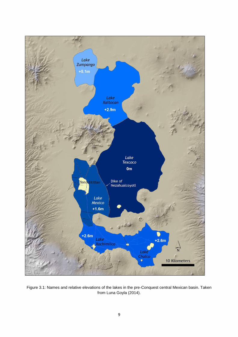
lake Xaltocan (Figure 3.1). The two latter sites are estimated to have covered areas of 9,000-10,000

ha and 5,000 ha, respectively (Crossley, 1999).

Most of the original chinampa fields of the ancient city of Mexico-Tenochtitlán currently lie under the

urban sprawl of the capital, having been partially or completely destroyed, and are only accessible

for study as an adjunct to construction activities. Furthermore, it’s been proposed that the Chinampa

agriculture of the core city served a more supplementary and recreational purpose rather than

intensive food production (Calnek, 1972).

Buried chinampas in the region of Xaltocan to the north have been mapped and are reasonably well

preserved and studied (Morehart, 2016, 2012; Morehart and Frederick, 2014), making them a

reasonably good source of information on pre-modern Chinampa agriculture.

However, while Xaltocan was under Aztec control at the arrival of the Spanish, the area and its

chinampa fields were originally settled by Otomi peoples four to eight centuries before the rise of the

Aztec empire and abandoned at least once in the following centuries (Morehart, 2016), making it

risky to assume methodological and morphological continuity between the chinampas of Xaltocan

and those in the south.

Finally, in portions of what remains of the Xochimilco-Chalco lake numerous chinampas still exist

and a portion of them are still in use. However, Chinampa agriculture in Xochimilco has undoubtedly

been influenced, both physically and culturally, by the deep changes the basin experienced during

the 500 years that followed the Spanish conquest (drainage, deforestation, introduction of European

technologies, change in land use and ultimately urbanization) (Moncada Maya, 1982). This makes

the existing chinampa fields and the current Chinampa tradition less than ideal subjects of study in

the search for an “original” chinampa recipe.

9

Figure 3.1: Names and relative elevations of the lakes in the pre-Conquest central Mexican basin. Taken

from Luna Goyla (2014).

10

From the imperfect nature of archaeological evidence and present-day chinampas follows that any

knowledge derived from physical sources must be complemented with written descriptions and

accounts from pre-modern times. And, since much of the agricultural practice in ancient Mexico

relied on oral tradition, documents from the Spanish Conquest and Colony remain the main source

of information regarding its practices and technology. Unfortunately, these documents are, at best,

accounts written by Conquistadores and Catholic missionaries with no particular aptitude for farming

or natural science. In the words of Wilken (1986), “upon examination it appears that (historical)

descriptions of many, if not most, chinampa structural features are products of casual observation

and speculation rather than careful study and analysis”. Thus, adding written accounts as a source

poses some challenges on its own.

This has indeed led to strangely resilient misunderstandings about the agriculture of ancient Mexico;

for instance, the notion that chinampas were at some point in fact floating gardens, capable of moving

from one place to the other in search for marketplaces or better locations for farming, or to avoid

danger. The idea of buoyant chinampas can be found in accounts from sixteenth-century Jesuit

missionary José de Acosta as well in the records made by 19th century German explorer Alexander

von Humboldt, neither of which were likely to have witnessed a chinampa being built or towed from

one place to another (Crossley, 1999; Wilken, 1986). Even the relatively contemporary Santamaría

(1912) makes reference to this myth, claiming that it was only for the sake of the cadastral record

that most chinampas were anchored and henceforth built so as to stay fixed.

Before moving on, let this particular point be settled: it is nowadays regarded as highly improbable,

if not plainly impossible, that any truly floating chinampas ever existed. Wilken (1986) provides an

exhaustive analysis of the overwhelming physical and logistical obstacles that floating chinampas

would have faced, and makes an excellent point of the purposelessness of attempting such a feat in

the first place. Large barges that served as plant nurseries, on the other hand, did actually exist, and

could be at the root of the misunderstanding (Crossley, 1999; Dunmire, 2004; Wilken, 1986).

Having visited the inherent difficulties in the reconstructing of the “original” Chinampa system from

either physical evidence or written accounts, a natural place to begin doing just that would be the

most widely-accepted existing descriptions of the construction of a chinampa. Here, we will

paraphrase a combination of two very common modern descriptions based on historical sources,

one put together by Wilken (1986) based, among others, on Armillas’ (1971) analysis of 16th and

17th century accounts, and another by Outherbridge in 1987 cited by Frederick (2007):

11

Upon locating a suitable shallow area in the lake, a rectangle was marked with reeds and filled with

layers of interwoven or interbedded aquatic plants, especially tule (most likely Scirpus americanus),

and soil carried from in-land. Upon this foundation, lake mud and soil from older chinampas would

be heaped to a height of approximately 30 cm above the water. Having reached the desired height

and compactness, ahuejote (Salix sp.) trees would be planted along the edges of the newly made

bed at spaces of 4 or 5 meters. The edge could be further reinforced with wooden stakes. The topsoil

would be kept fertile by mixing crushed water plants in it or by spreading a layer of organic-rich lake

sediment before sowing. If a chinampa grew too high above the water, soil could be taken from it to

use in building new ones.

As a contrast, one account from 1599, compiled by Frederick (2007), describes chinampas built

simply by “... carrying in canoes sod (root-rich topsoil) cut in the mainland, to heap it up in shallow

waters thus forming ridges… “. This much simpler description nevertheless implies access to large

amounts of manpower and adequate soil in-land and would result in a mostly monolithic chinampa,

whose pedology would depend on the quality of the terrestrial resources available.

This description, where the raised fields consist mostly of monolithic ridges of moved soil, is however

consistent with the prehistoric ridges found in the Magdalena Valley in Colombia (Parsons, 1986),

and in the highland wetlands of northern Ecuador (Knapp and Denevan, 1986).

A sort of intermediate description from 1723 (Frederick, 2007), involves “heaping sod from land and

mud from the lagoon”, but conspicuously lacks the plant-based foundation of the first description.

Frederick (2007), analysed several historical accounts and compared them to reported and own

archaeological excavations. He identified three broad types of chinampa morphology according to

their internal structure and construction method: 1) massive (monolithic) minimally stratified ridges

often composed of exotic or imported material, corresponding to the simplest method of construction

described above, 2) stratified mounds of thin bedded deposits of organic-rich lacustrine material on

top of a layered foundation of peat, plant material and lake sediment, corresponding to the most

often used description as presented above, and 3) an intermediate between 1) and 2), where layers

of different materials are present, but none is particularly organic-rich and there is no clear evidence

of muck layering on the upper portion or plant material used as foundation.

The resulting soil would be greatly altered by the process of building the fields, regardless of the

specific construction method employed, and thus, it can be considered a man-made soil, or

anthrosol. The source of the material, however, would make a big difference in the characteristics of

a particular chinampa’s soil; fields made mainly from local wetland soils and sediments, would retain

12

many of the properties of a hydric soil, or histosol, like a deep layer with high organic matter contents

(above 20%) and very low bulk density (Brady and Wile, 2008; FAO, n.d.), while fields where most

of the material was imported from the dryland would have more in common with the fertile dark top

layers of a local grassland soil, or mollisol (Brady and Wile, 2008).

Given that no other parameters are explicitly cited, it can be assumed that, even though not included

in the other two descriptions, all these chinampa models are built to roughly the same height and

dimensions as the first description, and are as well supported at the edges by willow trees at similar

intervals.

In order to move forward, let’s assume that the three methods and three corresponding morphologies

describe the range of Chinampa practices one would encounter in premodern central Mexico,

keeping in mind that Frederick (2007) found the morphology fitting most common description (2) to

be the rarest among his study sites, an unsurprising finding if one considers that this description is

the most complex in the spectrum.

As to the dimensions of an individual field, Armillas (1971) cites a 16th century report that states

chinampas were built to be approximately 2.5 to 3.3 meters wide, with no specific limit length-wise.

Furthermore, Frederick (2007) notes that a shift, likely post-Conquest, in chinampa morphology from

around 3 meters of width to around 12 m, with a corresponding shift in land-to-water area ratios from

1:1 to as much as 28:1. Wilken (1986) summarizes the length of chinampas to a range between 10

and 200 meters, while remote sensing mapping using multi-spectral imagery in the buried pre-Aztec

chinampa fields of middle-Postclassic Xaltocan (AD 1200-1400) suggests an average tertiary canal

(the type that separated individual fields) length of just under 50 meters (Morehart, 2012).

The height of a chinampa from the level of the original ground or the bottom of the resulting

surrounding canals is not mentioned in any historical accounts directly or indirectly reviewed here,

as they all describe only the height above the water level after construction. Armillas (1971) places

the maximum lake height near Xochimilco at 2238.8 masl and a plant-based foundation 40 cm below

it. Counting on a plant mat thickness of 40 to 60 cm for the foundation (Wilken, 1986), this would

place the original ground level at about 80 cm to 1 m below the maximum lake stage. As mentioned

before, the most popular descriptions of Chinampa systems put the surface of an active chinampa

at 30 cm above the water level, thus making the total height of piled material about 110-130 cm.

However, Wilken (1986) challenges the notion of such low-lying surfaces arguing that the risk of

waterlogging (and flooding) during rain seasons would have encouraged prehispanic farmers to build

their fields higher above the water level, in the order of 80 to 120 cm above canal levels, resulting in

a total height of moved earth of 1.5 to 2 m. Indeed, some sources quote heights above the water of

13

“no more than a few feet”, “less than a vara (84 cm)” and “nearly a meter” (Armillas, 1971; Wilken,

1986).

It is possible to conciliate these seemingly conflicting accounts if the water level is allowed to change

in time, the different versions corresponding to different seasons or years. Robertson (1983)

modelled the variations in the pre-Conquest lake’s water levels in years of normal, high and low

precipitation, both in a completely natural state and in a controlled state reconstructed from available

accounts of late Aztec hydrological engineering. He estimated that, as a result of strongly seasonal

rains and the shallow shape of the basin, water levels around Xochimilco varied over 50 and as

much as 70 cm in normal years if no hydrological controls were in place, with extreme years seeing

variations well over 1 meter. Thus, if 30 cm was the height of the chinampas at the maximum stage

of the lake on a normal year, a height of 1.3 m above the original ground would see a chinampa with

at least 30 cm of standing water around it at the minimum stage, enough for bucket irrigation and

careful canoe transit. The canals would only dry or the fields flood following years of extreme-low or

high precipitation, respectively. This variation, and the risk that came with it, would have been greatly

reduced via water control systems built by the expanding Aztec empire (Robertson, 1983).

Whether chinampas were built on actual aquatic beds (where there is permanently standing water

over the sediment) or on more marshy areas, is also a debatable point. The interesting

misunderstanding of chinampas as “floating gardens” does tell us that foreigners observing

Chinampa agriculture after the conquest generally saw standing water around them. Armillas (1971),

on the other hand, estimates based on excavations near Xochimilco that Chinampa agriculture (in

the Xochimilco-Chalco lake, at least) was established on “what was swampy ground at the end of

dry seasons”. How to interpret the word “swampy” in this description is somewhat problematic, but

modern wetland classifications generally define a swamp as “a wetland dominated by woody

vegetation (trees and/or shrubs) that is flooded for variable periods during the growing season”,

which implies that the original ground is not under permanently standing water (Tiner and Burton,

2009). Accepting this definition would mean that the resulting canals that surrounded the Chinampas

would only actually be permanently covered with standing water after the chinampa had been built

and the surrounding canals dug sufficiently deep.

However, it is quite possible that chinampas were built in both wetter and dryer grounds depending

on local space and material resources. It could be ventured, from the varying construction methods

known so far, that foundations and interbedding made from plant material correspond to chinampas

built in areas of permanently standing water to assist in the first stages of chinampa construction,

14

while in seasonally or temporarily dry grounds the simpler method of monolithic construction with

ditches dug into the original ground to make canals would have been preferred.

Let us, then, consider a model chinampa constructed in shallow standing water: 3 m wide, 50 m long

and 1.3 m high starting at the original ground level, where the top 30 cm of soil is permanently above

the water and regularly amended, the 70 cm below are seasonally or intermittently saturated and the

bottom 30 cm are permanently inundated. This chinampa would have an area of 150 m2 (or 0.015

ha), a total volume of 195 m3 and a dry mass of 78 tons given a bulk density of 0.4 ton/m3

corresponding to the upper bounds of relevant organic soils (Krasilnikov et al., 2011)(Crossley (1999)

puts the bulk density of fresh muck at 0.42 ton/m3). About 45 m3 or 18 tons of chinampa material

would be permanently above the water, while the same amount would be permanently inundated.

105 m3 or 42 tons of chinampa soil would thus be intermittently or seasonally saturated. While the

practice of almárcigo, a bed filled with muck and used as a nursery for sapling plugs, is not

considered in this model chinampa, the practice of amending all productive soil with a thin layer of

muck is. This layer will, in our model, consist of fresh superficial muck or lake sediment, 5 cm thick,

added before each sowing to boost soil fertility. Finally, there would be Salix bonplandiana (named

ahuejote in most of central Mexico), a species native to and common in Mexico, planted along the

edges of the long sides at 5 m intervals, to a total of 20 trees per chinampa.

3.2 Carbon pools and fluxes

With the previous considerations in mind, we can begin to work out an ecosystem ecology for a

generalized, inferred form of the premodern fields, beginning with the backbone of any ecosystem

in terms of energy and biomass: carbon.

Carbon is the main energy currency in practically every ecosystem, as well as the main structural

element of all living organisms. Carbon is also the defining constituent of organic matter in soils and

sediments (soil organic matter, or SOM). As materials from different sources have different relative

carbon contents, different chinampa constructions would lead to different pool sizes in the soil, and

different management methods would result in different fluxes between the atmosphere, lake, soil

and the local community. Thus, the location of a particular chinampa, as well as the construction

method used, would have a great influence on the internal composition of a chinampa and the size

of its initial carbon pool.

The material in monolithic chinampas would have similar carbon contents as the soils or sediments

they were built from, ranging anywhere from the 1% carbon of local modern haplustolls under

cultivation (carbon contents of local prehispanic dryland soils could not be located) (Dendooven et

15

al., 2012; Ortiz-Cornejo et al., 2015; Patiño-Zúñiga et al., 2009) to over 20% organic matter as

expected in hydric soils (histosols) and mucky wetland sediments (FAO, n.d.). A particular field’s

position in this spectrum would depend on the origin of the material used in its construction, whether

it was wetland soil simply moved on-site, or it was imported from nearby dryland. Given the large

workforce required to move large amounts of soil (without domestic animals or machinery) from the

dryland in to the marshy edges of the prehispanic lakes, let’s assume that whenever possible,

monolithic chinampas were built from exposed marshy histosols, a reasonable proposal considering

that the material from digging ditches to form canals could be used in the chinampa itself. Given that

the carbon content of the wetland muck available for chinampa construction likely varied depending

on local conditions such as the hydric regime, we will use the minimum defining SOM content of a

histosol (20% SOM, corresponding to 10% carbon) as a catch-all estimate for the structural

components of a chinampa composed of local wetland muck.

Chinampas built after the more complex model of layered plants and muck would tend to include

layers with higher carbon contents, starting at the carbon content of the local muck (10-25%) and up

to around 40% in the layers composed primarily of green plant material (Brady and Wile, 2008). The

chinampa profile in Mixquic reported by Parsons (Parsons et al., 1986) fits just this description, with

layers corresponding to the base about 40 cm thick and rich in uncharred plant material.

Using the model chinampa from before, a monolithic construction would result in an initial pool of

carbon of at least 7.8 ton-C if built from a marshy histosol with 10% organic carbon, as we’ve chosen

to assume. By area this figure can be normalized to 520 ton-C/ha.

A more complex chinampa, with a 40 cm-thick foundational plant mat and a body composed primarily

of local histosols with some interlayed plant material would present a larger initial carbon pool. If the

foundation is primarily plant material built to barely emerge from the water, as can be interpreted

from historical accounts, a 30 cm-thick layer with a dry weight carbon concentration of 40% is

reasonable, making up a permanently inundated pool of 7.2 ton-C, four times the size of the

permanently inundated portion of the monolithic construction. The overlaying 1 m of soil would have

a slightly higher carbon content than the lake muck itself, depending on the amount of plant material

interlayed in it, but if consisting primarily of muck it would at least contain 20% SOM. This yields a

carbon pool of 6 ton-C, which leads to a total initial chinampa pool of 13.2 ton-C. This value

normalized by area is equal to 880 ton-C/ha.

The starting pools from chinampas built within the spectrum of construction methods between

massive (monolithic) and highly stratified, would likely fall between the two values just calculated.

16

However, both the portion of the chinampa permanently raised above the water and the portion

seasonally or intermittently saturated would be subject to significant respiration and lose some of

their carbon to the atmosphere. The permanently inundated portion of the chinampa (bottom 30 cm),

on the other hand, would likely retain its original composition for a good deal longer, particularly if

one assumes any pre-existing wetland soil to be close to equilibrium in its environment. Thus, this

portion of a chinampa constitutes a pool of 1.8 ton-C (120 ton-C/ha) if made from wetland material,

and 7.2 ton-C (480 ton-C/ha) if made of plant material.

Wilken (1986) mentions an organic matter content of 17% in prehispanic chinampa soils, which

translates into an organic carbon content of 8.5%. This is high for a soil, but lower than what we

suppose for the original material. Since the lower portions of the main bulk of the chinampa would

remain inundated for longer (assuming a gradual rise and fall of the lake stage throughout the year),

decomposition would occur more slowly deeper within the chinampa. If we set the boundary between

the permanently inundated material and the intermittently/seasonally saturated material at the

estimated value of 10% carbon, and the upper boundary of the periodically saturated soil at the 8.5%

carbon value mentioned before, an initial approximation would put the average carbon content in

this region at 9.25% by dry weight. This gives a pool of 3.89 ton-C in our model chinampa, to an area

value of 259 ton-C/ha.

In the permanently aerated portion of the chinampa we can imagine a similar gradient to the one

formed in the periodically saturated bulk. Respiration can reasonably be expected to be fastest at

the upper part of the soil and slowest near the upper limit of the lake stage. However, amendments

would also be added at the surface, and they famously consisted primarily of organic-rich lake

sediment. Remembering this, and that the technique of ploughing or turning the soil was first

introduced by the Spanish after the conquest, a sufficiently diligent farmer could turn the gradient

around to the point where the topmost soil approached the carbon content of fresh rich muck and

the slow downwards movement of dissolved and particulate carbon allowed bottom of the topsoil to

be in equilibrium with the topmost part of the periodically saturated bulk. This last supposition may

seem strange, but will later prove not to be entirely unfounded.

Robertson (1983) mentions organic matter content in chinampa sediment samples extracted from

under permanently standing water of up to 60%, i.e. 30% carbon. Crossely (1999) similarly states

that the organic content of canal sediment is twice that of most chinampa topsoils. If we assume this

is upper limit is the carbon content of the prime newly-formed lake sediment that Chinampa farmers

looked for to use as amendment (human manure has a slightly lower but similar carbon content)

(Rose et al., 2015) we can assign this carbon content to the upper surface of a well- maintained

17

chinampa soil. The lower boundary of the permanently aerated soil, being in equilibrium with the soil

on the opposite side of the boundary, would then have a carbon content of 8.5%. We can then

estimate an average carbon content in the upper 30 cm of the chinampa of 19.5%, giving us a pool

3.51 ton-C (234 ton-C/ha).

The previous adds to a theoretical estimate of the total carbon pool within a living chinampa of 9.2

ton-C (613 ton-C/ha) for monolithic constructions and 14.6 ton-C (973 ton-C/ha) for chinampas with

a plant-based foundation.

This indicates a potential general net sink of around 93 ton-C/ha from transforming the terrain into

an active chinampa, supposing that the sediment used as amendment would otherwise have

remained unoxidized in the bottom of the lake. This sink would have been expanded by permanent

vegetation on the chinampa, particularly the ahuejote (Salix bonplandiana) trees planted on its

perimeter. Specific biomass calculations for this species in the Central Basin of Mexico could not be

found, but ahuejote trees are known reach 6 to 10 meters in height and measure up to 80 cm in

diameter at chest height, so a permanent biomass pool of 400 kg per tree, 4 ton per chinampa,

seems reasonable (Salix bonplandiana, 2018). This means an intermediately long-term carbon pool

of about 2 ton-C per chinampa, or 133 ton-C/ha in tree biomass, with an estimated turnover of 20 to

30 years (Salix bonplandiana Kunth, 2012). Supposing the trees are replaced quickly enough after

the end of their lives, this pool can be considered permanent in the chinampa, although it can be

argued that the final use of the wood from old trees can greatly influence the general carbon flow of

the Chinampa landscape.

Having outlined the general long-term carbon pools in the Chinampa system, it is necessary to look

at the main flows influencing an established chinampa. The staple flow of this system is the mucking

with rich sediment dragged from the lake bottom and spread over the surface before sowing (or

introducing plugs with seedlings, if these were grown elsewhere). As argued before, archaeological

evidence suggests this material was very high in organic carbon, and finding prime spots for mucking

before sowing must have been an important part of the agricultural technique. This also sets the

muck used as amendment apart from the muck/histosol used as a structural component of the

chinampa, the former being likely more superficial, recently deposited detritus that has not had time

to decompose much. Counting on two harvests of maize per year, this would mean two 5-cm layers

of muck per year, or 15 m3 of carbon-rich muck (bulk density 0.4 ton/m3 and 30% carbon by mass),

representing a flow of 1.8 ton-C per chinampa, or 120 ton-C/ha*yr. Ergo, given an original land-to-

water area ratio of 1:1 in the pre-Conquest Chinampa fields, the same 120 ton-C/ha*yr would have

needed to be deposited upon the bottom of the canals, implying a net primary productivity at least

18

as large in the water column. This quantity is at least ten times larger than the net primary productivity

in a fertile subtropical wooded wetland (Brinson et al., 1981), and as such makes it unsustainable to

source the muck from the canals between the chinampas themselves. In the premodern lakes,

however, it is possible this wasn’t a prohibitive problem, as the portion of the lakes actually turned to

agricultural land was still much smaller than that of the lakes and surrounding wetlands themselves.

Luna Goyla (2014) puts the area of the high water level lake at the time of the Spanish’s arrival at

around 1,000 km2 (100,000 ha), while the total cultivated area occupied by chinampas at between

6,000 and 9,000 hectares. Even with this nearly 10:1 abundance of aquatic versus chinampa

environment, overexploitation of fresh muck could have become a critical weakness of the Chinampa

system.

Crossley (1999), reflects on this point and the apparent unsustainability of mucking for every sowing,

and proposes that mucking occurred more infrequently, only when the soil became impoverished.

Halving the mucking frequency to only once a year would lighten the load on the muck sources to

only 60 t-C/ha*yr, still well beyond the primary productivity of the aquatic environment. A much lower

frequency, less than once every five years, would be needed to match the muck requirements to an

NPP of 1000 g-C/m2*yr in the aquatic environment.

While studying the Ecuadorian relatives of the Chinampa raised fields, Knapp & Denevan (1986)

argue that while muck is a rich source of nitrogen, the pre-Inca dwellers that worked in them likely

supplemented the phosphorus in fields using human manure. This supposition has also been made

in the context of Mexican chinampas by both Wilkes (1986) and Robertson (1983). Parsons

calculated that a single family had access to 1100 kg (dry weight) of human and small animal waste

per year. Morehart (2016), on the other hand, calculates that a single adult farmer could take care

of 0.7 ha on his own in the pre-Aztec chinampas of Xaltocan. Assuming simple small nuclear families

(capable of caring for 1 ha per family unit), these two figures can be combined to estimate a flow

onto the soil of about 1 ton of human waste per hectare per year, i.e. an additional 0.5 ton-C/ha*yr.

Using human and small animal manure would likely have been a mix of an intrinsic flow, where

carbon added to the soil comes from the portion of the harvest that the family itself consumed, and

extrinsic, where the family exchanged or otherwise acquired food from outside the field and thus

added carbon to the soil besides that from in-situ primary production. Morehart (2016), however,

calculates that chinampa farmers in the region would’ve had over 90% of their harvest as surplus

after feeding themselves and their families, and thus this flux can safely be assumed to be entirely

intrinsic, that is, a return to the soil from the field’s NPP.

19

Being surrounded by standing water in a wetland environment, carrying plant waste away from a

chinampa would’ve been highly impractical, so it is natural to assume that this too was primarily

composted in situ. This represents a return flow of carbon (as well as other elements) from harvest

activities. The amount of carbon thus retained by composting plant waste would depend on the net

primary production of the crops grown on the soil, the proportion of the plant actually consumed or

otherwise utilized by humans, and the amount of carbon lost to respiration during the composting

process.

An approximation can be made using a common estimate of Chinampa maize productivity proposed

by Sanders as cited in harvest surplus calculations by Morehart (2016) in pre-Aztec Xaltocan calorie

surplus, and by Luna Goyla (2014) in the late 15th century lakes of Xochimilco and Chalco. This

estimate puts maize productivity in premodern chinampas at 3,000 kg of maize grain per hectare per

year. Maize has been intentionally bred for millennia in the American continent before the Spanish

Conquest or modernity and thus it seems safe to use a harvest index of 0.45 (HI = grain yield/plant

biomass), the same as modern pre-1930’s North American cultivars (Hay, 1995). This turns the

3,000 kg/ha*yr of grain into a total yearly above-ground biomass productivity of 6,666 kg per hectare.

With a 43% carbon content in dry matter and an average water content at late dough stage of 71.4%

(Latshaw and Miller, 1924) this is equal to an above-ground NPP of 830 kg-C/ha*yr.

However, Chinampa agriculture is intrinsically a polyculture that combines different cash crops with

support and wild plant species. Therefore, it is also important to estimate the total and above-ground

primary productivity in the chinampa environment. These quantities can be estimated thanks to the

fact that water is a stoichiometric component of photosynthesis, and in general an important part of

plant metabolism. Therefore, although the relationship is complex and varies between climatic

regions and plant communities, relatively simple functions between water used by plants and the

carbon fixed by them can be inferred from empirical data. The factor relating plant growth in terms

of carbon fixation to water use is commonly termed water use efficiency (WUE), and a number of

models have been constructed in recent decades that aim at accounting carbon budgets in scales,

places and times inaccessible for direct measurement. These models normally use either plant

transpiration or the evapotranspiration of a particular soil with plant cover, and relate it to either gross

or net primary production (GPP or NPP). Other similar models relate GPP and NPP to precipitation

and temperature, both of which are intimately related to both transpiration and evapotranspiration.

All these models make generalizations and assumptions and thus carry uncertainties, but altogether

represent the best option for estimating vegetation growth in the ancient Chinampa agricultural

system (See equations 3.1a and 3.1b).

20

(3.1𝑎) 𝑊𝑈𝐸𝐸𝑇 = 𝑁𝑃𝑃𝐸𝑇⁄ ; (3.1𝑏) 𝑊𝑈𝐸𝑀𝐴𝑃 = 𝑁𝑃𝑃

𝑀𝐴𝑃⁄

Equations 3.1a and 3.1b. Water use efficiency (WUE) as a function of net primary production (NPP) and evapotranspiration (ET) (1a), and as a function of NPP and mean annual precipitation (MAP) (1b). Given

know WUE and ET or MAP, NPP can be calculated.

Robertson (1983), in modelling the pre-Columbian hydrology of the central Mexican basin, calculated

the yearly precipitation and potential evapotranspiration (PET) in agricultural land around the late

16th century lakes of Chalco, Xochimilco and Mexico (referring to the part of the Texcoco lake where

the ancient city of Mexico was built, later enclosed by hydraulic control structures). He reports a

mean annual precipitation in the range of 534 to 799 mm, and potential evapotranspiration in the

range of 449 to 463 mm.

Potential evapotranspiration is not necessarily equivalent to actual evapotranspiration (AET), the

parameter most often used in WUE calculations, but If we consider, in accordance with the

Chinampa paradigm, a diligent Chinampa farmer keeping year-round plant cover and a field where

all of the plants’ hydric requirements are met, we can assume that PET is very close or equal to AET.

Thus, using WUE values reported by Ito & Inatomi (2012) for cropland (0.85 and 2.07 g-C/kg-water

for NPP and GPP respectively), one hectare of chinampa soil would see a yearly NPP of 3.81-3.93

ton-C and a GPP of 9.29-9.58 ton-C. These values are similar to those obtained using the lower-

bound WUE for cropland obtained by Beer (2009, cited by Ito & Inatomi, 2012) of 1.57, which yields

a yearly GPP of 7.05-7.15 ton-C/ha.

On the other hand, calculating above-ground and total NPP from mean annual precipitation (MAP)

using the model for non-tree dominated biomes by Del Grosso (2008), yields values of total net

primary production (TNPP) = 2.1-3.1 ton-C/ha*yr and aboveground primary production (ANPP) =

1.0-1.5 ton-C/ha*yr. Knowing that one of the core paradigms of Chinampa agriculture is that of

independence from rain, these values probably don’t describe our case as well as those derived

from potential evapotranspiration. However, they do offer a general notion of the proportion between

above-ground and total net primary production in non-tree dominated biomes, a value that we can

apply to figures derived via other methods.

The Salix trees that surround the chinampa will be considered apart from the crops and plants grown

in most of its soil since they do not seem to be cut to any degree during their life. They did

undoubtedly form part of the local hydrology, so they need to be accounted for in the primary

production. According to modern forestry records, the total NPP of Salix bonplandiana in Mexico falls

between 307 - 793 g/m2*yr, which, if we concede one square meter of the chinampa per tree, at a

21

rate of 20 trees per chinampa corresponds to a net productivity of 400 and 1000 kg-C/ha*yr (Salix

bonplandiana, 2018). Excluding, then, the net productivity of the ahuejote trees from the NPP derived

from evapotranspiration, the result is a crop-NPP of 2.87 - 3.40 ton-C/ha*yr.

If we then apply the ration of ANPP to total TNPP by Del Grosso, we obtain a crop ANPP estimate

of 1.38 - 1.64 ton-C/ha*yr independent of precipitation. Of this aboveground productivity, 0.56 - 0.81

ton-c/ha*yr would belong to plants other than maize or ahuejote trees.

The difference between the aboveground NPP derived from caloric calculations for Xaltocan and the

aboveground NPP calculated from evapotranspiration is an amount not easily overlooked. This

difference could be due to overly modest estimates of chinampa maize yield, or rather reflect the

complementary part of Chinampa polyculture that cannot be accounted for only with maize yields,

even though maize was the main calorie source of the time. Other crops, mainly amaranth, beans,

tomatoes and gourds, would’ve been grown together or rotated with maize for consumption, while a

variety of herbs, chili peppers and roots would’ve complemented the harvest (Dunmire, 2004). The

sheer diversity of the crops grown on a chinampa makes the task of calculating the exact portion of

the soil’s productivity that was used for human consumption impractical, so an approximation will be

made. Modern varieties of beans grown in Mexico have a harvest index of 0.54 (Berrocal-Ibarra et

al., 2002), while Cucurbita pepo Linn, an heirloom gourd known to be domesticated in prehistoric

Mexico (“Cucurbita pepo Linn. [family CUCURBITACEAE],” 2018), has a harvest index of 0.52 when

properly irrigated (Fandika et al., 2011). Thus, to be on the safe side, it will be assumed that in

general 50% of the remaining above-ground plant mass was consumed or utilized in some manner,

and thus removed from the system, while the remaining 50% was composted on-site. This yields a

removal of non-maize, non-perennial plant carbon of 0.28 - 0.40 ton-C/yr*ha, and an equal amount

of compost. For the maize crops, the 3,000 kg/ha*yr of grain removed from the field translate into

0.37 ton-C/ha*yr, leaving behind 0.46 ton-C/ha*yr for compost.

No specific estimations of respiration rates from maize-bean-squash litter in premodern composts

could be located, so we will estimate that 50% of the carbon in the plant litter is lost to heterotrophic

respiration during a year of composting (Brady and Wile, 2008). Thus, of the 0.74 - 0.86 ton-C/ha*yr

removed from the soil but not consumed (both maize and not-maize ANPP), the amount of carbon

returned to the soil as part of soil amendment is 0.37 - 0.43 ton-C/ha*yr.

The specific premodern technique for removing plants at harvest is not mentioned in any of the

literature thus far reviewed, but for simplicity we will suppose that no particular effort was put in the

removal of root mass beyond simply pulling out the plant from the soil. Thus, we’ll assume that all

below-ground carbon fixed by primary production remained in the soil and took part in the trophic

22

pathways of detritivores and microorganisms. This fraction of the total NPP has a magnitude of 1.49

to 1.76 ton-C/ha*yr.

Together with the carbon influx from soil amendments (mucking, manuring and addition of compost),

carbon built up from below-ground NPP would be subject to respiration. This process would be

considerably slower than in modern agriculture due to the absence of the plough in pre-Conquest

times, but other than that there is no real information on actual 15th century soil respiration rates.

Using modern data from unamended chinampa soils from Xochimilco, we can estimate such fluxes

to be between 1.50 and 1.65 ton-C/ha*yr (Ortiz-Cornejo et al., 2015). It is difficult to gauge what

effect would constant mucking have on the respiration rate of a chinampa soil, and unfortunately, no

experiment explicitly involving mucked soils has been found, so without evidence to the contrary a

yearly carbon outflow of 0.55 - 0.6 ton-C/ha will be used.

The full carbon network described above is summarized in Figure 3.2. It should be quickly evident

that mucking before every sowing is as much a massive input of carbon to the Chinampa soil system,

as it is potentially critically depleting for the aquatic environment, and it would accumulate organic

carbon at a rate that soil respiration couldn’t possibly keep up with. If mucking is a vital input of

nutrients as some sources make it out to be, then the Chinampa system as previously outlined would

have depleted its surrounding carbon resources ten times faster than they could replenish

themselves, and would thus have relied on centuries of previous carbon deposition in the wetland

soil. As mentioned before, mucking before every sowing could be a large overestimation of the actual

frequency of this practice, and it would make much more sense that it was used as a sort or new soil

layer, to be laid on top of an exhausted topsoil. How often this was necessary would have depended

on how effectively the farmer amended the soil through the use of manure and compost, and in the

quality of the chinampa’s original material. However, if he could manage to only lay a new layer of

muck once every five years, approximating a the net primary production in a healthy wetland

environment, the yearly input to the chinampa soil would fall to 12 ton-C/ha*yr, still surpassing NPP

by nearly a factor of three.

A final carbon balance in this system can be calculated as shown in Equation 3.2 and Table 3.1.

(3.2) 𝑁𝑃𝑃 + 𝑀𝑢𝑐𝑘𝑖𝑛𝑔 + 𝐻𝑢𝑚𝑎𝑛 𝑀𝑎𝑛𝑢𝑟𝑒 − 𝐻𝑎𝑟𝑣𝑒𝑠𝑡 − 𝐿𝑖𝑡𝑡𝑒𝑟 𝑅𝑒𝑠𝑝. − 𝑆𝑜𝑖𝑙 𝑅𝑒𝑠𝑝. = ∆𝐶

Equation 3.2. Carbon balance in the premodern Chinampa system.

This equation yields, using a mucking frequency of once every five years, a total net accumulation

of 13.58 - 13.79 ton-C/ha*yr. Even discounting the input from mucking, the balance is a net

accumulation of 1.58 - 1.79 ton-C/ha*yr. Further discounting the 1 ton-C per hectare per year taken

23

up by the ahuejote trees that lined the fields, leaves a positive theoretical net balance in the soil of

0.58 - 1.79 ton-C/ha*yr, which would be comprised of plant litter and root mass which would slowly

get integrated into the soil.

Table 3.1. Carbon budget of the theoretical premodern chinampa soil. All fluxes are in units of ton-C/ha*yr.

Flux IN OUT

NPP 3.81 3.93

Mucking 12

Manure 0.5

Maize harvest 0.37

Non-maize harvest 0.28 0.40

Litter (compost) resp. 0.37 0.43

Soil resp. 1.50 1.65

Budget

(In - Out)

Low values High values

13.79 13.58

24

Figure 3.2: The theoretical ecosystem ecology of carbon in a 15th-century chinampa. Pool sizes are indicated in white with units of ton-C/ha. Fluxes and flux sizes for are indicated in black with units of ton-

C/ha*yr.

Naturally, these fluxes would be complemented by the slower losses from the continued oxidation of

the intermittently submerged and permanently saturated portions of the chinampa. Whether the

accumulation from the top was large enough to still make the Chinampa system a net sink in the

longer term, and whether the downwards motion of dissolved and particulate carbon was significant

enough to alter the carbon profile of the chinampa soil, or even the carbon balance of the surrounding

water is unfortunately beyond the capacity of this thesis to estimate, having already taken great leaps

of faith in the construction of this rudimentary, and very general, Chinampa ecosystem ecology of

carbon.

25

3.3 Nitrogen pools and fluxes

Nitrogen is often the limiting nutrient in agricultural systems, and it is absolutely necessary for proper

plant growth. The movement of nitrogen through an ecosystem, however, is different from that of

carbon. Fixation of nitrogen from the atmosphere, while a vital process in many ecosystems, can be

very slow or non-existent in others. And while there can be important losses of nitrogen to the

atmosphere through denitrification and anaerobic ammonium oxidation, these processes are

performed by microbes, and occur separate from the plants and animals that are the focus in an

agricultural system’s biomass.

The initial size of the long-term nitrogen pools in a chinampa would be closely related to the nitrogen

content of the parent materials, i.e. wetland mucks and, in some cases, dryland topsoils. Since

nitrogen is rarely included in their analyses, archaeological explorations are of little value when

estimating premodern nitrogen content of the ancient wetland soil; therefore, modern figures will be

used in our model chinampa. It is, however, vital to keep in mind that the 20th century saw a dramatic

change in global and local nitrogen cycles, particularly due to the development of the Haber-Bosch

process and the expansion of both agriculture and urban sprawls (Erisman et al., 2008), and as such

contemporary values might not be representative of the premodern environment.

Regardless, based on modern values, with a total mass of 78 ton, a monolithic chinampa made

entirely of a nearby dryland haplustoll with a nitrogen content of 1.2 kg-N/ton (Patiño-Zúñiga et al.,

2009) would correspond to a starting nitrogen pool of 0.094 ton-N per chinampa, or 6.24 ton-N/ha.

A monolithic chinampa made from wetland soil, on the other hand, with the total nitrogen content of

5.8 kg-N/ton found at 30-60 cm of depth in present-day Xochimilco (Ibarra, 2010) would make up an

initial nitrogen pool of 0.45 ton- per chinampa or 30.16 ton-N/ha.

Finally, a foundation of plant material would represent an initial repository of 0.271 ton-N per

chinampa, or 18.1 ton-N/ha, using a plant biomass nitrogen concentration of 15.081 g-N/kg, as

measured in a Scirpus-Equisetum temperate wetland (Auclair, 1979). The rest of such a chinampa

could be assumed to have the same initial N concentration as local wetland soil, giving a total starting

nitrogen pool of 0.62 ton-N per chinampa, or 41.3 ton-N/ha.

Like the initial nitrogen pools, knowledge about most of the processes involved in the 15th-century

nitrogen fluxes is scanty at best, particularly for the processes that occurred in the long-gone lake

environment, but some approximations can be made based on historical accounts and modern data.

Mucking being a staple mass flow in Chinampa agriculture, it is arguably the first flow worth

quantifying in our model. Unfortunately, the biogeochemistry of the bottom of the 15th century lakes

26

is nowadays completely lost to us, as are the exact macroscopic properties of the sediment selected

by the original Chinampa farmers for mucking. In analysing modern Ecuadorian raised field

agriculture, Knapp (1986) estimates that such a field would require 50 kg-N/ha*yr for sustained high

yields. Given the titular role given by many sources to mucking as a nutrient source for Chinampa

agriculture, we’ll use this 50 kg-N/ha*yr figure as its corresponding nitrogen flow. With a yearly fresh

sediment input of 1.5 m3, corresponding to adding one 5 cm layer on the entire chinampa’s surface

every five years, and a density of 0.4 ton/m3, such a flux would put the nitrogen concentration of

choice lake sediment at 0.125%.

Naturally, the nitrogen flux described above would have actually been a pulse five times larger one

year followed by a decomposition process that by no means can be thought to be constant over the

following four years. Unfortunately, a more temporally-detailed description is beyond the capabilities

of this model.

The assumption made in many historical and older modern descriptions of Chinampa agriculture,

that mucking provided most of the necessary nutrients for sustained high yields, implies that the

supply of nitrogen to the soil depended on the rate of nitrogen fixation in the water and the efficiency

in which nitrogen is cycled between the soil and the water column.

Nitrogen fixation in lake environments can vary greatly with a number of ecosystem parameters like

micronutrient concentrations in the water and amount of sunlight, but the macronutrient regime in

the water is arguably the most important when estimating fixation rates. Oligotrophic lakes

experience very low, sometimes nil, rates of nitrogen fixation, while eutrophic lakes can reach rates

of up to 10 g-N/m2*yr, or 100 kg-N/ha*yr (Burton and Tiner, 2009) and maintain concentrations of up

to 10 mg-N/l (Vasey, 1986). No direct analysis exists of the nutrient regime in the ancient central

Mexican lakes, but one observation made by Hernán Cortéz (leader of the Conquistador army that

brought down the Aztec capital of Mexico-Tenochtitlán) can provide a clue. He observed that in the

indigenous people consumed a sort of “scum, neither plant nor soil” which they gathered with nets

from the lake surface at certain times of the year (Dunmire, 2004). This material, actually a

cyanobacterium that bloomed seasonally (Farrar, 1966), was dried in the sun and eaten much like

Europeans ate cheese, and, according to Cortez, was delicious in a spicy chili dish. The culinary

properties of this scum notwithstanding, it points at a rather eutrophic, if unpolluted, lake with regular

massive blooms of nitrogen-fixing microbiota. How much of the eutrophic regime in the 15th century

lakes was a consequence of human activity, chiefly agriculture, is yet another interesting unknown

in the Chinampa system. Nevertheless, lacking site- and time-specific data, the aforementioned high

values of nitrogen fixation rates and water nitrogen content will be used in our model chinampa.

27

Besides mucking, the use of human manure would have been another important input of nitrogen

into the soil. Knapp & Denevan (1986) estimates, as mentioned before, that a family of farmers would

be able to produce about one tonne of human and small animal manure per year, a figure we can

round up to 1,000 kg/ha*yr, and which corresponds to 30 kg-N/ha*yr. It is difficult to estimate the

exact degree to which a farmer family would consume products traded from outside their own

chinampa, as it likely depended greatly on the family’s geographic and socio-political situation.

Therefore, and for the sake of simplicity, this flow will be considered as entirely extrinsic.

An unexpected input of nitrogen on the soil could have been canal water. Vasey (1986) studied the

difference in biomass of maize at the time of silking between plants watered with tap water and plants

watered with algae-rich canal water in a controlled N-limited island bed (raised bed with permanently

or seasonally standing water around it) environment. Maize grown using canal water had similar

biomass to that grown with a standard urea solution, significantly higher than maize grown with tap

water. Direct use of nitrogen from the canals by roots extending down, however, was found not to

play a significant role in crop growth, likely because microfauna was much faster at taking up nitrogen

in saturated soil and standing water than the reaching roots of plants.

This implies that nitrogen, both organic and inorganic, could flow from the canals into the soil via

surface irrigation in locations where the water table was seasonally low, a situation that can be fitted

into our chinampa model. According to Vasey, with a monthly watering rate of 200 mm per month

six months per year a raised bed soil would receive 12 kg-N/ha for every milligram of nitrogen per

litre found in the canal waters. In our chinampa, the percentage of the year where irrigation with

canals water would be necessary corresponds to the amount of time the water stage is further from

the surface than the height of capillary rise in the soil, a length of time that can be approximated

assuming a sinusoidal vertical movement of the lake stage. The total amount of water supplied from

the canals would then be equal to the same percentage of the annual evapotranspiration as the

percentage of the year that the lake stage is too low for capillary rise to reach the surface. Wilken

(1986) places the range of height in capillary rise between 40 and 120 cm for most agricultural soils,

from which we’ll pick a conservative value of 60 cm. This puts the number of days where bucket

irrigation is necessary, that is, the number of days in which the lake stage is lower than 60 cm from

the surface, at roughly 90 days per year, or 25% of the year. Thus, using Robertson’s

evapotranspiration figure of 455 to 463 mm/yr, the volume of water carried from the canals every

year falls to roughly 17,000 litres per year per chinampa field. This, in turn, means a yearly flow of

nitrogen of 11.3 kg-N/ha if we suppose an average nitrogen content in water of 10 mg-N/l.

28

One more possible flow of nitrogen from the water environment into the soil is from water plants

added into it as green manure. The reason this activity hasn’t been taken into consideration until

now is that it is very difficult to estimate its extent and precise nature from historical sources. Some

accounts compiled in the 20th century mention the use of crushed water hyacinths to increase the

fertility of the soil in pre-Conquest or early Colony chinampas (Crossley, 1999). However, the water

hyacinth (Eichhornia crassipes), native to the Amazon river basin, was first introduced in central

Mexico in the 1890’s (Crossley, 1999; Miranda A and Lot H, 1999). Robertson (1983) mentions

duckweeds as a potential native source of green manure with a dry mass nitrogen content of up to

7%, but recognizes that it is unknown whether the ancient Aztecs took advantage of such resource.

Returning to the previously used value for the nitrogen content in plant material from a Scirpus-

Equisetum wetland (Auclair, 1979), we can estimate that a farmer would add 15 g of nitrogen to the

topsoil for every kilogram of plant material he added to it. The actual amount added would have

varied depending on the farmer’s individual judgement, his success in finding and transporting muck,

and the availability of plant litter compost and manure.

Finally, symbiotic nitrogen fixation in soil could have played an important role in the agricultural

ecosystem of the time. According to Jiménez-Osornio & Gómez-Pompa (1991), the main five native

crops of central Mexico were maize, beans, squash (or a related gourd), amaranth and chia. Of

these, particularly beans and squash are thought to be traditionally grown simultaneously to maize

as an intercropping triad (Santillán, 2014) so for now we’ll leave the chia and amaranth crops out of

our model. Beans are of importance for the nitrogen cycle because they are good nitrogen fixers,

with symbiotic biological nitrogen fixation (BNF) rates of 30 - 50 kg-N/ha*yr (Brady and Wile, 2008).

Due to the practice of intercropping, the density of bean plants was likely lower in Chinampa

agriculture than in the studies from which this range of BNF was derived. For that reason, we’ll

choose to use the lower-bound value of 30 kg-N/ha*yr for our model.

The main outflows of nitrogen from the soil would have been harvest, gaseous losses in the compost

and from the soil, and, finally leaching into the surrounding canals. Firstly, with a maize grain harvest

of 3,000 kg/ha*yr, a water content in maize of 71.2% and a dry-weight nitrogen concentration of

2.15% we get a net outflow of 17.58 kg-N/ha*yr from maize grain harvest. Extrapolating a harvested

biomass from the carbon export of non-maize crops calculated before and a carbon content in

biomass of 40%, we get a biomass export of 0.7 - 1.0 ton/ha*yr. Estimating, then, a mean nitrogen

content of 4.2% in harvested fruit (4.1% for beans (Vazquez Arroyo, 1996) and 4.3 % for squash

(Mohammad, 2004), the net outflow from consumption of non-maize crops falls between 29.4 and

42.0 kg-N/ha*yr.

29

Since we have assumed that all plant litter is composted on-site and used to amend the soil, we can

assume that the nitrogen losses in this step depend on the properties of the plant litter produced in

the chinampa. Eiland et al. (2001) found that when no initial labile nitrogen was added (in the form

of pig manure slurry) to a Miscanthus grass compost, the microbial system in the compost remained

N-limited and any mineral forms of nitrogen produced during decomposition were immediately taken

up by the microbiome for as much as 12 months of decomposition, leading to minimal or no free

mineral nitrogen in the system at any given time. This means that in a very nitrogen-poor plant-based

compost, no losses through runoff, denitrification, ammonium oxidation or ammonia volatilization are

likely to occur. If, however, the starting C:N ratio of the compost were lower, the system would

change to being C-limited and much more nitrogen would be mineralized and potentially lost. In the

Miscanthus experiment, up to 1.2% in mass of the total organic matter would be found in the form of

nitrate after 12 months when the shredded grass was initially mixed with 100% pig slurry

(corresponding to a mixture C:N ratio of 11). This difference in net mineralization could have been

worked out empirically by the premodern farmers and prompted them to mix the available human

and small animal manure with their fields’ plant litter.

The yearly amount of biomass and nitrogen in plant litter used for composting in our chinampa can

be extrapolated from the carbon flows calculated in the previous section. Considering an average

carbon contents maize stems and leaves of 43% (Latshaw and Miller, 1924), the resulting input of

maize litter biomass into compost is 1.07 ton/ha*yr. This can be multiplied by a mean nitrogen content

of leaves and stems of 1.07% for a nitrogen input of 11.4 kg-N/ha per year.

The same calculation can be made for non-maize plant litter using a 40% carbon content (Brady and

Wile, 2008) and a general nitrogen content of 3% (2.98 % for squash plants without fruit (Mohammad,

2004) and 3.17% for bean plants without fruit in a temperate climate (Vazquez Arroyo, 1996),

resulting in a dry biomass input to compost of 0.7 - 1 ton/ha*yr and a nitrogen input from non-maize

litter of 21 - 30 kg-N/ha per year. Maize and non-maize plant litter put together would then represent

a nitrogen input into compost of 32.4 - 41.4 kg-N/ha*yr, and a carbon input of 740 - 860 kg-C/ha*yr.

This litter mixture has a C:N ratio of just under 21 to 23.

If this plant litter was mixed with 1.0 ton/ha*yr of human manure, corresponding to 30 kg-N/ha*yr and

500 kg-C/ha*yr (Knapp and Denevan, 1986; Rose et al., 2015), the total inputs to the compost would

be 62.4 - 71.4 kg-N/ha*yr and 1240 - 1360 kg-C/ha*yr. Thus, a compost pile made with both the

chinampa’s plant litter and the available human manure would have a C/N ratio of around 19 to 20.

If compared to the results obtained by Eiland et al. (2001), this would mean a net nitrate release of

approximately 0.5% by mass of organic matter in the compost after 12 months for both cases,

30

resulting in a net mineralization rate of 8.85 - 10.35 kg-N/ha*yr for composted plant litter and 11.5 -

12.85 kg-N/ha*yr for a mixture of plant litter and manure.

Both these ranges, however, are low compared to the 20 - 50% total nitrogen loss from solid compost

found in general literature (Brady and Wile, 2008), the 20% tot-N loss after 200 days reported by

Berglund, Ågren & Ekblad (2013) for leaves of unfertilized maize mixed with needles of unfertilized

pine, and 28% tot-N loss after 132 days reported by Sommer in cattle deep litter compost. Thus, the

net mineralization calculated above will be considered as the remainder of mineral nitrogen after

gaseous losses from ammonium volatilization and denitrification occur. Based on the two latter

sources just mentioned, we will expect a 20% total N loss from composting plant litter alone and 30%

total N loss from composting plant litter mixed with human manure. This amounts, in our model, to

6.48 - 8.28 kg-N/ha*yr lost from composting only plant litter and to 18.72 - 21.42 kg-N/ha*yr from

composting plant litter with manure.

Finally, the main loss of nitrogen from the soil is direct denitrification. According to a global review of

mangrove ecosystems (Reis et al., 2017), denitrification in sediment can range from 0.2 to 308 mg-

N/m2*day, or 0.73 to 1124 kg-N/ha*yr. The median value for this type of wetland of 10 mg-N/m2*day,

or 36.5 kg-N/ha*yr will be used in our model chinampa, which is greater than the net mineralization

and loss to the atmosphere in compost calculated above, and similar to the nitrogen symbiotic

nitrogen fixation rate from bean intercropping. Naturally, it must be kept in mind that this value can

be up to 30 times larger, making the actual denitrification rate in a chinampa soil a very interesting

topic for future research.

Figure 3.3 illustrates the nitrogen pools and fluxes calculated above, and Equation 3.3 shows the

key components of the nitrogen balance in the soil of our model chinampa. Whether we choose the

higher or lower non-maize yield (corresponding to different evapotranspiration values) makes a

rather large difference in the final nitrogen budget in the soil, as does whether we assume that the

manure was mixed with plant litter into compost or added directly into the topsoil (assuming this

doesn’t change the rate of denitrification in the soil). Regardless, the system is a net sink of total

nitrogen as far as we can calculate from fluxes related to traditional agricultural management.

Whether this excess was indeed stored long-term in the soil or found its way into the aquatic

compartment, the ideal 15th century Chinampa agroecosystem as a whole was likely a net nitrogen

sink.

31

(3.3) 𝐵𝑁𝐹𝐵𝑒𝑎𝑛 + 𝑀𝑢𝑐𝑘𝑖𝑛𝑔 + 𝐼𝑟𝑟𝑖𝑔𝑎𝑡𝑖𝑜𝑛 + 𝑀𝑎𝑛𝑢𝑟𝑒 − 𝐻𝑎𝑟𝑣𝑒𝑠𝑡𝑚𝑎𝑖𝑧𝑒 − 𝐻𝑎𝑟𝑣𝑒𝑠𝑡𝑛𝑜𝑛−𝑚𝑎𝑖𝑧𝑒 − 𝐷𝑒𝑛𝑖𝑡.𝑐𝑜𝑚𝑝𝑜𝑠𝑡− 𝐷𝑒𝑛𝑖𝑡𝑠𝑜𝑖𝑙 = ∆𝑁

Equation 3.3. Nitrogen balance in the premodern Chinampa system.

Table 3.2. Nitrogen budget of the theoretical premodern chinampa soil. All fluxes are in units of kg-N/ha*yr.

Flux IN OUT

Bean BNF 30

Mucking 50

Irrigation 11.3

Manure 30

Maize harvest 17.6

Non-maize harvest 29.4 42

Denitrification

(manured compost)

18.72 21.42

Denitrification

(non-manured compost)

6.48 8.28

Soil Denit. 36.5

Budget

(In - Out)

Low non-maize

yield

High non-maize

yield

Manured Compost 19.08 3.78

Non-manured compost 31.32 16.92

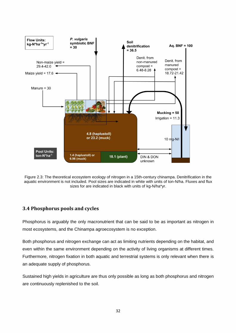
32

Figure 2.3: The theoretical ecosystem ecology of nitrogen in a 15th-century chinampa. Denitrification in the aquatic environment is not included. Pool sizes are indicated in white with units of ton-N/ha. Fluxes and flux

sizes for are indicated in black with units of kg-N/ha*yr.

3.4 Phosphorus pools and cycles

Phosphorus is arguably the only macronutrient that can be said to be as important as nitrogen in

most ecosystems, and the Chinampa agroecosystem is no exception.

Both phosphorus and nitrogen exchange can act as limiting nutrients depending on the habitat, and

even within the same environment depending on the activity of living organisms at different times.

Furthermore, nitrogen fixation in both aquatic and terrestrial systems is only relevant when there is

an adequate supply of phosphorus.

Sustained high yields in agriculture are thus only possible as long as both phosphorus and nitrogen

are continuously replenished to the soil.

33

The phosphorus cycle is quite different from the carbon and nitrogen cycles in that it doesn’t truly

possess an atmospheric component (Ågren and Andersson, 2012). Particulate matter lifted by the

wind can indeed transport phosphorus through the air, and in some special cases phosphine gas

can result from biomass decomposition, but neither of these phenomena is universal enough to be

considered in a model such as ours without explicit evidence of them taking place. In fact, most

naturally occurring forms of phosphorus have very low to no mobility in an ecosystem, taking the

shape of phosphate bound to either organic molecules, metal oxides and hydroxides, or calcium

minerals. Organic phosphorus is only as mobile as the organic matter it forms a part of, and is as a

rule insoluble and is found as part of soil particulates or biomass at different degrees of

decomposition. Inorganic phosphorus, almost exclusively found in the shape of phosphate, binds

strongly to iron oxides and aluminium hydroxides, forming in both cases insoluble compounds that

are largely unavailable for uptake by plants. Calcium-phosphate minerals tend to be insoluble as

well, although some of them more so than others. Among these, apatites are the least soluble.

Finally, even unprecipitated phosphate ions can adsorb strongly to both clay and organic particles

in the soil, making them largely biologically unavailable.

As a result of phosphorus’ low mobility and propensity to form insoluble minerals, abiotic processes

in the phosphorus cycle are of unusual importance, as changes in pH and the redox character of the

soil, as well as the presence or absence of clay minerals and inorganic ions, can entirely dictate the

mobility of phosphorus compounds in an environment.

Phosphorus being much less prone to leaving the soil system than nitrogen or carbon, there should

be relatively good documentation for the phosphorus content of soils and sediments in the

premodern chinampas of central Mexico coming from archaeological studies. Unfortunately,

phosphorus is rarely of any interest to archaeologists and physical anthropologists and thus, there

is very limited data on the phosphorus cycle of the ancient chinampas. In reality, phosphorus is likely

to be the least well-documented nutrient in the Chinampa system.

The quality of parent material is perhaps the most important factor influencing the size of the

phosphorus pools in an ecosystem, which makes the geological history of the region relevant for the

ecology of phosphorus as well. The central Mexican basin is located in a region of very recent

volcanism, and importantly, it was closed off from drainage into the Pacific ocean due to major

volcanic activity about 600,000 years ago (Solano and Vanegas, 2005). More recently, the trans-

Mexican volcanic belt experienced major activity in the 2nd and 3rd centuries AD from the Xitle volcano

and continuous minor to moderate activity by the Popocatépetl volcano since the seventh century

34

BC (Macías, 2007; Siebe, 2000). This activity has deposited numerous layers of volcanic ash on the

bottom of the basin, possibly adding to the content of primary phosphorus in the subsoil.

Such volcanic activity would initially indicate that the mountainous surroundings of the ancient lake

system were relatively rich in primary phosphorus minerals. However, no economically important

phosphatic rock deposits have been reported in the region (Appleton and Notholt, 2002) and no

comprehensive studies on the phosphorus content of neither the volcanic nor the alluvial deposits in

the basin could be located. This leaves us with no choice but to attempt to infer some aspects of the

phosphorus cycle indirectly.

Phosphorus is known to exist in a fairly consistent proportion of 13:1 to nitrogen in soils, including

those of wetland environments (Vepraskas and Craft, 2015). This puts, taking the nitrogen pools

calculated in the previous section as a starting point, the phosphorus pool of our chinampa at just

under 0.5 ton-P/ha for a monolithic dryland topsoil construction, and 2.3 ton-P/ha for a monolithic

chinampa made of wetland muck. The material in a plant-based foundation would have a P

concentration of 2.3 g-P/kg (Auclair, 1979), resulting in a foundation pool of 41.4 kg-P per chinampa,

or 2.76 ton-P/ha. Thus, a chinampa built on a foundation of aquatic plants would have a total

phosphorus pool of 4.56 ton-P/ha.

Frederick (Frederick, 2005) found quantities of up to 19 ppm of exchangeable phosphorus in the

buried ridged field material of ancient Xaltocan chinampas. This concentration would make a plant

available phosphorus pool of just under 122 kg-Pavailable/ha. Considering that unavailable phosphorus

typically represents 80-90% of the total pool in soil, this puts the latter in a range of 610-1220 kg-

P/ha, on the lower side of the values predicted from nitrogen pools. Thus, given that the limited

archaeological evidence available seems to fit the phosphorus estimates based on theoretical

nitrogen calculations, we will move forward with said theoretical values as total phosphorus pool

sizes, and attempt to estimate the main fluxes in and out of the soil.

Assuming that the most superficial sediment in the aquatic environment is made up primarily of dead

photosynthetic microbiota, macrophyte litter at different degrees of decomposition, and decomposing

microbiota, we can expect that the proportion of nitrogen to phosphorus in the sediment closely

follow Redfield’s ratio. Thus, having estimated a mucking flow of 50 kg of nitrogen per hectare per

year, and expecting an N:P ratio of 16, we can estimate the flow of phosphorus from mucking to be

3.1 kg-P/ha.

Irrigation during the drier months of the year could likewise move phosphorus from the aquatic

environment into the soil. Unfortunately, we find ourselves again lacking in direct data about the

35

phosphorus concentration in the canals of the ancient chinampas. Comparing using values from the

extant chinampa canals is unfortunately not an option in this case given that the original water

sources, along with the lake itself, no longer exist. Instead, we will remember that we consider the

canal environment to be eutrophic enough to allow intense autotrophic activity, particularly of

nitrogen-fixing cyanobacteria. Thus, we can estimate that the phosphorus concentration in the water

was at the very least as high as Redfield’s ratio would dictate for a good portion of the year. Thus,

the nitrogen concentration in water of 10 mg-N/L used before would imply a phosphorus

concentration of 0.62 mg-P/L, and a flux of phosphorus of 0.7 kg-P/ha*yr. It is perhaps worth noting

that Carney et al. (1993) measured similar concentrations of 0.21 to 0.43 mg-P/L in the inflow water

to the canal system of a raised field setting comparable to the premodern chinampas on the shores

of the high-altitude lake Titicaca (also an endorheic basin of volcanic origin).

Another input to the soil would come from human manure added either to composting plant litter or

directly to the soil. Since phosphorus has no significant gaseous form, we will not make a distinction

between manure added to compost or directly to the soil, although doing the former might play an

important role in the mineralization of nitrogen during composting of plant litter. Based on Knapp &

Denevan’s (1986) study of ancient and extant Ecuadorian raised-field agriculture, we could expect

an input of 7 kg-P/ha*yr from human and small animal manure, while a review of faecal composition

studies on modern humans would place this flux higher at 7 to 40 kg-P/ha*yr, depending on diet

(Rose et al., 2015).

Finally, harvest represents the major quantifiable outflow of phosphorus from the Chinampa soil.

With a maize grain yield of 3,000 kg/ha*yr, a water content of 71.4% and a phosphorus dry matter

content of 0.34%, 7.28 kg-P/ha*yr would have left the system in the form of maize grain. Using the

biomass export from non-maize harvest calculated before, 0.7-1.0 ton/ha*yr, and a mean

phosphorus content of 4 g-P/kg (4 g-P/kg for squash (Mohammad, 2004) and 3.9-4.0 g-P/kg for

beans (Araújo and Teixeira, 2003) the remainder of harvest represents an outflow of 2.8 - 4.0 kg-

P/ha*yr. Removals of this magnitude, when compared to the few inputs calculated before, point at a

rather tight phosphorus budget in the soil of our model chinampa (Equation 3.4 and Table 3.3).

Naturally, there are a number of fluxes not quantified here due to lack of information. Likely the most

important among these is the outflow of phosphorus from the soil to the aquatic environment in the

form of dissolved phosphate and particulate organic and mineral phosphorus-containing

compounds. Although we lack a reliable way to even estimate this flux, we can nevertheless outline

the main aspects in the premodern chinampa environment that would have governed it.

36

Three processes are of great importance in the mobility of phosphorus in primary and secondary

materials: solubilization of calcium-phosphorus minerals, dissociation of iron and aluminium

phosphate precipitates, and mineralization of phosphorus-containing organic molecules. These

three processes, however can respond to the same changes in the soil environment in different

ways. On the one hand, acidification can solubilize certain calcium-phosphate minerals, particularly

monophosphates and triphosphates, while at the same time facilitates the immobilization of

phosphate in the form of iron oxide and aluminium hydroxide minerals. Reciprocally, alkalinisation

can mobilize metal oxide and hydroxide-bound phosphate while decreasing the solubility of apatite

minerals. On the other hand, a change from oxidative to reductive conditions in the soil can mobilize

the phosphorus bound to ferric (charge 3+) iron by reducing it to ferrous (charge 2+) ions, but at the

same time greatly decelerate the decomposition of organic matter, thus helping keep phosphorus

fixed in insoluble organic molecules.

We can therefore expect that in the upper portion of the chinampa soil, leaching of carbonates

together under predominantly oxic conditions contributed to making iron and aluminium minerals the

main immobilizers of phosphorus, fixing what phosphorus was released from organic matter

decomposition to the extent to which these metals were abundant in the soil. This fixation would be

further amplified by the effect of humic acids from decomposition. Alkaline amendments, on the other

hand, would help mobilize some of the phosphorus for plant uptake.

Deeper in the soil, accumulation of leached calcium carbonates and predominantly anoxic conditions

would make calcium-phosphorus minerals the main immobilizer of any phosphorus that leached

down from the more active topsoil. Here, acidification from leached humic acids would be the main

phenomenon responsible for mobilizing phosphorus, allowing it to drain into the lake environment.

Parsons et al. (1986) determined that the pH changed throughout the first 2.3 m of the soil column

in a highly stratified buried chinampa in Mixquic, near Xochimilco. While the youngest buried

chinampa topsoil was acidic, with a pH well under 6, the soil became slightly alkaline in the layers

just below. Further down through what Parsons interprets as layers of cultivated surfaces of

increasing age, the soil pH rises and falls several times while remaining between 6.5 and 7. This

would seem to indicate that decomposition indeed acidified the topsoil, while in the soil below the

pH tended to be higher. Given the organic nature of the soil, however, it is possible that iron and

aluminium were not present in large quantities in the topsoil, thus allowing both for relatively high

rates of phosphorus plant uptake and leaching. The fact that the soil remained slightly acidic further

below the active surface of the could have helped further leaching of phosphorus into the lake

environment, helping to keep the phosphate concentration in the water high. It is possible that

37

leaching from raised beds acted as an unintentional mechanism that kept phosphorus contents in

the water high while slowly depleting the soil, allowing for high rates of microbial activity in the canals

and requiring large flows of both carbon and nitrogen onto the soil through mucking.

Knapp & Denevan (1986) in studying extant Ecuadorian raised fields does indeed note that the soils

and subsoils of the fields themselves were much poorer in phosphorus than the material that

accumulated in the ditches between them. This could support the idea of leaching into the

surrounding canals as another important loss of phosphorus from raised field agriculture in general.

Another interesting aspect of the phosphorus cycle in chinampas stems from the observations made

by Frederick (2005) in the strata predating the Xaltocan chinampas mentioned before. He measured

considerably lower phosphorus concentrations in the lacustrine deposits underlying both buried

chinampa beds and canal deposits than in the material deposited during the active life of the

chinampas. He measured 0.5 to 5.5 ppm of exchangeable phosphorus under the field ridges and

<0.5 to 9 ppm under the buried chinampa canals, while in the buried field and canal material these

concentrations ranged from 6 to 19 ppm and from 9 to 22.5 ppm, respectively. This would seem to

indicate that phosphorus in the lake environment was less abundant before the construction the

chinampas. However, judging by the fluxes identified so far there doesn’t seem to have been a

definite surplus in the phosphorus budget in the Chinampa ecosystem, and at any rate the main

input to the system seems to have been the water and sediment of the surrounding lake and canals.

How, then, did the establishment of chinampa agriculture propitiate an increase in deposited

phosphorus both soil and sediments while simultaneously allowing for intensive use of the soil?

Further inquiry into this matter would require considering the transport of dissolved and particulate

phosphorus from the surrounding basin into the lake environment and between different lake

compartments, as well as changes to the surrounding environments caused by human expansion

associated to the growth of Chinampa agriculture, a task that unfortunately is beyond the scope of

this thesis.

𝑀𝑢𝑐𝑘𝑖𝑛𝑔 + 𝑀𝑎𝑛𝑢𝑟𝑒 + 𝐼𝑟𝑟𝑖𝑔𝑎𝑡𝑖𝑜𝑛 − 𝐻𝑎𝑟𝑣𝑒𝑠𝑡𝑚𝑎𝑖𝑧𝑒 − 𝐻𝑎𝑟𝑣𝑒𝑠𝑡𝑛𝑜𝑛−𝑚𝑎𝑖𝑧𝑒 = ∆𝑃

Equation 3.4. Phosphorus balance in the premodern Chinampa system.

38

Table 3.3. Phosphorus budget of the theoretical premodern chinampa soil. All fluxes are in units of kg-P/ha*yr.

Flux IN OUT

Mucking 3.1

Irrigation 0.7

Manure 7

Maize harvest 7.8

Non-maize harvest 2.8 4.0

Budget

(In - Out)

Low values High values

0.2 -1.0

Figure 3.4 shows the local phosphorus cycle in the premodern chinampas of central Mexico to the

extent that it was possible to outline in this section. Unlike carbon and nitrogen, there is no clear

indication of surplus in the ecosystem, and it is possible there was a net loss of phosphorus from the

soil, making Chinampa agriculture dependent on constant imports from the lake environment or

elsewhere.

39

Figure 3.4: The theoretical phosphorus ecosystem ecology of the central Mexico chinampas as outlined from archaeological evidence, elemental analyses of modern versions of prehispanic crops and known

proportions between nitrogen and phosphorus concentrations in the environment. Pool sizes are indicated in white with units of ton-P/ha. Fluxes and flux sizes for are indicated in black with units of kg-P/ha*yr.

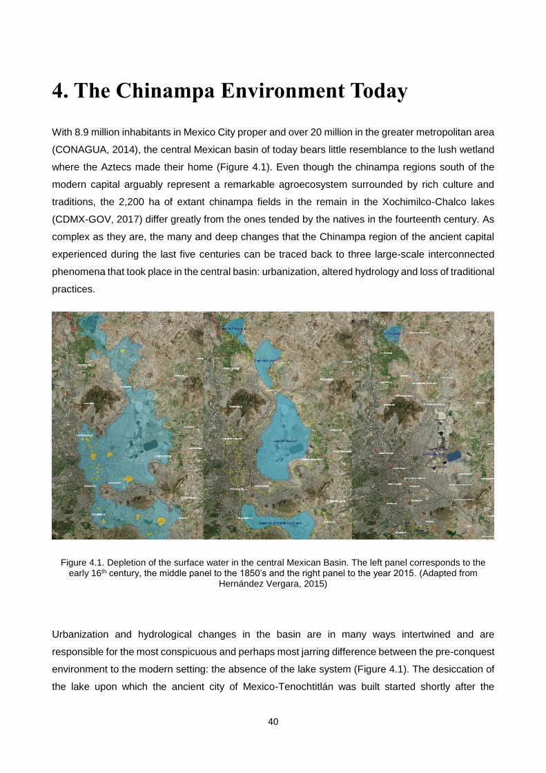
40

4. The Chinampa Environment Today

With 8.9 million inhabitants in Mexico City proper and over 20 million in the greater metropolitan area

(CONAGUA, 2014), the central Mexican basin of today bears little resemblance to the lush wetland

where the Aztecs made their home (Figure 4.1). Even though the chinampa regions south of the

modern capital arguably represent a remarkable agroecosystem surrounded by rich culture and

traditions, the 2,200 ha of extant chinampa fields in the remain in the Xochimilco-Chalco lakes

(CDMX-GOV, 2017) differ greatly from the ones tended by the natives in the fourteenth century. As

complex as they are, the many and deep changes that the Chinampa region of the ancient capital

experienced during the last five centuries can be traced back to three large-scale interconnected

phenomena that took place in the central basin: urbanization, altered hydrology and loss of traditional

practices.

Figure 4.1. Depletion of the surface water in the central Mexican Basin. The left panel corresponds to the early 16th century, the middle panel to the 1850’s and the right panel to the year 2015. (Adapted from

Hernández Vergara, 2015)

Urbanization and hydrological changes in the basin are in many ways intertwined and are

responsible for the most conspicuous and perhaps most jarring difference between the pre-conquest

environment to the modern setting: the absence of the lake system (Figure 4.1). The desiccation of

the lake upon which the ancient city of Mexico-Tenochtitlán was built started shortly after the

41

Conquest with the damming and diversion of all the major rivers that once nourished the Central

Basin with the purpose of making space for European-style agriculture and human settlements (Luna

Goyla, 2014). This early expansion of dryland against the original wetland was accompanied by two

very important technological departures from the traditional Chinampa system: the plough and the

large-scale cultivation of grain, often wheat and often in monoculture.

The practices of ploughing the soil and monoculture farming, together with European crops such as

wheat, have the very important effect of allowing for much more intensive use of the soil, accelerating

the decomposition of organic material in the topsoil and both boosting agricultural production and

rapidly depleting the soil from nutrients and organic material through the increased extraction of

nutrients by crops and leaching of excess nitrogen and phosphorus deeper into the soil and into the

water environment. Although the reason is still unknown, there seems to have been a post-Conquest

shift in the size of chinampas to much larger contiguous fields (Frederick, 2007). This change in

geometry, however, would have made ploughing easier on the raised beds, as larger even surfaces

are easier to till. Regardless of how it was introduced, the plough and the monoculture became fairly

universal technologies in the post-Conquest chinampas, to the extent that Santamaría (1912)

included the as fundamental aspects of the Chinampa tradition.

In later centuries after the Conquest, immense drainage works were made to carry rainwater away

from the Central Basin and out towards the north, in an effort to protect the growing city of Mexico,

now built mostly on the dry lake bottom, from constant floods (Bojorquez-Tapia et al., 2000; Luna

Goyla, 2014). The final depletion of the lake occurred during the second half of the twentieth century

as the now multimillion-people City of Mexico struggled to supply water to its rapidly growing

population, and began to deplete its groundwater resources (Krasilnikov et al., 2011; Moncada Maya,

1982). Overexploitation of the basin’s aquifers resulted in the in the drying of the springs and rivers

that nourished what was left of the Xochimilco-Chalco lakes as early as the year 1953 (Moncada

Maya, 1982), critically lowering the water level in its canals and lagoons.

This aggressive urbanization and hydrological depletion have led to further ecological alterations as

the progressive drying of the remaining Xochimilco lake was countered by increasing refilling with

sewage treatment outflow. This remedy began with a single local treatment plant built in 1959 with

the capacity of diverting 0.4 m3/s into the lake (Moncada Maya, 1982), and was gradually expanded

to eight wastewater treatment plants in the Xochimilco and Iztapalapa boroughs with a total refilling

capacity of 2.5 m3/s (CDMX-GOV, 2017).

Government-affiliated sources (CDMX-GOV, 2017) claim that the wastewater outflow that has come

to substitute the natural surface and groundwater resources in the Chinampa system in Xochimilco

42

is safe for agricultural use and low in both nutrients and pollutants. This claim is, however, disputed

by many independent sources that point out that the wastewater treatment facilities are not properly

designed for the removal of nutrient salts, organic pollutants, or heavy metals (Martínez Cruz et al.,

2006), resulting in the lake becoming not only eutrophic and potentially toxic, but also highly saline,

with sodium concentrations as high as 0.5 g/L. Furthermore, the use of open-air canals for the

transport of treated wastewater to the lake combined with the prevalence of irregular settlements in

the area result in around 17,000 homes directly discharging raw sewage to the lake, worsening the

nutrient and pollutant loads it receives and adding infectious faecal bacteria to the mix (Moreno,

2011; Perez-Montes et al., 2014; Zambrano González et al., 2012). Finally, a report from 2014 made

by the National Autonomous University of Mexico (P.U.M.A., 2013), stated that the actual volume of

treatment outflow water being fed to the lakes was less than a fifth of the planned diversion capacities

of the treatments plants, and was likely not enough to compensate for the lake’s losses from

percolation or agricultural use, adding insufficiency to the list of shortcomings in remedying the

depletion of the lake with sewage treatment outflow.

A recent study (Contreras Ruiz Esparza, 2012) carried out around the majority of the extant

chinampa canals of Xochimilco in both the rainy and dry seasons found median levels of,

respectively, 2.65 and 0.71 mg/L for ammonium, 2.59 and 4.03 mg/L for nitrate, and 10.23 and 6.31

mg/L for phosphate, with local seasonal levels as high as 13.4 mg/L for ammonium, 16.51 for nitrate

and 17.97 mg/L for phosphate. Oxygen levels below 30% saturation were found in 9 out of 27 sites

during the dry season, and in 7 out of 26 sites during the rainy season, with means of 46.02% and

43.78% respectively. All of these point at a highly eutrophic lake prone to experiencing oxygen

depletion. Besides the alarming environmental degradation stemming from anoxia and water

pollution in general, high concentrations of nutrients in the canal water coupled with an increased

need for irrigation caused by low lake stages year-round mean that the addition of nitrogen and

phosphorus through irrigation now takes a predominant role in the nutrient budgets of the extant

chinampa soils.

The vulnerability to water stress and drought caused by the receding water levels in the remaining

Chinampa canals, together with the salinity of the water and the risk of infectious disease from faecal

bacteria have all combined to greatly disincentivize Chinampa agriculture in recent decades,

resulting in many farmers abandoning their fields and looking for a livelihood in the surrounding

urban sprawl of Mexico City (Alcántara Onofre, 2005). Today, only 3.586 of the 20.922 surviving

chinampas in the Xochimilco-Chalco region are currently cultivated, and the main area of Xochimilco

is by far the most neglected, with only 864 active chinampas out of a total of 15,000 (CDMX-GOV,

2017).

43

Furthermore, abandonment of Chinampa agriculture has allowed for extant chinampas to be built

upon at an alarming rate; between 1989 and 2006, the Chinampa region in Xochimilco lost ground

to the city at a mean rate of 31 hectares per year (González-Esquivel, 2013).

This reduction, besides diminishing the total area of surviving Chinampa agriculture, also provokes

environmental changes on the remaining fields, likely further reducing the ameliorating effect thought

to have been an important element of the landscape (Crossley, 1999). Together with the

deforestation of practically the entire basin, the urbanization of the former Chinampa region has likely

made the extant chinampas more susceptible to the effects of droughts, heavy rainfall and winter

frost.

Abandonment has, however, been partially countered by the expansion of newer agricultural

technologies and a switch from sustenance horticulture to floriculture and ornamentals, particularly

in the younger generations. This means that in over half of the still-active extant chinampas the

ecology of the soil has been further changed by an abandonment of traditional techniques in favour

of greenhouses, mineral fertilizers and pesticides, the latter two often applied without proper

guidance (CDMX-GOV, 2017; González-Esquivel, 2013).

All these changes point at a much less efficient ecosystem ecology in the Chinampa system, where

recycling of local resources has lost much ground to the import of fast-acting animal manure and

commercial fertilizers. Thus, instead of a net habitat sink of nitrogen, and carbon, the chinampas of

today are likely net sources as ploughing and drying of the topsoil increases oxidation of organic

materials, and anoxic conditions in the highly eutrophic lake promote anaerobic losses of nitrogen to

the atmosphere.

Thus, the modern Chinampa agroecosystem finds itself in a vicious circle that is very hard to break.

The falling water levels in the canals due to the exhausted hydrology mean increased hydric stress

for crops and increased susceptibility to frost, as well as a deepening of the oxidative region in the

soil that together with the loss of traditional practices accelerate the loss of nutrients from the soil.

This, in turn promotes further abandonment of the Chinampa tradition in favour of expensive

agrochemicals or abandonment of the fields altogether. At the same time, urban encroachment and

aggressive abstraction of groundwater continue to degrade the lake environment due, in part, to the

diminishing cultural and economic importance of Chinampa agriculture in central Mexico.

44

In light of the many and complex threats to the lake remaining Xochimilco lake environment, it comes

as no surprise that the Mexican scientific community has forecast a complete disappearance of

Chinampa agricultural tradition during the 2020’s should the rate of environmental degradation

continue at its current pace (González-Esquivel, 2013).

45

5. Methodology

5.1 Soil Core and Water Sampling

5.1.1 Site selection

Contact was established with the Mexican conservation and education-oriented civil organization

Humedalia A.C., which agreed to support this study with both access to their field station for sampling

and by acting as caretakers of experiments performed on-site.

The Humedalia field station, an experimental chinampa itself, is located in the heart of the

conservation area of the Xochimilco lake, in Mexico City (Figure 5.1), at an altitude of 2,243 masl,

experiencing over 600-1000 mm of annual precipitation and a mean annual temperature of 16°C,

with a rainy season running from late spring to early fall. The site, located about 1 km from the urban

sprawl of the old Xochimilco town, was reached by water from Cuemanco, the lake access nearest

to the Periférico city ring road, 2 km away in a straight line.

The raised bed itself is about 30 m broad and about 100 m long, with an incomplete secondary canal

running along its middle from front to back, and rises over 1 m from the water level in its surrounding

canals. Its date or method of construction is completely unknown, as the Humedalia A.C.

organization has only managed it since 2014. One half of its front portion is kept with short grass

lawn and houses a roofed and tiled break area. Most of the remainder is currently in use as a testing

ground for Biointensive Agriculture integrated with elements of traditional chinampa agriculture, and

thus envelops a variety of soil uses while still consisting of a single morphological unit.

46

Figure 5.1: Field work area location in Mexico City. Base layers: Google Satellite & Open Street Maps

This way, it was possible to extract samples from soils exposed to different management regimes in

the medium and short term but that shared the same geological and pedological origin. Five sites

were selected for soil sampling within the Humedalia A.C. chinampa location (Figure 5.2), all of which

in this report are denoted with the prefix HS:

• HS1. A bed near the edge of the chinampa, easily accessible from the surrounding canal,

used as an almárcigo or muck-based plant nursery.

• HS2. A bed further into the chinampa used for horticulture. The soil in this site is had recently

been ploughed, amended with compost and mulched with dry grass following the

Biointensive practice (Roberts, 2018), awaiting transplantation of plantules from one of the

nursery beds at the time of sampling.

• HS3. Grass lawn near a roof structure. Mowed regularly and watered with canal water in the

same manner as the crops.

47

• HS4. A cleared patch of soil. Originally intended as an active horticultural bed, it is currently

used as access to a secondary canal for irrigation.

• HS5. Wild. At the time of sampling completely overgrown with wild plants, primarily the

seasonal wild cucurbit Sicyos deppei.

Figure 5.2: Placing of HS and SW sampling sites.

48

It was discovered during preliminary field observations, however, that the water table in the

Humedalia (HS) location and all surrounding chinampas had permanently receded to more than 1 m

below the surface due to falling water levels in the lake, a characteristic that set the HS sites apart

from the theoretical Chinampa model. This prompted the search for a chinampa with a lower profile,

and therefore a shallower water table. Such a site was located about 1,400 m east from the HS sites.

The SW1 site was located in the middle of the small SW chinampa (Figure 5.2) and corresponded

to an agricultural soil more closely resembling the traditional chinampa model, with groundwater

roughly 40 cm below the surface at the end of the rainy season (September-October), where instead

of mucking, the soil was amended with crushed water plants (primarily water hyacinth) as green

manure using a 15 cm plough.

Images of all sites are presented in Annex A.

5.1.2 Soil core extraction

One 1 m-long soil core was extracted using a metal auger at each site, for a total of six cores. Due

to the colour and texture homogeneity of the soil throughout the entire first meter, the soil cores were

not divided according to horizons, but in arbitrary intervals.

To provide adequate depth resolution, all cores were divided in 10 cm, intervals, except when there

was a clear change in texture, at which point an extra boundary was placed.

This caused the core HS1 to consist of eleven fractions, given that the bottom 5 cm in the core were

clearly wetter and more clay-like than the rest of the core’s material.

In the case of HS2, the loose, recently ploughed and amended topsoil crumbled out of the auger

upon extraction, for which the first 15 cm had to be extracted again right next to the initial excavation

site.

All core fractions were placed in a paper bag labelled with site, depth and any relevant observations

immediately after extraction and frozen at -20°C upon return from the field.

Two weeks later, the paper bags containing the core samples were placed open in a gas oven at a

temperature between 80 and 100 degrees for six hours, or until dry to the touch.

The dry samples were transported from Mexico to Denmark in a closed plastic bag as regular

luggage in a commercial flight, with a total travel time of 15 hours. All core samples were frozen

again upon arrival in Denmark.

49

5.1.3 Bulk density sample extraction

Besides the soil cores, mainly destined for element and nutrient tests, bulk density samples were

extracted using a 100 ml bulk density ring from the sites HS1 (at 0, 10, 25, 40 and 50 cm of depth),

HS2 (topsoil only), HS4 (0, 20, 40, 60 and 90 cm of depth), and SW1 (0, 25 and 40 cm of depth).

The soil was excavated by hand using a trowel until the desired depth was reached and the ring was

pushed carefully into the soil using the trowel’s handle. After extraction, the ring’s contents were

carefully poured into separate paper bags labelled with site and depth and stapled closed.

Bulk density samples, referred from here on as “Ring” samples, were kept frozen, dried and

transported in the same manner as the core samples.

5.1.4 Canal water and groundwater sampling

Canal water samples were collected by hand at 0 -10 cm depth from five random sites around the

SW location to serve as a comparison to the site’s ground water samples.

Ground water samples were taken at the SW location by digging with a small shovel at the middle

of the chinampa (5 meters on the narrow side and 10 meters on the broad side from the nearest

canal) until encountering saturated soil, letting water accumulate freely and collecting it by hand by

quintuplicate in plastic phials. During the September-October field work, water was observed as

close to the surface as 40 cm. In the December visit, however, when the groundwater samples were

taken, the water table was located deeper, closer to 70 cm below the surface.

5.2 Muck decomposition experiment

To investigate the short-term changes in the lake muck added to the topsoil in traditional Chinampa

practices, an experiment was carried out where muck was exposed to atmosphere, temperature and

soil microfauna in a manner analog to either the environment of an almárcigo plant nursery or to a

newly mucked traditional bed. Samples were taken periodically and promptly frozen in an effort to

preserve a time series of “snapshots” in the decomposition process of the rich lake sediment. Muck

extraction and experiment setup were carried out personally, after which the maintenance of the

experiment was taken over by Diego Hernández from the local Humedalia A.C. work group.

An initial attempt at this experiment was carried out in the fall of 2017 between October 4th and

October 25th, spanning three weeks of sampling. Although initially planned for ten weeks of duration

and sampling, this experiment run was stopped early due to a scheduling conflict.

50

The experiment was repeated during the following winter between December 26th and February

28th, spanning a full ten weeks of exposure.

The samples in both occasions were shipped from Mexico City to Copenhagen through a commercial

package delivery service inside a Styrofoam cooler complemented with gel cooling elements. The

samples were verified to still be in a frozen state upon arrival and monitoring with a temperature

logger showed that the temperature at the centre of the box did not exceed 0 degrees Celsius during

the two-day travel.

5.2.1 Muck extraction

Lake sediment, or muck, was extracted in both experimental runs by the Humedalia A.C. personnel

as part of their seeding procedure. The procedure consists of rowing a shallow canoe in the access

canals surrounding the Chinampa and collecting sediment where it appeared less sandy using a

long-shafted shovel, collecting it on the bottom of the canoe (Figure 5.3).

Figure 5.3: Diego Hernández from Humedalia A.C. transporting lake sediment back to the experimental site for seeding and muck decomposition experiment. October 2017.

5.2.2 Experiment setup

The muck was cleaned by hand from rocks, plastic litter and plant debris upon return to the

Chinampa. During the process of transferring the muck from the canoe to the new nursery bed, a

small portion (about three kilograms) was gradually set apart for the experiment by taking small

portions at random points of the transfer.

51

This muck was poured into three shallow polypropylene tubs (roughly 20 x 35 x 15 cm) filled with

about 2 cm of soil from an adjacent resting almárcigo (that is, where all viable plugs had previously

been transplanted to a growing bed) as inoculum for soil microfauna.

Draining holes had been drilled into the bottom of the three tubs using a 2 mm bit at regular 5 cm

intervals. The lids of the tubs had been cut, replacing all but the clamping edges with plastic mesh

to allow free gas exchange with the outside while keeping new macrofauna and opportunistic seeds

out.

The tubs containing the muck were placed in the shade under a straw roof structure built on the

same Chinampa roughly 10 m away from the nursery beds (Figure 5.4).

Figure 5.4. Muck decomposition experiment setup. Fresh sediment filled into polypropylene tubs with drain holes (top) and closed tubs with mesh lids in a shaded and roofed location (bottom).

52

5.2.3 Sediment sample extraction and storage in Mexico

Upon filling the tubs with sediment, one “zero” sample was taken from each tub by scooping small

amounts of fresh muck into sealable polyethylene bags (Fig 5.4, top). When the muck finished

draining its excess water (roughly 48 hours after filling), square plugs analogue to those used in

nursery beds were cut into all three tubs of muck. After this point, the Humedalia A.C. work group

took over maintenance and sampling of the experiment.

The caretakers were instructed to maintain the experiment moist as they would in a plant nursery

(through visual inspection), watering with bottled drinking water when necessary, but taking care not

to saturate the samples. Any plants or terrestrial macrofauna were to be removed from the

immediately if spotted.

Once a week for a period of ten weeks, starting seven days after the “zero” sampling, one random

plug of muck was removed from each tub, and placed in a separate labelled sealable polyethylene

bag. While in the field, the samples were to be kept inside a polystyrene cooling box filled with gel

cooling elements. By the end of the work day at the Chinampa, the samples would be taken home

by a member of Humedalia A.C. and placed in a household freezer at ca. -20°C until the experiment

was completed.

Other than when performing cleaning or sampling operations, the lids were to be kept securely on

the tubs at all times.

5.3 Soil Properties Analysis

5.3.1 Bulk Density

The Ring samples were transferred to small aluminium trays, taking care not to lose material in the

process, and dried at 105°C for 24 hrs without grinding. All ring samples were weighed accurately

afterwards to determine bulk density.

5.3.2 Organic Matter Content

The Ring samples were taken from storage and re-dried overnight at 105°C. Afterwards, subsamples

of about 5 g were placed in pre-weighed clean porcelain crucibles and weighed precisely. These

subsamples were placed in a muffle oven at 550°C for 1 hr and afterwards let cool down in a

desiccator. Once at room temperature, the subsamples were weighed again.

53

5.3.3 CaCO3 Qualitative Test

Small random portions (ca. 0.5 g) of the ground and mixed ring samples were placed on a porcelain

dish and 2% HCl was dripped slowly on them, visually inspecting for bubble formation.

5.4 Nutrient Analyses

5.4.1 Total Carbon and Total Nitrogen by Organic Elemental Analysis

All Core samples were dried at 105°C for 24 hrs and let cool down inside a desiccator bell. About 15

mg of each depth fraction were weighed precisely and packed into tinfoil capsules in triplicates,

which were kept in a desiccator bell until analysis in an organic elemental analyser in CHN mode

(without sulphur determination) with a copper column and oven temperature of 1200°C.

5.4.2 Total phosphorus in Core samples by ICP-MS

Microwave digestion and extraction commonly used in ICP-MS was substituted in these analyses by

the method described below, adapted from colorimetric procedures (Geografisk Institut Laboratoriet,

Metode 5A, 1999) to reduce the number of steps in the extraction and increase the number of

samples that could be extracted simultaneously. To ensure the reliability of the adapted method, the

total P content of the HS1 bulk density ring topsoil sample was analyzed in five replicates both after

microwave digestion (31 min at 600W with 6 ml HNO3- 65% w/w), and the adapted method. This

preliminary comparison showed neither a significant difference (p=XX, one-way ANOVA) between

methods nor an important variability between repetitions (Fig. 5.5).

54

Figure 5.5. Comparison of microwave extraction versus combustion at 550°C in a muffle oven followed by

extraction at 70°C in a sandbath. Both procedures were performed using HNO3- 65% and analyzed in the

same ICP-MS run.

All core samples were dried, one or two full cores at a time, at 105°C overnight and one ca. 0.5 g

subsample was taken from each depth fraction of each core, weighed precisely and placed in a clean

porcelain crucible. These subsamples were burned at 550°C in a muffle oven for 1 hr and let cool

down to room temperature. Then, the subsamples were placed in a sand bath at 70°C and 6 ml

HNO3- 65% w/w were added to each. The sand bath was allowed to reach 70°C after the filling

procedure and the samples let react for 10 minutes, after which they were taken out and let cool

down to room temperature for 1 hr.

The resulting extract was filtered through a glass fibre circle filter into a 200 mL volumetric flask and

filled with triple-deionized water.

This procedure was performed in triplicate for all six cores (61 core samples, 183 Core subsamples

analysed in total).

Method blanks were included in three separate occasions to control systematic error due to the

extraction procedure. These samples were prepared on empty clean crucibles following otherwise

the exact same procedure as with soil core samples.

55

All soil core extracts were analyzed in an ICP-MS in helium mode with a helium flow of 0.5 ml/s after

a standard row comprised of 100, 200, 500, and 1,000 ug-P/L. A system standard was repeated

every 10th analysis to control for drift, which, when present, was corrected using a linear function.

5.4.3 Canal Water Sample Preparation

The five groundwater replicate samples and five canal water samples were thawed at 5 degrees for

24 hrs, after which they were filtered using paper circle filters on glass funnels. The filtered water

samples were the frozen again and kept in this manner until tested.

5.4.4 Phosphorus Analysis of Groundwater and Canal Water by ICP-MS

The filtered groundwater and canal water samples were thawed inside a refrigerator and kept closed

at all times. 5 ml of each sample were transferred into 100 ml glass volumetric flasks. The flasks

were then added 3 ml HNO3- 65% and filled with triple-deionized water. Approximately 5 ml of these

dilutions were transferred into plastic vials for ICP-MS analysis in helium mode with a helium flow

of 0.5 ml/s after a standard row comprised of 100, 200, 500, and 1,000 ug-P/L.

5.4.5 Muck decomposition experiment (EXP) sample water content determination and

preparation

Water content determination was only performed on the October 2017 experiment (EXP) samples.

The December-February EXP samples were dried and prepared in the same manner, but water

content was not measured.

A subsample about 2 cm thick was cut along the long side of each frozen EXP plug sample (in order

to include both top and bottom of each sample, assuming it to be otherwise symmetrical) and

weighed. Then, each subsample was dried at 105°C for 24 hrs, let cool down in a desiccator and

weighed again for water content determination. The dry subsamples were then ground manually in

a porcelain mortar and kept covered on a workbench until further preparation and analysis.

5.4.6 Total Carbon and Nitrogen by Organic Elemental Analysis

All dry EXP subsamples were re-dried overnight at 105°C and let cool down inside a desiccator bell.

About 15 mg of each subsample were weighed precisely and packed into tinfoil capsules. The

October subsamples were prepared for analysis in triplicates, while the December-February samples

were prepared in singlets, as the EXP samples themselves were considered to be triplicates of the

same treatment. The weighed prepared subsamples were kept in a desiccator bell until analysis in

56

an organic elemental analyser in CHN mode (without sulphur determination) with a copper column

and oven temperature of 1200°C.

5.4.7 Total and Inorganic Phosphorus Acid Extraction

Only subsamples from the October EXP samples were prepared and analysed for total and inorganic

phosphorus content. Two portions of approximately 0.5 g were taken from each dry EXP subsample

and placed into a porcelain crucible and weighed precisely. One of the two portions was then burnt

in a muffle oven at 550°C for 1 hr and let cool down to room temperature.

The crucibles with all burnt and unburnt portion were placed in a sand bath at 70°C and added 5 mL

H2SO4 6M, where they were let react for 10 minutes after reaching 70°C. Subsequently, the

crucibles were let cool down at room temperature for 1 hr. with a second addition of 5 ml H2SO4

6M.

The resulting extracts were diluted in approximately 100 ml triple-deionized water in disposable

plastic cups and subsequently filtered with several washings using paper circle filters into 200 ml

volumetric flasks.

5.4.8 Olsen (Labile) Phosphorus Extraction

A portion of approximately 0.5 g was taken from each dry EXP subsample, weighed precisely and

placed in a disposable plastic cup with a lid. Each portion was added 40 ml CaCO3 0.5M and shaken

for 1 hr. The extract was filtered and rinsed into 200 ml volumetric flasks using paper circle filters.

5.4.9 Phosphorus Analysis in EXP subsamples by Colorimetry

Total, inorganic and Olsen phosphorus in EXP subsamples were determined via the

spectrophotometric quantification of dissolved orthophosphate in reaction with ammonium

heptamolybdate decahydrate, antimony iron(III) oxide and ascorbic acid.

An inactive color reagent stock was prepared by dissolving 12.8 g of Ammonium heptamolybdate

decahydrate and 0.31 g of potassium antimony(III) oxide tartrate in 3.8% H2SO4 inside a 2,000 ml

volumetric flask.

A fresh 500 ml batch of active color reagent was prepared on each day of analysis by dissolving

3.00 g ascorbic acid in inactive color reagent inside a 500 ml volumetric flask.

57

30 ml of sample extract were mixed with 10 ml active reagent in a 100 ml volumetric flask, filled with

triple-deionized water, shaken thoroughly and let develop color for 15 minutes, after which 2 ml were

poured into a plastic cuvette and placed in a spectrophotometer set for absorbance at 890 nm.

Standards (0.05 mgP/L, 0.10 mgP/L, 0.30 mgP/L, 0.50 mgP/L and 1.0 mgP/L) were prepared on each

day of analysis using different volumes of 1:1000 and 1:100 dilutions of an analytical standard

solution 1000 mgP/L mixed into 100 ml volumetric flasks filled halfway with triple-deionized water,

added 3 ml H2SO4 6M and 10 ml active color reagent, filled to the mark, and let develop for 15

minutes before spectrophotometric analysis at 890 nm.

5.4.10 KCl extraction from wet EXP samples and top Core samples

Only subsamples from the October EXP samples and the 0 cm Core samples of all sites were

prepared in this manner.

A subsample approximately 1 cm in thickness was cut along the long side of each frozen EXP

sample, placed in a disposable plastic cup with a lit and weighed precisely. 40 ml KCl 1M were added

and the mixture shaken for 1 hr. The extract was filtered into airtight plastic phials using 0.2 um

syringe cartridge filters and immediately frozen at -18°C to await analysis.

5.4.11 Ammonium Analysis of Top Core, EXP and Water Samples by Colorimetry

KCl extracts of the top (0 cm) Core samples and October EXP subsamples, as well as paper filtrates

of SW1 groundwater and canal water samples were tested in this manner.

Fresh batches of sodium salicylate-sodium nitroprusside (440 g + 0.22 g) reagent and alkaline

sodium tricitrate (120 g in ~0.5M NaOH sol.) reagent were made separately and kept refrigerated for

no longer than three months.

2.5 ml of 1:100 dilutions of all October EXP subsample and top Core sample KCl extracts, as well

as 1:10 dilutions of all groundwater and canal water samples were placed in new polypropylene

sample tubes. To these tubes were added 500 uL of a 1:27 mixture of 10% sodium hypochlorite and

the sodium tricitrate batch reagent, and 300 uL of sodium salicylate-sodium nitroprusside batch

reagent.

An external standard curve with NH4+ concentrations of 0, 5, 10, 20, 30, 40, 50 and 100 uM was

prepared from NH4Cl dried at 60°C for 1 hr, using KCl 0.01M as solvent to match the composition of

EXP and Core samples.

58

Immediately after mixing and vortex shaking, all sample and standard tubes were let react in the

dark for 2.5 hrs, then transferred immediately to plastic cuvettes for spectrophotometric quantification

at 640 nm.

5.4.12 Nitrate Analysis of Top Core, EXP and Water Samples by Flow Injection Analysis

KCl extracts of the top (0 cm) Core samples and October EXP subsamples, as well as paper filtrates

of SW1 groundwater and canal water samples were tested in this manner.

All samples were analyzed by the staff of the Institute for Nature and Environment at Roskilde

University, using the method of reduction to nitrite with a copperized cadmium column, followed by

diazotization by sulfanilamide under acidic conditions and reaction with N-(1-

naphthyl)ethylenediamine dihydrochloride to form a pink dye. Absorption was measured

spectrophotometrically at 520 nm in a Flow-Injection Analysis setup.

59

6. Results and Analysis

Tables summarizing all results are presented in Annex B

6.1 Soil Properties

Figure 6.1. Collage of Core samples. From top to bottom, HS1, HS2, HS3, HS4, HS5 and SW1.

60

The soil at all sites in both locations is, as one might expect, very high in organic material. This gives

the soil an almost completely homogeneous texture and colour throughout the first meter from the

surface: black and pliable when moist, black and slick, slightly sticky when wet, and dark gray when

dry. On the bare soil of site HS4, white salt crusts were spotted on the dry surface. The visual

appearance of the extracted cores is shown in Fig. 6.1.

6.1.1 Bulk Density

Bulk density measurements in the HS location and the SW location show that the first meter of the

soil tends to be lighter at the top and heavier further down (Figure 6.2). The active sites HS1 and

HS2 (not shown in the figure) both had relatively low densities at the surface, respectively 0.3 ton/m3

and o.35 ton/m3. The bare topsoil at site HS4 is more compact, with a bulk density at the surface of

just under 0.55 ton/m3. However, the bulk density of HS4 decreases to under 0.4 ton/m3 at 20 cm

of depth, below the value of both HS1 and SW1 at similar depths.

At 25 cm of depth and below, both HS1 and HS4 become denser with depth, reaching 0.56 ton/m3

and 0.62 ton/m3, respectively, at 40 cm of depth. From that point, soil density seems to taper down

for both sites, falling more quickly for HS1 to just under 0.5 ton/m3 at 50 cm of depth than for HS4,

which reaches the same density first at 90 cm of depth.

The SW1 site behaves different than the soils of the HS location, in that its density changes very

little with depth down to a shallow water table just below 40 cm of depth. Its bulk density at the

surface is just over 0.4 ton/m3, rising to 0.5 ton/m3 at 25 cm of depth and falling slightly to 0.47

ton/m3 at 40 cm.

61

Figure 6.2. Bulk density measurements taken in the plant nursery and bare soil sites of location HS, and in the shallow water table site SW1. All bulk density samples were taken in September 2017, at the end of the

rain season in central Mexico.

6.1.2 Soil Organic Matter

The soil organic matter (SOM) in the samples sites is shown in Figure 6.3. In the almárcigo plant

nursery site, HS1, the constant addition of lake sediment is quite visible in the very high SOM content

at the surface. The routine removal of the sediment plugs containing sprouted plantules is also visible

in the shape of a steep decrease of SOM below the uppermost 10 cm.

In site SW1, the soil has a rather constant SOM content throughout the upper 40 cm, despite it being

periodically tilled to a depth of 15 cm.

Interestingly, the bare soil at the top of HS4 has nearly the same SOM content as the moist topsoil

of SW1, even though it is considerably drier. Furthermore, this site shows an unusual accumulation

of organic matter at around 20 cm of depth, reaching up to 25% SOM. This accumulation zone seems

to stop completely at 40 cm of depth, where the SOM content falls to 14%, nearly identical to HS1

in spite of the very different uses that these two sites are given.

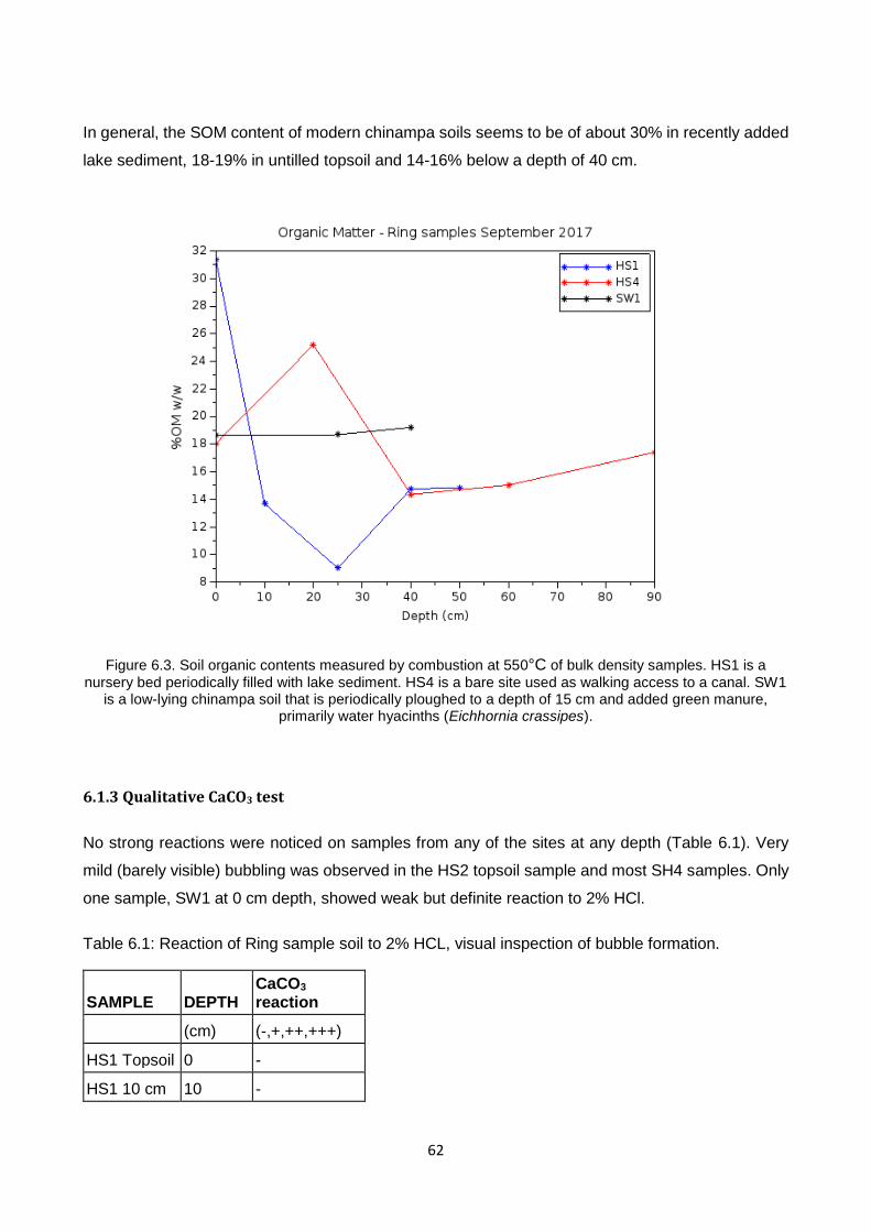
62

In general, the SOM content of modern chinampa soils seems to be of about 30% in recently added

lake sediment, 18-19% in untilled topsoil and 14-16% below a depth of 40 cm.

Figure 6.3. Soil organic contents measured by combustion at 550°C of bulk density samples. HS1 is a

nursery bed periodically filled with lake sediment. HS4 is a bare site used as walking access to a canal. SW1 is a low-lying chinampa soil that is periodically ploughed to a depth of 15 cm and added green manure,

primarily water hyacinths (Eichhornia crassipes).

6.1.3 Qualitative CaCO3 test

No strong reactions were noticed on samples from any of the sites at any depth (Table 6.1). Very

mild (barely visible) bubbling was observed in the HS2 topsoil sample and most SH4 samples. Only

one sample, SW1 at 0 cm depth, showed weak but definite reaction to 2% HCl.

Table 6.1: Reaction of Ring sample soil to 2% HCL, visual inspection of bubble formation.

SAMPLE DEPTH CaCO3 reaction

(cm) (-,+,++,+++)

HS1 Topsoil 0 -

HS1 10 cm 10 -

63

HS1 25 cm 25 +

HS1 40 cm 40 -

HS1 50 cm 50 -

HS2 Topsoil 0 +

HS4 Topsoil 0 +

HS4 20 cm 20 +

HS4 40 cm 40 +

HS4 62 cm 60 +

HS4 90 cm 90 -

SW1 Topsoil 0 ++

SW1 25 cm 25 +

SW1 40 cm 40 +

6.2 Nutrient Analysis on Core samples

All nutrient analyses on Core samples were performed on dry material stored at room temperature.

It is, however, highly unlikely that this affected any of the analyses with the exception of ammonium

content, as it is possible that the drying process removed important amounts of ammonia gas from

the soil. Thermal decomposition of nitrogen-containing organic compounds is not expected to be

important at 105°C. Phosphorus, having no important gas forms in soil, is not likely to be affected by

drying.

Total carbon and total nitrogen analyses proved to be highly reliable, with minimal variability between

repetitions of the same sample. Nitrate and ammonium analyses were not repeated enough times

to get a proper notion of the repeatability of the extraction method, but no problems were immediately

visible. The phosphorus analyses were by far the most problematic, showing high degrees of

variability between repetitions of the same sample. This variability is unlikely to reflect an

inhomogeneity in the soil samples, as these were thoroughly ground and mixed during preparation,

and they exhibit none of the same behaviour in total carbon and nitrogen analyses. Contamination

during the process is also very unlikely, since the several method blanks introduced in the

phosphorus analyses consistently showed concentrations below the detection limit of the mas

analyser.

Therefore, the high variability of phosphorus analyses by ICP-MS in Core samples can be attributed

to elemental interferences and deficient ionization during the plasma stage of the ICP-MS

64

measurements, or to stochastic human error during sample preparation and extraction. It is

noteworthy that ICP-MS is not usually the preferred technique for phosphorus quantification, since

phosphorus tends to have low response factors in this technique, and due to its low atomic weight

can also be occluded by many different elemental and molecular interferences. Further work is

needed to develop a proper procedure that takes advantage of the speed and sensitivity of ICP-MS

without suffering from its drawbacks.

6.2.1 Total Carbon and Total Nitrogen by Organic Elemental Analysis

When superimposed (Fig. 6.3 top and bottom), all six cores can be compared to estimate the

composition of the material below the surface, as well as the difference in organic elemental

composition caused by different processes in the soil.

A prominent feature in both sets of profiles is a high concentration of both carbon and nitrogen below

60 cm of depth, most visible for HS1, HS4, HS5 and SW1, that seems to indicate an accumulation

of organic matter. The carbon concentration in this region reaches values of over 14% for HS1 and

SW1, while it is lower in HS4 and HS5.

Looking closer to the surface of the soil profile, there are clear differences in carbon and nitrogen

concentrations between sites. While most profiles have carbon contents between 7% and 10% and

total nitrogen contents of 0.5% to 0.8% at the surface, HS1 has remarkably higher contents, over

17.5% and 1.2%, respectively.

In spite of being regularly amended with plant litter compost and animal manure, the topsoil of HS2

is the poorest among all sites, with about 7% total carbon and 0.5% total nitrogen contents. It is worth

noting, however, that even these values are relatively high compared to nearby conventional

agricultural soils. The profile of the lawn-grass site, HS3, has a relatively high concentration of both

carbon and nitrogen at the surface, over 9.5% and 0.75% respectively, yet is conspicuously poor in

SOM throughout most of the first meter, having lower concentrations of both elements than all the

other sites at all depths below 10 cm.

Finally, SW1 has very similar carbon and nitrogen concentrations to those of the two untended sites,

HS4 and HS5, at the surface. As depth increases, however, the concentrations of both elements in

SW1 increase steadily with depth surpassing those of all the other profiles, and peaking in the

accumulation zone described above. Interestingly, even though the carbon content of SW1 is lower

than that of HS1 in the bottom 30 cm of the profile, its nitrogen content is higher.

65

Figure 6.3. Total carbon and total nitrogen contents or soil core samples at 10 cm intervals. The error bars indicate the standard error of the measurement.

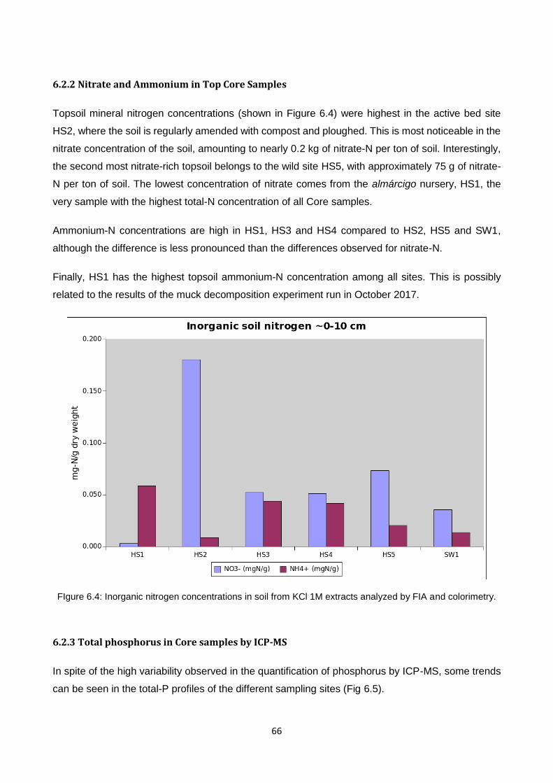
66

6.2.2 Nitrate and Ammonium in Top Core Samples

Topsoil mineral nitrogen concentrations (shown in Figure 6.4) were highest in the active bed site

HS2, where the soil is regularly amended with compost and ploughed. This is most noticeable in the

nitrate concentration of the soil, amounting to nearly 0.2 kg of nitrate-N per ton of soil. Interestingly,

the second most nitrate-rich topsoil belongs to the wild site HS5, with approximately 75 g of nitrate-

N per ton of soil. The lowest concentration of nitrate comes from the almárcigo nursery, HS1, the

very sample with the highest total-N concentration of all Core samples.

Ammonium-N concentrations are high in HS1, HS3 and HS4 compared to HS2, HS5 and SW1,

although the difference is less pronounced than the differences observed for nitrate-N.

Finally, HS1 has the highest topsoil ammonium-N concentration among all sites. This is possibly

related to the results of the muck decomposition experiment run in October 2017.

FIgure 6.4: Inorganic nitrogen concentrations in soil from KCl 1M extracts analyzed by FIA and colorimetry.

6.2.3 Total phosphorus in Core samples by ICP-MS

In spite of the high variability observed in the quantification of phosphorus by ICP-MS, some trends

can be seen in the total-P profiles of the different sampling sites (Fig 6.5).

67

The most striking difference is the phosphorus profile of the low-lying chinampa of site SW1. The

mean concentration of total phosphorus in this site is higher than in all the other sites at all depths,

particularly at the surface, where it has a mean concentration nearly twice as high as the topsoil of

all HS sites. This abundance of soil phosphorus, particularly considering that the SW1 site did not

have an exceptionally high SOC or total-N content compared to the other sites, could be caused by

high soil alkalinity, which would also explain the high variability in some of the measurements, as

acid extraction often performs poorly in basic matrices.

Another conspicuous feature of the phosphorus profiles is depletion zone localized at 10 cm depth

in the lawn site, HS3. This depletion zone likely coincides with the depth of maximum root density in

the lawn rhizosphere, and reflects the high P demand of keeping such a surface.

Otherwise, there is relatively little difference in the phosphorus content among all profiles other than

SW1.

Overall, the phosphorus contents of the HS sites range from 0.7 mg/g to just under 1.0 mg/g at the

surface, and gradually decrease with depth to minimum mean values between 0.3 and 0.6 mg/g at

depths between 60 and 85 cm, with little difference among sites. At the bottom of all cores, 90 and

95 cm of depth, phosphorus concentrations seem to rise again, although this increase is not as clear

as in total carbon and nitrogen profiles.

68

Figure 6.5. Mean total phosphorus concentrations in Core samples measured by ICP-MS. The bars represent the standard error in the measurements. HS1 samples were measured in quintuplicate due to their

high variability. HS2 were measured in quadruplicate. All other Core samples were measured in triplicate.

6.3 Nutrient analysis in Muck Decomposition Experiment (EXP) Samples

6.6.1 Total Carbon and Total Nitrogen in EXP Samples

As would be expected from any highly organic soil matrix after a change from anaerobic to aerobic

conditions, decomposition is visible in both the total carbon (Fig. 6.7) and total nitrogen (Fig. 6.8)

contents of the extracted subsamples.

There seems to be, however a strong difference in the rate of loss of both total carbon and nitrogen

from the sediment between the October and the December-February runs. In the former, nearly 2%

69

of the initial total carbon and over 0.1% of the initial total nitrogen are lost in the span of 21 days,

where in the latter run only about 1% of the initial total carbon and less than 0.05% of the initial total

nitrogen are lost during the total run of 64 days. The sediment used in the October experiment is

only slightly more nitrogen rich than the one set up in December, with a starting C:N ratio of 13.4

against 13.9, respectively, and this does not seem to substantially alter the general nutrient regime

of the decomposing muck.

Since temperature can be an important factor in organic matter decomposition rates, it is worth

accounting for climatic differences between the October and the December-February runs.

Climatological data does not suggest a very large temperature difference between October and the

months of January and February in Xochimilco (Fig. 6.9), the Humedalia A.C. group reported several

days of frost at the start of 2018 (personal communication).

Finally, the sudden apparent loss of carbon and nitrogen at day 2 of the December-February

experiment is considered the result of sample inhomogeneities. Likely, the 2 cm slice cut from the

original sample contained a localized high content of volcanic ash or clay, which got ground together

with the organic material after drying, thus skewing the organic analysis.

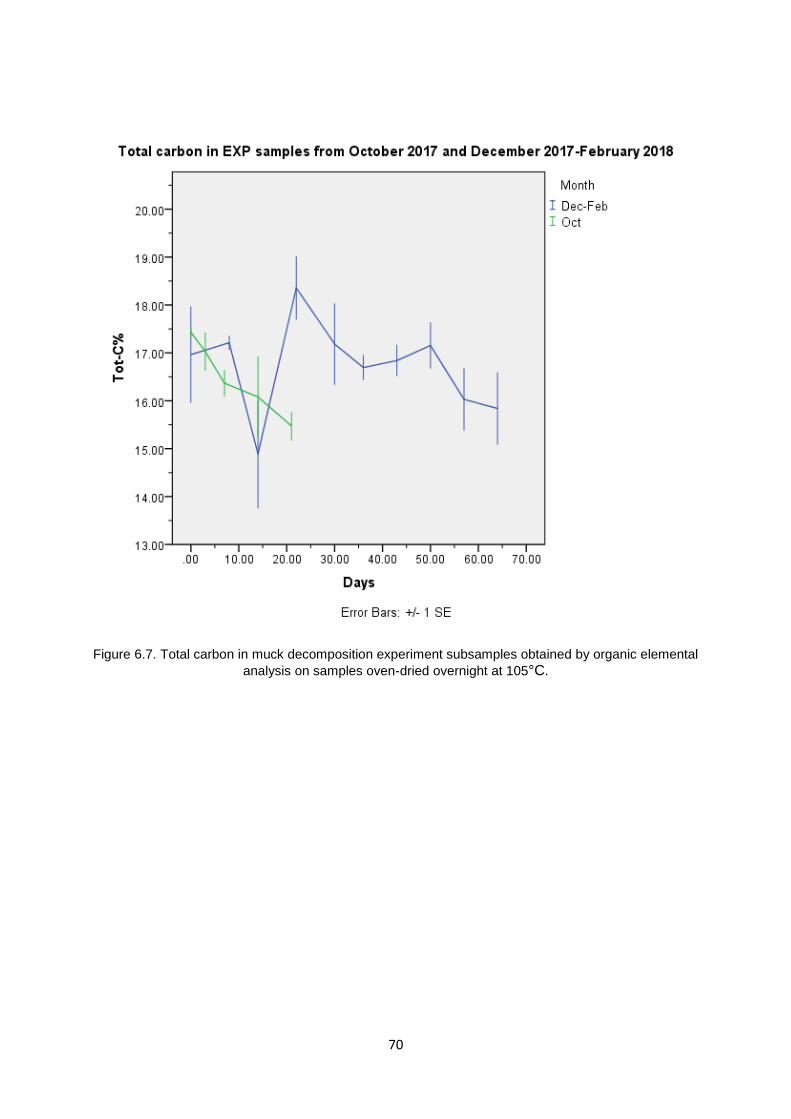
70

Figure 6.7. Total carbon in muck decomposition experiment subsamples obtained by organic elemental

analysis on samples oven-dried overnight at 105°C.

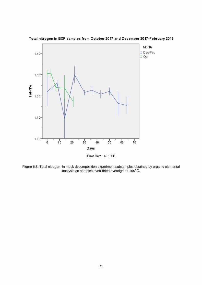
71

Figure 6.8. Total nitrogen in muck decomposition experiment subsamples obtained by organic elemental

analysis on samples oven-dried overnight at 105°C.

72

Figure 6.9. Climatological data for Xochimilco, Mexico. Source: dmi.dk

6.6.2 Nitrate and Ammonium in EXP Samples

Nitrate and ammonium concentrations provide more detail in the decomposition process of organic

material in the October run of the muck decomposition experiment (Fig. 6.10).

It is quite visible that the lake sediment initially contains relatively large amounts of ammonium, but

very little nitrate.

Once moved into an aerobic environment, however, ammonium is rapidly used up. After the first

week of decomposition, a surplus of nitrate in solution can be observed, eventually reaching as high

as 30 mg/kg wet weight. This excess nitrate amounts to about 30 mg/kg, or 6.78 mg-N/kg, after 21

days of decomposition, between one fifth and one tenth of the labile nitrogen added to a local soil in

conventional agriculture of maize and wheat by Patiño-Zúñiga et al. (2009). In terms of mass, this

represents a net mobilization of 0.05% of the sediment’s total nitrogen.

It is worth noting that there is nothing indicating that the starting ammonium is lost to leaching during

the first three days in which excess water drained out from the samples, as far most of the observed

loss occurred after 7 days of exposure to aerobic conditions.

73

Figure 6.10. Nitrate and ammonium in samples from the muck decomposition experiment run in October 2017. Concentrations are wet weight.

6.6.3 Total, Inorganic and Labile (Olsen) Phosphorus in EXP Samples

The different fractions of phosphorus in the muck decomposition experiment show an interesting

picture (Fig 6.11). While the total amount of phosphorus remains largely constant, indicating little to

no loss to leaching as excess water drained from the sediment samples, the inorganic fraction of

phosphorus increased noticeably in the 21 days that the October run lasted.

This mineralization is, however, not followed by an equal increase in the labile phosphorus as

determined by the Olsen extraction method, which remains fairly constant throughout the experiment

(Fig. 6.12).

74

Fig 6.11. Total, inorganic and Olsen phosphorus in samples from the muck decomposition experiment run in October 2017. Total and inorganic phosphorus were extracted using 6M H2SO4 in a 70°C sand bath, with

and without without previous calcination at 550°C, respectively.

75

Figure 6.12. Detail of the Olsen phosphorus measurements from the muck decomposition experiment run in October 2017.

76

7. Discussion

The environmental changes outlined in Chapter 4, together with the results presented in Chapter 6

make clear the need to adapt the theoretical ecosystem ecologies of carbon, nitrogen and

phosphorus constructed in Chapter 3.

The logical place to start is to modify the morphological model to fit both the current state of the lake

and the soil characteristics observed in the field, particularly in terms of the organic matter content

of the soil, its bulk density and the hydrological regime it is subjected to at different depths. Since it

is at the HS chinampa most field data was collected, we’ll modify our model according mostly to its

morphology, using data from the SW1 to provide extra detail. It should be mentioned that based on

observations made on the field, the HS location is representative of the extant Xochimilco chinampas

in terms of height and dimensions.

Figure 7.1. Dimensions of the HS field. Notice that the location seems to be composed of several chinampa beds.

77

The HS chinampa is irregular in shape, but it is visible that it was built with a rectangular shape in

mind (Fig. 7.1). Judging by the placing of secondary canals and changes in vegetation, it is likely

that the HS location is in reality an incomplete amalgam of several smaller raised beds. The entire

location is close to 30 m wide and 100 long, with a secondary canal dividing the front-right quadrant

almost perfectly. Another secondary canal seems to continue at the back half of the location, dividing

the back-left quadrant, belonging to Humedalia A.C., from the back-right quadrant, which is currently

abandoned. Thus, it seems the physical size of the fields that make up the HS location is rather 15

m in width and 50 m in depth, a five-fold increase in area from our initial model.

Measurements from 2012 (Contreras Ruiz Esparza, 2012) put the mean canal water levels in the

rainy and dry seasons at 0.95 to 1.22 m deep, respectively, suggesting that the extant chinampas of

Xochimilco are a good deal taller than previously modelled. In the particular case of the HS site, the

depth of the nearby canals varies from 0.93 m in the dry season (from sampling in January-February)

to 0.55 m in the rainy season (from sampling in July-September). The depth in the canals

immediately surrounding the HS chinampa is not known precisely, but based on observations made

during the fieldwork of this thesis, these canals do seem to have a depth of approximately 0.5 m by

the end of the rainy season.

The surface of the fields at the HS location was close to 1.3 m above the water level during the

fieldwork in September 2017. Thus, given the depth of the modern lake, a height of 1.3 m from the

water at the end of the rainy season puts the height of the HS chinampa from its base at 1.8 m, over

half a meter taller than previously modelled. Whether this height corresponds to the original

construction of the HS chinampa or is the result of centuries of added material, is unknown.

Putting the previous observations together, we have a chinampa that is 1.8 tall from the bottom of

the canals. The bottom 50 cm are permanently saturated, and the top 90 cm are permanently above

the water table. A layer of 40 cm between these two is seasonally inundated, with the highest level

of the water table during the dry winter months and the lowest during the rainy summer months.

The opposition of the lake stage to the seasonal rains reflects the level to which the local hydrology

has been transformed by the surrounding city, as most of the water in the lake originates in sewage

treatment facilities, and the flow into the lake is likely reduced during the rainy season as a precaution

against sudden heavy rainfall.

78

From the field measurements taken at the Humedalia A.C. chinampa, it is immediately apparent that

modern chinampas are heavier than we considered in our initial model (Fig. 6.2). Whether this is the

result of centuries of organic matter decomposition, the retreat of the capillary zone due to failing

water levels in the lake or both, is uncertain. From the deeper bulk density samples taken at sites

HS1 and HS4, however, it seems that the bulk density of the main body of the Humedalia A.C.

chinampa is closer to 0.6 ton/m3, still a light material compared to more mineral soils, but heavier

than the theoretical value used for wetland soils in Chapter 3.

The effects of use and management are most visible on the upper 30 com of the soil, where the

topsoil at plant nursery site, HS1, is nearly half as dense as in the bare soil of site HS4, which is

constantly walked on. Not shown in Figure 6.2 is the topsoil bulk density measurement taken at the

active bed, HS2, which has a value of 0.35 ton/m3, similar to that of the plant nursery soil.

The chinampa’s hydrology also plays an important role in the compaction of the soil, as can be seen

in the low-lying site SW1. There, the bulk density in the unsaturated soil (upper 40 cm in September)

is closer to what we expected from a wetland soil and does not change very drastically throughout

the first 30 cm as the drier soils of HS1 did.

In general, it can be expected that taller, drier chinampas are more compact, with bulk densities in

the main body of up to 0.6 ton/m3 and steeper density gradients in the upper 30-40 cm, while lower

chinampas remain lighter and more homogeneous, likely due to the presence of a high water table.

Furthermore, density seems to be negatively related to soil organic matter content, as the lowest

density value at the surface of HS1 correspond to the highest SOM content of 31%, and the highest

soil density in HS4 corresponds to a SOM content of 14.4%.

These results are interestingly different from those found by Krasilnikov et al. (2011) in Xochimilco,

where bulk density was highest, 0.8 ton/m3, at the surface and decreased steadily with depth to

approximately 0.4 ton/m3 approximately 1 m below the surface; and no correlation between density

and SOM can be seen.

Considering the bulk density of the SW1 soil below the 15 cm affected by ploughing, it seems that

chinampa material under wetter conditions retains a bulk density in the range of 0.45 - 0.5 ton/m3.

Therefore, the higher density of the soils from HS1 and HS4 at similar depths likely stems from a

higher degree of decomposition due to the lower water table relative to the soil surface in these sites.

79

Clearly, there is no evidence of organic matter contents as high as we assumed for the top of a well-

amended chinampa soil (60% SOM as mentioned by Robertson (1983)), with a measured average

SOM in HS1 of 19%. This corresponds to a carbon content of barely 9.5%, just under half of the

theoretical value used in the model in Chapter 3. Even considering the SOM contents of HS1 at 0

cm and SW1 at 25 cm, thinking of a chinampa with a shallow water table regularly amended with

lake sediment, the average value for SOM is 25%, with a corresponding carbon content of 12.5%.

Comparing the different measurements made by Krasilnikov et al. (2011) and those made in this

thesis it is easy to see that the bulk density profiles of extant chinampa soils can vary rather

unpredictably, likely a result of the great diversity of construction methods and materials in the

Chinampa tradition. In order to continue, however, we will need to make some approximations and

assume that changes throughout the soil profile are relatively smooth and linear, allowing for

calculations to be made using average values.

Thus, we can update our model chinampa considering an agricultural soil with a bulk density

gradually increasing from 0.35 ton/m3 to 0.6 ton/m3 between 0 and 30 cm of depth (the range outside

of the capillary fringe), then gradually decreasing from 0.6 ton/m3 to 0.45 ton/m3 throughout the

capillary fringe to a depth of 0.9 m, and then retaining a density of 0.45 ton/m3 in all of the seasonally

and permanently inundated material down to the base at 1.8 m below the surface.

This leaves us with a soil composed of a 30 cm topsoil layer with an average density of 0.475 ton/m3,

and a mass of 1,425 ton/ha. The following 60 cm would have an average bulk density of 0.525 ton/m3

and a mass of 3,150 ton/ha. Finally, the bottom 90 cm of the chinampa, made up of an upper 40 cm

that is seasonally inundated and a bottom 50 cm permanently saturated, would have a constant bulk

density of 0.45 ton/m3, giving it a mass of 4,050 ton/ha (Fig 7.2).

Thus, the total areal mass of the chinampa soil adds up to 8,625 ton/ha. Estimating that 25% of the

remaining 2,215 ha of Chinampa landscape is taken up by the canals (Luna Goyla, 2014; GIAHS),

this amounts to a total of 14,3 million tonnes of moved soil in the surviving chinampa beds.

80

Figure 7.2. Extant chinampa morphology based on the HS location from this thesis’ fieldwork.

Carbon, nitrogen and phosphorus pools in the soil have shown as well to be more complex than

previously modelled, while many if not all the main fluxes in the system have been altered by the

environmental changes discussed before.

The SOM measurements made in bulk density ring samples would suggest that most variation in

soil carbon occurs in the upper 40 cm. However, total carbon and total nitrogen measurements from

organic elemental analysis in soil core samples show a much more diverse picture of the Chinampa

soil. These total carbon and nitrogen profiles offer perhaps the best glimpse into the construction of

the Humedalia A.C chinampa, as well as the broad strokes of the main processes in action within

the soil.

The total soil carbon content at the surface is indeed different for each site, ranging from just under

7% at HS2 to over 17.5% at HS1. Total soil nitrogen, being primarily composed of organic nitrogen,

follows the same patterns as carbon ranging from 0.5% at HS2 to 1.2% at HS1. This reflects quite

clearly the effects management and plant cover. Increased aeration from ploughing and somewhat

81

drier conditions clearly have promoted mineralization of carbon and nitrogen in in the surface of HS2,

while the lack of tilling and constant mucking also have visibly added large amounts of organic matter

to the topsoil of HS1, while, perhaps due to the intense root growth of lawn grass, SOM seems to

also accumulate near the surface at HS3. On the other hand, the less modified soils, HS4, HS5 and

SW1, all show surface total carbon and nitrogen contents of almost exactly 8% and 0.6%,

respectively, indicating that this is likely the natural state of the chinampa material at the surface in

modern times.

Phosphorus, on the other hand, seems to be largely independent from SOM. Judging by the fact that

HS1, HS2, HS3 and HS4 have all nearly equal total phosphorus concentrations at the surface, lower

than that of HS5 and considerably lower than that of SW1, soil phosphorus seems to be more related

to the addition of plant material (unremoved litter in HS5 and green manure in SW1) than to SOM.

Interestingly, even though the lake sediment used for mucking is relatively high on phosphorus,

between 2.4 and 2.6 mg-P/g, only about than a third of this concentration could be found at or near

the surface of HS1.

Other than faulty quantification, the only explanation for this is a rapid removal of phosphorus during

the first few weeks of plant growth in the nursery beds, highlighting the importance of the almárcigo

in the traditional practice.

Beyond the superficial differences, however, there are visible features that are shared by several or

all profiles at greater depths. One of these features, as mentioned in Chapter 6, is the region of high

carbon and nitrogen concentrations between 70 and 85 cm of depth. In the HS sites, this area

coincides roughly with both the maximum height of the lake stage in the dry season (90 cm from the

surface) and with the maximum height of the capillary fringe in the wet season (70 cm from the

surface), if we assume a capillary rise of 60 cm as in Chapter 3. However, this feature is also present

in SW1, even though the water table there is a good deal higher. Therefore, it is likely not due to a

change in the soil’s hydric regime with depth or a prevailing downward movement of dissolved

organic material that these areas of accumulation have formed.

This area accumulation on the other hand, is completely absent from the phosphorus profiles,

suggesting that it stems from a concentration of SOM independent from the processes that mobilize

and deposit phosphorus minerals. The C:P ratios of the different profiles confirm this, with the

exception of HS1, which shows a conspicuous depletion of phosphorus as depth increases, reaching

C:P ratios above 400 at the same depths as the SOM accumulation region (Figure 7.3).

82

Figure 7.3. C:P ratios from the mean concentrations of total carbon by organic elemental analysis and

phosphorus by ICP-MS.

It is possible that this area high SOM corresponds to peaty substrates originating in the use of plant

material for construction. Its position in respect to the surface certainly fits with the model of a

complex chinampa with a plant based foundation presented before, where mats of plant material

would provide extra cohesion for the added mud or soil in the first stages of construction in standing

water, and then overlaid with roughly one meter of muck or imported dryland soil and possibly more

plant material. However, this theory places the foundation of the SW chinampa a good 40 cm below

the water level of the modern lake in the rainy season, while at the same time placing the foundation

of the HS chinampa at 50 cm above the water level of its own canals in the same season. It is

possible that this difference stems from the sinking of the SW chinampa, or from the HS chinampa

being taller and more complex than our model, with several thick layers of plant-rich material in its

profile. It is also possible that the HS chinampa was constructed at a time where the lake was half a

meter deeper, and that the construction of the SW chinampa, as well as of those around it, occurred

83

later, after the lake stage had decreased considerably. The problematic aspect of all these

explanations is that their confirmation or rejection would require a serious archaeological excavation

and the dating of carbon sediments and artefacts from the profile, which is sadly not available for

either of our locations. This type of investigation has indeed been performed in a multitude of extant

and buried chinampas across the Xochimilco-Chalco region, but due to the long and chaotic history

of Chinampa agriculture, even nearby chinampa fields can be centuries apart in age. Without any a

priori knowledge of the age of these chinampas, or the state of the lake at the time of their

construction, it is unfortunately futile to look to other profiles for answers.

An alternative explanation worth considering is that this accumulation of SOM stems rather from

decomposing root fragments of the ahuejote trees that line (or used to line) the edges of both the

SW and the HS chinampas. Indeed, total carbon and nitrogen concentrations at this depth are

highest in SW1 and HS1, which are also the sites closest to existing treelines. This would also explain

why the accumulation zones are much less prominent in HS4 and HS5, and are completely absent

in HS2 and HS3, given that the Salix trees near all these sites have been removed. Furthermore,

this would imply that the practice of planting trees along the edges of the chinampas, besides

providing shade, stopping the wind and contributing to a milder microclimate, also played an

important role in the soil’s carbon and nitrogen cycles, adding between 0.5% to 7% in total carbon

and 0.07% to 0.4% in total nitrogen by mass to the pre-existing soil matrix.

This explanation, however, requires the species Salix bonplandiana to be capable of growing dense

roots into the waterlogged soil of SW1 to nearly the same depth as it would into the capillary fringe

of HS1. To grow deep roots regardless of water saturation is a property of the ahuejote tree that is

indeed part of the traditional system of beliefs, but for which there is no actual empirical information.

Wilken (1986) remaked upon this precise point, where he questioned the common belief in ahuejote

roots being able to anchor a chinampa to the lake floor is nearly universal in spite of there being no

evidence that they could penetrate that far below the water table. The Mexican environmental

authority (Salix bonplandiana, 2018), however, does describe the species Salix bonplandiana as a

tree native to wetland and mangrove environments, adapted to elevated salinities and capable of

growing in very wet to inundated soils under the influence of both marine and freshwater bodies.

Thus, it is not entirely impossible that the rhizosphere of the ahuejote tree in fact reaches deep and

far into the Chinampa soil, depositing large amounts of organic material in the process.

Another more superficial zone of SOM accumulation is visible in several profiles between 15 and 40

cm of depth. Interestingly, the three sites where this zone is most visible are HS2, at around 15 cm

84

of depth, HS1, at 35 cm, and HS4, between 20 and 30 cm below the surface. It is possible that these

accumulation zones also correspond to local rhizospheres, however, in HS1 most of the plantules

are removed before their roots outgrow the mud plugs that contain them, and HS4 is kept clear from

vegetation due to its role as access point for irrigation.

Alternatively, these regions of accumulation could originate in leached organic material from the

topsoil, forming at different depths due to rain and irrigation water penetrating more or less into the

soil. Site HS1, being the plant nursery, would be very thoroughly irrigated yet kept mostly bare except

for developing seeds and plantules for most of the year, allowing for high rates of percolation. These

conditions, together with constant mucking, would explain the relatively deep and strong

accumulation of organic material seen in the carbon and nitrogen profiles. HS4 is also bare, but

much more compact than the soils under use, particularly at 40 cm and below. Thus, organic material

leached down by unintentional irrigation and by the summer rains would accumulate on top of the

compact soil at 40 cm of depth. HS2 also receives plenty of irrigation, while at the same time the soil

is constantly ploughed and mixed. Thus, although SOM can easily leach down from the light and

rapidly decomposing topsoil, it has had little time to since the last turning, and thus creates a shallow

and less conspicuous accumulation zone. Indeed, this could also be the case in SW1, although the

peaks in its total carbon and nitrogen profiles are much smaller and less well-defined. On the other

hand, the lawn in HS3 and the wild plant cover in HS5 very likely intercept and absorb most of the

water that these soils receive from rain and, in the case of HS3 only, irrigation; leaving little

percolation to carry dissolved materials down, preventing the formation of SOM accumulation zones

deeper in their profiles.

Indeed, the phosphorus profile at HS3 shows a very visible decrease in phosphorus concentration

at 10 cm of depth, perhaps the only distinct feature among the HS phosphorus profiles. This localized

phosphorus depletion supports the idea of a very high degree of soil water interception and nutrient

uptake by the dense roots of the lawn grass.

Thus, based on the measurements obtained in Ring and Core samples, and the mechanisms

discussed above, we can begin to build a more complex ecosystem ecology of carbon, nitrogen and

phosphorus in a modern chinampa as described by our new morphological model, starting with the

carbon, nitrogen and phosphorus pools in the soil. Diagrams summarizing the ecosystem ecologies

of these three elements as discussed at length in the following pages are shown in Figures 7.7, 7.8

and 7.9 at the end of this chapter.

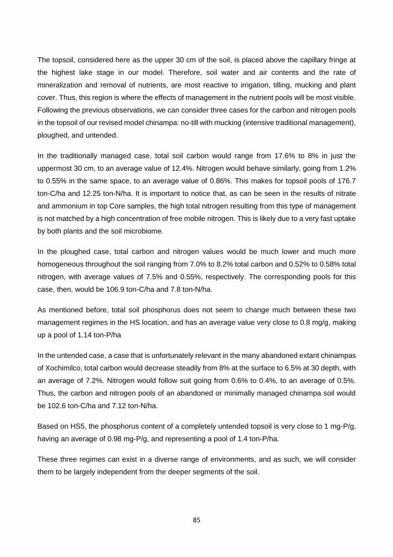
85

The topsoil, considered here as the upper 30 cm of the soil, is placed above the capillary fringe at

the highest lake stage in our model. Therefore, soil water and air contents and the rate of

mineralization and removal of nutrients, are most reactive to irrigation, tilling, mucking and plant

cover. Thus, this region is where the effects of management in the nutrient pools will be most visible.

Following the previous observations, we can consider three cases for the carbon and nitrogen pools

in the topsoil of our revised model chinampa: no-till with mucking (intensive traditional management),

ploughed, and untended.

In the traditionally managed case, total soil carbon would range from 17.6% to 8% in just the

uppermost 30 cm, to an average value of 12.4%. Nitrogen would behave similarly, going from 1.2%

to 0.55% in the same space, to an average value of 0.86%. This makes for topsoil pools of 176.7

ton-C/ha and 12.25 ton-N/ha. It is important to notice that, as can be seen in the results of nitrate

and ammonium in top Core samples, the high total nitrogen resulting from this type of management

is not matched by a high concentration of free mobile nitrogen. This is likely due to a very fast uptake

by both plants and the soil microbiome.

In the ploughed case, total carbon and nitrogen values would be much lower and much more

homogeneous throughout the soil ranging from 7.0% to 8.2% total carbon and 0.52% to 0.58% total

nitrogen, with average values of 7.5% and 0.55%, respectively. The corresponding pools for this

case, then, would be 106.9 ton-C/ha and 7.8 ton-N/ha.

As mentioned before, total soil phosphorus does not seem to change much between these two

management regimes in the HS location, and has an average value very close to 0.8 mg/g, making

up a pool of 1.14 ton-P/ha

In the untended case, a case that is unfortunately relevant in the many abandoned extant chinampas

of Xochimilco, total carbon would decrease steadily from 8% at the surface to 6.5% at 30 depth, with

an average of 7.2%. Nitrogen would follow suit going from 0.6% to 0.4%, to an average of 0.5%.

Thus, the carbon and nitrogen pools of an abandoned or minimally managed chinampa soil would

be 102.6 ton-C/ha and 7.12 ton-N/ha.

Based on HS5, the phosphorus content of a completely untended topsoil is very close to 1 mg-P/g,

having an average of 0.98 mg-P/g, and representing a pool of 1.4 ton-P/ha.

These three regimes can exist in a diverse range of environments, and as such, we will consider

them to be largely independent from the deeper segments of the soil.

86

In the following 40 cm of the profile, the portion where soil water is dominated by capillary rise from

the water table during the dry season but dominated by rain and irrigation water during the rainy

season, we will consider the two extreme cases in terms of plant cover and movement of dissolved

nutrients with percolating water: year-round plant cover capable of intercepting nearly all water at

the topsoil, and completely bare soil with strong percolation of dissolved organic material.

In the first of the two cases, where all or most rain and irrigation water is stopped at the surface, no

organic material is deposited through percolation, and the soil carbon and nitrogen content is

affected only by the relatively slow effect of decomposition and capillary movement during high water

tables. This case corresponds to what was observed in HS3 and HS5, one with constant cover of

lawn and the other in wild plants. Here, total carbon contents vary very little with depth, keeping

values between 6% and 6.5%. Total nitrogen behaves similarly, keeping values between 0.38 and

0.46. Therefore, we will consider an average soil carbon value of 6.25% and an average nitrogen

value of 0.42%, which makes up pools of 130 ton-C/ha and 8.7 ton-N/ha.

The second case at this depth corresponds to bare soils with high degrees of percolation and

leaching of organic material from the surface, such as HS1 and HS4. Here, accumulation of SOM

leads to point total carbon contents of 9.8% and 10.4%, with an average of 8.5%; and total nitrogen

contents as high as 0.7%, and an average of 0.55%. These concentrations lead to larger pools of

177 ton-C/ha and 11.4 ton-N/ha.

The 20 cm below correspond to the portion of the soil below the maximum reach of the capillary

fringe during the low water table in the rainy season, and above the high water table during the dry

season. It is here that we can expect the bulk of the water-resistant roots of ahuejote trees to grow,

and thus it is here where we would see the second area of SOM accumulation. We will therefore

consider two cases, where nearby trees are either present or absent, analogous to the profiles of

HS1 and SW1, and HS2 and HS3, respectively.

In the case where nearby ahuejote trees are present, the soil between 70 and 90 cm of depth would

present a strong localized increase in SOM, reaching maximum total carbon values between 14%

and 15.3%, and total nitrogen values between 0.86% and 0.96%, respectively. Taking average

values in this narrow region, we get a total carbon content of 12.75% and a total nitrogen content of

0.80%, with corresponding pools of 132 ton-C/ha and 8.3 ton-N/ha.

In the case with no nearby ahuejotes, there would be no deposition of organic matter from tree roots

in the bottom 20 cm of the first meter of the profile, which would leave the background carbon and

nitrogen contents, respectively 7.0% - 8.0% and 0.37% - 0.67%, unaffected. The average values

87

we’ll consider for this narrow band, then, will be 8% for total carbon, and 0.55% for nitrogen, with

corresponding pools of 72 ton-C/ha and 5 ton-N/ha.

Phosphorus behaves differently than carbon and nitrogen in the lower 70 cm of the extracted cores,

where it decreases steadily at all sites from a mean of 0.85 mg-P/g at 35 cm depth, to a mean of 0.4

mg-P/g at 85 cm depth, with relatively little difference among HS sites at equal depths. There appears

to be the start of an increase in total phosphorus in the bottom 5 or 10 cm of the profiles, reaching

nearly 0.9 mg-P/g in HS2 starting at 95 cm of depth, with a mean concentration among bottom HS

samples (90 and 95 cm) of 0.67 mg-P/g. Unfortunately, since this increase in concentration can only

be seen at the very bottom of some of the HS profiles, it is impossible to know whether it corresponds

to an area of accumulation, or a steady rise in values reaching far into the soil. For this reason, these

values will not be considered in the phosphorus pool at this point. Thus, we will consider the region

between 30 and 90 cm of depth to have an average phosphorus concentration of 0.625 mg-P/g,

which makes up a phosphorus pool of 1.95 ton-P/ha.

Finally, since we have no first-hand data for the composition of our chinampas below 90 cm of depth,

we will need to use data from other sources. Crossley (1999) performed excavations in several

chinampas in Xochimilco, Mixquic and the Chalco region, and found that the organic matter content

below 1 m of depth ranged from as low as 4% in volcanic ash-rich deposits to nearly 60% in layers

of peaty material, with no common general pattern among sites. This, once again, is due to the great

diversity among chinampa construction methods, times of construction, and the many modifications

made to their soils since the Spanish Conquest. However, using averages of the SOM content in

strata below 1 m of depth found by Crossley weighed for the thickness of each stratum, we obtain

SOM values at his four deepest sites between 20% and 30%. That means between 10% to 15%

organic carbon, of which we’ll take 12.5% as an estimate for the average carbon content in the very

diverse matrix of the lower part of our model modern chinampa. This, with an overall bulk density of

0.45 ton/m3, gives us a very general carbon pool of 506.25 ton-C/ha for all material below 90 cm of

depth in a Xochimilco-Chalco chinampa.

Likewise, the available phosphorus measured in those same samples varies between as little as 11

ppm to over 200 ppm, and can easily increase and decrease five-fold within the same profile.

Average concentrations weighed for stratum thickness vary as well between 41 ppm and 173 ppm

between profiles, with an overall mean of 95.7 ppm. Since available phosphorus can make up as

little as 10% of the total phosphorus in soil, we can give the lower 90 cm of our model chinampa a

conservative total phosphorus concentration of 957 ppm, or 0.96 mg-P/g, giving us a pool of 3.9 ton-

P/ha.

88

Total nitrogen was not quantified by Crossley or in any other available investigation at depths below

90 cm, so we need to estimate it indirectly. In the samples analysed in this thesis, the C:N ratio of

the soil occupies a range between 12.5 and 19, with a slight tendency to increase with depth (Figs

7.4 and 7.5). This gradual decrease of nitrogen relative to carbon likely reflects the predominantly

anoxic environment encountered deeper in the soil, where respiration is slow or null. Thus, we will

take the maximum measured C:N ratio of 19 for the lower half of the chinampa, giving us a nitrogen

content of 0.65% and a total nitrogen pool of 26.32 ton-N/ha.

Figure 7.4: C:N ratio of Core samples by site and depth.

89

Figure 7.5: Average C:N ratio of all Core samples by depth.

Having calculated the soil carbon, nitrogen and phosphorus pools in our model modern Xochimilco

chinampa, we can move on to modify the flows according to field measurements as well as modern

sources.

We’ll begin, as before, with primary productivity on the soil environment. According to the Mexican

national hydrological authority (CONAGUA, 2015) the mean yearly potential evapotranspiration for

the central Basin is 1558.8 mm. This value is over three times larger than the one calculated by

Robertson (1983) and used in Chapter 3 for the model prehispanic chinampa, likely due to the nearly

complete deforestation of the basin and the “heat island” effect from the surrounding city.

Expecting the modern farmer to keep up with all the water needs of the crops to a degree where we

can consider potential evapotranspiration equal to actual evapotranspiration is a tricky proposition.

Not only does the farmer in our model modern chinampa not have the support of the lake for

subirrigation due to the recession of the capillary fringe, but mean annual precipitation only accounts

only for 768.5 mm, leaving over half of the yearly PET to be supplied by irrigation with the saline,

nutrient-rich and potentially contaminated lake water. Nevertheless, let us suppose that with the help

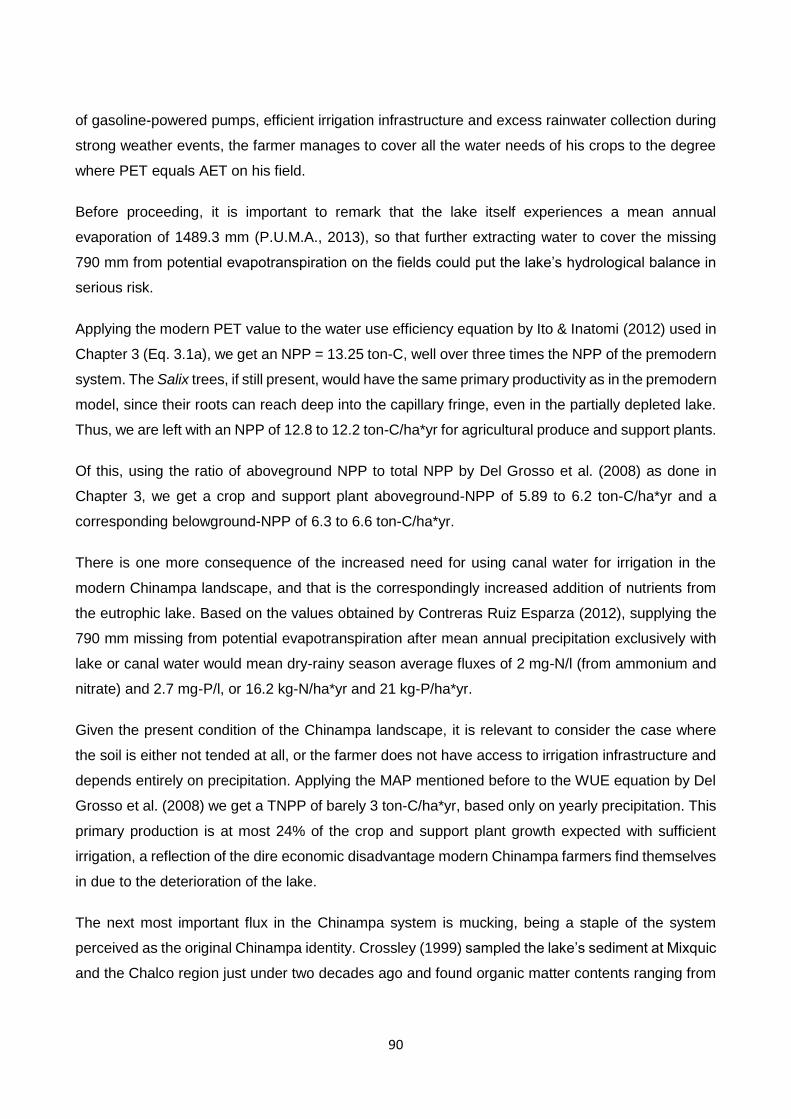
90

of gasoline-powered pumps, efficient irrigation infrastructure and excess rainwater collection during

strong weather events, the farmer manages to cover all the water needs of his crops to the degree

where PET equals AET on his field.

Before proceeding, it is important to remark that the lake itself experiences a mean annual

evaporation of 1489.3 mm (P.U.M.A., 2013), so that further extracting water to cover the missing

790 mm from potential evapotranspiration on the fields could put the lake’s hydrological balance in

serious risk.

Applying the modern PET value to the water use efficiency equation by Ito & Inatomi (2012) used in

Chapter 3 (Eq. 3.1a), we get an NPP = 13.25 ton-C, well over three times the NPP of the premodern

system. The Salix trees, if still present, would have the same primary productivity as in the premodern

model, since their roots can reach deep into the capillary fringe, even in the partially depleted lake.

Thus, we are left with an NPP of 12.8 to 12.2 ton-C/ha*yr for agricultural produce and support plants.

Of this, using the ratio of aboveground NPP to total NPP by Del Grosso et al. (2008) as done in

Chapter 3, we get a crop and support plant aboveground-NPP of 5.89 to 6.2 ton-C/ha*yr and a

corresponding belowground-NPP of 6.3 to 6.6 ton-C/ha*yr.

There is one more consequence of the increased need for using canal water for irrigation in the

modern Chinampa landscape, and that is the correspondingly increased addition of nutrients from

the eutrophic lake. Based on the values obtained by Contreras Ruiz Esparza (2012), supplying the

790 mm missing from potential evapotranspiration after mean annual precipitation exclusively with

lake or canal water would mean dry-rainy season average fluxes of 2 mg-N/l (from ammonium and

nitrate) and 2.7 mg-P/l, or 16.2 kg-N/ha*yr and 21 kg-P/ha*yr.

Given the present condition of the Chinampa landscape, it is relevant to consider the case where

the soil is either not tended at all, or the farmer does not have access to irrigation infrastructure and

depends entirely on precipitation. Applying the MAP mentioned before to the WUE equation by Del

Grosso et al. (2008) we get a TNPP of barely 3 ton-C/ha*yr, based only on yearly precipitation. This

primary production is at most 24% of the crop and support plant growth expected with sufficient

irrigation, a reflection of the dire economic disadvantage modern Chinampa farmers find themselves

in due to the deterioration of the lake.

The next most important flux in the Chinampa system is mucking, being a staple of the system

perceived as the original Chinampa identity. Crossley (1999) sampled the lake’s sediment at Mixquic

and the Chalco region just under two decades ago and found organic matter contents ranging from

91

18% to 32%, with an average among nine sites of 23.3%, and a mean available phosphorus

concentration of 293 ppm. Keeping in mind that available phosphorus makes up only around 10% of

the total soil phosphorus, this corresponds to an organic carbon content of 11.6% and a total

phosphorus content of 2.94 mg-P/g.

The total carbon content measured in EXP samples was somewhat higher, with an average value of

17.4% in October and 17.0% in December 2017, while the total phosphorus concentration was lower,

with a mean value of 2.35 mg-P/g. This difference is likely due to the fact that the EXP samples do

not come from a random sampling of the lake’s sediment, but from muck specifically selected for its

high organic content to be used in the almárcigo nursery, and that the main portion of the phosphorus

in the Chinampa environment is not a part of the organic material. For this reason, we will consider

a total carbon content of 17%, just over half of what was considered in the premodern model, and a

total phosphorus concentration of 2.35 mg-P/g in the sediment used for mucking.

Thus, having a mucking layer of 5 cm as before, and a bulk density of moist (not wet), recently laid

sediment of 0.3 ton/m3 like the surface of HS1, every round of mucking represents a carbon flow of

25.5 ton-C/ha. Even with a lighter material and a much lower carbon content than in the premodern

model, these calculations show that mucking every year still exceeds what one would expect from

even a highly productive lake environment.

The solution is, as before, mucking at a lower frequency. This is accomplished often by mucking

once or twice a year, but only over a portion of the field at each time, as Sanders proposed (1993 in

Crossley, 1999). By mucking twice a year and covering one tenth of our model chinampa at a time,

we can accomplish a mucking frequency equivalent to one complete mucking every five years, the

same low frequency we chose in Chapter 3. This would represent a mean yearly carbon flow of 5.1

ton-C/ha*yr.

The effect of mucking on the lake’s carbon budget is difficult to estimate without an idea of its primary

productivity and inputs from surface runoff, but the increase in plot size that occurred after the

Spanish conquest certainly exacerbates the effects of extracting sediment from the canals to boost

soil fertility. Our model modern chinampa, being 15 m wide and 50 m2 long, is surrounded by 260

m2 of canals considering an average canal width of 2 m. In order to provide the 2.25 ton of sediment

per year required to muck the entire chinampa every five years, the net primary production in the

canals would have to be at least 1.5 kg-C/m2*yr. A smaller field such as the premodern model

chinampa outlined in Chapter 3, however, would only extract 450 kg of sediment per year,

corresponding to 0.36 kg-C/m2*yr, from its surrounding 212 m2 worth of canals. Thus, the larger size

92

of the extant fields is by itself a technological departure from the system conceived as the original

Chinampa agriculture.

In the case of the nitrogen flux from mucking, EXP samples had a mean starting total nitrogen

concentration of 1.3% in October 2017 and 1.22% in December 2017, 1.26% averaged between the

two. This means that at a mucking frequency of 5 cm every five years, nitrogen flows from the canals

into the soil at a rate of 0.38 ton-N/ha*yr. Compared to the nitrogen influx of 50 kg-N/ha*yr estimated

in Chapter 3, this seems like a tremendous excess of nitrogen. However, the vast majority of this

nitrogen is completely inaccessible to plants, requiring first the decomposition of the organic material

of which it forms part. Making back-of-the-envelope extrapolation of the excess nitrate production

rate observed in EXP samples from October (30 mgNO3/kg after 21 days) for a whole year of

decomposition, we get a yearly production of 521 mg of excess nitrate per kg of sediment. Multiplied

by the 30 ton of sediment per hectare per year equivalent to one full mucking every five years, this

yields an addition from muck decomposition of 15.6 kg of nitrate, about a third of the 50 kg-N/ha*yr

that Knapp & Denevan (1986) estimated for sustaining high yields under intensive small-scale

agriculture, and about 1 kg less than the reactive nitrogen added through irrigation.

As for phosphorus, given a mucking frequency of 5 cm over the entire field every 5 years with a total

sediment phosphorus concentration of 2.35 mg-P/g, gives an annual flux of 70.5 kg-P, a little over

three time more than what is transferred through irrigation, but in a much less labile form.

As mentioned in Chapter 4, only a small portion of the extant chinampas still under active agricultural

production use mucking in such a large scale. Many muck only their almárcigos, and an increasing

majority of the surviving farmers apply manure and commercial fertilizers whenever they can afford

it. The fluxes associated to the two modern amendments are impossible to calculate, since the

frequency and magnitude of application varies from farmer to farmer, given that many have little to

no preparation in the use of these resources. However, we can attempt to calculate the flux resulting

from only mucking for the nursery beds, as done in the HS location (Fig. 7.6).

93

Figure 7.6: Newly laid almárcigo nursery being prepared for sprouting of broad beans and other various crops at the HS1 site. The mud has already been cut into square plugs, or chapines and seeds have been

placed in them by hand, one by one.

At a planting density of 6 plants per square meter, corresponding to local modern intensive maize

agriculture (Patiño-Zúñiga et al., 2009), and a chapín plug roughly 5 cm by side, every hectare

planted with maize would require 0.15 ha of almárcigo, or, rather, each hectare of active chinampas

would consist of 0.87 ha of active beds and 0.13 of almárcigo. If the farmer is able to provide irrigation

and care for two harvests per year, this leaves us with a yearly application of 39 ton/ha of lake

sediment in the nursery beds, corresponding to 6.63 ton-C/ha*yr, 0.49 ton-N/ha*yr and 91.6 kg-

P/ha*yr.

94

These fluxes are not all too different from those from covering the entire field over the course of five

years, with the key difference that under this practice, all the applications are made on the same site,

likely in a convenient location close to the edge of the chinampa.

A pertinent observation is that most seeds placed in a nursery bed made of lake sediment sprout

within the first two weeks after seeding. Thus, by the time they develop a rudimentary root system,

excess nitrate is already accumulating in the surrounding soil, available for uptake by the plant. This

makes the use of almárcigo nurseries and the transplantation of sediment plugs an advantageous

technique if properly timed with seeding and bed preparation. On the other hand, judging from the

results of the muck decompositions experiment, much of the mineral phosphorus released from the

lake sediment is quickly immobilized and made it unavailable for plant use. Thus, it is very likely that

the soil after mucking is P-limited, not due to a lack of total phosphorus, but to a relatively low degree

of availability.

The last important nutrient inflow in the modern Chinampa soil is nitrogen fixation. It is logical to

expect that nitrogen fixation is still dominated by symbiotic rhizome bacteria in legumes, so the

choice of crops in the extant fields will determine whether this flux is relevant. Recent data suggests

that most of the active Chinampa farmers left in the Xochimilco area have turned their backs on

traditional crops such as maize, gourd and beans, in favour of faster-growing produce like lettuce,

purslane, brassicas and spinach, among others, as well as ornamental plants and flowers (CDMX-

GOV, 2017; P.U.M.A., 2013). Indeed, according to a 2014 census compiled by the Mexico City

government, the entire chinampa region of Xochimilco-Chalco only produced 40.7 ton of beans that

year, while at the same time achieved yields of 2,660 ton of lettuce, 3,400 ton of broccoli, 1,500 ton

of purslane and as much of 4,500 ton of romeritos (Suaeda torreyana), a native halophile bush used

in Mexican cuisine during the Easter and Christmas holidays.

Thus, given the very small role that beans seem to play in modern Chinampa agriculture, the

symbiotic nitrogen fixation associated with legumes will not be included in their modern ecosystem

ecology.

The outflows of carbon and nutrients in the modern setting are as well difficult to calculate,

particularly those corresponding to harvest, since the productivity of the soil can vary dramatically

from nearly nil to very high depending on a variety of environmental aspects. Water stress, soil

salinity and plagues seem to be the parameters that more strongly determine yields, although there

is also a strong perceived need for nutrient inputs in the shape of manure and mineral fertilizers

among many farmers (P.U.M.A., 2013). However, by dividing the reported 2014 production (15,313

ton) over the area of still active extant chinampas (423.5 ha) we get an overall annual yield of 36.2

95

ton/ha, in spite of the fact that an important portion of the soil is dedicated to floriculture. This number,

however, can go as low as 6.5 ton/ha even with similar work inputs, as is the case with the yields

reported by Humedalia A.C. in their small-scale biointensive operation. Regardless, from the overall

annual yield of 36.2 ton/ha*yr, mostly in the shape of vegetables and greens, and a very general

carbon content in green plant biomass of 40% dry weight and water content of 75% (Brady and Wile,

2008), we get a carbon outflow of 3.6 ton-C/ha*yr, roughly half of the expected aboveground NPP.

Keeping in mind that the produce from the present-day chinampas is mostly vegetables, meaning

that, unlike grains, very little of the plant is left on the fields, this difference likely indicates that the

farmers in the Xochimilco-Chalco area are either incapable of providing sufficient water for their

plants to reach the full productive potential afforded by the climate, or cannot sufficiently remediate

the effects of soil salinity and pests, in spite of all their efforts to adapt to the degraded landscape.

The corresponding calculation for nitrogen and phosphorus can be made by considering the

elemental compositions of lettuce, broccoli and romeritos, which on their own make up about 69%

of the total reported production in the area.

According to López-Berenguer et al. (2007), broccoli leaves have a total nitrogen content of around

0.35 mmol/g, or 5 mg-N/g (fresh weight), and a total phosphorus content of about 0.15 mmol/g, or

4.65 mg-P/g (fresh weight) at a wide range of NaCl concentration in the soil solution. In the case of

lettuce (cultivars Romaine and Iceberg), Hartz et al. (2007) cite recommended total nitrogen and

phosphorus of concentrations in leaves of around 40 mg-N/g and 5 mg-P/g dry weight,

corresponding to 4 mg-N/g and 0.5 mg-P/g fresh weight considering a 90% water content.

It was unfortunately not possible to locate reliable elemental composition data for romeritos in

literature. Considering, thus, only the nutrient contents of lettuce and broccoli and their relative yields,

we get an estimate for the overall concentration of nutrients in harvested vegetables of 4.6 mg-N/g

and 2.85 mg-P/g.

Thus, from an annual yield of 36.2 ton/ha*yr, we get nutrient outflows of 0.166 ton-N/ha*yr and 0.103

ton-P/ha.

Besides removals from harvest, losses to the atmosphere are arguably the most important outflows

in an agroecosystem. Of these, soil respiration is by far the largest outflow by mass, and represents

also a vital process in the mineralization and mobilization of organic nutrients. However, respiration

rates in the soil can vary greatly depending on the soil’s aeration, water content and nutrient

concentration, making it difficult to estimate one flux size in the complex Chinampa landscape.

96

As mentioned in Chapter 3, Ortiz-Cornejo et al. (2015) measured mean daily CO2 emission rates

between 1.5 kg-C/ha*day and 1.65 kg-C/ha*day, in untilled and unamended chinampa soil,

equivalent to 0.6 ton-C/ha*yr. This flux is small compared to the 1% difference in carbon content at

the top 10-15 cm between HS2, and HS4, HS5 and SW1, such that it would take over 16 years for

that respiration rate and no carbon additions whatsoever to create the difference between the

samples untended soils and the active site HS2, which is longer than the time that the HS chinampa

has been active in recent times. Clearly, the increased aeration and addition of nutrients from

compost and manure has accelerated the oxidation of the soil, removing carbon from it faster than

in an untilled and unamended bed. Indeed, Patiño-Zúñiga (2009) and Dendooven et al. (2014)

registered CO2 emissions from untilled fertilized soils in the same region and climate of 7.01 kg-

C/ha*day and 8.9 kg-C/ha*day, respectively, equivalent to 2.56 ton-C/ha*yr and 3.25 ton-C/ha*yr.

These soil respiration rates could conceivably cause a net removal of carbon of 1% in the soil within

3 to 4 years. For comparison, in conventionally tilled soils from the same studies soil respiration rates

were only 6.5 kg-C/ha*day and 9.15 kg-C/ha*day, indicating that nutrient additions to the soil might

play even a greater role in soil respiration than aeration, given local conditions.

Thus, we can consider the lower respiration rates in the untilled Chinampa as those corresponding

to a soil with plant cover but otherwise little to no management, while the higher rates found in

untilled but fertilized dryland soil would correspond to an active Chinampa growing bed, traditional

or ploughed, that receives significant nutrient inputs from amendment and, importantly, from water.

This leaves us with a carbon outflow from respiration in our model chinampa of 0.6 ton-C/ha*yr in

untended soil and an estimated 3 ton-C/ha*yr in active, irrigated and amended soils.

However, in our model modern chinampa not all of the soil is devoted to growing beds. Every total

hectare of soil is shared between active growing beds and almárcigo nurseries mucked with lake

sediment at each sowing, with two sowing times per year. Although they comprise small portions of

the total chinampa area, these soils have a great potential for mineralizing carbon once laid out due

to their very high initial carbon content and high mineral and organic nitrogen and phosphorus

concentrations. According to the total carbon measurements in EXP samples, this material can

oxidize as fast as 0.01% by weight per day in the first month after extraction. This is equivalent to an

outflow of 150 kg-C/ha*day in a soil entirely devoted to nurseries.

The length of time before plantules are transplanted to growing beds varies depending on the crop,

but taking a ballpark of 30 days of residence in the nursery, and the nursery-to-field area ratio of

0.13-to-0.87 used before, each sowing would come with an added outflow of 585 kg-C/ha. Thus, for

every hectare of productive chinampa soil in our model modern chinampa, we must consider an

97

outflow of 2.61 ton-C/ha*yr from the growing beds and an outflow of 1.17 ton-C/hafield*yr from

almárcigo nurseries.

Although not directly considered for our current model, the particular case of SW1 is interesting in

that it seems to have retained much of its original soil carbon in spite of being productive and

receiving regular ploughing. This would indicate that green manure is a slower-acting amendment

than animal manure. Thus, the slower nutrient release from green manure, combined with overall

higher soil humidity, has kept soil respiration rates relatively low in the SW soil, seemingly as low as

those of the untended soils HS4 and HS5.

The final flux to be discussed here is another important element outflow into the atmosphere;

denitrification. Ortíz-Cornejo et al. (2015) measured total annual nitrous oxide (N2O) emissions from

chinampa soil equivalent to 258 kg CO2-e/ha*yr where maize was grown and 395 kg CO2-e/ha*yr

on uncultivated land. This, transformed using the 100-year global warming potential of nitrous oxide

(GWP100 = 296), comes from 0.87 kg-N2O/ha*yr and 1.33 kg-N2O/ha*yr, respectively. On the other

hand, Blanco-Jarvio et al. (2011) found that the molar emission of N2O from denitrification in

chinampa soils was 3.5 times larger than that of N2. This means that N2 emissions make up only

about 22% of the total loss of nitrogen from denitrification in the modern Chinampa environment.

Indeed, Elmi et al. (2003), while studying agricultural soil in Canada, found that the mass fraction of

nitrous oxide in the products of denitrification increased with soil aeration and decreased with soil

water content, going from less than 25% in a no-till soil during a relatively wet year, to 100% in a

ploughed soil during a dry year.

Thus, due to ploughing, together with the drying of the remaining lake, and the subsequent retreat

of the water table and capillary fringe, a larger amount of the modern chinampa soil in our model

does not have the most appropriate conditions for denitrification, resulting in a much smaller loss of

nitrogen from the soil, about 0.7 kg-N/ha*yr for maize fields and 1 kg-N/ha*yr. However, while the

net rates of denitrification in the modern setting are much lower than what we modelled for the

ancient landscape, it is also expected that the nitrous oxide portion of these emissions has increased

with the drying of the soil, increased aeration and abundance of easily decomposable carbon and

nutrients, thus increasing the relative release of this powerful greenhouse gas (Brady and Wile, 2008;

Elmi et al., 2003).

None of these estimates consider the losses to denitrification from a freshly mucked surface, whether

from complete mucking of the laying or almárcigo nurseries. The amount of nitrogen lost to

denitrification in fresh lake sediment, given the ample supply of easily decomposable carbon and

98

mineral nitrogen, is likely very large. Judging from the net loss of nitrogen by mass observed in EXP

samples, lake sediment can lose as much as 0.1% in mass from nitrogen escaping to the

atmosphere. How much of these losses stems from denitrification and from ammonium volatilization

is unknown, so specific NH3, N2O and N2 emissions cannot be estimated, but taking a 0.1% total

mass loss of nitrogen to the atmosphere, we get a loss per mucking of 150 kg-N/ha*yr from

completely mucked surfaces. This means that in fields that receive full mucking over five years, the

atmospheric outflow of nitrogen is 30 kg/-N/ha*yr. In a model where growing fields and almárcigos

share space, on the other hand, we get a nitrogen outflow of 39 kg-N/ha*yr.

At this point, we have covered all the main pools and fluxes in the modern Chinampa system, and

hopefully, we have an idea of how the reality of the extant Xochimilco chinampas differs from the

idea of the original premodern “floating gardens”.

Fig. 7.7: Carbon pools and fluxes in a model modern Xochimilco chinampa as put together from theoretical data, literature from similar environments and experimental results. Pool sizes for different cases are

indicated in white with units of ton-C/ha. Fluxes and flux sizes for are indicated in black with units of ton-C/ha*yr.

99

Fig. 7.8: Nitrogen pools and fluxes in a model modern Xochimilco chinampa as put together from theoretical data, literature from similar environments and experimental results. Pool sizes for

different cases are indicated in white with units of ton-N/ha. Fluxes and flux sizes for are indicated in black with units of kg-N/ha*yr.

100

Fig. 7.9: Phosphorus pools and fluxes in a model modern Xochimilco chinampa as put together from theoretical data, literature from similar environments and experimental results. Pool sizes for different cases are indicated in white with units of ton-P/ha. Fluxes and flux sizes for are indicated in black with units of kg-

P/ha*yr.

101

8. Conclusions

Both the layman’s concept of Chinampa agriculture and the scientific knowledge about the system

are tinted by myths and misunderstandings that stem from a critical loss of tradition that occurred

after the Spanish conquest. This loss of tradition was caused by the inception of European

agricultural paradigms as much as by the fact that the Chinampa landscape was first surveyed by

missionaries and explorers with no particular training or interest in natural science.

To this discontinuity in knowledge must be added the morphological diversity in extant chinampas

that stems from the wide range of building techniques employed in their construction, together with

their long active history. This makes it difficult to develop a unified conceptual model of the chinampa

fields and the Chinampa landscape to use as a basis for understanding the main processes taking

place within and around them.

From the sources analysed in this thesis, it is possible to conclude that Chinampas were very likely

originally build along a gradient of environments going from the outer edges of seasonally inundated

marshes, to permanent standing water in the lakes of the ancient central Mexican basin. For this

reason, they were also likely built using a gradient of construction methods that went from monolithic,

simple mounds of moved earth, to complex layered amalgams of plant material, inland soil and muck.

It is even possible that one same chinampa was built across different points in the spectrum of

environments and thus it was built using a variety of methods, all depending on the specific

challenges each part of the construction faced.

From the conceptual model of the prehispanic Chinampa constructed in this thesis system we can

conclude that the absence of ploughing, high water table and constant renewal of the top material in

the soil very likely made the Chinampa landscape an net sink for carbon and nitrogen, stored in the

soil in the shape of slowly-decomposing organic matter. This renewal was partially achieved through

mucking, one of the staple processes of the Chinampa tradition, although likely to a smaller extent

than some accounts would imply due to the risk of depleting the sediment of the lake around the

chinampa fields. Thus, mucking was likely not carried out as preparation for each sowing, but much

more seldom as a way to restore long-term fertility. It was also likely not done all at once but one

fraction of the chinampa field at a time, covering the entire area every few years. Composting the

unused aboveground biomass was likely as important as mucking, as was the use of green manure

from aquatic vegetation and human manure. These additional inputs to the soil, together with the

use of nutrient-rich canal water for irrigation and biological nitrogen fixation from crops like beans

102

quite likely made frequent rich harvests possible without the need of nutrient inputs or much

environmental degradation.

It remains unknown whether the centuries-long history of Chinampa agriculture in the area reflects

a highly sustainable agroecosystem or the relatively small scale in which prehistoric and premodern

agriculture was practiced compared to the size of the natural environment it occurred in. However, it

is clear that the Chinampa practice in the time of the Aztecs (as well as pre-Aztec Xaltocan) was at

least rich and sustainable in the medium term, providing ample surplus of food for complex and

influential societies without incurring into clear nutrient, space or water deficits, thanks to its highly

efficient use biodiversity and of local resources.

In this high-surplus system, Phosphorus was likely the macronutrient with the tightest budget in the

premodern system and thus it is likely that in fields with dwindling fertility, plant growth would have

been primarily P-limited. Therefore, a closer investigation to the bio- and geochemical processes

that governed phosphorus availability (redox potentials, pH and precipitation) would give valuable

insights into the fertility of the ancient Chinampa soil.

Finally, the single greatest risk for environmental degradation in the original chinampa system likely

came from overexploitation of the lake sediment for mucking, although the low land-to-water area

ratio of the pre-Conquest chinampas likely served to ameliorate this risk. Thus, the carrying capacity

of the Chinampa landscape as a whole would have been tightly connected with the quality and

quantity of available sediment and the capacity of the farmers to properly manage this resource.

The present situation in the extant chinampas of Xochimilco is quite different. The Chinampa

landscape of today exists in a very degraded and highly altered wetland whose fate is primarily

dictated by the hydrological management of Mexico City and continued overexploitation of the

basin’s water resources has caused increased nutrient pollution, salinity and contamination of the

remaining Xochimilco-Chalco lakes. This, in turn, has lead to critical degradation of the Chinampa

soil as farmers are forced to cover for over half of the annual potential evapotranspiration with highly

saline and nutrient-polluted lake water, accelerating SOM decomposition, increasing soil salinity and

increasing the risk of harvest failure. In many cases, this risk has motivated the abandonment of the

fields, exposing them to encroachment by the urban sprawl of Mexico City.

In the face of these difficulties, the remaining farmers have adapted by switching from grains to

vegetables (introduced and native alike), decorative plants and flowers, as well as partially or fully

technifying their fields. This has allowed some of them to hold on to farming as a full-time or part-

time family economic activity that achieves average regional harvests of 36 ton/ha. On the other

103

hand, this adaptation, implies the abandonment of traditional crops and practices for faster-growing

vegetables and the expanding use of agrochemicals, and thus risks accelerating the environmental

degradation of the whole Chinampa landscape by reducing the local biodiversity and exacerbating

nutrient pollution. As it stands today, Chinampa agriculture is still relatively rich, but it is certainly

unsustainable, both environmentally and socially.

It is clear that several elements of the original chinampa concept could prove key to the conservation

of this system while helping sustain rich harvests. The presence of ahuejote trees on the edges of

the chinampas, for instance, is vital in creating a milder microclimate and possibly as an important

flux of SOM to the less active subsoil of the chinampas, helping them become carbon and nitrogen

sinks. Likewise, the use of mucking and low-till seeding likely contributes to the long-term

accumulation of carbon and nitrogen in the soil, prolonging its fertility and reducing the amount of

mobile nitrogen lost to leaching. Finally, the use of almárcigo nurseries seems to provide plenty of

available nitrogen and phosphorus to the developing plants, which helping keep the production

rhythm high in modern chinampas, so long as the lake sediment is not overexploited.

Irrigation with canal water was likely an important nitrogen and phosphorus flux even in the

premodern system, but in the extant chinampas it is a major route for available nutrients into the soil.

This surplus of nutrients is unintended and stems from the poor hydrological management of the

remaining lakes, but the situation being as it is, Chinampa agriculture likely represents the best use

of these excess nutrients, as the use of lake water for irrigation can boost plant growth and help

make the Chinampa system a net sink of N and P through the appropriate management of crops,

soil organic matter and the system’s nutrient fluxes. This is possible through the use of traditional

techniques such as polyculture, the almárcigo, mucking, green manuring, on-site composting and

low or no-till, together with efficient irrigation techniques and strategic crop planning. The

indispensable aspect of this, however, is that remaining chinampas be kept in use.

To this end, the past might offer some guidance for the future. Some authors suggest that the more

urban chinampas located near the ancient city of Mexico-Tenochtitlan served a supplementary and

recreational role in Aztec society, rather than sustenance. Thus, it is possible the Chinampa tradition

can be revitalized by turning to the extant chinampas of Xochimilco as a space for the modern urban

Mexicans to grow, quite literally, new life on a piece of their country’s history by practicing some form

of traditional Chinampa agriculture, whether in a supplemental role or purely for recreation. Involving

younger generations of urbanites in the Chinampa tradition would by itself keep the tradition alive,

as well as provide a space for respite and recreation in the churning metropolis, add cultural value

104

to the disappearing landscape and help keep the elements of life in the lakes from stagnating by

keeping them in motion.

Naturally, ownership over a culturally significant landscape that is already contested in Xochimilco,

and the commodification of endangered traditional practices and spaces, are not trivial subjects of

discussion, however outside of the scope of this thesis. Any effort of protection and any involvement

by the outside world would have to be carefully though through to avoid trampling over what remains

of the Chinampa tradition. It is, unfortunately, not a matter of whether the extant chinampas of

Xochimilco become part of the urban landscape or not, but how. Done properly, this beautiful

landscape can be kept alive as an integral part of Mexico City, and the traditional practice can be

preserved as it should, in practice, rather than in academic dissertations such as this. Then, perhaps

one day, the Chinampa tradition could expand once more, rather than quietly shrink into the past.

105

References

Ågren, G.I., Andersson, F.O., 2012. Terrestrial Ecosystem Ecology Principles and Applications. Cambridge University Press, Cambridge.

Alcántara Onofre, S., 2005. The floating gardens in Mexico Xochimilco, World Heritage risk site. City Time 1, 47–57.

Altieri, M., 2004. Linking Ecologists and Traditional Farmers in the Search for Sustainable Agriculture. Front. Ecol. Environ. 2, 35–42.

Appleton, J.D., Notholt, J.G., 2002. Local phosphate resources for sustainable development in Central and South America.

Araújo, A.P., Teixeira, M.G., 2003. Nitrogen and phosphorus harvest indices of common bean cultivars: Implications for yield quantity and quality. Plant Soil 257, 425–433. https://doi.org/10.1023/A:1027353822088

Armillas, P., 1971. Gardens on Swamp. Science (80-. ). 174, 653–661.

Auclair, A.N.D., 1979. Factors Affecting Tissue Nutrient Concentrations in a Scirpus-Equisetum Wetland. Ecology 60, 337–348.

Berglund, S.L., Ågren, G.I., Ekblad, A., 2013. Carbon and nitrogen transfer in leaf litter mixtures. Soil Biol. Biochem. 57, 341–348. https://doi.org/10.1016/j.soilbio.2012.09.015

Berrocal-Ibarra, S., Ortiz-Cereceres, J., Peña-Valdivia, C.B., 2002. Yield components, harvest index and leaf area efficiency of a sample of a wild population and a domesticated variant of the common bean Phaseolus vulgaris. South African J. Bot. 68, 205–211. https://doi.org/10.1016/S0254-6299(15)30421-X

Blanco-Jarvio, A., Chávez-López, C., Luna-Guido, M., Dendooven, L., Cabirol, N., 2011. Denitrification in a chinampa soil of Mexico City as affected by methylparathion: A laboratory study. Eur. J. Soil Biol. 47, 271–278. https://doi.org/10.1016/j.ejsobi.2011.06.003

Bojorquez-Tapia, L.A., Ezcurra, E., Mazari-Hiriart, M., Diaz, S., Gomez, P., Alcantar, G., Megarejo, D., 2000. Basin of Mexico: A history of watershed mismanagement. USDA For. Serv. Proc. 129–138.

Brady, N.C., Wile, R.R., 2008. The nature and properties of soils, 14th ed. Pearson, New Jersey.

Brinson, M.M., Lugo, A.E., Brown, S., 1981. Primary Productivity, Decomposition and Consumer Activity in Freshwater Wetlands. Annu. Rev. Ecol. Syst. 12, 123–161. https://doi.org/10.1146/annurev.es.12.110181.001011

Burton, T.M., Tiner, R.W., 2009. Ecology of Wetlands. Encycl. Inl. Waters 507–515. https://doi.org/10.1016/B978-012370626-3.00056-9

Calnek, E.E., 1972. Settlement Pattern and Chinampa Agriculture at Tenochtitlan. Am. Antiq. 37, 104–115. https://doi.org/10.2307/278892

106

Carney, H.J., Binford, M.W., Kolata, A.L., Marin, R.R., Goldman, C.R., 1993. Nutrient and sediment retention in Andean raised-field agriculture. Nature 364, 131–133. https://doi.org/10.1038/364131a0

CDMX-GOV, 2017. CHINAMPA AGRICULTURAL SYSTEM OF MEXICO CITY, MEXICO. A PROPOSAL FOR DESIGNATION AS GLOBALLY IMPORTANT AGRICULTURAL HERITAGE SYSTEMS (GIAHS). Mexico City.

CONAGUA, 2015. Actualizacion de la Disponibilidad Media Anual del Agua en el Acuífero Zona Metropolitana de la Ciudad de Mexico (0901), Distrito Federal. Mexico City.

CONAGUA, 2014. Estadísticas del Agua de la Región Hidrológico-Administrativa XIII Organismo de Cuenca Aguas del Valle de México.

Contreras Ruiz Esparza, A.V., 2012. Variables bióticas y abióticas como indicadores de heterogeneidad en el Lago de Xochimilco, Distrito Federal. UNAM.

Crossley, P.L., 1999. Sub-irrigation and temperature amelioration in chinampa agriculture (Mexico).

Cucurbita pepo Linn. [family CUCURBITACEAE] [WWW Document], 2018. . JSTOR Glob. Plants. URL https://plants.jstor.org/stable/10.5555/al.ap.upwta.1_1196

Del Grosso, S., Parton, W., Stohlgren, T., Zheng, D., Bachelet, D., Prince, S., Hibbard, K., Olson, R., 2008. Global potential net primary production predicted from vegetation class, precipitation, and temperature. Ecology 89, 2117–2126. https://doi.org/10.1890/07-0850.1

Dendooven, L., Gutiérrez-Oliva, V.F., Patiño-Zúñiga, L., Ramírez-Villanueva, D.A., Verhulst, N., Luna-Guido, M., Marsch, R., Montes-Molina, J., Gutiérrez-Miceli, F.A., Vásquez-Murrieta, S., Govaerts, B., 2012. Greenhouse gas emissions under conservation agriculture compared to traditional cultivation of maize in the central highlands of Mexico. Sci. Total Environ. 431, 237–244. https://doi.org/10.1016/j.scitotenv.2012.05.029

Dendooven, L., Patiño-Zúñiga, L., Verhulst, N., Boden, K., García-Gaytán, A., Luna-Guido, M., Govaerts, B., 2014. Greenhouse Gas Emissions from Nontilled, Permanent Raised, and Conventionally Tilled Beds in the Central Highlands of Mexico. J. Crop Improv. 28, 547–574. https://doi.org/10.1080/15427528.2014.924328

Dunmire, W., 2004. Gardens of New Spain: How Mediterranean Plants and Food Changed America. University of Texas Press.

Eiland, F., Klamer, M., Lind, A.M., Leth, M., Bååth, E., 2001. Influence of initial C/N ratio on chemical and microbial composition during long term composting of straw. Microb. Ecol. 41, 272–280. https://doi.org/10.1007/s002480000071

Elmi, A.A., Madramootoo, C., Hamel, C., Liu, A., 2003. Denitrification and nitrous oxide to nitrous oxide plus dinitrogen ratios in the soil profile under three tillage systems. Biol. Fertil. Soils 38, 340–348. https://doi.org/10.1007/s00374-003-0663-9

Erisman, J.W., Sutton, M.A., Galloway, J., Klimont, Z., Winiwarter, W., 2008. How a century of ammonia synthesis changed the world. Nat. Geosci. 1, 636–639. https://doi.org/10.1038/ngeo325

Fandika, I.R., Kemp, P.D., Millner, J.P., Horne, D.J., 2011. Yield and water use efficiency in buttercup squash ( Cucurbita maxima Duchesne) and heritage pumpkin ( Cucurbita pepo Linn). Aust. J. Crop Sci. 5, 742–

107

747.

FAO, n.d. FAO-Histosols [WWW Document]. Lect. notes major soils world. URL http://www.fao.org/docrep/003/y1899e/y1899e04.htm (accessed 8.20.18).

Farrar, W. V., 1966. TECUITATL; A GLIMPSE OF AZTEC FOOD TECHNOLOGY. Nature 211, 341–342.

Frederick, C.D., 2007. CHINAMPA CULTIVATION IN THE BASIN OF MEXICO: Observations on the evolution of form and function, in: Thurston, T.L., Fisher, C.T. (Eds.), Seeking a Richer Harvest The Archaeology of Subsistence Intensification, Innovation, and Change. Springer, New York, pp. 107–124.

Frederick, C.D., 2005. Geoarchaeological investigations in the Northern Basin of Mexico, in: Brumfiel, E.M. (Ed.), Production and Power at Postclassic Xaltocan. Center for Comparative Archaeology, Pittsburgh.

Geografisk Institut Laboratoriet, Metode 5A, 1999. . Geografisk Institut Laboratoriet.

González-Esquivel, C., 2013. Chinampas y sustentabilidad. BUM - Bol. la UNAM Campus Morelia 42, 1–3.

Hartz, T.K., Johnstone, P.R., Williams, E., Smith, R.F., 2007. Establishing lettuce leaf nutrient optimum ranges through DRIS analysis. HortScience 42, 143–146.

Hay, R.K.M., 1995. Harvest index: A review of its use in plant breeding and crop physiology. Ann. Appl. Biol. 126, 197–216. https://doi.org/10.1111/j.1744-7348.1995.tb05015.x

Hernández Vergara, R., 2015. Evolución Histórica del Lago de Texcoco [WWW Document]. URL https://www.arcgis.com/home/item.html?id=ebcc98ca1ae6428b8ff04159605855b5

Ibarra, C., 2010. Diversidad de bactecterias fijadoras de nitrógeno aisladas de suelo de chinampa y su efecto en plantas de interes agrícola. Instituto Politécnico Nacional.

IPCC, 2014. Climate Change 2014 Synthesis Report Summary Chapter for Policymakers, IPCC 5th Assessment Report (AR5). https://doi.org/10.1017/CBO9781107415324

Ito, A., Inatomi, M., 2012. Water-Use Efficiency of the Terrestrial Biosphere: A Model Analysis Focusing on Interactions between the Global Carbon and Water Cycles. J. Hydrometeorol. 13, 681–694. https://doi.org/10.1175/JHM-D-10-05034.1

Jiménez-Osornio, J.J., Gomez-Pompa, A., 1991. Human role in shaping of the flora in a wetland community, the chinampa. Landsc. Urban Plan. 20, 47–51. https://doi.org/10.1016/0169-2046(91)90090-9

Knapp, G., Denevan, W.M., 1986. The use of wetlands in the prehistoric economy of the Northern Ecuadorian highlands, in: Farrington, I.S. (Ed.), Prehistoric Intensive Agriculture in the Tropics. British Archaeological Reports, Oxford, pp. 184–208.

Krasilnikov, P., García-Calderón, N.E., Ramos-Bello, R., 2011. Artificial chinampas soils of Mexico city: their properties and salinization hazards. Spanish J. Soil Sci. 1, 70–85. https://doi.org/10.3232/SJSS.2011.V1.N1.05

Latshaw, W.L., Miller, E.C., 1924. Elemental composition of the corn plant. J. Agric. Res. 27, 845–861.

López-Berenguer, C., Carvajal, M., García-Viguera, C., Alcaraz, C.F., 2007. Nitrogen, phosphorus, and sulfur

108

nutrition in broccoli plants grown under salinity. J. Plant Nutr. 30, 1855–1870. https://doi.org/10.1080/01904160701629062

Luna Goyla, G.G., 2014. MODELING THE AZTEC AGRICULTURAL WATERSCAPE OF LAKE XOCHIMILCO: A GIS ANALYSIS OF LAKEBED CHINAMPAS AND SETTLEMENT. The Pennsylvania State University.

Macías, J.L., 2007. Geology and eruptive history of some active volcanoes of México. Geol. Soc. Am. Special Pa, 183–232. https://doi.org/10.1130/2007.2422(06).

Martínez Cruz, P., Hernández Martínez, A., Soto Castor, R., Esquivel Herrera, A., Rangel Levario, J., 2006. Use of constructed wetlands for the treatment of water from an experimental channel at Xochimilco , Mexico Empleo de humedales artificiales para el tratamiento de aguas de un canal experimental de Xochimilco , México. Hidrobiológica 16, 211–219.

MEA, 2005. Millennium Ecosystem Assessment, 2005. Ecosystems and Human Well-being: Synthesis, Millenium Ecosystem Assessment. Washington DC.

Miranda A, M.G., Lot H, A., 1999. El lirio acuático, ¿una planta nativa de México? Ciencias 50–54.

Mohammad, M.J., 2004. Squash yield, nutrient content and soil fertility parameters in response to methods of fertilizer application and rates of nitrogen fertigation. Nutr. Cycl. Agroecosystems 68, 99–108. https://doi.org/10.1023/B:FRES.0000019036.64212.9c

Moncada Maya, J.O., 1982. Evolución y problemas actuales de la zona de chinampas del Distrito Federal. Invest. Geog. 12, 211–225.

Morehart, C.T., 2016. Chinampa agriculture, surplus production, and political change at xaltocan, Mexico. Anc. Mesoamerica 27, 183–196. https://doi.org/10.1017/S0956536116000109

Morehart, C.T., 2012. Mapping ancient chinampa landscapes in the Basin of Mexico: A remote sensing and GIS approach. J. Archaeol. Sci. 39, 2541–2551. https://doi.org/10.1016/j.jas.2012.03.001

Morehart, C.T., Frederick, C., 2014. The chronology and collapse of pre-Aztec raised field (chinampa) agriculture in the northern Basin of Mexico. Antiquity 88, 531–548.

Moreno, M., 2011. Crisis ambiental en Xochimilco, espacio emblemático de nuestra capital. Periódico El Univers.

Ortiz-Cornejo, N.L., Luna-Guido, M., Rivera-Espinoza, Y., Vásquez-Murrieta, M.S., Ruíz-Valdiviezo, V.M., Dendooven, L., 2015. Greenhouse gas emissions from a chinampa soil or floating gardens in Mexico. Rev. Int. Contam. Ambient. 31, 343–350.

P.U.M.A., 2013. Análisis del estado de conservación ecólogica del sistema lacustre chinampero de la superficie reconida por la UNESCO como sitio patrimonio de la humanida en Xochimilco, Tláhuac y Milpa Alta.

Parsons, J.J., 1986. Raised-field farmers ad Precolumbian landscape engineers: looking north from the San Jorge (Colombia), in: Farrington, I.S. (Ed.), Prehistoric Intensive Agriculture in the Tropics. British Archaeological Reports, Oxford, pp. 149–166.

Parsons, J.R., Parsons, M.H., Popper, V., Taft, M., 1986. Chinampa agriculture and Aztec urbanization in the

109

Valley of Mexico, in: Farr (Ed.), Prehistoric Intensive Agriculture in the Tropics. British Archaeological Reports, Oxford, pp. 49–96.

Patiño-Zúñiga, L., Ceja-Navarro, J.A., Govaerts, B., Luna-Guido, M., Sayre, K.D., Dendooven, L., 2009. The effect of different tillage and residue management practices on soil characteristics, inorganic N dynamics and emissions of N2O, CO 2 and CH4 in the central highlands of Mexico: A laboratory study. Plant Soil 314, 231–241. https://doi.org/10.1007/s11104-008-9722-1

Perez-Montes, D., Jimenez-Esponda, U.J., Castillo Lopez, O.G., 2014. Larga vida a las chinampas. Claustronomia. Univ. del Claustro Sor Juana 7.

Pérez Sánchez, J.M., 2007. El manejo de los recursos naturales bajo el modelo agrícola de camellones chontales en Tabasco. Iberóforum. Rev. Ciencias Soc. la Univ. Aiberoamericana II, 1–9.

Reis, C.R.G., Nardoto, G.B., Oliveira, R.S., 2017. Global overview on nitrogen dynamics in mangroves and consequences of increasing nitrogen availability for these systems. Plant Soil 410, 1–19. https://doi.org/10.1007/s11104-016-3123-7

Roberts, L., 2018. Ecology Action. GROW BIOINTENSIVE [WWW Document]. URL http://www.growbiointensive.org/grow_main.html (accessed 8.20.18).

Robertson, A.J., 1983. Chinampa agriculture: the operation of an intensive pre-indurstrial resource system in the Valley of Mexico. The University of British Columbia.

Rose, C., Parker, A., Jefferson, B., Cartmell, E., 2015. The characterization of feces and urine: A review of the literature to inform advanced treatment technology. Crit. Rev. Environ. Sci. Technol. 45, 1827–1879. https://doi.org/10.1080/10643389.2014.1000761

Salix bonplandiana, 2018.

Salix bonplandiana Kunth, 2012. , Comisión Nacional Forestal (CONAFOR).

Santamaría, M., 1912. Las Chinampas del Distrito Federal. Mexico City.

Santillán, M.L., 2014. La milpa, tradición milenaria de agricultura familiar [WWW Document]. Cienc. UNAM. URL http://ciencia.unam.mx/leer/356/La_milpa_tradicion_milenaria_de_agricultura_familiar

Siebe, C., 2000. Age and archaeological implications of Xitle volcano, southwestern Basin of Mexico-City. J. Volcanol. Geotherm. Res. 104, 45–64. https://doi.org/10.1016/S0377-0273(00)00199-2

Solano, E., Vanegas, M., 2005. Morphology and Geochemistry of Xochimilco Soils. Terra Latinoam. Volumen 33, 263–273.

Tiner, R.W., Burton, T.M., 2009. Ecology of Wetlands: Classification Systems, in: Encyclopedia of Inland Waters. Elsevier Ltd, pp. 516–525.

Torres-Lima, P., Canabal-Cristiani, B., Burela-Rueda, G., 1994. Urban sustainable agriculture: The paradox of the chinampa system in Mexico City. Agric. Human Values 11, 37–46. https://doi.org/10.1007/BF01534447

Turner, B.L., Denevan, W.M., 1986. Prehistoric manipulation of wetlands in the Americas: a raised field

110

perspective, in: Farrington, I.S. (Ed.), Prehistoric Intensive Agriculture in the Tropics1. British Archaeological Reports, Oxford, pp. 11–30.

Vasey, D.E., 1986. Nitrogen fixation and flow in experimental island bed gardens: implications for archaeology, in: Farrington, I.S. (Ed.), Prehistoric Intensive Agriculture in the Tropics. British Archaeological Reports, Oxford, pp. 233–246.

Vazquez Arroyo, J., 1996. Fijacion biologica de N en frijol de temporal y la diversidad genetica de las poblaciones nativas de Rhizobium. Universidad Autónoma de Nuevo León.

Vepraskas, M.J., Craft, C.B., 2015. Wetland Soils: Genesis, Hydrology, Landscapes, and Classification, Second. ed. CRC Press, Boca Raton.

Wilken, G.C., 1986. A note on buoyancy and other dubious characteristics of the “floating” chinampas of Mexico, in: Farrington, I.S. (Ed.), Prehistoric Intensive Agriculture in the Tropics. British Archaeological Reports, Oxford, pp. 31–48.

Zambrano González, L., Valiente Riveros, E.L., Levy Gálvez, K., Cordova Tapia, F., Tovar Garza, A., Sastré Báez, L., Rubio Lozano, M.S., Giménez Héau, J., Almazán Tejeda, M.P., Sumano Arias, C.U., Alvarado Hernández, M.Á., López Alcaide, S., Conzález Salazar, C., Mazari Hiriart, M., Pérez Ortíz, G., Pérez Belmont, P., Aguilar Ibarra, A., Contreras del Valle, M.F., Mondragón Gaytán, V., 2012. Informe Final Programa de Análisis y Restauración del Sistema Lacustre de Xochimilco y del Ajolote. Mexico City.