Ecosystem CO2/H2O fluxes are explained by hydraulically ... · hydraulically limited gas exchange...

Ecosystem CO2/H2O fluxes are explained byhydraulically limited gas exchange duringtree mortality from spruce bark beetlesJohn M. Frank1,2, William J. Massman1, Brent E. Ewers2, Laurie S. Huckaby1, and José F. Negrón1

1Rocky Mountain Research Station, U.S. Forest Service, Fort Collins, Colorado, USA, 2Department of Botany and Program inEcology, University of Wyoming, Laramie, Wyoming, USA

Abstract Disturbances are increasing globally due to anthropogenic changes in land use and climate. Thisstudy determines whether a disturbance that affects the physiology of individual trees can be used to predictthe response of the ecosystem by weighing two competing hypothesis at annual time scales: (a) changesin ecosystem fluxes are proportional to observable patterns of mortality or (b) to explain ecosystem fluxes thephysiology of dying trees must also be incorporated. We evaluate these hypotheses by analyzing 6 years ofeddy covariance flux data collected throughout the progression of a spruce beetle (Dendroctonus rufipennis)epidemic in a Wyoming Engelmann spruce (Picea engelmannii)–subalpine fir (Abies lasiocarpa) forest andtesting for changes in canopy conductance (gc), evapotranspiration (ET), and net ecosystem exchange(NEE) of CO2. We predict from these hypotheses that (a) gc, ET, and NEE all diminish (decrease in absolutemagnitude) as trees die or (b) that (1) gc and ET decline as trees are attacked (hydraulic failure frombeetle-associated blue-stain fungi) and (2) NEE diminishes both as trees are attacked (restricted gasexchange) and when they die. Ecosystem fluxes declined as the outbreak progressed and the epidemicwas best described as two phases: (I) hydraulic failure caused restricted gc, ET (28 ± 4% decline, Bayesianposterior mean± standard deviation), and gas exchange (NEE diminished 13 ± 6%) and (II) trees died (NEEdiminished 51 ± 3% with minimal further change in ET to 36± 4%). These results support hypothesis b andsuggest that model predictions of ecosystem fluxes following massive disturbances must be modified toaccount for changes in tree physiological controls and not simply observed mortality.

1. Introduction

Forest ecosystems are changing in response to disturbance [Allen et al., 2010; Masek et al., 2008; vanMantgem et al., 2009]. Using physiological responses of individual plants to predict the response of anecosystem can be challenging [Jarvis, 1995], requiring intensive field campaigns [Sellers et al., 1997] andmodeling efforts [Mackay et al., 2002] to capture the relevant nonlinearities and feedbacks. Though theprimary physiological response to disturbance might be obvious on the plant scale, the ultimate forestecosystem response can be complex and difficult to predict [Gough et al., 2013]. Forest ecosystems withone or two dominant trees are an ideal setting to test whether tree level physiology can be used topredict ecosystem fluxes during a mortality event, a major assumption of many ecological investigations[Adams et al., 2009; Anderegg et al., 2012]. In this study, we investigate disturbance in a subalpine forest todetermine if known mechanisms of hydraulic failure and subsequent impacts on carbon uptake fromindividual trees can explain changes at the ecosystem scale.

In the Rocky Mountains of North America, bark beetles have become a major agent of change [Raffa et al.,2008]. Although mountain pine beetle (Dendroctonus ponderosae) often grabs headlines due to12,700,000 ha of forest affected in Canada plus another 3,300,000 ha in the western United States [NaturalResources Canada, 2010; USDA Forest Service, 2012], spruce beetle (Dendroctonus rufipennis) is the majorinsect disturbance in the subalpine spruce-fir forests of North America. Over the past two decades, sprucebeetle has disrupted 1,500,000 ha of forest in Alaska [USDA Forest Service, 2009] and is currently infesting166,000 ha in the western United States, with 84,000 ha in Colorado and 32,000 in Wyoming [USDA ForestService, 2012]. Spruce beetle epidemics are not new to the Rocky Mountains [Dymerski et al., 2001; Love,1955; McCambridge and Knight, 1972; Schmid and Frye, 1977; Veblen et al., 1991] but the potential foroutbreaks is expected to rise under climate change [Bentz et al., 2010]. A warming climate facilitatesspruce beetle population growth by quickening the insect’s life cycle from semivoltine to univoltine

FRANK ET AL. This paper is not subject to U.S. copyright. Published in 2014 by the American Geophysical Union. 1195

PUBLICATIONSJournal of Geophysical Research: Biogeosciences

RESEARCH ARTICLE10.1002/2013JG002597

Key Points:• The dynamics of spruce beetledisturbance takes years from attackto mortality

• Conductance and evapotranspirationdecline dramatically fromblue-stain fungus

• CO2 flux is restricted after beetle attackthen plummets with spruce mortality

Supporting Information:• Readme• Text S1• Text S2• Text S3• Figure S1• Figure S2• Figure S3• Table S1• Table S2• Table S3• Table S4

Correspondence to:J. M. Frank,[email protected]

Citation:Frank, J. M., W. J. Massman, B. E. Ewers,L. S. Huckaby, and J. F. Negrón (2014),Ecosystem CO2/H2O fluxes are explainedby hydraulically limited gas exchangeduring tree mortality from spruce barkbeetles, J. Geophys. Res. Biogeosci., 119,1195–1215, doi:10.1002/2013JG002597.

Received 13 DEC 2013Accepted 25 APR 2014Accepted article online 2 MAY 2014Published online 19 JUN 2014

http://publications.agu.org/journals/

http://onlinelibrary.wiley.com/journal/10.1002/(ISSN)2169-8961

http://dx.doi.org/10.1002/2013JG002597

http://dx.doi.org/10.1002/2013JG002597

[Hansen and Bentz, 2003] as well as reducing the chance of exposing larvae to their wintertime freeze-tolerance limit of �31°C [Miller and Werner, 1987].

Disturbances can have a profound impact on ecosystem fluxes of water [Adams et al., 2012] and carbon[Amiro et al., 2010]. Though a bark beetle epidemic has similarities to disturbance caused by harvest or firewhere overstory is dramatically removed or destroyed, it is fundamentally different because some of thecanopy along with the understory can survive relatively unharmed and then utilize the resourcesrelinquished by the dying trees [Veblen et al., 1991]. In addition to consuming phloem and girdling trees,many species of bark beetles interrupt the transpiration of water via their associated blue-stainfungi [Paine et al., 1997] and thus mechanistically alter the ecosystem’s use of water. This commonly results intree mortality and a reduction of the assimilation of carbon within the disturbed ecosystem [Brown et al.,2012]. For pine trees affected by mountain pine beetle, the cascade of hydraulic failure to reducedphotosynthesis [Katul et al., 2003] and ultimately tree mortality [Edburg et al., 2012] can happen withinmonths [Hubbard et al., 2013; Knight et al., 1991; Yamaoka et al., 1995]. Yet this can take much longer in spruceforests [Mast and Veblen, 1994], possibly because spruce are among the few plants that survive withouttightly regulating stomatal conductance to plant hydraulics [Ewers et al., 2005].

To explain the ecosystem response of a subalpine forest to a spruce beetle epidemic, we weigh twocompeting hypotheses: (a) Changes in ecosystem fluxes are proportional to observable patterns of mortalityor (b) to explain ecosystem fluxes, the physiology of dying trees must also be incorporated. We evaluate thesehypotheses by analyzing 6 years of ecosystem carbon and water flux data and testing for changes in canopyconductance (gc), evapotranspiration (ET), and net ecosystem exchange (NEE) of CO2 (quantum yield ofphotosynthesis and maximum assimilation rate) throughout the progression of the epidemic. Fromhypothesis a, we predict that gc, ET, and NEE all diminish as trees die. From hypothesis b, we predict (1) that gcand ET decline as trees are attacked (hydraulic failure) and (2) NEE diminishes both as trees are attacked(restricted gas exchange) and when they die.

2. Materials and Methods2.1. Site Description

This study was conducted at the Glacier Lakes Ecosystem Experiments Site (GLEES) AmeriFlux site (41°21.992′N,106°14.397′W, 3190mabove sea level). GLEES is located in a high-elevation subalpine forest in the RockyMountainsof southeastern Wyoming [Musselman, 1994]. The forest overstory reaches 18m and is dominated by Engelmannspruce (Picea engelmannii) which composes 72% of the stems and 84% of the basal area while subalpine fir (Abieslasiocarpa) accounts for the rest (H. Speckman et al., manuscript in preparation, 2014). In recent years, the foresthas experienced an outbreak of spruce beetle. Over the past two decades, wintertime low temperatures at GLEEShave fallen below the spruce beetle freeze-tolerance threshold of �31°C on only three occasions (February1989, December 1990, and February 2011; http://www.fs.fed.us/rm/data_archive/, http://ameriflux.ornl.gov/).

We used a dendrochronological survey to determine when spruce beetles were most actively attacking trees.Preliminary work was done in 2008 when seven spruces were cored near the AmeriFlux scaffold. We thenestablished plots on a 200m grid totaling 0.8 km × 1.2 km with the long edge oriented east–west and theeastern edge centered 200m west of the scaffold. Of the 35 grid intersections, 29 were forested andpermanently marked as a plot center. During 2009–2010, we sampled trees using the point-centered quartermethod [Cottam and Curtis, 1956] plus trees within 8m of the plot center that were obviously older or hadvisible scars. All trees were cored at 0.35m height with an increment borer. We noted any visible evidence ofspruce beetle for each tree sampled (i.e., pitch tubes). Wemeasured age to coring height by harvesting ~0.35mtall seedlings (n=12). Samples were prepared and cross-dated using standard dendrochronological methods[Stokes and Smiley, 1968]. We cross-dated our samples with the Sheep Trail ring width chronology collected atGLEES (1097–1999 CE, Peter Brown, Connie Woodhouse, Malcolm Hughes, Linda Joyce, International Tree RingData Bank). Samples off pith by less than 20 rings were aged using the concentric circle method [Applequist,1958]. Samples off pith by more than 20 rings or that were rotten were aged by multiplying radius at samplingheight by the ring density inside 10 cm of the core.

We determined the temporal dynamics of beetle attacks by determining the cumulative percentage of treesthat ceased wood growth in their rings. We assumed that the mortality of a tree which had obvious signs of

Journal of Geophysical Research: Biogeosciences 10.1002/2013JG002597


http://www.fs.fed.us/rm/data_archive/

http://ameriflux.ornl.gov/

elevated defenses against beetles (e.g., pitch tubes) could only be attributed to beetle attack instead of aclimate-induced process such as drought stress. Based on a subset of trees that were actively under attackwhen sampled, we determined that most trees ceased putting on latewood between late August and earlySeptember in the year they were attacked. We determined the dynamics of when spruce trees were dyingbased on observable patterns of tree mortality detected by Moderate Resolution Imaging Spectroradiometer(MODIS) Terra leaf area index (LAI) [Myneni et al., 2002] (https://lpdaac.usgs.gov/data_access, maintained bythe NASA Land Processes Distributed Active Archive Center (LP DAAC), USGS/Earth Resources Observationand Science (EROS) Center, Sioux Falls, South Dakota, 2013) in the pixel containing the scaffold (Figure S1 inthe supporting information). The MODIS LAI was seasonal with an average peak among all years on 21 July;we selected all MODIS data from 2000 to 2013 collected within ±2weeks of this date and screened out datawith the LAI quality assurance, quality control (QA/QC) flag set (n= 54, 4 for most years), and applied theconiferous forest multiplier of 2. We fit a logistic sigmoid function (equation (1) and Figure 1) to both thedendrochronological and MODIS data sets:

Y ¼ Δy tanhm t � t50ð Þ

Δy

� �þ y50 (1)

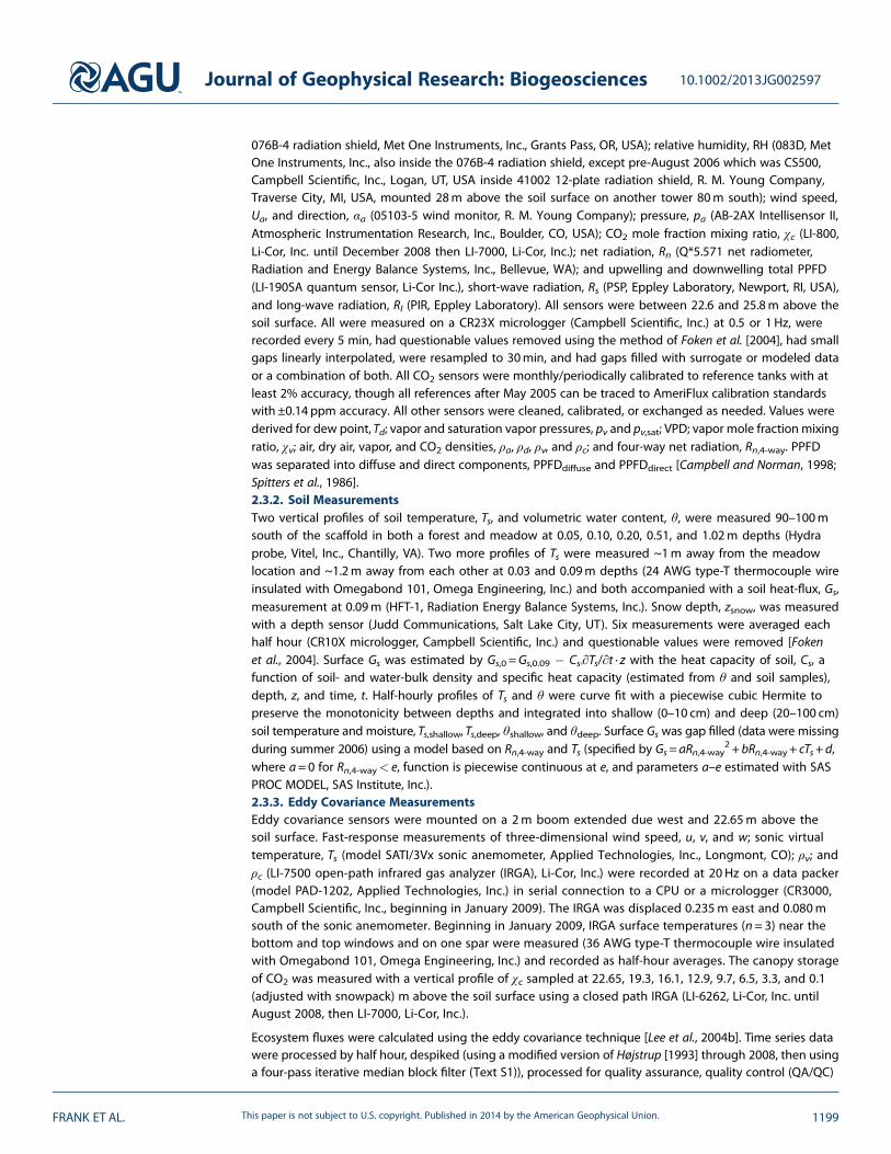
where Y is the response data, the predictor t is time, t50 is the time when half the transition in Y occurs, y50and m are the value and slope of Y at the midpoint, and Δy is the absolute change in Y from midpoint toasymptote (SAS PROC NLMIXED, SAS Institute, Inc., Cary, NC, USA). Consistent with the values of t50, wedetermined phases when the epidemic was characterized by either attacks or mortality. Using these results(section 3.1), the outbreak became epidemic in 2008 at which point over half of the impacted trees had beenattacked (Figure 1). As a consequence, by 2010, the MODIS LAI declined 50% (Figure 1) and 73% of the sprucetrees that accounted for 91% of the spruce basal area were impacted by the beetle (Speckman et al.,manuscript in preparation, 2014). We classified the years 2005–2007 as endemic (characterized by somebackground beetle-caused tree mortality; Figure 2a), 2008–2009 as epidemic I (immediately after the peakbeetle outbreak when impacted trees experience hydraulic failure; Figures 2b and 2c), and 2010 as epidemicII (impacted trees ultimately drop their green needles and die [Mast and Veblen, 1994]; Figure 2d).

2000Date

100

80

60

40

20

0

Tre

es a

ttack

ed b

y be

etle

s (%

)

2002 2004 2006 2008 2010 2012 20140

1

2

3

4

5

6

7

Figure 1. Temporal dynamics of when trees were attacked by beetles relative to when they died. Attacks were determinedfrom our dendrochronological survey. Observable mortality was determined from MODIS LAI. A logistic sigmoid function(equation (1)) was fit to both data sets and estimated that the midpoint of attacks occurred in March 2008 correspondingto the transition from endemic to epidemic I. The midpoint in mortality occurred in January 2010 corresponding to thetransition between epidemic I and II. The estimated difference in transition time between attacks and mortality is1.8 ± 0.9 years, which is consistent with Mast and Veblen [1994] who found that tree ring production in Engelmann sprucestops 1 to 3 years before actual tree death.



https://lpdaac.usgs.gov/data_access

2.2. Tree Physiology Measurements

To quantify the physiological impacts of spruce beetle/blue-stain fungi attack on spruce trees, from 2008 to2010, five healthy and five attacked Engelmann spruce in the vicinity of the AmeriFlux scaffold were sampledwith constant heat sap flux sensors using the methodology of Pataki et al. [2000] and Adelman et al. [2008]which includes local sapwood allometrics to scale themeasurement to the whole tree. Data were fit to a simpleplant hydraulic model [Oren et al., 1999] to relatem, the canopy conductance response to vapor pressure deficit(VPD), to gs,ref, the canopy conductance at a reference VPD of 1.0 kPa, and to test for differences betweenhealthy and attacked trees (SAS PROC GLIMMIX, SAS Institute, Inc.). Calculation of m and gs,ref followed Ewerset al. [2005]. In June, July, and August 2010, five healthy and five attacked trees in the vicinity of the scaffoldwere randomly selected and branches of from the upper third of the crown were collected using a shotgun.Samples were immediately rehydrated so that the measurements reflect photosynthetic capacity. Leaf CO2

assimilation (A) and photosynthetic photon flux density (PPFD) weremeasured for each sample with an LI-6400(Li-Cor, Inc., Lincoln, NE, USA) using the methodology of Long and Bernacchi [2003]. We used a logistic sigmoid(equation (1), with PPFD substituted for t and t50= 0) to test for differences in light response curve parametersbetween healthy and attacked trees (SAS PROC NLMIXED, SAS Institute, Inc.).

2.3. GLEES AmeriFlux Data

All ecosystem flux measurements were made at GLEES AmeriFlux scaffold which was instrumented inOctober 2004. For summer daytime flux data, the 90% effective fetch of scaffold footprint extends0.77 ± 0.18 kmwest at 266 ± 58° (mean± standard deviation) [Gash, 1986] which roughly overlaps the easternhalf of the grid established for our dendrochronological survey (Figure S1) as well as the forest survey plotsused by Speckman et al. (manuscript in preparation, 2014) to determine stand structure and the extent ofbeetle attacks and tree mortality. The scaffold is located in an area that is relatively flat for the region; alongthe average fetch, the slope runs ~4% downhill over 0.5 km to a streambed before rising upward at an ~6%grade. Though advective flows are possible with this topography [Finnigan, 2008], the unusually highturbulence at this site (average u*=1m/s) is the greatest within the AmeriFlux network (http://ameriflux.ornl.gov/) and reduces flux uncertainty due to advection.2.3.1. Meteorological MeasurementsAmbient meteorological measurements were made of air temperature, Ta (RTD-810 resistance thermometerwith OM5-1P4-N100-C signal conditioning module, Omega Engineering, Inc., Stamford, CT, USA, inside

Figure 2. Repeat photography from the GLEES AmeriFlux scaffold showing the three phases of the spruce beetle outbreak:(a) endemic, (b and c) epidemic I, and (d) epidemic II.





076B-4 radiation shield, Met One Instruments, Inc., Grants Pass, OR, USA); relative humidity, RH (083D, MetOne Instruments, Inc., also inside the 076B-4 radiation shield, except pre-August 2006 which was CS500,Campbell Scientific, Inc., Logan, UT, USA inside 41002 12-plate radiation shield, R. M. Young Company,Traverse City, MI, USA, mounted 28m above the soil surface on another tower 80m south); wind speed,Ua, and direction, αa (05103-5 wind monitor, R. M. Young Company); pressure, pa (AB-2AX Intellisensor II,Atmospheric Instrumentation Research, Inc., Boulder, CO, USA); CO2 mole fraction mixing ratio, χc (LI-800,Li-Cor, Inc. until December 2008 then LI-7000, Li-Cor, Inc.); net radiation, Rn (Q*5.571 net radiometer,Radiation and Energy Balance Systems, Inc., Bellevue, WA); and upwelling and downwelling total PPFD(LI-190SA quantum sensor, Li-Cor Inc.), short-wave radiation, Rs (PSP, Eppley Laboratory, Newport, RI, USA),and long-wave radiation, Rl (PIR, Eppley Laboratory). All sensors were between 22.6 and 25.8m above thesoil surface. All were measured on a CR23X micrologger (Campbell Scientific, Inc.) at 0.5 or 1Hz, wererecorded every 5 min, had questionable values removed using the method of Foken et al. [2004], had smallgaps linearly interpolated, were resampled to 30min, and had gaps filled with surrogate or modeled dataor a combination of both. All CO2 sensors were monthly/periodically calibrated to reference tanks with atleast 2% accuracy, though all references after May 2005 can be traced to AmeriFlux calibration standardswith ±0.14 ppm accuracy. All other sensors were cleaned, calibrated, or exchanged as needed. Values werederived for dew point, Td; vapor and saturation vapor pressures, pv and pv,sat; VPD; vapor mole fraction mixingratio, χv; air, dry air, vapor, and CO2 densities, ρa, ρd, ρv, and ρc; and four-way net radiation, Rn,4-way. PPFDwas separated into diffuse and direct components, PPFDdiffuse and PPFDdirect [Campbell and Norman, 1998;Spitters et al., 1986].2.3.2. Soil MeasurementsTwo vertical profiles of soil temperature, Ts, and volumetric water content, θ, were measured 90–100msouth of the scaffold in both a forest and meadow at 0.05, 0.10, 0.20, 0.51, and 1.02m depths (Hydraprobe, Vitel, Inc., Chantilly, VA). Two more profiles of Ts were measured ~1m away from the meadowlocation and ~1.2m away from each other at 0.03 and 0.09m depths (24 AWG type-T thermocouple wireinsulated with Omegabond 101, Omega Engineering, Inc.) and both accompanied with a soil heat-flux, Gs,measurement at 0.09m (HFT-1, Radiation Energy Balance Systems, Inc.). Snow depth, zsnow, was measuredwith a depth sensor (Judd Communications, Salt Lake City, UT). Six measurements were averaged eachhalf hour (CR10X micrologger, Campbell Scientific, Inc.) and questionable values were removed [Fokenet al., 2004]. Surface Gs was estimated by Gs,0 =Gs,0.09 � Cs·∂Ts/∂t · z with the heat capacity of soil, Cs, afunction of soil- and water-bulk density and specific heat capacity (estimated from θ and soil samples),depth, z, and time, t. Half-hourly profiles of Ts and θ were curve fit with a piecewise cubic Hermite topreserve the monotonicity between depths and integrated into shallow (0–10 cm) and deep (20–100 cm)soil temperature and moisture, Ts,shallow, Ts,deep, θshallow, and θdeep. Surface Gs was gap filled (data were missingduring summer 2006) using a model based on Rn,4-way and Ts (specified by Gs= aRn,4-way

2 + bRn,4-way + cTs+ d,where a=0 for Rn,4-way< e, function is piecewise continuous at e, and parameters a–e estimated with SASPROC MODEL, SAS Institute, Inc.).2.3.3. Eddy Covariance MeasurementsEddy covariance sensors were mounted on a 2m boom extended due west and 22.65m above thesoil surface. Fast-response measurements of three-dimensional wind speed, u, v, and w; sonic virtualtemperature, Ts (model SATI/3Vx sonic anemometer, Applied Technologies, Inc., Longmont, CO); ρv; andρc (LI-7500 open-path infrared gas analyzer (IRGA), Li-Cor, Inc.) were recorded at 20 Hz on a data packer(model PAD-1202, Applied Technologies, Inc.) in serial connection to a CPU or a micrologger (CR3000,Campbell Scientific, Inc., beginning in January 2009). The IRGA was displaced 0.235m east and 0.080msouth of the sonic anemometer. Beginning in January 2009, IRGA surface temperatures (n= 3) near thebottom and top windows and on one spar were measured (36 AWG type-T thermocouple wire insulatedwith Omegabond 101, Omega Engineering, Inc.) and recorded as half-hour averages. The canopy storageof CO2 was measured with a vertical profile of χc sampled at 22.65, 19.3, 16.1, 12.9, 9.7, 6.5, 3.3, and 0.1(adjusted with snowpack) m above the soil surface using a closed path IRGA (LI-6262, Li-Cor, Inc. untilAugust 2008, then LI-7000, Li-Cor, Inc.).

Ecosystem fluxes were calculated using the eddy covariance technique [Lee et al., 2004b]. Time series datawere processed by half hour, despiked (using a modified version of Højstrup [1993] through 2008, then usinga four-pass iterative median block filter (Text S1)), processed for quality assurance, quality control (QA/QC)



based on summary statistics (mean, standard deviation, skewness, kurtosis, and missing data [Vickers andMahrt, 1997]), and IRGA calibration adjusted (for ρc based on periodic in situ reference gas calibrations,for ρv based on regression with the ambient meteorological ρv measurement [Meek et al., 1998](SAS PROC AUTOREG, SAS Institute, Inc.) and similar to Loescher et al. [2009] except on a longer time scalecorresponding to weeks or months rather than half hours). Covariances among u, v, and w and with Ts, ρv,and ρc were calculated every half hour from the time series data, rotated into the long-term planar fitcoordinate [Lee et al., 2004a], and time-lag adjusted with the IRGA (half-hour time lags long-term modeledfrom wind speed and direction [Horst and Lenschow, 2009] with an offset optimized to maximize theabsolute covariance within±1 s lag). The covariances between w and u, Ts, ρv, and ρc were spectrally corrected(half-hour corrections [Massman, 2000; Massman and Clement, 2004] based on long-term modeled peakfrequency [Horst, 1997] determined from median-pooled normalized cospectra). Sensible heat (H), watervapor (Fv), and CO2 (Fc) ecosystem fluxes were calculated from the vertical wind covariances using the Webb-Pearman-Leuning (WPL) corrections [Gu et al., 2012; Massman and Lee, 2002; Webb et al., 1980] includingthe additional IRGA self-heating term [Burba et al., 2008] (IRGA surface temperatures measured beginning in

2009, for preceding years modeled based on the 2009 measurements). The canopy storage of CO2, S [Lee andMassman, 2011; W. J. Massman, unpublished derivation, 2010], was calculated using the piecewise cubicHermite interpolated vertical profile of CO2 measured within the canopy. The net ecosystem exchange of

CO2, NEE, was defined as Fc + S [Lee and Massman, 2011]. Evapotranspiration, ET, was defined as Fv and fromwhich latent energy was derived. Atmospheric stability, z/L, and friction velocity, u*, were derived from theeddy covariance data.2.3.4. Canopy ConductanceCanopy conductance to CO2 was calculated from the Penman-Monteith equation [Monteith andUnsworth, 2008] with aerodynamic and boundary layer resistance defined by Massman et al. [1994]. Potentialevapotranspiration (PET) was calculated from the Penman-Monteith equation assuming infinite gc[Penman, 1948].

2.4. Analysis

All analyses were conducted on daytime growing season data. We defined growing season as July–September,which corresponded closely (±8 days) to the intersection among all years of days without snow, standing water,or saturated shallow soil, with a strong daily NEE cycle, and before the magnitude of NEE rapidly decreases inthe fall. Daytime was defined when PPFD> 10μmolm�2 s�1. Data corresponding to u*< 0.2m s�1 (thresholddetermined using the method of Gu et al. [2005]) were not included. To limit outliers, gc outside the range0–300mmolm�2 s�1, PET outside the range�10 to 60mmolm�2 s�1, or gap-filled PPFDwere not included. Noflux data were gap filled. Daily average ET and NEE fluxes were determined by averaging across all non-missingday and night flux measurements with u*≥ 0.2m s�1 occurring at the same half hour of the day across theentire growing season.

We quantified the beetle epidemic impact on the ecosystem by testing for changes in the parametersdescribing the relationships between gc, ET, PET, and NEE and each relative to their primary environmentaldrivers over time and by beetle phase. First, we used analysis of variance (ANOVA) to test for changes in gc.Then, we tested ET relative to PET using a linear model with slope βPET to detect mechanistic changes ingc and ET [Granier, 1987]. This regression required correction for heteroscedasticity of errors (weight= PET�0.7,determined a posteriori). With a change in conductance established, we determined the environmentaldrivers of gc using linear model selection from a pool of candidate variables related to stomatalconductance: PPFD, Ta, VPD, θshallow, θdeep, χc, Ts,shallow, and Ts,deep [Delucia, 1986; Jarvis, 1976; Massmanand Kaufmann, 1991] where soil was separated into shallow (0–10 cm) and deep (20–100 cm) root zonesand θ was a surrogate for leaf water potential assuming the possibility of anisohydric regulation, i.e., leafwater potential is not tightly controlled with increasing water stress, in spruce [Ewers et al., 2005]. Wethen determined the environmental drivers of ET through linear model selection using candidate driversfrom the Penman-Monteith equation: Rn,4-way�Gs (diabatic term); VPD (adiabatic term); Ta, pa, ρa, andρv (variously related to the saturation vapor pressure, latent heat of vaporization, and psychrometricconstant); Ua, u*, and z/L (related to aerodynamic resistance), plus the identified drivers of gc. BecausePenman-Monteith is a semimechanistic model, only the relationships with gc drivers were allowed tovary over time.



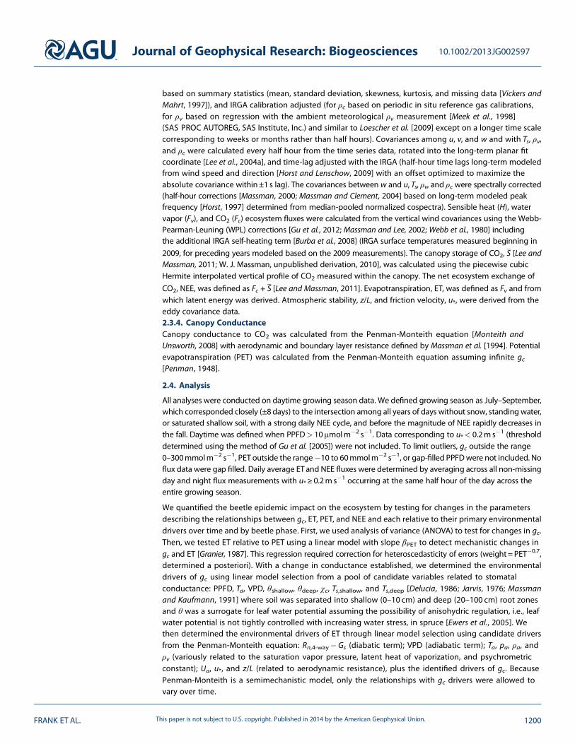
To qualitatively describe relationship betweenNEE and gc, for each year, we fit a locallyweighted regression (LOESS) curve [Cleveland,1979; Cleveland and Devlin, 1988] which is asimple and flexible curve-fitting algorithm thatgives a confidence limit on the predicted fit.We fit and compared the seven saturatingresponse curves proposed by Moffat [2010] tohave functional or historical (i.e., comparableto literature) significance for explaining thesemiempirical NEE response to light (thoughwe analogously extended these to a NEEresponse to gc) plus a linear function andfocused on the logistic sigmoid function(equation (2)) with βgc (initial slope of the NEEversus gc relationship) and Amax (maximum CO2

assimilation rate).

NEE ¼ �Amax tanhβgcgcAmax

� �þ Intercept (2)

To relate NEE to its environmental drivers, wefit three light response curves: a rectangularhyperbola (Michaelis-Menten, equation (3)), alogistic sigmoid [Moffat, 2010] (equation (4)),and a combination of diffuse and directradiation (equation (5)) with Amax (maximumCO2 assimilation rate), Φ, Φdirect, and Φdiffuse

(quantum yields of photosynthesis for total,direct, and diffuse light), and Rd (day respiration).Each equation controlled for VPD [Jarvis, 1976]with a constant βVPD (slope of the vapordeficit relationship):

NEE ¼ � AmaxΦPPFDAmax þ ΦPPFD

1� βVPDVPDð Þ þ Rd (3)

NEE ¼ �Amax tanhΦPPFDAmax

� �1� βVPDVPDð Þ þ Rd (4)

NEE ¼ � ΦdirectPPFDdirect þ ΦdiffusePPFDdiffuseð Þ 1� βVPDVPDð Þ þ Rd (5)

Model selectionwas limited to variables improving overall R2 by at least 0.05 (SAS PROCGLMSELECT, SAS Institute,Inc.). All analyses were done while testing and correcting for autocorrelation of errors (SAS PROC MODEL, SASInstitute, Inc., one time lag) [Bender and Heinemann, 1995; Meek et al., 1998]. Parameters were compared by yearand by epidemic phase, except βVPD which was held constant. All comparisons were Bonferroni corrected formultiple comparisons [Hochberg and Tamhane, 1987]. We checked the sensitivity of all analyses to the Penman-Monteith calculation using other definitions of aerodynamic resistance [Brutsaert, 1982; Campbell and Norman,1998; Monteith and Unsworth, 2008; Thom and Oliver, 1977] as well as the definition of the growing season.

We conducted a meta-analysis of our results to reconcile changes in parameters that most represent thediminishment in ET and NEE, while relating these changes to ecosystem structure and loss of overstoryflux. Declines during epidemic I were not used to determine changes in ecosystem structure because theinterpretation of these years depends on selection of hypothesis a or b. Simultaneously, we tested the sensitivity

g s,ref (mmol m−2 s−1)

m (

mm

ol m

−2

s−1

kPa−

1 )

0 10 20 30 40 50 60 700

5

10

15

20

25

30

35

healthyattacked

(a)

A (

µmol

m−

2 s−

1 )

0 500 1000 1500 2000 2500−3

−2

−1

0

1

2

3

4

PPFD (µmol m−2 s−1)

(b)

Figure 3. Tree physiological impacts of spruce beetle/blue-stain fungus on Engelmann spruce. (a) Sap flux data fromhealthy and attacked trees fit a simple hydraulic model [Orenet al., 1999] relating the slope of the canopy conductanceresponse to vapor pressure deficit VPD (m) to canopy conduc-tance at a reference VPD of 1.0 kPa (gs,ref). The region 0.5–0.6(dashed lines) represents most plant taxa [Katul et al., 2009]. (b)Photosynthetic assimilation (A) response to photosyntheticphoton flux density (PPFD) from hydrated branches sampledfrom healthy and attacked trees fit to the logistic sigmoidfunction (equation (1)). Data are jittered 2% of full scale inFigure 3b for display purposes.



of βPET to the formulation of boundary layerresistance [Brutsaert, 1982; Kaimal and Finnigan,1994; Massman et al., 1994; Monteith andUnsworth, 2008; Thom and Oliver, 1977]. This wasdone using a hierarchical Bayesian random-effects model [Gelman et al., 2004; Rubin, 1981].The modeled data were the mean and standarderrors of the regression parameters Φ, Amax,Φdirect, Φdiffuse, and βPET. Gamma distributionswere used as priors for parameters representingthe distributions of the regression parametersduring the endemic phase. Priors for thehyperparameters were either flat distributions(pre-epidemic contribution of transpiration, T,to ET and overstory to total ecosystem flux)or gamma distributions (the relative changesin overstory, NEE, and ET from the endemicto epidemic I or II phases; random effects inthe changes in NEE and ET due to choice ofboundary layer resistance or light responseparameter). Analysis was conducted withOpenBUGS (version 3.2.2 rev 1063, Members ofOpenBUGS Project Management Group). Thesource code is provided in Text S2.

3. Results3.1. When Trees Were Attacked and When They Died

We successfully cored and dated 109 Engelmann spruce and 38 subalpine fir trees, of which 79 wererecently dead including 74 spruce (Figure 1 and Table S1). Spruce were older and larger (268 ± 163 yearsmean± standard deviation, 44 ± 23 cm diameter at breast height) than fir (161 ± 76 years, 27 ± 11 cm) whiledead spruce were older and larger (307 ± 165 years, 53 ± 23 cm) than live spruce (186± 126 years and25± 9 cm) (Table S1). The average age to coring height was 35 ± 17 years. Tree establishment dated to the1200s while the age structure coincided with climatic events and not disturbances (Text S3).

The number of attacks was greatest in 2008 (Figure 1). The regression parameters (estimate ± standard error)for the logistic sigmoid predicting attacks were y50 = 0.30 ± 0.004%, Δy = 0.30 ± 0.007%,m= 0.00037 ± 0.000016%/d, t50 = 3 March 2008± 0.0 day (Figure 1). The reduction in LAI following mortalityoccurred much later (1.8 ± 0.9 years); the regression parameters for LAI were y50 = 3.76 ± 0.198m2m�2,Δy= 0.89 ± 0.203m2m�2, m= �0.00107 ± 0.000315m2m�2/d, t50 = 3 January 2010 ± 339 days (Figure 1).

3.2. The Physiology Effect of Beetle Attacks on Spruce Trees

Our sap flux data show that the conductance gs,ref was significantly lower for Engelmann spruce attackedby spruce beetle/blue-stain fungus (p< 0.0001) but that the slope of the relationship m to gs,ref was notdifferent for healthy or attacked trees (p = 0.81) or the 0.5–0.6 region (p> 0.61) described by Katul et al.[2009] (Figure 3a). There also was no difference in photosynthesis between hydrated branches sampledfrom healthy or attacked trees (p> 0.18 for all parameters after fitting the logistic sigmoid function(equation (1)); Figure 3b).

3.3. Precipitation and Soil Moisture

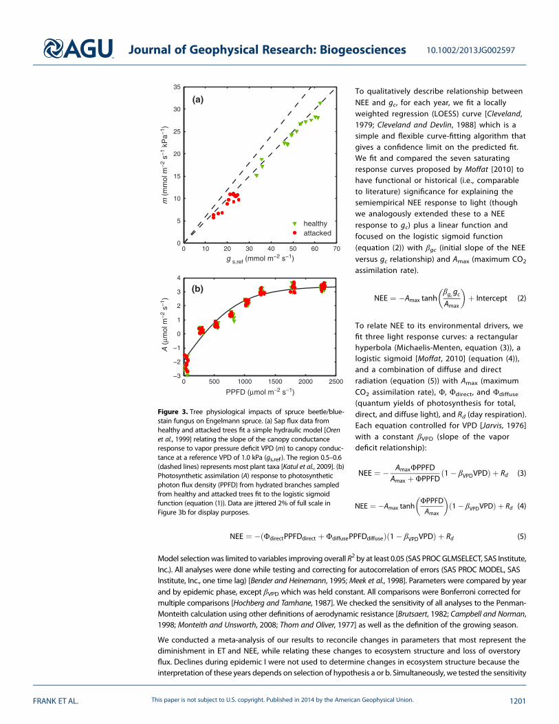
The climate at GLEES is dominated by winter moisture (Figure 4a). More precipitation accumulated fromthe beginning of the water year (1 October) until the end of June during the epidemic years, while theaccumulations in 2005 and 2007 were noticeably deficient by over 200mm (Figure 4a). Summer precipitationat GLEES is much lower, and though 2006 and 2007 were relatively moist, 2005 was 30mm drier than anyother year (Figure 4b). Soil moisture was generally equal or higher during the epidemic years: θshallow was

O N D J F M A M J J A S O0

200

400

600

800

1000

1200

1400

Month of Water Year

Cum

ulat

ive

Pre

cipi

tatio

n (m

m)

J A S O0

50

100

150

200

200520062007200820092010

(a)

(b)

Figure 4. Cumulative precipitation at GLEES during (a) the wateryear (1 October to 30 September) and (b) the summer growingseason (July–September) for the endemic (2005–2007) andepidemic (2008–2010) years. Data from the National AtmosphericDeposition Program WY95 site (http://nadp.sws.uiuc.edu/) 200mfrom the AmeriFlux scaffold.



http://nadp.sws.uiuc.edu/

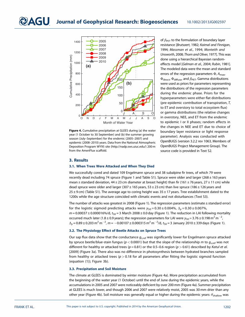
higher in July before becoming more similar toendemic levels duringmiddle and late summer(Figure 5a) and θdeep was higher throughoutthe entire season (Figure 5b).

3.4. Average Daily Ecosystem Fluxes

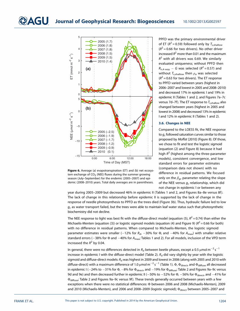
The average daily ET fluxes appeared higherduring the endemic years (Figure 6a) andwhenextrapolated over the entire growing seasonranged from 245 to 260mm during 2005–2007and 204 to 218mm during the epidemic years2008–2010. The average daily NEE fluxesappeared to decrease in magnitude duringepidemic I and then further in epidemic II(Figure 6b). When extrapolated over thegrowing season, the ecosystem carbon sinkranged from163 to 234gCm�2 for the endemicyears, 83 to 112 g C m�2 for epidemic I, and�5 g C m�2 for epidemic II.

Yet these observations are difficult to testand support statistically; thus, we focus ouranalysis on response curves of half hourlyfluxes in the following sections. For these, allparameter comparisons were significant(p< 0.05) unless otherwise noted. All analysesincluded an autoregressive model (Durbin-Watson statistic increased from 0.55–1.26 to1.98–2.27) that typically increased the relativestandard errors of parameters but, in somecircumstances, altered the parameter estimates(�7% forΦ,�10% forAmax,�17% for Rd,�19%

forΦdirect, +22% forΦdiffuse, and�65% for βgc). The Breusch-Pagan test for heteroscedasticity of errors in the ETversus PET relationship was significant (p< 0.0001) before controlling with a weighted regression (p=0.08).

3.5. Changes in Canopy Conductance and Evapotranspiration

During the spruce beetle epidemic, average gc decreased 17% while ET decreased 22% relative to PET(Tables 1 and 2, and Figures S2a–S2c versus S2d–S2f ). There were no differences in gc between any ofthe endemic years (2005–2007) nor were there differences between any of the epidemic years (phases Iand II, 2008–2010) except for some minor intercept differences (<0.2mmolm�2 s�1) in the ET versusPET relationship (Tables 1 and 2). The ET/PET analyses were sensitive to the definition of aerodynamicresistance; there were significant differences between epidemic I and II and greater parameter decreases(Tables S2 and S3).

Through model selection, PPFD was identified as the primary environmental driver of gc (R2 = 0.21), followed

by VPD (R2 = 0.39 for two drivers), and Ts,shallow (R2 = 0.47 for three drivers). No other driver (Ta, Ts,deep, θshallow,θdeep, or χc) increased R2 by more than 0.01 and the maximum R2 with all drivers was 0.50. Model selectionwas also performed without each driver to determine its uniqueness: Without PPFD then VPD was selected(R2 = 0.10), without VPD then Ta was selected (R2 = 0.28 for two drivers), and without Ts,shallow then Ta wasselected (R2 = 0.44 for three drivers). The gc response to PPFD did change between years (highest in 2007 andlowest in 2008 and 2009) and it significantly decreased 14% in epidemic I while the 9% decrease in epidemicII was not significant (Tables 1 and 2). The gc response to VPD did not change over time. Tree hydraulicanalysis of sap flux data supported hydraulic failure as the mechanism for gc decline (Figure 3a). The gcresponse to Ts,shallow also changed between years (highest in 2005, lowest in 2007–2010) which equaled a20% decrease during epidemic I and a 24% in epidemic II (Tables 1 and 2).

Figure 5. Range of daily (a) shallow and (b) deep soil moisture (θ)during the summer growing season (July–September) for theendemic (2005–2007) and epidemic (2008–2010) years.



PPFD was the primary environmental driverof ET (R2 = 0.59) followed only by Ts,shallow(R2 = 0.66 for two drivers). No other driverincreased R2 more than 0.01 and themaximumR2 with all drivers was 0.69. We similarlyevaluated uniqueness; without PPFD thenRn,4-way � G was selected (R2 = 0.57) andwithout Ts,shallow then ρa was selected(R2 = 0.63 for two drivers). The ET responseto PPFD varied between years (highest in2006–2007 and lowest in 2005 and 2008–2010)and decreased 17% in epidemic I and 19% inepidemic II (Tables 1 and 2, and Figures 7a–7cversus 7d–7f). The ET response to Ts,shallow alsochanged between years (highest in 2005 andlowest in 2008) and decreased 13% in epidemicI and 12% in epidemic II (Tables 1 and 2).

3.6. Changes in NEE

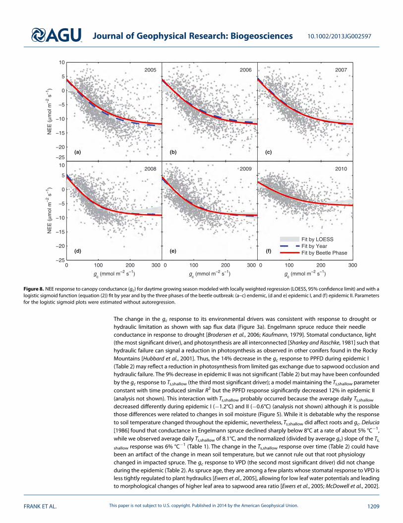
Compared to the LOESS fit, the NEE responseto gc followed saturation curves similar to thoseproposed by Moffat [2010] (Figure 8). Of those,we chose to fit and test the logistic sigmoid(equation (2) and Figure 8) because it hadhigh R2 (highest among the three-parametermodels), consistent convergence, and lowstandard errors for parameter estimates(comparison data not shown) with nodifference in residual patterns. We focusedonly on the βgc parameter relating the slopeof the NEE versus gc relationship, which didnot change in epidemic I or between any

year during 2005–2009 but decreased 46% in epidemic II (Tables 1 and 2, and Figures 8a–8e versus 8f ).The lack of change in this relationship before epidemic II is supported by the lack of change in theresponse of needle photosynthesis to PPFD as the trees died (Figure 3b). Thus, hydraulic failure led to lowgc as water transport failed, but the trees were able to maintain leaf water status such that photosyntheticbiochemistry did not decline.

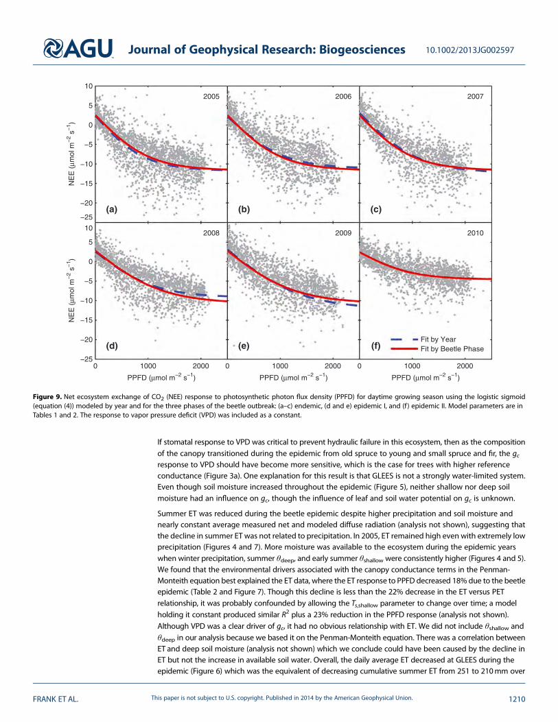
The NEE response to light was best fit with the diffuse-direct model (equation (5), R2 = 0.74) than either theMichaelis-Menten (equation (3)) or logistic sigmoid models (equation (4) and Figure 9) (R2 = 0.66 for both)with no difference in residual patterns. When compared to Michaelis-Menten, the logistic sigmoidparameter estimates were smaller (�12% for Rd, �30% for Φ, and �40% for Amax) with smaller relativestandard errors (�38% for Φ and �40% for Amax; Tables 1 and 2). For all models, inclusion of the VPD termincreased the R2 by 0.04.

In general, there were no differences detected in Rd between beetle phases, except a 0.5μmolm�2 s�1

increase in epidemic I with the diffuse-direct model (Table 2). Rd did vary slightly by year with the logisticsigmoid and diffuse-direct models: Rdwas highest in 2009 and lowest in 2006 (along with 2005 and 2010 withdiffuse-direct) with a maximum difference of 1.0μmolm�2 s�1 (Table 1). Φ, Φdirect, and Φdiffuse all decreasedin epidemic I (�24% to �31% for Φ, �8% for Φdirect, and �19% for Φdiffuse; Table 2 and Figures 9a–9c versus9d and 9e) and then decreased further in epidemic II (�50% to �52% for Φ, �56% for Φdirect, and �41% forΦdiffuse; Table 2 and Figures 9a–9c versus 9f). These trends generally occurred between years with a fewexceptions when there were no statistical differences: Φ between 2006 and 2008 (Michaelis-Menten), 2009and 2010 (Michaelis-Menten), and 2006 and 2008–2009 (logistic sigmoid); Φdirect between 2005–2007 and

0

1

2

3

4

5

ET

(m

mol

m−

2 s−

1 )

2005 (1.7)2006 (1.8)2007 (1.8)2008 (1.5)2009 (1.5)2010 (1.4)

0:00 6:00 12:00 18:00−15

−10

−5

0

5

Time of Day (MST)

NE

E (

µmol

m−

2 s−

1 )

2005 (−2.5)2006 (−1.9)2007 (−1.7)2008 (−1.2)2009 (−0.9)2010 (0.1)

(b)

(a)

Figure 6. Average (a) evapotranspiration (ET) and (b) net ecosys-tem exchange of CO2 (NEE) fluxes during the summer growingseason (July–September) for the endemic (2005–2007) and epi-demic (2008–2010) years. Total daily averages are in parentheses.



2009; and Φdiffuse between 2006 and 2009 (Table 1). Amax did not change until epidemic II when it decreased51% (Table 2 and Figures 9a–9e versus 9f ). There was some variation from 2005 to 2009: Amax was highest in2009 (plus 2007 with the logistic sigmoid) and lowest in 2008.

3.7. Meta-analysis

Posterior densities for the decreases in ET and NEE were approximately normally distributed. ET changed by�28± 4% and�36± 4% during epidemic I and II (the 95% credible intervals overlapped), while NEE changedby�13± 6% and�51± 3% similarly (mean± standard deviation; Table S4). The pre-epidemic contribution ofoverstory to total ecosystem flux as well as the loss of overstory flux was >50% (Figures S3a and S3b, andTable S4) and highly correlated (Figure S3d). While the contribution of T to ET had a large range (95% credibleinterval from 55 to 89%; Table S4), the posterior density was more defined with an obvious peak at 71%(Figure S3c).

4. Discussion

We observed through cessation of tree ring growth [Mast and Veblen, 1994] that even though beetleattacks occurred throughout the past decade, 2008 was the year both of peak attack and when thenumber of impacted trees crossed the 50% threshold (Figure 1). But, as observed in the MODIS LAIdata (Figure 1) and our repeat photos (Figure 2), observable tree mortality had a different temporalpattern from attacks, and did not occur until 1.8 ± 0.9 years later. This supports our definition of threephases (endemic, epidemic I, and epidemic II), is consistent with previous observations in Engelmann

Table 1. Summary of All Statistical Tests With Respect to Year

Year

Comparison Function Regression Parameters 2005 2006 2007

gc ANOVA gc (mmolm�2 s�1) 115.9 (2.27)b 124.2 (2.47)b 116.6 (2.65)b

φ �0.668 (0.0085)*

ET versus PET Linear Intercept (mmolm�2 s�1) 0.476 (0.0351)a,b 0.517 (0.0356)b 0.529 (0.0423)b

βPET (mmolmmol�1) 0.0907 (0.00204)b 0.0994 (0.00215)b 0.0976 (0.00245)b

φ �0.594 (0.0087)*

gc versusenvironmental drivers

Linear Intercept (mmolm�2 s�1) 81.9 (2.14)*

βPPFD (mmolμmol�1) 0.0519 (0.00210)a,b 0.0603 (0.00229)b,c 0.0619 (0.00257)c

βVPD (mmolm�2 s�1 kPa�1) �102.5 (4.22)a �89.3 (4.56)a �89.4 (4.94)a

βTs,shallow (mmolm�2 s�1 C�1) 8.80 (0.472)b 7.30 (0.461)a,b 6.53 (0.516)a

φ �0.403 (0.0101)*

ET versusenvironmental drivers

Linear Intercept (mmolm�2 s�1) �0.58 (0.049)*

βPPFD (mmolμmol�1) 0.00187 (0.000046)a 0.00214 (0.000048)b 0.00231 (0.000053)b

βTs,shallow (mmolm�2 s�1 C�1) 0.162 (0.0073)c 0.157 (0.0070)b,c 0.134 (0.0076)a,b

φ �0.478 (0.0087)*

NEE versus gc Logistic sigmoid(equation (1))

Intercept (μmolm�2 s�1) 0.2 (0.30)a 0.9 (0.31)a,b 1.0 (0.32)a,b

βgc,C (μmolmmol�1) 0.0463 (0.00400)b 0.0392 (0.00350)b 0.0427 (0.00344)b

Amax (μmolm�2 s�1) 9.3 (0.52)a,b 10.0 (0.82)b 13.3 (1.73)b

φ �0.893 (0.0057)*

NEE versusenvironmental drivers

Rectangular hyperbola(Michaelis-Menten,

equation (2))

Rd (μmolm�2 s�1) 2.8 (0.21)a 2.6 (0.22)a 3.4 (0.24)a

Φ (molmol�1) 0.0281 (0.00156)d 0.0225 (0.00143)c,d 0.0242 (0.00147)d

Amax (μmolm�2 s�1) 27.1 (0.98)b,c 26.8 (1.19)b,c 31.3 (1.49)c,d

βVPD (kPa�1) 0.202 (0.0098)*

φ �0.773 (0.0065)*

Logistic sigmoid(equation (3))

Rd (μmolm�2 s�1) 2.4 (0.19)a,b 2.2 (0.20)a 3.0 (0.21)a,b

Φ (molmol�1) 0.0183 (0.00064)d 0.0153 (0.00060)b,c 0.0165 (0.00062)d,c

Amax (μmolm�2 s�1) 17.3 (0.43)c,d 16.4 (0.45)c 18.7 (0.55)d

βVPD (kPa�1) 0.200 (0.0102)*

φ �0.775 (0.0065)*

Linear (equation (4)) Rd (μmolm�2 s�1) 2.6 (0.17)a 2.6 (0.18)a 3.3 (0.20)a,b

Φdirect (molmol�1) 0.0076 (0.00020)c 0.0072 (0.00020)c 0.0084 (0.00023)d

Φdiffuse (molmol�1) 0.0205 (0.00050)e 0.0176 (0.00049)c,d 0.0192 (0.00054)d,e

βVPD (kPa�1) 0.223 (0.0080)*

φ �0.712 (0.0072)*



spruce of a 1 to 3 year delay between attack and mortality [Mast and Veblen, 1994], is explained by ourtree physiology data that show attacked trees still maintain leaf biochemistry, and supports hypothesis band its predictions.

The first-order effects of a beetle epidemic occur at the plant scale. Blue-stain fungi impacts on the hydraulicsof Engelmann spruce fit the expectations of a simple plant hydraulic model [Oren et al., 1999] (Figure 3a).Because the slopes of healthy and attacked trees are not different from each other or the 0.5–0.6 region [Katulet al., 2009] (Figure 3a), this indicates that the trees are regulating minimum leaf water potential as hydraulicconductance declines [Ewers et al., 2005; Oren et al., 1999]. At the same time, the blue-stain fungi do notimpact leaf photosynthetic biochemistry (Figure 3b) but hydraulic limitation leads to decreased C uptakefrom gas exchange limitations while trees are dying from attacks. These data strongly support the hypothesisthat trees are dying from hydraulic failure by fungal xylem occlusion but maintain leaf biochemistry byreducing stomatal conductance to prevent excessive dehydration of foliage.

To evaluate our two competing hypothesis that (a) changes in ecosystem fluxes can be inferred simplyfrom the observable patterns of mortality or (b) that physiological impacts in the attacked trees must alsobe incorporated, we must understand how the responses of gc, ET, and NEE to their environmental drivers

Table 1. (continued)

Year Without Correcting for Autocorrelation of Errors Correcting for Autocorrelation of Errors

2008 2009 2010 N R2 RMSE DW R2 RMSE DW

96.5 (2.43)a 96.4 (2.47)a 101.1 (2.37)a 10398 0.039 55.7 0.70 0.397 44.1 2.07

0.482 (0.0382)a,b 0.362 (0.0374)a 0.393 (0.0419)a,b 10142 0.518 1.06 0.81 0.756 0.29 2.100.0725 (0.00219)a 0.0795 (0.00237)a 0.0735 (0.00226)a

0.0495 (0.00225)a 0.0494 (0.00221)a 0.0523 (0.00215)a,b,c 10396 0.473 41.3 1.26 0.542 38.5 2.03�89.3 (4.68)a �93.8 (4.42)a �94.8 (4.02)a

6.13 (0.522)a 6.10 (0.503)a 5.84 (0.464)a

0.00180 (0.000048)a 0.00168 (0.000048)a 0.00168 (0.000047)a 11338 0.658 0.97 1.09 0.729 0.86 2.160.129 (0.0078)a 0.136 (0.0079)a,b 0.133 (0.0080)a,b

1.4 (0.29)b 1.2 (0.28)a,b 1.2 (0.27)a,b 10387 0.463 3.7 0.66 0.760 2.4 1.980.0383 (0.00425)b 0.0393 (0.00364)b 0.0227 (0.00312)a

7.0 (0.53)a 8.4 (0.71)a,b 6.5 (1.37)a,b

2.9 (0.22)a 3.4 (0.21)a 2.5 (0.21)a 11327 0.665 3.0 0.56 0.846 2.0 2.250.0178 (0.00133)b,c 0.0170 (0.00104)a,b 0.0120 (0.00144)a

24.6 (1.47)b 35.5 (2.36)d 13.8 (1.13)a

2.6 (0.20)a,b 3.1 (0.19)b 2.4 (0.20)a,b 11327 0.661 3.0 0.55 0.846 2.0 2.250.0127 (0.00060)b 0.0132 (0.00051)b 0.0085 (0.00062)a

14.4 (0.50)b 18.7 (0.64)d 8.5 (0.40)a

2.9 (0.18)a,b 3.6 (0.18)b 2.8 (0.18)a 11327 0.749 2.6 0.78 0.856 2.0 2.270.0063 (0.00021)b 0.0077 (0.00020)c,d 0.0034 (0.00019)a

0.0154 (0.00051)b 0.0156 (0.00048)b,c 0.0112 (0.00050)a

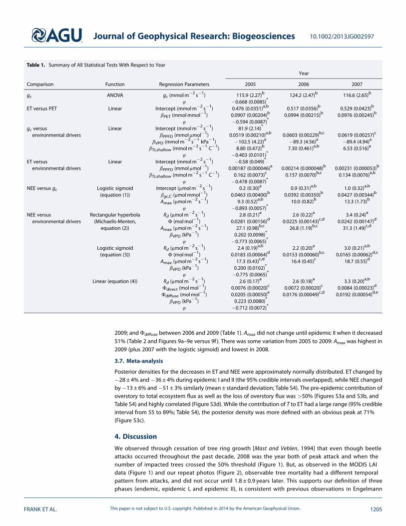
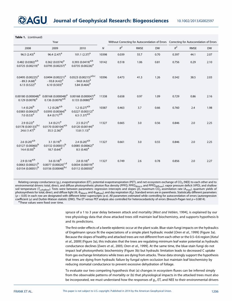
Relating canopy conductance (gc), evapotranspiration (ET), potential evapotranspiration (PET), and net ecosystem exchange of CO2 (NEE) to each other and toenvironmental drivers: total, direct, and diffuse photosynthetic photon flux density (PPFD, PPFDdirect, and PPFDdiffuse), vapor pressure deficit (VPD), and shallowsoil temperature (Ts,shallow). Tests were between parameters: regression intercepts and slopes (β), maximum CO2 assimilation rate (Amax), quantum yields ofphotosynthesis for total, direct, and diffuse light (Φ,Φdirect, andΦdiffuse), and day respiration (Rd). Standard errors are in parenthesis. Statistically different parameters(p< 0.05) in each row are designated with different letter superscripts (a-e). All parameters estimated while controlling for autocorrelation of errors (autoregressioncoefficient (φ) and Durbin-Watson statistic (DW)). The ET versus PET analysis also controlled for heteroscedasticity of errors (Breusch-Pagan test p=0.0814).*These values were fixed over time.



Table

2.Su

mmaryof

AllStatisticalTestsWith

Respectto

BeetlePh

ase

Beetle

Phase

With

outCorrectingfor

Autocorrelatio

nof

Errors

Correctingfor

Autocorrelatio

nof

Errors

Com

parison

Functio

nRe

gression

Parameters

Ende

mic

Epidem

icI

Epidem

icII

NR2

RMSE

DW

R2RM

SEDW

g cANOVA

g c(m

molm�2s�

1)

118.8(1.42)b

96.5(1.74)a

101.2(2.38)a

1039

80.03

655

.80.70

0.39

744

.12.08

φ�0

.670

(0.008

5)*

ETversus

PET

Line

arIntercep

t(m

molm�2s�

1 )0.50

5(0.021

6)a

0.42

3(0.026

8)a

0.39

5(0.042

0)a

1014

20.51

21.06

0.80

0.75

50.29

2.10

β PET

(mmolmmol�1

)0.09

53(0.001

28)b

0.07

56(0.001

62)a

0.07

34(0.002

27)a

φ�0

.598

(0.008

6)*

g cversus

environm

ental

drivers

Line

arIntercep

t(m

molm�2s�

1 )81

.8(2.15)*

1039

60.46

841

.41.25

0.54

038

.52.03

β PPFD

(mmolμm

ol�1 )

0.05

75(0.001

35)b

0.04

94(0.001

59)a

0.05

23(0.002

16)a,b

β VPD(m

molm�2s�

1kPa�

1 )�9

4.4(2.64)a

�91.2(3.24)a

�94.8(4.06)a

β Ts,shallow(m

molm�2s�

1C�1)

7.65

(0.315

)b6.10

(0.388

)a5.85

(0.467

)a

φ�0

.409

(0.010

1)*

ETversus

environm

ental

drivers

Line

arIntercep

t(m

molm�2s�

1 )�0

.58(0.049

)*11

338

0.65

40.97

1.08

0.72

80.86

2.17

β PPFD

(mmolμm

ol�1)

0.00

208(0.000

029)b0.00

174(0.000

035)a0.00

168(0.000

048)a

β Ts,shallow(m

molm�2

s�1C�

1 )0.15

2(0.005

6)b

0.13

2(0.006

6)a

0.13

3(0.008

1)a

φ�0

.483

(0.008

7)*

NEE

versus

g cLogisticsigm

oid

(equ

ation(4))

Intercep

t(μmolm�2

s�1 )

0.6(0.18)a

1.3(0.20)b

1.2(0.27)a,b

1038

70.45

83.7

0.65

0.75

92.5

1.98

β gc,C(μmolmmol�1)

0.04

23(0.002

10)b

0.03

89(0.002

79)b

0.02

27(0.003

13)a

Amax

(μmolm�2s�

1)

10.4(0.48)b

7.6(0.43)a

6.5(1.37)ab

φ�0

.893

(0.005

7)*

NEE

versus

environm

ental

drivers

Rectangu

larhype

rbola

(Michaelis-M

enten,

equatio

n(1)

R d(μmolm�2s�

1)

2.9(0.13)a

3.1(0.15)a

2.5(0.21)a

1132

70.65

93.0

0.54

0.84

52.0

2.25

Φ(m

olmol�1)

0.02

51(0.000

87)c

0.01

72(0.000

82)b

0.01

20(0.001

45)a

Amax

(μmolm�2s�

1)

27.9(0.77)b

29.8(1.40)b

13.8(1.12)a

β VPD(kPa

�1)

0.19

9(0.009

9)*

φ�0

.773

(0.006

5)*

Logisticsigm

oid

(equ

ation(2))

R d(μmolm�2s�

1)

2.5(0.12)a

2.8(0.14)a

2.4(0.20)a

1132

70.65

53.1

0.54

0.84

52.0

2.25

Φ(m

olmol�1)

0.01

67(0.000

38)c

0.01

28(0.000

39)b

0.00

84(0.000

62)a

Amax

(μmolm�2s�

1)

17.3(0.33)b

16.5(0.44)b

8.5(0.40)a

β VPD(kPa

�1)

0.19

7(0.010

3)*

φ�0

.776

(0.006

5)*

Line

ar(equ

ation(3))

R d(μmolm�2s�

1)

2.8(0.11)a

3.3(0.13)b

2.8(0.18)a,b

1132

70.74

02.6

0.75

0.85

52.0

2.28

Φdirect(m

olmol�1

)0.00

76(0.000

14)c

0.00

70(0.000

16)b

0.00

33(0.000

19)a

Φdiffuse

(molmol�1)

0.01

90(0.000

32)c

0.01

54(0.000

36)b

0.01

11(0.000

50)a

β VPD(kPa

�1)

0.21

9(0.008

1)*

φ�0

.718

(0.007

2)*

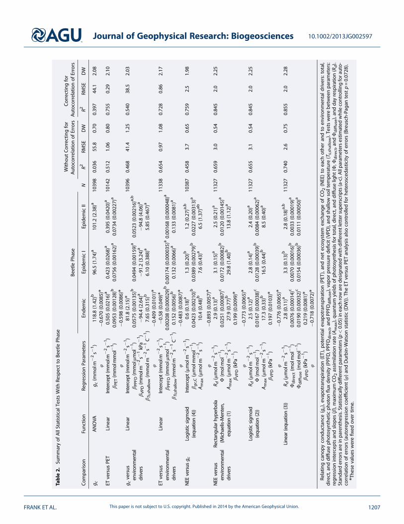
Relatin

gcano

pycond

uctance(gc),e

vapo

tran

spira

tion(ET),p

oten

tiale

vapo

tran

spira

tion(PET

),an

dne

tecosystem

exchan

geof

CO2(NEE)to

each

othe

ran

dto

environm

entald

rivers:total,

direct,and

diffuseph

otosyn

theticph

oton

flux

density

(PPF

D,PPFDdirect,and

PPFD

diffuse),vapo

rpressure

deficit(VPD

),an

dshallowsoiltempe

rature

(Ts,shallow).Testswerebe

tweenpa

rameters:

regression

intercep

tsan

dslop

es(β),maxim

umCO2assimilatio

nrate

(Amax),qu

antum

yields

ofph

otosyn

thesisfortotal,direct,and

diffuselig

ht(Φ

,Φdirect,and

Φdiffuse),an

dda

yrespira

tion(Rd).

Stan

dard

errorsareinpa

renthe

sis.Statisticallydifferen

tparam

eters(p<0.05

)ineach

rowarede

sign

ated

with

differen

tlettersup

erscrip

ts(a-c).Allpa

rametersestim

ated

whilecontrolling

fora

uto-

correlationof

errors(autoreg

ressioncoefficien

t(φ)a

ndDurbin-Watsonstatistic

(DW)).

TheET

versus

PETan

alysisalso

controlledforhe

terosced

asticity

oferrors(Breusch-Pag

antestp=0.07

28).

*The

sevalues

werefixedov

ertim

e.



changed over the course of the beetle outbreak. That is, which explains the data better: (a) gc, ET, and NEE alldiminish in concert with mortality and reduced LAI, or (b) there was an initial phase (epidemic I)corresponding to beetle attacks and dominated by hydraulic failure (reduced gc and ET) and restricted gasexchange (reduced NEE) followed by a second phase (epidemic II) corresponding to mortality (furtherreduced NEE).

4.1. Changes in Canopy Conductance and Evapotranspiration

The bark beetles fundamentally altered the conductance of water vapor from the ecosystem duringthe first phase of the epidemic. There was a 22% decreased in ET relative to PET that occurred beforethe 2008 summer growing season (Tables 1 and 2, and Figure S2). Because the ET versus PETrelationship implicitly accounts for climate through the Penman-Monteith equation, this reductionreflects a mechanistic change in the ecosystem independent of any changes in the environment. Wepropose that xylem occlusion caused by the beetle-associated blue-stain fungi is the cause of thismechanistic change.

Blue-stain fungi play a vital role in bark beetle infestations by helping overcome tree defenses withfungal penetration and sapwood occlusion [Paine et al., 1997] and can do so quickly over a few weeksas observed with mountain pine beetle [Hubbard et al., 2013; Yamaoka et al., 1990]. Leptographiumabietinum is the most common mycelial fungus isolated from spruce beetle [Six and Bentz, 2003]though Ceratocystis rufipenni is often found in infested Engelmann spruce [Wingfield et al., 1997]. C.rufipenni is believed to be more important in helping spruce beetle overcome the tree’s defenses. In anexperiment with Sitka spruce, C. rufipenni was found to be three to nine times more pathogenic[Solheim and Safranyik, 1997].

Figure 7. Evapotranspiration (ET) response to photosynthetic photon flux density (PPFD) for daytime growing season modeled by year and for the three phases ofthe beetle outbreak: (a–c) endemic, (d and e) epidemic I, and (f ) epidemic II. Model parameters are in Tables 1 and 2. The response to average soil temperature(Ts,shallow) was included as a constant.



The change in the gc response to its environmental drivers was consistent with response to drought orhydraulic limitation as shown with sap flux data (Figure 3a). Engelmann spruce reduce their needleconductance in response to drought [Brodersen et al., 2006; Kaufmann, 1979]. Stomatal conductance, light(the most significant driver), and photosynthesis are all interconnected [Sharkey and Raschke, 1981] such thathydraulic failure can signal a reduction in photosynthesis as observed in other conifers found in the RockyMountains [Hubbard et al., 2001]. Thus, the 14% decrease in the gc response to PPFD during epidemic I(Table 2) may reflect a reduction in photosynthesis from limited gas exchange due to sapwood occlusion andhydraulic failure. The 9% decrease in epidemic II was not significant (Table 2) but may have been confoundedby the gc response to Ts,shallow (the third most significant driver); a model maintaining the Ts,shallow parameterconstant with time produced similar R2 but the PPFD response significantly decreased 12% in epidemic II(analysis not shown). This interaction with Ts,shallow probably occurred because the average daily Ts,shallowdecreased differently during epidemic I (�1.2°C) and II (�0.6°C) (analysis not shown) although it is possiblethose differences were related to changes in soil moisture (Figure 5). While it is debatable why the responseto soil temperature changed throughout the epidemic, nevertheless, Ts,shallow did affect roots and gc. Delucia[1986] found that conductance in Engelmann spruce declined sharply below 8°C at a rate of about 5% °C�1,while we observed average daily Ts,shallow of 8.1°C, and the normalized (divided by average gc) slope of the Ts,shallow response was 6% °C�1 (Table 1). The change in the Ts,shallow response over time (Table 2) could havebeen an artifact of the change in mean soil temperature, but we cannot rule out that root physiologychanged in impacted spruce. The gc response to VPD (the second most significant driver) did not changeduring the epidemic (Table 2). As spruce age, they are among a few plants whose stomatal response to VPD isless tightly regulated to plant hydraulics [Ewers et al., 2005], allowing for low leaf water potentials and leadingto morphological changes of higher leaf area to sapwood area ratio [Ewers et al., 2005; McDowell et al., 2002].

Figure 8. NEE response to canopy conductance (gc) for daytime growing seasonmodeled with locally weighted regression (LOESS, 95% confidence limit) and with alogistic sigmoid function (equation (2)) fit by year and by the three phases of the beetle outbreak: (a–c) endemic, (d and e) epidemic I, and (f) epidemic II. Parametersfor the logistic sigmoid plots were estimated without autoregression.



If stomatal response to VPD was critical to prevent hydraulic failure in this ecosystem, then as the compositionof the canopy transitioned during the epidemic from old spruce to young and small spruce and fir, the gcresponse to VPD should have become more sensitive, which is the case for trees with higher referenceconductance (Figure 3a). One explanation for this result is that GLEES is not a strongly water-limited system.Even though soil moisture increased throughout the epidemic (Figure 5), neither shallow nor deep soilmoisture had an influence on gc, though the influence of leaf and soil water potential on gc is unknown.

Summer ET was reduced during the beetle epidemic despite higher precipitation and soil moisture andnearly constant average measured net and modeled diffuse radiation (analysis not shown), suggesting thatthe decline in summer ET was not related to precipitation. In 2005, ET remained high even with extremely lowprecipitation (Figures 4 and 7). More moisture was available to the ecosystem during the epidemic yearswhen winter precipitation, summer θdeep, and early summer θshallow were consistently higher (Figures 4 and 5).We found that the environmental drivers associated with the canopy conductance terms in the Penman-Monteith equation best explained the ET data, where the ET response to PPFD decreased 18%due to the beetleepidemic (Table 2 and Figure 7). Though this decline is less than the 22% decrease in the ET versus PETrelationship, it was probably confounded by allowing the Ts,shallow parameter to change over time; a modelholding it constant produced similar R2 plus a 23% reduction in the PPFD response (analysis not shown).Although VPD was a clear driver of gc, it had no obvious relationship with ET. We did not include θshallow andθdeep in our analysis because we based it on the Penman-Monteith equation. There was a correlation betweenET and deep soil moisture (analysis not shown) which we conclude could have been caused by the decline inET but not the increase in available soil water. Overall, the daily average ET decreased at GLEES during theepidemic (Figure 6) which was the equivalent of decreasing cumulative summer ET from 251 to 210mm over

Figure 9. Net ecosystem exchange of CO2 (NEE) response to photosynthetic photon flux density (PPFD) for daytime growing season using the logistic sigmoid(equation (4)) modeled by year and for the three phases of the beetle outbreak: (a–c) endemic, (d and e) epidemic I, and (f) epidemic II. Model parameters are inTables 1 and 2. The response to vapor pressure deficit (VPD) was included as a constant.



the growing season. Though the magnitude of this decrease is only 3% of the average annual precipitationat GLEES, the epidemic years did receive over 18% more precipitation. Interannual climate variabilitylikely influenced the total amounts of cumulative summer ET; yet because we found (1) mechanisticchanges in gc and the ET response to light that corresponded to the epidemic while (2) precipitationand soil moisture increased, net and diffuse radiation remained constant, and ET decreased, we rule outclimate variability as the fundamental underlying mechanism that explains the reduction in ET overtime. Thus, it is possible that extra water was available to increase streamflow after the bark beetleoutbreak. This has been postulated and debated [Bewley et al., 2010; Biederman et al., 2014; Pugh andGordon, 2013] and observed over decades following previous spruce beetle outbreaks in the RockyMountains [Bethlahmy, 1974; Bethlahmy, 1975; Love, 1955]. While we cannot conclude that streamflowincreased at GLEES, the observed decrease in summer ET is at least consistent with this hypothesis andwarrants further investigation.

4.2. Changes in NEE

The fundamental photosynthetic biochemistry of the ecosystem did not change until the majority of thecanopy finally died during epidemic II. During epidemic I, the ecosystem was fixing carbon at the same raterelative to conductance as it had in the endemic years, and that did not change until the third year of theepidemic (Tables 1 and 2, and Figure 8). We interpret this as during epidemic I, the spruce needles lived insevere drought stress because of beetle-induced hydraulic failure and reduced their stomatal conductance[Brodersen et al., 2006; Kaufmann, 1979] and their photosynthesis [Hubbard et al., 2001], all of which arefundamentally interconnected [Katul et al., 2003; Katul et al., 2009]. The ability of Engelmann spruce to survivefor several years after catastrophic hydraulic failure is remarkable. Experiments in the Rocky Mountains foundthat lodgepole pine die within 1 year when xylem is occluded by blue-stain fungi [Hubbard et al., 2013; Knightet al., 1991]. Engelmann spruce appears more resilient. Their tree ring production can stop 1 to 3 yearsbefore they lose their green foliage and die [Mast and Veblen, 1994]. We also observed this phenomenon atGLEES. In our dendrochronological survey, a majority of spruce stopped growing by 2008 (Figure 1) but thecanopy retained a similar green shade during epidemic I (Figures 2a versus 2b and 2c) while the slope of theNEE to gc relationship did not change (Table 2 and Figure 8). Where the trees store carbon during this time isunknown, because bark beetles consume the cambium and effectively girdle the tree while the blue stainfungi block water flowwhich will also reduce sugar utilization and phloem transport [Sevanto et al., 2014]. Wethus speculate that carbon remains in and near the needles. But widespread spruce mortality did occurduring epidemic II when the slope of the NEE to gc relationship fell by 46% (Table 2 and Figure 8) and thecanopy lost much of its green foliage (Figures 2a–2c versus 2d).

The spruce beetle disturbance had a profound impact on the NEE fluxes of CO2. The beetle outbreak causedreductions in the magnitude of NEE during epidemic I (�24% for Φ, �8% for Φdirect, and �19% for Φdiffuse)that further decreased during phase II (�50% for Φ, �51% for Amax, �56% for Φdirect, and �41% for Φdiffuse)(logistic sigmoid in Table 2 and Figure 9). Our light response curve analysis (equation (4)) controls for themain environmental variables that influence NEE; any changes in the parameters thus reflect a moremechanistic change in the ecosystem. Because the major trends corresponded (1) to the timing of theepidemic and (2) to a soil moisture regime that actually increased, we rule out interannual climate variabilityas the explanation of the underlying decline in the magnitude NEE.

We did not observe a decrease in ecosystem respiration, as determined by fitting a light response curve todaytime NEE data (logistic sigmoid in Table 2 and Figure 9). Though the meaning and interpretation ofecosystem respiration derived from daytime versus nighttime eddy covariance data are not identical, theyare verymuch related [Lasslop et al., 2010]. Yet our ability to interpret ecosystem respiration dynamics from Rdalone is limited. Compared to lodgepole pine forest impacted by mountain pine beetle, one might havepredicted that ecosystem respiration would have decreased [Moore et al., 2013]; this does not appear to bethe case in a spruce-fir forest. One explanation could be that the contribution of soil dominates totalecosystem respiration, such that the loss of spruce canopy had a minimal impact. Also, considering thatspruce needles take several years to die after beetle attack, we must weigh the possibility that their rootsmight survive even longer, leading to stable soil respiration rates. Speckman et al. (manuscript in preparation,2014) thoroughly investigate ecosystem respiration dynamics during the course of the GLEES epidemic bycomparing nighttime eddy covariance versus chamber measurements.



There were two distinct stages of the NEE response to the epidemic which affected the carbon balance of theecosystem. The average growing season cumulative NEE was reduced from �190 to �100 g C m�2 duringepidemic I and then to near 0, or carbon neutral, during epidemic II (Figure 6b). It is safe to conclude thatbecause the ecosystem was not a carbon sink during the summer, that by 2010, the subalpine forest wasoperating as an annual carbon source.

Our results fit within other eddy covariance studies following disturbance. In lodgepole pine forests infestedwith mountain pine beetle (>84% trees impacted), Φ was 25–35% lower in a stand 1–4 years after attackcompared to another 4–7 years after an outbreak, while the growing season (May–September) cumulativeNEE averaged �50 g C m�2 with some recovery of the carbon sink over time [Brown et al., 2012]. A decadeafter a stand replacing fire in a ponderosa pine forest, NEE was still reduced (�9 to �23% for Φdirect (clear),�38 to �51% for Φdiffuse (cloudy), �68% to �82% for Amax) while the ecosystem functioned as an annualcarbon source [Dore et al., 2012; Dore et al., 2008]. Yet in a nearby mechanical thinning treatment (35% basalarea removed), changes in these parameters were less detectable while the annual carbon sink recoveredwithin 3 years [Dore et al., 2012]. The impacts on deciduous forests can be very different; in an aspen/birchgirdling experiment (39% basal area affected), Φ was higher after treatment leading to a stable carbon sink[Gough et al., 2013].

4.3. Meta-analysis

The declining ET and NEE fluxes are consistent with the spruce beetle impact on forest structure. For anecosystem to have produced the observed parameter changes between the endemic and epidemic II years, itmust have had (1) greater overstory than understory fluxes, (2) greater transpiration than evaporation, and (3)at least 50% loss of overstory (Table S4 and Figures S3a–S3c). Each of these appears reasonable. WhileBradford et al. [2008] determined the understory carbon pool at GLEES to be negligible, they estimated theunderstory and overstory carbon fluxes to be similar. Second, at Niwot Ridge, 159 km south of GLEES in theRocky Mountains, summer transpiration accounted for 20%–60% of ET [Moore et al., 2008]. And finally, 52% ofthe trees at GLEES accounting for 77% of the forests basal area have been impacted by spruce beetle(Speckman et al., manuscript in preparation, 2014). For example, the Bayesian analysis demonstrates that a2:1 overstory:understory flux ratio coupled with an 80% loss of overstory is relatively probable (Figure S3d)while being consistent with Bradford et al. [2008] and Speckman et al. (manuscript in preparation, 2014).Plants account for a majority of the summer vapor flux at GLEES, with the most probable transpiration:evaporation ratio being 2.5:1 (Figure S3c).

The Bayesian hierarchical model also successfully reconciled the numerous model parameters in Tables 2 andS3 into a generalized diminishment in ET and NEE. Though the boundary layer resistance of Massman et al.[1994] led to a low estimate of the decline in ET, the reconciled decline was not significantly differencebetween epidemic I and II (Table S4). And while the posterior densities have much greater uncertainty thanany of the individual parameters, it is a powerful statement to summarize this study as ET declined 28± 4% to36± 4% from epidemic I to II while simultaneously the magnitude of NEE decreased 13± 7% to 51± 4% andclearly illustrates the role of tree physiology in ecosystem responses as suggested by hypothesis b.

4.4. Can Mortality Explain Declining Fluxes Without Including Tree Physiology?

The diminishments in ET and NEE from epidemic I to II cannot be adequately described by the observablemortality alone. Had hypothesis a been supported, we would have observed simultaneous decreases in gc, ET,and NEE that corresponded to reduced LAI and mortality. Instead, we observed temporal changes in theseecosystem fluxes that corresponded to two distinct events: (1) hydraulic failure in trees shortly after beingattacked with blue-stain fungi (decline in gc and ET) causing restricted gas exchange (diminishment in NEE)followed by (2) mortality of impacted trees (further diminishment in NEE). Thus, we reject hypothesis a infavor of hypothesis b. This is not to say that quantifying mortality is not important; our meta-analysis basedon the change from the endemic to epidemic II years demonstrates a connection between post-mortalitychange in forest structure and the decline in ecosystem fluxes. But the dynamics of the disturbance thatoccurred during epidemic I cannot be explained by mortality alone, but rather by incorporating thephysiological response of attacked and subsequently dying trees.

This is not the first study to attempt to explain ecosystem response to disturbance starting from the point ofview of plant response [Gough et al., 2013]. Why, then, does this work at our site while it fails at others? We



suggest it is because spruce-fir is a very slow response ecosystem [Aplet et al., 1988] where the reallocation ofresources and release of surviving trees after disturbance happen slowly, on the order of 5–15 years [Veblenet al., 1991]. Thus, even though Engelmann spruce die much more slowly from spruce beetle [Mast andVeblen, 1994] than, for example, lodgepole pine from mountain pine beetle [Hubbard et al., 2013], the entiremortality event still occurs much faster than any of the feedbacks in the spruce-fir ecosystem.

ReferencesAdams, H. D., M. Guardiola-Claramonte, G. A. Barron-Gafford, J. C. Villegas, D. D. Breshears, C. B. Zou, P. A. Troch, and T. E. Huxman (2009),

Temperature sensitivity of drought-induced tree mortality portends increased regional die-off under global-change-type drought, Proc.Natl. Acad. Sci. U.S.A., 106(17), 7063–7066.

Adams, H. D., C. H. Luce, D. D. Breshears, C. D. Allen, M. Weiler, V. C. Hale, A. M. S. Smith, and T. E. Huxman (2012), Ecohydrological conse-quences of drought- and infestation- triggered tree die-off: Insights and hypotheses, Ecohydrology, 5(2), 145–159.

Adelman, J. D., B. E. Ewers, and D. S. Mackay (2008), Use of temporal patterns in vapor pressure deficit to explain spatial autocorrelationdynamics in tree transpiration, Tree Physiol., 28(4), 647–658.

Allen, C. D., et al. (2010), A global overview of drought and heat-induced tree mortality reveals emerging climate change risks for forests, For.Ecol. Manage., 259(4), 660–684.

Amiro, B. D., et al. (2010), Ecosystem carbon dioxide fluxes after disturbance in forests of North America, J. Geophys. Res., 115, G00K02,doi:10.1029/2010JG001390.

Anderegg, W. R. L., J. A. Berry, D. D. Smith, J. S. Sperry, L. D. L. Anderegg, and C. B. Field (2012), The roles of hydraulic and carbon stress in awidespread climate-induced forest die-off, Proc. Natl. Acad. Sci. U.S.A., 109(1), 233–237.

Aplet, G. H., R. D. Laven, and F. W. Smith (1988), Patterns of community dynamics in Colorado Engelmann spruce-subalpine fir forests,Ecology, 69(2), 312–319.

Applequist, M. B. (1958), A simple pith locator for use with off-center increment cores, J. For., 56(2), 141.Bender, R., and L. Heinemann (1995), Fitting nonlinear-regression models with correlated errors to individual pharmacodynamic data using

SAS software, J. Pharmacokinet. Biopharm., 23(1), 87–100.Bentz, B. J., J. Regniere, C. J. Fettig, E. M. Hansen, J. L. Hayes, J. A. Hicke, R. G. Kelsey, J. F. Negron, and S. J. Seybold (2010), Climate change and

bark beetles of the western United States and Canada: Direct and indirect effects, BioScience, 60(8), 602–613.Bethlahmy, N. (1974), More streamflow after a bark beetle epidemic, J. Hydrol., 23(3–4), 185–189.Bethlahmy, N. (1975), A Colorado episode: Beetle epidemic, ghost forests, more streamflow, Northwest Sci., 49(2), 95–105.Bewley, D., Y. Alila, and A. Varhola (2010), Variability of snow water equivalent and snow energetics across a large catchment subject to

mountain pine beetle infestation and rapid salvage logging, J. Hydrol., 388(3–4), 464–479.Biederman, J. A., P. D. Brooks, A. A. Harpold, D. J. Gochis, E. Gutmann, D. E. Reed, E. Pendall, and B. E. Ewers (2014), Multiscale observations of

snow accumulation and peak snowpack following widespread, insect-induced lodgepole pine mortality, Ecohydrology, 7, 150–162.Bradford, J. B., R. A. Birdsey, L. A. Joyce, and M. G. Ryan (2008), Tree age, disturbance history, and carbon stocks and fluxes in subalpine Rocky

Mountain forests, Global Change Biol., 14(12), 2882–2897.Brodersen, C. R., M. J. Germino, and W. K. Smith (2006), Photosynthesis during an episodic drought in Abies lasiocarpa and Picea engelmannii

across an alpine treeline, Arct. Antarct. Alp. Res., 38(1), 34–41.Brown, M. G., et al. (2012), The carbon balance of two lodgepole pine stands recovering from mountain pine beetle attack in British

Columbia, Agric. For. Meteorol., 153, 82–93.Brutsaert, W. (1982), Evaporation into the Atmosphere: Theory, History, and Applications, D. Reidel Company, Dordrecht, Netherlands.Burba, G. G., D. K. McDermitt, A. Grelle, D. J. Anderson, and L. K. Xu (2008), Addressing the influence of instrument surface heat exchange on

the measurements of CO2 flux from open-path gas analyzers, Global Change Biol., 14(8), 1854–1876.Campbell, G. S., and J. M. Norman (1998), An Introduction to Environmental Biophysics, 2nd ed., Springer-Verlang, New York.Cleveland, W. S. (1979), Robust locally weighted regression and smoothing scatterplots, J. Am. Stat. Assoc., 74(368), 829–836.Cleveland, W. S., and S. J. Devlin (1988), Locally weighted regression: An approach to regression analysis by local fitting, J. Am. Stat. Assoc.,

83(403), 596–610.Cottam, G., and J. T. Curtis (1956), The use of distance measures in phytosociological sampling, Ecology, 37(3), 451–460.Delucia, E. H. (1986), Effect of low root temperature on net photosynthesis, stomatal conductance and carbohydrate concentration in

Engelmann spruce (Picea engelmannii Parry ex Engelm.) seedlings, Tree Physiol., 2(1–3), 143–154.Dore, S., M. Montes-Helu, S. C. Hart, B. A. Hungate, G. W. Koch, J. B. Moon, A. J. Finkral, and T. E. Kolb (2012), Recovery of ponderosa pine

ecosystem carbon and water fluxes from thinning and stand-replacing fire, Global Change Biol., 18(10), 3171–3185.Dore, S., T. E. Kolb, M. Montes-Helu, B. W. Sullivan, W. D. Winslow, S. C. Hart, J. P. Kaye, G. W. Koch, and B. A. Hungate (2008), Long-term impact

of a stand-replacing fire on ecosystem CO2 exchange of a ponderosa pine forest, Global Change Biol., 14(8), 1801–1820.Dymerski, A. D., J. A. Anhold, and A. S. Munson (2001), Spruce beetle (Dendroctonus rufipennis) outbreak in Engelmann spruce (Picea

Engelmannii) in central Utah, 1986-1998, Western North Am. Naturalist, 61(1), 19–24.Edburg, S. L., J. A. Hicke, P. D. Brooks, E. G. Pendall, B. E. Ewers, U. Norton, D. Gochis, E. D. Gutmann, and A. J. H. Meddens (2012), Cascading

impacts of bark beetle-caused tree mortality on coupled biogeophysical and biogeochemical processes, Frontiers Ecol. Environ., 10(8),416–424.

Ewers, B. E., S. T. Gower, B. Bond-Lamberty, and C. K. Wang (2005), Effects of stand age and tree species on canopy transpiration and averagestomatal conductance of boreal forests, Plant Cell Environ., 28(5), 660–678.

Finnigan, J. (2008), An introduction to flux measurements in difficult conditions, Ecol. Appl., 18(6), 1340–1350.Foken, T., M. Göockede, M. Mauder, L. Mahrt, B. Amiro, and W. Munger (2004), Post-field data quality control, in Handbook of

Micrometeorology, edited by X. Lee, W. J. Massman, and B. E. Law, pp. 181–208, Kluwer Academic Publishers, Dordrecht, The Netherlands.Gash, J. H. C. (1986), A note on estimating the effect of a limited fetch on micrometeorological evaporation measurements, Boundary Layer

Meteorol., 35(4), 409–413.Gelman, A., J. B. Carlin, H. S. Stern, and D. B. Rubin (2004), Bayesian Data Analysis, 2nd ed., 668 pp., Chapman & Hall/CRC Press, Boca Raton, Fla.Gough, C. M., B. S. Hardiman, L. Nave, G. Bohrer, K. D. Maurer, C. S. Vogel, K. J. Nadelhoffer, and P. S. Curtis (2013), Sustained carbon uptake and

storage following moderate disturbance in a Great Lakes forest, Ecol. Appl., 23(5), 1202–1215.Granier, A. (1987), Evaluation of transpiration in a Douglas-fir stand by means of sap flow measurements, Tree Physiol., 3(4), 309–320.

AcknowledgmentsWe thank John Korfmacher, AlanEllsworth, Bob Musselman, MageSkordahl, Heather Speckman, and thecountless others who have helped atthe GLEES AmeriFlux site over the pastdecade; John Popp for his work on thedendrochronological survey; FaithWhitehouse for the leaf assimilationdata; Jason Stoker and Scott Peckhamfor assistance with the MODIS data; andScott Baggett and Ben Bird for theirstatistical expertise. This work wasfunded by the U.S. Forest Service, RockyMountain Research Station with addi-tional funding from the Wyoming WaterDevelopment Commission and USGS.



http://dx.doi.org/10.1029/2010JG001390

Gu, L., W. J. Massman, R. Leuning, S. G. Pallardy, T. Meyers, P. J. Hanson, J. S. Riggs, K. P. Hosman, and B. Yang (2012), The fundamentalequation of eddy covariance and its application in flux measurements, Agric. For. Meteorol., 152, 135–148.

Gu, L. H., et al. (2005), Objective threshold determination for nighttime eddy flux filtering, Agric. For. Meteorol., 128(3–4), 179–197.Hansen, E. M., and B. J. Bentz (2003), Comparison of reproductive capacity among univoltine, semivoltine, and re-emerged parent spruce

beetles (Coleoptera: Scolytidae), Can. Entomologist, 135(05), 697–712.Hochberg, Y., and A. C. Tamhane (1987), Multiple Comparison Procedures, Wiley, New York.Højstrup, J. (1993), A statistical-data screening-procedure, Meas. Sci. Technol., 4(2), 153–157.Horst, T. W. (1997), A simple formula for attenuation of eddy fluxes measured with first-order-response scalar sensors, Boundary Layer

Meteorol., 82(2), 219–233.Horst, T. W., and D. H. Lenschow (2009), Attenuation of scalar fluxes measured with spatially-displaced sensors, Boundary Layer Meteorol.,

130(2), 275–300.Hubbard, R. M., M. G. Ryan, V. Stiller, and J. S. Sperry (2001), Stomatal conductance and photosynthesis vary linearly with plant hydraulic

conductance in ponderosa pine, Plant Cell Environ., 24(1), 113–121.Hubbard, R. M., C. C. Rhoades, K. Elder, and J. Negron (2013), Changes in transpiration and foliage growth in lodgepole pine trees following

mountain pine beetle attack and mechanical girdling, For. Ecol. Manage., 289, 312–317.Jarvis, P. G. (1976), The interpretation of the variations in leaf water potential and stomatal conductance found in canopies in the field, Philos.

Trans. R. Soc. London B Biol. Sci., 273(927), 593–610.Jarvis, P. G. (1995), Scaling processes and problems, Plant Cell Environ., 18(10), 1079–1089.Kaimal, J. C., and J. J. Finnigan (1994), Atmospheric Boundary Layer Flows: Their Structure and Measurement, Oxford Univ. Press, New York.Katul, G., R. Leuning, and R. Oren (2003), Relationship between plant hydraulic and biochemical properties derived from a steady-state

coupled water and carbon transport model, Plant Cell Environ., 26(3), 339–350.Katul, G. G., S. Palmroth, and R. A. M. Oren (2009), Leaf stomatal responses to vapour pressure deficit under current and CO2-enriched

atmosphere explained by the economics of gas exchange, Plant Cell Environ., 32(8), 968–979.Kaufmann, M. R. (1979), Stomatal control and the development of water deficit in Engelmann spruce seedlings during drought, Can. J. For.

Res., 9(3), 297–304.Knight, D. H., J. B. Yavitt, and G. D. Joyce (1991), Water and nitrogen outflow from lodgepole pine forest after two levels of tree mortality, For.

Ecol. Manage., 46(3–4), 215–225.Lasslop, G., M. Reichstein, D. Papale, A. D. Richardson, A. Arneth, A. Barr, P. Stoy, and G. Wohlfahrt (2010), Separation of net ecosystem

exchange into assimilation and respiration using a light response curve approach: Critical issues and global evaluation, Global ChangeBiol., 16(1), 187–208.

Lee, X., and W. J. Massman (2011), A perspective on thirty years of the Webb, Pearman and Leuning density corrections, Boundary LayerMeteorol., 139(1), 37–59.

Lee, X., J. J. Finnigan, and K. T. Paw U (2004a), Coordinate system and flux bias error, in Handbook of Micrometeorology, edited by X. Lee, W. J.Massman, and B. E. Law, pp. 33–66, Kluwer Academic Publishers, Dordrecht, The Netherlands.

Lee, X., W. J. Massman, and B. E. Law (2004b), Handbook of Micrometeorology, Kluwer Academic Publishers, Dordrecht, The Netherlands.Loescher, H. W., C. V. Hanson, and T. W. Ocheltree (2009), The psychrometric constant is not constant: A novel approach to enhance the

accuracy and precision of latent energy fluxes through automated water vapor calibrations, J. Hydrometeorol., 10(5), 1271–1284.Long, S. P., and C. J. Bernacchi (2003), Gas exchange measurements, what can they tell us about the underlying limitations to photosynth-

esis? Procedures and sources of error, J. Exp. Bot., 54(392), 2393–2401.Love, L. D. (1955), The effect on stream flow of the killing of spruce and pine by the Engelmann spruce beetle, Trans. Am. Geophys. Union,

36(1), 113–118.Mackay, D. S., D. E. Ahl, B. E. Ewers, S. T. Gower, S. N. Burrows, S. Samanta, and K. J. Davis (2002), Effects of aggregated classifications of forest

composition on estimates of evapotranspiration in a northern Wisconsin forest, Global Change Biol., 8(12), 1253–1265.Masek, J. G., C. Huang, R. Wolfe, W. Cohen, F. Hall, J. Kutler, and P. Nelson (2008), North American forest disturbance mapped from a decadal

Landsat record, Remote Sens. Environ., 112(6), 2914–2926.Massman, W. J. (2000), A simple method for estimating frequency response corrections for eddy covariance systems, Agric. For. Meteorol.,

104(3), 185–198.Massman, W. J., and M. R. Kaufmann (1991), Stomatal response to certain environmental factors: a comparison of models for subalpine trees

in the Rocky Mountains, Agric. For. Meteorol., 54(2–4), 155–167.Massman, W. J., and X. Lee (2002), Eddy covariance flux corrections and uncertainties in long-term studies of carbon and energy exchanges,

Agric. For. Meteorol., 113(1–4), 121–144.Massman, W. J., and R. Clement (2004), Uncertainty in eddy covariance flux estimates resulting from spectral attenuation, in Handbook of

Micrometeorology, edited by X. Lee, W. J. Massman, and B. E. Law, pp. 67–99, Kluwer Academic Publishers, Dordrecht, The Netherlands.Massman, W. J., J. Pederson, A. Delany, D. Grantz, G. Denhartog, H. H. Neumann, S. P. Oncley, R. Pearson, and R. H. Shaw (1994), An evaluation

of the regional acid deposition model surface module for ozone uptake at three sites in the San Joaquin Valley of California, J. Geophys.Res., 99(D4), 8281–8294, doi:10.1029/93JD03267.

Mast, J. N., and T. T. Veblen (1994), A dendrochronological method of studying tree mortality patterns, Phys. Geogr., 15(6), 529–542.McCambridge, W. F., and F. B. Knight (1972), Factors affecting spruce beetles during a small outbreak, Ecology, 53(5), 830–839.McDowell, N. M., et al. (2002), The relationship between tree height and leaf area: Sapwood area ratio, Oecologia, 132(1), 12–20.Meek, D. W., J. H. Prueger, and T. J. Sauer (1998), Solutions for three regression problems commonly found in meteorological data analysis,

paper presented at 23rd Conference on Agricultural Forest Meteorology, American Meteorological Society, Albuquerque, NM, November2–7, 1998.

Miller, L. K., and R. A. Werner (1987), Cold-hardiness of adult and larval spruce beetles Dendroctonus rufipennis (Kirby) in interior Alaska, Can. J.Zool., 65(12), 2927–2930.

Moffat, A. M. (2010), A newmethodology to interpret high resolution measurements of net carbon fluxes between the terrestrial ecosystemsand the atmosphere, Doctoral thesis, Friedrich Schiller University, Jena.

Monteith, J. L., and M. H. Unsworth (2008), Principles of Environmental Physics, 3rd ed., Academic Press, Burlington, Mass.Moore, D. J. P., J. Hu, W. J. Sacks, D. S. Schimel, and R. K. Monson (2008), Estimating transpiration and the sensitivity of carbon uptake to water

availability in a subalpine forest using a simple ecosystem process model informed by measured net CO2 and H2O fluxes, Agric. For.Meteorol., 148(10), 1467–1477.

Moore, D. J. P., N. A. Trahan, P. Wilkes, T. Quaife, B. B. Stephens, K. Elder, A. R. Desai, J. Negron, and R. K. Monson (2013), Persistent reducedecosystem respiration after insect disturbance in high elevation forests, Ecol. Lett., 16(6), 731–737.



http://dx.doi.org/10.1029/93JD03267

Musselman, R. C. (1994), The Glacier Lakes Ecosystem Experiments Site, USDA Forest Service, Rocky Mountain Forest and Range ExperimentStation, General Technical Report RM–249.

Myneni, R. B., et al. (2002), Global products of vegetation leaf area and fraction absorbed PAR from year one of MODIS data, Remote Sens.Environ., 83(1–2), 214–231.

Natural Resources Canada (2010), Statistical data – Canada’s forests, [Available at http://canadaforests.nrcan.gc.ca/statsprofile/forest/ca,accessed July 25, 2012.

Oren, R., N. Phillips, B. E. Ewers, D. E. Pataki, and J. P. Megonigal (1999), Sap-flux-scaled transpiration responses to light, vapor pressure deficit,and leaf area reduction in a flooded Taxodium distichum forest, Tree Physiol., 19(6), 337–347.

Paine, T. D., K. F. Raffa, and T. C. Harrington (1997), Interactions among scolytid bark beetles, their associated fungi, and live host conifers,Annu. Rev. Entomol., 42(1), 179–206.

Pataki, D. E., R. Oren, and W. K. Smith (2000), Sap flux of co-occurring species in a western subalpine forest during seasonal soil drought,Ecology, 81(9), 2557–2566.

Penman, H. L. (1948), Natural evaporation from open water, bare soil and grass, Proc. R. Soc. London Ser. A Math. Phys. Sci., 193(1032), 120–145.Piepho, H.-P. (2004), An Algorithm for a Letter-Based Representation of All-Pairwise Comparisons, J. Comput. Graph. Stat., 13(2), 456–466.Pugh, E., and E. Gordon (2013), A conceptual model of water yield effects from beetle-induced tree death in snow-dominated lodgepole pine

forests, Hydrol. Process., 27(14), 2048–2060.Raffa, K. F., B. H. Aukema, B. J. Bentz, A. L. Carroll, J. A. Hicke, M. G. Turner, and W. H. Romme (2008), Cross-scale drivers of natural disturbances

prone to anthropogenic amplification: The dynamics of bark beetle eruptions, BioScience, 58(6), 501–517.Rubin, D. B. (1981), Estimation in parallel randomized experiments, J. Educational Stat., 6(4), 377–401.Schmid, J. M., and R. H. Frye (1977), Spruce beetle in the Rockies, USDA, RM-49.Sellers, P. J., et al. (1997), BOREAS in 1997: Experiment overview, scientific results, and future directions, J. Geophys. Res., 102(D24),

28,731–28,769.Sevanto, S., N. G. McDowell, L. T. Dickman, R. Pangle, and W. T. Pockman (2014), How do trees die? A test of the hydraulic failure and carbon

starvation hypotheses, Plant Cell Environ., 37(1), 153–161.Sharkey, T. D., and K. Raschke (1981), Separation and measurement of direct and indirect effects of light on stomata, Plant Physiol., 68(1), 33–40.Six, D. L., and B. J. Bentz (2003), Fungi associated with the North American spruce beetle, Dendroctonus rufipennis, Can. J. For. Res., 33(9),

1815–1820.Solheim, H., and L. Safranyik (1997), Pathogenicity to Sitka spruce of Ceratocystis rufipenni and Leptographium abietinum blue-stain fungi

associated with the spruce beetle, Can. J. For. Res., 27(9), 1336–1341.Spitters, C. J. T., H. Toussaint, and J. Goudriaan (1986), Separating the diffuse and direct component of global radiation and its implications for

modeling canopy photosynthesis. Part I. Components of incoming radiation, Agric. For. Meteorol., 38(1–3), 217–229.Stokes, M. A., and T. L. Smiley (1968), An Introduction to Tree-Ring Dating, Univ. of Chicago Press, Chicago, Ill.Thom, A. S., and H. R. Oliver (1977), On Penman’s equation for estimating regional evaporation, Q. J. R. Meteorol. Soc., 103(436), 345–357.USDA Forest Service (2009), Major forest insect and disease conditions in the United States 2007, USDA Forest Service, FS-919.USDA Forest Service (2012), Major forest insect and disease conditions in the United States: 2010 update, USDA Forest Service, FS-988.van Mantgem, P. J., et al. (2009), Widespread increase of tree mortality rates in the western United States, Science, 323(5913), 521–524.Veblen, T. T., K. S. Hadley, M. S. Reid, and A. J. Rebertus (1991), The response of subalpine forests to spruce beetle outbreak in Colorado,

Ecology, 72(1), 213–231.Vickers, D., and L. Mahrt (1997), Quality control and flux sampling problems for tower and aircraft data, J. Atmos. Oceanic Technol., 14(3),

512–526.Webb, E. K., G. I. Pearman, and R. Leuning (1980), Correction of flux measurements for density effects due to heat and water vapour transfer,

Q. J. R. Meteorol. Soc., 106(447), 85–100.Wingfield, M. J., T. C. Harrington, and H. Solheim (1997), Two species in the Ceratocystis coerulescens complex from conifers in western North

America, Can. J. Bot., 75(5), 827–834.Yamaoka, Y., R. H. Swanson, and Y. Hiratsuka (1990), Inoculation of lodgepole pine with four blue-stain fungi associated with mountain pine

beetle, monitored by a heat pulse velocity (HPV) instrument, Can. J. For. Res., 20(1), 31–36.Yamaoka, Y., Y. Hiratsuka, and P. J. Maruyama (1995), The ability of Ophiostoma clavigerum to kill mature lodgepole pine trees, Eur. J. For.

Pathol., 25(6–7), 401–404.



http://canadaforests.nrcan.gc.ca/statsprofile/forest/ca

Ecosystem CO2/H2O fluxes are explained by hydraulically ... · hydraulically limited gas exchange...

Documents

Transcript of Ecosystem CO2/H2O fluxes are explained by hydraulically ... · hydraulically limited gas exchange...