Economy-wide analysis of food waste reductions and related costs

A global CGE analysis

for the EU at NUTS-II

level

Authors (in alphabetical order):

Britz, W., Dudu, H., Fusacchía, I.,

Jafari, Y., Roson, R., Salvatici, L.,

Sartori, M.

2019

EUR 29434 EN

xx

This publication is a Technical report by the Joint Research Centre (JRC), the European Commission’s

science and knowledge service. It aims to provide evidence-based scientific support to the European

policymaking process. The scientific output expressed does not imply a policy position of the European

Commission. Neither the European Commission nor any person acting on behalf of the Commission is

responsible for the use that might be made of this publication.

Contact information

Name: Martina Sartori

Address: Isla de la Cartuja, Edificio Expo, c/Inca Garcilaso – 41092 Sevilla (Spain)

Email: martina.sartori@ec.europa.eu

Tel.: +34-954487112

JRC Science Hub

https://ec.europa.eu/jrc

JRC113395

EUR 29434 EN

PDF ISBN 978-92-79-97246-1 ISSN 1831-9424 doi:10.2760/942172

Luxembourg: Publications Office of the European Union, 2019

© European Union, 2019

Reuse is authorised provided the source is acknowledged. The reuse policy of European Commission documents is regulated by Decision 2011/833/EU (OJ L 330, 14.12.2011, p. 39).

For any use or reproduction of photos or other material that is not under EU copyright, permission must be

sought directly from the copyright holders.

How to cite this report: Britz, W., Dudu, H., Fusacchía, I., Jafari, Y., Roson, R., Salvatici, L., Sartori, M.,

Economy-wide analysis of food waste reductions and related costs: A Global CGE analysis for the EU at

NUTS-II Level, EUR 29434 EN, European Union, Luxembourg, 2019, ISBN 978-92-79-97246-1,

doi:10.2760/942172, JRC113395

All images © European Union 2019, except: cover, eyetronic, Source: Fotolia.com

i

Table of Contents

Acknowledgements ................................................................................................ 1

Abstract ............................................................................................................... 2

1 Introduction and background .............................................................................. 3

1.1 Background ................................................................................................. 3

1.2 Policy background ........................................................................................ 3

1.3 Definition of food waste ................................................................................ 4

1.4 Amount of Food waste .................................................................................. 5

1.5 Causes of food waste ................................................................................... 6

1.6 Impacts of Food Waste ................................................................................. 7

1.7 Economics of Food Waste ............................................................................. 8

2 Scenario design ............................................................................................... 11

3 Modelling approach .......................................................................................... 13

3.1 Modularity ................................................................................................ 13

3.2 Scalability ................................................................................................. 14

3.3 CGEs with sub-regional detail and European coverage .................................... 14

3.4 Market structures ...................................................................................... 17

3.4.1 Options to depict international trade in CGEBox ..................................... 17

3.4.2 Default market structure for the current project .................................... 17

3.5 Production function nesting and factor supply ................................................ 18

3.6 Data base detail and configuration ............................................................... 19

3.7 Closures and numeraires ............................................................................ 20

3.8 Model size and solution strategy .................................................................. 20

3.9 Natural resources and environmental accounting ........................................... 20

3.9.1 Water ............................................................................................... 21

3.9.2 GHG Emissions .................................................................................. 22

3.10 Trade in Value Added (TiVA) ................................................................. 22

4 Quantitative results ......................................................................................... 24

4.1 General considerations ............................................................................... 24

4.2 Standard configuration ............................................................................... 24

4.2.1 Welfare and income effects ................................................................. 24

4.3 Alternative model configurations .................................................................. 31

4.3.1 Trade specification ............................................................................. 31

4.3.2 Trade in value added .......................................................................... 33

4.3.3 Production Function Nesting ................................................................ 36

4.3.4 Modelling natural resources ................................................................. 37

4.3.5 Without NUTS2 .................................................................................. 37

ii

5 Conclusion ...................................................................................................... 39

References.......................................................................................................... 42

List of abbreviations and definitions ....................................................................... 48

List of figures ...................................................................................................... 50

List of tables ....................................................................................................... 51

Annexes ............................................................................................................. 52

Annex 1. Implementation of the TiVA indicators .................................................. 52

1

Acknowledgements

We would also like to acknowledge the continuous support of our colleagues at

JRC.D.4, especially Emanuele Ferrari, Pierre Boulanger, and Robert M'Barek.

Authors

Wolfgang Britz and Yaghoob Jafari are with the Institute for Food and Resource

Economics at Bonn University.

Hasan Dudu is with the World Bank Group.

Martina Sartori is with the Joint Research Centre, Economics of Agriculture (JRC.D.4,

Seville) of the European Commission.

Ilaria Fusacchia and Luca Salvatici are with the Department of Economics of the Roma

Tre University.

Roberto Roson is with the Department of Economics at the Ca' Foscari University of

Venice, the GREEN (Centre for Geography, Resources, Environment, Energy and

Networks) at the Bocconi University Milan, and the Universidad Loyola Andalucia.

2

Abstract

Reducing food waste has become a policy priority in recent years as many studies

show that a significant amount of food is wasted at various stages of the food supply

chain. However, the economic impacts of food waste reduction have not been studied

in depth as most of the studies in the literature ignore the cost and feedback effects.

The aim of this report is to develop a general framework to analyse the economic

impacts of reducing food waste in EU28 in both a global and a regional context in

support of the EU policy making process on food waste reduction. For the purposes of

this study, we employ the CGEBox toolbox which is a flexible, extendable, and

modular code basis for CGE modelling. The default configuration of CGEBox used in

this study covers the global economy with a detailed representation of the agriculture

and food production sector whereas the EU28 is modelled at NUTS-II level.

The impact of a food waste reduction equal to 5% of the intermediate input use of

food processing sectors under two different cost assumptions is analysed in the

scenarios. Firstly, in the cost neutral scenario, we assume that the cost of reducing

food waste is equal to the monetary savings for the food processing industry.

Secondly, in the pessimistic scenario, we assume that the cost of reducing food waste

is twice as much as the cost savings made by reducing food waste.

The results suggest that a unilateral commitment by the EU to reducing food loss and

waste would most likely decrease the competitiveness of the EU’s food processing.

Reduced demand for primary agricultural inputs would shrink the EU’s agricultural

sectors, putting pressure on farm incomes and land prices. The contribution to global

food security would be very minor. The impact on emissions relevant to climate

change at global level is also minor, with a very limited contribution within the EU.

3

1 Introduction and background

1.1 Background

The Directorate of Sustainable Resources of the European Commission’s Joint

Research Centre (JRC) provides the scientific knowledge for European Union (EU)

policies related to the sustainable use of resources and related socio-economic

aspects. The focus is on food security, land, soil, water, forest, bio-diversity, critical

raw materials, and related ecosystem services; on highlighting the threats to our

existing resources and to exploring alternatives such as those related to oceans; on

monitoring and analysing agricultural production; and on supporting the development

of a sustainable bio-economy in Europe. The Directorate mainly serves Agricultural

and Rural Development, Development and Cooperation, Environment, Maritime Affairs

and Fisheries policy areas but also supports policies related to climate change, growth,

and trade.

The Economics of Agriculture Unit of the Directorate of Sustainable Resources provides

scientific support to the EU policy-makers in assessing, through macro and micro

socio-economic analyses, the development of the Agricultural and Food (Agrifood)

sector and related sectors, including rural development, food security, trade, and

technological innovation in the EU and globally, with special emphasis on Africa. This

support is based on advanced economic modelling tools, statistical methods, and easy

access to data.

1.2 Policy background

The literature on food waste has grown rapidly in recent years and is now vast. It

clearly shows that a significant part of food production is wasted at different stages of

the food supply chain (FSC). Two influential studies, namely Monier et al. (2010) and

FAO (2014a), highlight the importance of food waste reduction in the debate on how

to sustainably feed the world. According to Monier et al. (ibid.), around 90 million tons

of food is wasted annually, corresponding to 12% of total global food production.

While post-harvest loss rates show peaks in selected FSCs of developing countries, the

shares of waste from OECD countries such as the EU are also prone to being

considerable.

Consequently, reducing food waste has become a priority in the European Union. On

the one hand, the European Commission has set a target of halving food waste

throughout the EU by 2020 in order to make Europe more resource efficient while

contributing to global food security (European Commission; 2015,2011). On the other

hand, the European Parliament (2018) voted for “the EU should meet a non-binding

30% target for food waste cuts by 2025, rising to 50% by 2030". Lastly, The European

Council adopted conclusions on food losses and food waste in June 2016. The Council

has called on "Member States and the Commission to improve monitoring and data

collection to improve understanding of the problem, to focus on preventing food waste

and losses, to enhance the use of biomass in future EU legislation, and to facilitating

the donation of unsold food products to charities" (European Council, 2016).

Furthermore, in a recent farm council meeting the EC Health Commissioner mentioned

that the Commission is “reflecting on how a reformed Common Agricultural Policy

(CAP) could help reduce food losses & waste by stimulating more efficient production,

processing, and storage practices and the evolution towards a circular bio-economy”.

Hence, policies aiming at reducing food waste could become important drivers of

change in the agri-food sector.

This study aims to develop a framework to analyse the economic impacts of reducing

food waste in EU28 from both a global and a regional perspective.

4

The report is organized as follows. First, a brief review of the literature is presented,

where the many definitions of food waste are also summarized and discussed. Then,

scenarios and modelling approach will be presented. Presentation of the results follows

in section 4. The last section is reserved for concluding remarks.

1.3 Definition of food waste

Almost every study in the literature starts with a discussion about the definition of

food waste and concludes that there is no consensus. The only agreement seems to be

on what is not considered to be food waste, namely:

What is consumed by humans as food is not food waste.

What is not produced as food cannot be food waste when wasted or lost.

However, the discussion on the definition of food waste is actually about the details

rather than the core of the subject. The discussions centre on the following "axes":

Loss vs waste: Many earlier definitions in the literature tend to separate

food waste from food loss (see for example: FAO, 2012; Lipinski et al.,

2013; BCFN, 2012; FAO, 2011). Food loss is generally attributed to the

earlier stages of FSC such as production and processing while waste is

attributed to later stages such as retail and household consumption (e.g.,

because of the behavioural characteristics of consumers; see FAO, 2011)

and technological constraints (Filho and Kovaleva, 2015). However, food

waste and loss have recently started to be used as synonyms (Betz et al.,

2015). Most studies conserve the wording "Food waste and loss" but do not

make any distinction between them in terms of treatment (see for example:

HLPE, 2014). The disappearance of the distinction can be attributed to the

different moral tones that these two words have: Loss is more "innocent or

unintentional" while waste is "evil or intentional" (Chaboud and Daviron,

2017).

Human consumption vs non-human consumption: Some FAO

documents count food that is directed to animal feed as food waste (FAO,

2014a; FAO, 2014b; FAO, 2011) while other authors argue that since food

diverted to animal feed can be seen as a transformation of food to livestock

products, it cannot be considered to be food waste (Chaboud and Daviron,

2017). In fact, many argue that diverting non-consumed food to animal

feed is a good solution for food waste (FAO, 2014c). Indeed, FAO (2014c)

changes the former FAO definition of food waste by excluding food diverted

to animal feed as food waste (Bagherzadeh, Inamura, and Jeong; 2014).

Excess consumption: Some studies tend to include over-eating as food

waste (BCFN, 2012; Smil, 2004). However, most studies do not consider

"Food that is consumed in excess of nutritional requirements" as waste

(FAO, 2014b).

Avoidable vs. non-avoidable: Some UK studies introduced the concept of

avoidable and non-avoidable food waste (Ventour, 2008; WRAP, 2009).

Unavoidable food waste is "waste deriving from the preparation of food or

drinks that are not, and could not, be edible (for example, meat bones, egg

shells, pineapple skins, etc.)". On the other hand, avoidable food waste is

"food and drinks that are thrown away despite still being edible (for

example, slices of bread, apples, meat, etc.)" (Ventour, 2008). However,

some practical implications of this split are quite questionable because only

the "by-products that are useful and marketable product" are counted as

waste (Filho and Kovaleva, 2015). Furthermore, as "unavoidable" food

waste does not have any real economic value, it does not make sense, at

least from the economic point of view, to call these 'residues' waste.

5

Pre-Harvest vs post-harvest: Some consider food wasted or lost at pre-

harvest stage as part of the food waste (FAO, 2014b; HLPE, 2014) while

others do not. Particularly in the US, food waste is mostly considered to be

a waste management problem, and so the focus is on post-harvest losses

and waste (USDA, 2018).

Along with the above axes, quite different definitions are given for food waste (Teuber

and Jensen, 2016). Each definition leads to differences on how to quantify total waste

and so its economic, social, and environmental impacts, and related to that, the costs

of reducing it. In turn, these costs would determine some 'optimal amount of food

waste'. However, for the purposes of this study, it may not be necessary to rely on an

exact definition. Here what matters more is the percentage of food that is wasted at

different stages of the Food Supply Chain. For example, if both avoidable and non-

avoidable waste are included in the definition (and so food waste accounting), inedible

parts of the food products should also be included in production, which in return

should not change the overall percentage of food waste. As this study considers

different stages of the FSC separately, considering the food transformed into animal

feed as food waste or not, considering pre-harvest losses or not, etc. should not

influence the analysis beyond the feedback effects. In addition, the costs related to

food waste reduction can be expected to change according to the scope of different

definitions. However, as we link the costs to the benefits of the food waste reduction

for each specific definition (i.e., the wider the scope, the larger the benefit and hence

the larger the cost), our main findings should be rather robust for the chosen

definition of food waste.

Why then is a common definition important? Depending on the scope of the

definitions, any policy action will have very different implications for different actors in

the FSC. Therefore, a common definition is necessary from a legal point of view

(Vaque, 2015). One recent definition of food waste that was given by the European

Parliament as a recommendation to the Commission and Member States to use is as

follows (Caldeira, Corrado, and Sala, 2017):

"food waste means food intended for human consumption, either in edible or

inedible states, removed from the production or supply chain to be discarded,

including at primary production, processing, manufacturing, transportation,

storage, retail, and consumer levels, with the exception of primary production

losses."

This definition excludes the pre-harvest losses from the food waste and does not

consider food diverted to animal feed to be waste (as these foods would not be

discarded from the FSC but diverted within it). Furthermore, it does not count excess

consumption as waste, and it does not make any distinction between losses or waste

or where the waste occurs in the FSC.

1.4 Amount of Food waste

Research on the quantification of food waste is quite large but also segmented in

terms of what is considered to be food waste (Bagherzadeh, Inamura, and Jeong;

2014), how it is measured, which segments of FSC are taken into account, and the

geographical location at which the waste is considered (Xue, et al., 2012). It therefore

mirrors the different definitions discussed above. This makes comparison of the

different studies, even for the same year and country, quite difficult. Although the

estimates differ substantially, the common agreement is that food waste accounts for

a substantial amount of the food produced or consumed. Some early estimates range

between 30 to 60% for developing countries and 15 to 25% for developed countries

(Engström and Carlsson-Kanyama, 2004). However, they are mostly based on the

6

FAO food balance sheets, and for this reason have been criticized by many academics

(Smil, 2000; Wirsenius, 2000).

Commissioned by the EC-DG-ENV, the study by Monier et al. (2010) is the first to

present food waste estimates at the Member State level and has therefore become a

reference for the EU. The study reports annual food waste in the EU ranging from

50kg per capita in Greece to 180kg per capita in the Netherlands. This adds up to 90

million tonnes of food waste for the EU, or 42% of all food produced in the European

FSC (Secondi, Principato, and Laureti; 2015). However, these figures have been

subsequently challenged. In a report prepared for the European Parliament, Priefer,

Jörissen, and Bräutigam (2013) calculate different amounts of food waste and

different contribution levels for each segment of FSC to the overall food waste in

individual Member States. They argue that Monier et al. (ibid.) "generally

underestimates the HH food waste". Furthermore, Secondi, Principato, and Laureti

(2015) calculate food waste in the EU using data from the so-called “Flash

Eurobarometer 2013” survey and report contradicting figures compared to Monier et

al. For example, while in Monier et al. the Netherlands is the country that produces

most waste at household level, Secondi, Principato, and Laureti report a figure for this

country which is below the EU average. Gjerris and Gaiani (2013) estimate that food

waste in Nordic countries is almost half what is reported by Monier et al., while

Katajajuuri et al. (2014) report almost 30% higher food waste for Finland. On the

other hand, a number of studies carried out for some member states (e.g., Vanham et

al., 2015) support the estimates reported by Monier et al.

The first global estimation of food waste incidence (FAO, 2011) indicates that 30% of

food is wasted globally, with differences across countries. Figures in this study have

become a reference for many studies on food waste but have also been criticized for

both underestimation and overestimation. Bräutigam, Jörissen and Priefer (2014)

compare the results of Monier et al. and the FAO concluding that "results differ

significantly, depending on the data sources chosen and the assumptions made.

Further research is much needed in order to improve the data stock, which builds the

basis for the monitoring and management of food waste".

Bagherzadeh, Inamura, and Jeong (2014) compile a database for food waste and loss

by considering estimates for OECD countries from different sources. The database

contains information on amounts of waste for different food products, wastage at

different FSC stages, when available by year, using harmonized units. Although

incomplete and not updated since 2014, the database is the only standardized source

of information on food waste for developed countries.

There is also literature focusing on specific production stages, possibly on specific

countries or regions, or on specific food products. Xue et al. (2012) present a detailed

review of 202 such studies that reports food waste for 84 countries and 52 individual

years. They conclude that most studies only cover a few countries and are based on

secondary data, which questions their reliability. In general, the micro level studies,

e.g. studies run for a specific company, school, village, canteen etc., reports much

higher waste ratios compared to the macro studies described above (Xue et al., ibid.).

Again, this is probably because of the differences in food waste definitions and

measurement methods used. Reutter, Lant, and Lane (2017) conclude that, "it is very

difficult to harmonize individual level observations with large-scale calculation based

estimations due to problems with data collection process and reaching a

representative sample".

1.5 Causes of food waste

Many contributions focus on identifying the causes of food waste. However, as the

numbers of studies analysing the causes of food waste surged, the inevitable

7

conclusion started to appear: food waste and loss is driven by many causes which are

often interrelated (Teuber and Jensen, 2016). The main drivers can be classified in

four broad categories: technology; marketing and sales strategies; consumer habits;

and market conditions.

Technological inefficiencies causing food waste are mostly related to the production

and distribution infrastructure such as limitations on agricultural, transport, and

storage infrastructure (BCFN, 2012), insufficient training for farmers, or premature

harvesting (Bagherzadeh, Inamura and Jeong; 2014). These inefficiencies mostly

cause waste or loss at some earlier stages of the FSC. Many of the technology related

causes of food waste are difficult or costly to eliminate because they would require

substantial investment.

Marketing and sales strategies are also blamed for causing or increasing – or at least

not helping to reduce – the food waste. Packaging size and quality, portion size choice

by restaurants, labelling that incites consumers to discard products sooner, discount

bundling in the super-markets, quality sorting, preference over disposing rather than

re-using, and unnecessary stocks are all reported to cause food waste (Monier et al.,

2010; Beretta et al, 2013; Bagherzadeh, Inamura and Jeong, 2014; BCFN, 2012;

Gooch, Felfel and Marenick, 2010).

Many studies seem to agree that most of the waste occurs at the retail stage so

suggested explanations are related to consumer habits. Over purchasing, wrong

storage, lack of confidence on leftovers; undervaluing/not caring about food waste;

education level and socio-economic background; and the frenetic modern life style are

among the behavioural habits blamed for food waste (BCFN, 2012; Gooch, Felfel and

Marenick, 2010; Monier, et al., 2010; Jörissen, Priefer and Bräutigam, 2015; Kibler et

al., 2018; Parizeau, Massow and Martin, 2015).

The last set of factors causing food waste is market conditions (broadly considered).

Over production and/or low demand, low food prices, and low labour costs are among

the factors that lead to what some authors term an “inefficient” market equilibrium

(Beretta et al., 2013; Bagherzadeh, Inamura and Jeong, 2014; FAO, 2014a). A second

set of market factors relates to the legal framework, which determines the incentives

for the agents in the food markets: unclear responsibility of food donors

(Planchenstainer, 2013), waste management frameworks that are not suitable for food

(Bagherzadeh, Inamura and Jeong, 2014), and lack of incentives for cooperation in

FSCs to reduce food-waste (Bagherzadeh, Inamura and Jeong, 2014; Gooch et al,

2010; Filho and Kovaleva, 2015). Among these, coordination along the FSC is one

often emphasized cause.

While the effect of these factors on food waste is intuitive, especially for marketing

and consumer habit related factors, evidence on their actual relevance is not

conclusive. For example, findings on the impact of labelling are mixed. For instance, it

was found that the term "use by" causes 50% more waste than the term "best by" or

"sell by" (Wilson et al, 2017). Koivupuro et al. (2012) report that socio-economic

background, education level, shopping, food preparation, and eating habits do not

correlate with food waste levels in Finland.

1.6 Impacts of Food Waste

Wasted food inevitably impacts on the society, the economy, and the environment due

to both direct costs, i.e. inputs and factors used to produce it, and related opportunity

costs and externalities. Furthermore, in a world where hunger is still a major problem,

food waste is also a question of social justice (Beretta et al, 2013) as reducing food

waste might increase the access of the undernourished to food (FAO, 2011; BCFN,

2012). FAO (2014d) estimates the monetary value of these social costs of food waste

to be $882 billion USD.

8

Literature exists which focuses on the environmental impacts of food waste, giving

quite detailed results, for example, on GHG emissions, water, and land use. The FAO

(2013) estimates that 3.3 Gtonnes of CO2-equivalent is emitted to produce the

wasted or lost food. For the EU, Monier et al. (ibid.) estimate that 3% of total GHG

emission is due to wasted food. Therefore, avoiding food waste is also considered to

be a mitigating measure against climate change (FAO, 2014c).

The production of waste food is estimated to consume around 250 km3 of water (FAO,

2013); some estimates go up to as much as 23% of total water use (Kummu et al.,

2012). This is higher than the municipal water consumption or green water use for

cereal production in Spain (Vanham et al., 2015). Therefore, food waste would

definitely have far reaching implications for the so-called Food-Water-Energy nexus

(Kibler et al., 2018).

Waste food production is also reported to cover 30% of total crop land globally, with

important implications for soil degradation, soil erosion, and land use change such as

pressure on rain forests (FAO, 2014d).

Naturally, waste food also indirectly accounts for a significant part of agricultural input

use, such as fertilizers and pesticides, which impact on health or on the environment,

e.g. nitrogen pollution from fertilizers, bio-diversity loss from pesticides (FAO, 2013),

(Pretty, 2005). Related costs are estimated to be high. For example, Vanham et al.

(2015) show that total nitrogen used to produce the wasted food is more than the

nitrogen used in UK and Germany combined. Hall et al. (2009) estimate the energy

used in the USA to produce the wasted food is equivalent to 300 barrels of oil.

Unfortunately, evidence on the economic impacts of food waste is quite scarce. FAO

(2014d) offers a global annual monetary assessment of wasted food at 2,625 billion

USD. Of these, 1,000 billion USD is the estimated direct value of the waste food, i.e.

immediate economic cost. The social costs linked to hunger not avoided amount to

882 billion, of which the bulk with 396 billion USD are the social cost due to higher risk

of conflict caused by food shortages. The remaining costs of 700 billion USD are linked

to environmental impacts with GHG emissions (305 billion USD) and water (164 billion

USD) as the most important items. Clearly, these estimates are even more uncertain

than the underlying food waste estimations.

These estimates should not be confused with marginal impacts, which can be quite

different. There are two simple reasons for that: first, food waste reduction is costly

and preventive measures themselves are likely to have some environmental impacts

(Chaboud & Daviron, 2017). For example, cold storage facilities would consume

energy, donating excess food to food banks would require transportation of food, and

better packaging might require the use of more materials that are harmful to the

environment. Secondly, the food types that are generally the most wasted might not

have the highest impact on environment. For example, meat has a high environmental

impact but compared to bread or fruit its waste and loss rate is generally lower.

1.7 Economics of Food Waste

Economic analyses of food waste are in short supply (Teuber and Jensen, 2016;

Chaboud and Daviron, 2017). Studies that are based on economic reasoning generally

focus on the economic costs of food waste and benefits of the reduction of food waste

but the trade-offs are rarely taken into account in a systematic way.

Rutten (2013) presents the first rigorous implementation of economic theory to

analysing the impacts of food waste reduction in a partial equilibrium setting and

concludes that the impacts are likely to be ambiguous and stresses the need to

quantify the impacts. The study successfully sketches the framework that could be

used in an economic analysis of food waste reduction but in the absence of data, it

9

remains somewhat hypothetical. Costs related to food waste reduction are mentioned,

but they are not part of the framework. For example, investments in cold storage

facilities would require using more energy in the FSC and this is likely to change the

slope of the line on the supply graph, with implications for the graphical analysis

presented in Rutten (2013).

Model-based studies employ different types of tools, such as CGE models at the

country level (Campoy-Munoz, Cardenete, and Delgado, 2017; Britz, Dudu, and

Ferrari, 2014) or at global level (Rutten et al., 2013; Rutten and Verma, 2014; Rutten

and Kavalari, 2016), trade models (Munesue, Masui, and Fushima, 2015), partial

equilibrium models (Höjgård, Jansson, and Rabinowicz, 2013), or econometric

methods (Ellison and Lusk, 2016). Rutten et al. (2013) and Campoy-Munoz,

Cardenete, and Delgado (2017) focus on down-stream stages of production while

Rutten and Verma (2014) and Rutten and Kavalari (2016) pay attention to earlier

stages, i.e. harvest losses. Although the assumptions and the structure of these

models are different, almost all studies report the following main findings: (1)

significant economic benefits and reduced environmental impacts from agricultural

production; (2) improved food safety (Rutten and Verma, 2014; Rutten and Kavalari,

2016; Munesue, Masui, and Fushima, 2015); (3) declines in agricultural production;

and (4) limited impacts on GDP (Rutten et al. 2013; Campoy-Munoz et al, 2017)). For

example, Rutten et al. (2013) report that 5% to 9% of household income and 1.6% of

total EU agricultural land would be saved due to food waste reduction while Munesue,

Masui, and Fushima (2015) estimate that food waste reduction would decrease the

number of undernourished people by 63 million in developing countries. The only

exception that shows only marginal environmental and economic benefits is Höjgård,

Jansson, and Rabinowicz (2013) who link food waste to low food prices and consider

the value of time for households.

These pioneering studies have made significant contributions. In particular, they have

introduced quantitative economic analysis to the food waste literature. However, with

the exception of Britz, Dudu, and Ferrari (2014), all other studies assume that food

waste and loss reduction is costless and thus is like "manna from heaven". In contrast,

Britz, Dudu, and Ferrari (2014) simulate food waste reduction (like other studies) as a

reduction in agricultural intermediate inputs used in home cooking and food

processing sectors, but also assume that this reduction would require labour and

capital. They simulate the impact in a regional CGE model for the Netherlands,

introducing a household food production sector, which requires both the household’s

time – competing with leisure and labour outside the household - and bought food.

Their results show that costs associated with efforts to reduce food waste significantly

change the magnitude of economic impacts.

The few studies in the literature which try to explain food waste on the basis of

economic behaviour are generally sceptical about the benefits of food waste reduction.

These studies argue that food loss and waste must be a rational decision based on

economic costs and benefits of food waste reduction (Koester, 2014; Ellison and Lusk,

2016). Consequently, they offer a different view that associates food waste to the

inability of economic agents to implement waste reducing measures, possibly because

of irrational behaviour, asymmetric information, or organizational problems (FAO,

2014c). Recent findings in the literature support this economic reasoning. For

example, Salemdeeb et al. (2017) reports that 60% of the GHG reductions due to food

waste prevention are offset by GHG created by prevention measures. Furthermore,

Höjgård, Jansson, and Rabinowicz (2013) find quite limited environmental impacts of

food waste reduction even when the related costs are not taken into account.

Teuber and Jensen (2016) introduce the concept of "optimal food waste" which is

reached when marginal cost of food waste reduction equals to the marginal “benefit”

of food waste. Although they do not quantify this optimal amount, the basic idea

10

reflects the typical view of economic analysis. Accepting this view has important

implications: when setting food waste reduction targets, an economically optimal

amount should be identified as higher targets would be inefficient. As emphasized by

Teuber and Jensen (2016), "more research is needed to assess how the prevention of

food loss and waste (FLW) can lead to a more resource-efficient food system by

particularly investigating how costly it might be to reduce FLW and which trade-offs

might occur among different stakeholders".

Finally, economic studies also shed light on some distributional effects of food waste

reduction. Once the costs and trade-offs are taken into account, food waste reduction

will have distributional impacts by redistributing wealth/income among different

regions and economic agents. An important issue such as food security is, to a large

extent, a question of purchasing power. Both Campoy-Munoz, Cardenete, and Delgado

(2017) and Höjgård, Jansson, and Rabinowicz (2013) report quite different impacts

across countries or regions of the same country as well as between producers and

consumers. The net effect of food waste reduction efforts in one region depends on

many factors such as food trade balance, or the elasticity of demand and supply. The

impact assessment study by the European commission on EU waste management

targets also confirms that food waste reduction would benefit manufacturers while

food producers and retailers are likely to be worse-off (European Commission, 2014).

11

2 Scenario design

Food waste and loss occur in different segments of the supply chain, covering the

production sectors of primary agriculture, the manufacturing sector i.e., the sector

that processes and prepares food for distribution, the wholesale and retail sectors that

distribute the output of the food processing industry to households, caterers,

canteens, restaurants etc. and the final point of use, i.e. the household, restaurants

etc. The majority of studies show that most of the food waste and loss occur during

food processing and at household level. For example, Monier et al. (2010) report that

42% of food waste in Europe occurs at household level and 39% in food processing,

while the distribution food service sectors account for between 5% and 14% of food

waste and loss. However, their study does not cover wastes and losses at the

production stage of primary agricultural products. Similarly, Stenmarck, Jensen, and

Quested (2016) find that 53% of food waste is at the household level, 19% during

processing, 10% in the primary production sector, 12 % in the food service sector,

and 5% in the distribution sector; with varying numbers across member states.

Similar results are also found in a study by Beretta et al. (2013) for Switzerland which

states that 45% of the waste and loss is at household level while food processing

follows with 31%.

The recent study by Britz, Dudu, and Ferrari (2014), employing the RegCGEEU+

model, mainly focuses on food waste at household level, considering the efforts

necessary to reduce food waste such as spending more time on food preparation.

Technically, it introduces a new sector in the SAM which uses time – competing with

leisure and work outside the household – and intermediate inputs. Drawing on time

use data at household level for the Netherlands, the authors conduct a single country

study without depicting interactions with other regions or considering environmental

impacts.

The current study complements that work by focusing on the food processing industry.

Like Britz, Dudu, and Ferrari (2014), it is assumed here that food waste reductions do

not come for free. For the food industry, primary agricultural inputs constitute an

important part of production costs so that it is not very likely that the intermediate

input demand for this input will be reduced without incurring other costs. Accordingly,

it is also assumed that, in order to reduce the primary agricultural input, the use of

other inputs has to increase. The reasoning of Teuber and Jensen (2016) of "optimal

food waste" is consequently followed by assuming that the current input mix of the

food processing industry is cost minimal.

As there is limited evidence about how costly it could be to avoid food waste at

industry level across all food processing sectors, we consider two scenarios which

should cover the relevant range of assumed costs. Both assume that 5% of

agricultural inputs in the food industry, measured in quantitative terms, could be

saved as follows:

1. Cost-neutral: The first scenario assumes cost-neutrality, i.e. that the cost-

savings to the industry by reducing primary agricultural inputs are exactly

offset by the additional costs incurred by increasing other inputs. The

calculation is done at the benchmark prices;

2. Pessimistic: While assuming the same 5% reduction agricultural inputs as in

the cost-neutral scenario, the pessimistic scenario assumes that each Euro

saved as agricultural inputs leads to two Euros of additional costs in other

inputs, again at benchmark input composition and prices.

Technically, the changes are implemented as non-Hicks neutral technical progress by

updating input-output coefficients and cost share parameters. This implies that the

5% savings in quantitative terms are not necessarily found in the simulation results

since the production technology is not Leontief, i.e. production inputs are not perfect

12

complements but substitution between different inputs as well as between the value-

added and the intermediate composite is possible. If agricultural product prices fall as

a consequence of the shock, agricultural input use in the food processing sectors will

decrease and offset part of the assumed change in technology, that is, following the

food waste reduction if agricultural inputs become cheaper compared to other inputs

and factors of production, food processing firms can re-increase the amount of

agricultural input they use to reduce the use of more expensive substitutes based on

their production technology.

13

3 Modelling approach

3.1 Modularity

Modularity is generally understood to be the degree to which a system's components

may be separated and recombined. More specifically, in CGE modelling it implies that

software components depicting specific economic and bio-physical transformations

might be added on demand, such as modules for environmental accounting or the

modules as system components might be exchanged so that, to provide an example,

different methodological approaches to trade modelling are supported without re-

programming. Technically, a module is a block of software code with a clearly defined

interface allowing the user to shift between different configurations. Modularity for a

CGE therefore implies that it can be configured differently without the need to

reprogram part of its code.

Most well-known CGEs are hardly modular but can be termed flexible to a certain

degree. Flexibility can be understood in the sense that selected elements in the overall

model layout can be adjusted while components are not exchanged. The most popular

example of such flexibility are different closures where the partitioning of endogenous

and exogenous variables changes. Another example is CET and CET nests where the

substitution elasticity can take any value between zero, i.e. the Leontief case and

infinite, i.e. the law of one price. This type of flexibility is found in the ENVISAGE

model (van der Mensbrugghe, 2008) from which it is carried over to CGEBox.

One of the best-known examples of a modular CGE model is MAGNET (Woltjer et al.,

2014). Its development reflects the wish to use a core base model in different

configurations instead of having multiple independent versions which share a larger

part of the code without being properly synchronized. MAGNET mainly draws on

modules which are intellectual property right (IPR) protected in-house developments

from various projects, partly around the former LEITAP (Banse et al., 2011) model.

These modules mostly relate to agri-food issues such as support for production

quotas, to (partially) separate factor markets for agriculture and non-agriculture, land

supply, and CET-allocation nests for land, a biofuel blending module, or a module for

the CAP. MAGNET and LEITAP were also used in studies looking at longer-term

developments so some modules specifically focus on features related to recursive-

dynamic CGE modelling.

The basic idea of MAGNET provided the conceptual starting point for the development

of CGEBox but with two differences. Firstly, CGEBox aims to develop modules which

are mostly extensions developed by the GTAP centre and released as open source

versions of the GTAP standard model. Secondly, MAGNET draws on GEMPACK which

does not feature a flexible pre-processor to support conditional includes1 so the

MAGNET team developed its own pre-compiler for GEMPACK. CGEBox is coded in

GAMS, which supports modularization more easily. Moreover, the Gams Graphical User

Interface Generator (GGIG) developed by Britz (2014) is used to steer the modular

framework because it has been used for a longer time with other models in which

extensions can be switched on and off.

Table 1 below reports core modules in MAGNET and CGEBox and shows the somewhat

different foci of the two modular CGE tools. As mentioned above, MAGNET has a

strong focus on the agricultural sector and to some degree on the CAP, while CGEBox

shows more flexibility with regard to resource use (GTAP-AEZ, GTAP-WATER, Non-CO2

emissions) and allows for different options to model international trade. The main

1 An excellent comparison between GAMS, GEMPACK and MPSGE is provided by Horridge and Pearson (2011).

14

advantage of module availability in CGEBox for this project is that it features sub-

national detail for Europe at NUTS2 level.

Table 1: Comparison of availability of core modules in MAGNET and CGEBox

MAGNET CGEBox

Separation of agr and non-agr factor markets

+ Part of GTAP-AGR

Nutrition accounting + - CET nests of land supply + Can be implemented based on flexible nesting CAP + - Land supply + Factor supply functions in template Biofuels + - Adjusted consumption pattern + Part of G-RDEM model available with CGEBox Production quotas + Upper bound on output with MCP Dixon investment module + - GTAP-Water - + GTAP-E ? + GTAP-AEZ - + GTAP-HET - + NUTS2 - + myGTAP + + MRIO - + Non-CO2 emissions ? + Different functional forms for final demand

? +

CES sub-nests in demand - + Single country template - +

Source: Authors' elaboration

3.2 Scalability

Scalability is often understood in the sense that a CGE model can be applied to

databases with different levels of detail to yield models which are identical in structure

but are different in size. Algebraic modelling languages such as GEMPACK and GAMS

support scalability based on their set driven concept so data transformations and

equations entering model instances are defined on flexible lists of regions,

commodities, agents etc. However, it should be noted that the specific data

requirements of modules often define lower limits on the resolution with regard to

regions, factors, and commodities. In CGEBox, the NUTS2 resolution requires that the

EU is depicted by individual Member States while GTAP-AEZ and GTAP-WATER demand

land and water as separate factors, respectively. Some of the specific nestings used in

GTAP-AGR and GTAP-E only make sense if detail in agricultural and energy sectors is

introduced into the database.

However, the definition of scalability focusing on supporting databases with different

levels of details falls short in a key aspect of the more general meaning of scalability,

namely, that a process can handle a growing amount of work. GEMPACK automatically

substitutes out variables from the log-linearized model which can lead to situations

where it completely outperforms GAMS when a model is scaled in size and the GAMS

solver runs against memory limits (Horridge and Pearson, 2011). Here, CGEBox

introduces features to reduce memory and processing time needed in GAMS such as

an algorithm which reduces the size of the global SAM by removing tiny entries, a

feature which allows substitution of variables which grow non-linearly in model size,

and a pre-solve algorithm. These options are all used in the current study (see also

Britz and Van der Mensbrugghe, 2016).

3.3 CGEs with sub-regional detail and European coverage

The impact of agricultural and agri-environmental policies depends to a large degree

on location factors such as climate, soils, or slope. For a long time this has been

15

reflected in supply-side and partly in the partial equilibrium models by sub-national

dis-aggregation. Prominent examples of regionally dis-aggregated modelling system

for Europe can be found in The Common Agricultural Policy Regional Impact (CAPRI)

(Britz and Witze, 2012) and the Global Biosphere Management Model (GLOBIOM)

(Valin et al., 2013). Economic geography has underlined that location clearly matters

beyond primary sectors, but sub-national detail is often still missing in CGE models

and when found, it is often in single country CGEs. Indeed, there are currently only

three CGE models which offer both European coverage and sub-national detail.

The first of these models is the so-called Regional Holistic Model (RHOMOLO)

(Mercenier et al., 2016) which became operational in 2010. Its main purpose is to

analyse questions more generally related to regional development across the EU. The

model is recursive-dynamic in nature and uses exogenous saving rates. It currently

covers the 267 NUTS2 regions of the EU27, and each region is disaggregated into five

sectors (agriculture; manufacturing and construction; business services; financial

services and public services) plus a national research and development (R&D) sector.

Goods and services are either produced under perfectly competitive markets or under

imperfect competitive sectors as according to Krugman (1991). Preferences in each

region are characterized by the Armington price index in conjunction with perfectly

competitive sectors, and by a Dixit -Stiglitz price index in conjunction with non-

competitive sectors. Labour markets feature a wage graph to capture endogenous

unemployment. However, land is not treated as a separate factor. Modelling food

waste and more general agricultural or food related issues is basically impossible with

RHOMOLO as there is solely one aggregated agricultural sector while manufacturing

and construction is another sectoral aggregate which includes the food processing

industry.

The CAPRI – The Rural Development Dimension (CAPRI-RD) project developed

comparative-static single country CGE models with NUTS2 resolution (RegCgeEU+;

Britz, 2012) which cover 11 sectors for all EU member states including accession

countries based on a single regionalized country CGE template originally developed for

Finland (Rutherford and Törmä, 2010). It has some features similar to RHOMOLO such

as regional government and private household accounts as well as a wage graph, but

does not depict intra-regional bi-lateral flows between all NUTS2 regions in Europe as

RHOMOLO does, but only distinguishes between regional, national, and imported

origin. The model was applied by Britz et al. (2014) to analysing food waste scenarios

at both industrial and household level for the Netherlands. The model only features

one agricultural sector which reflects the aim of coupling it with the CAPRI partial

equilibrium model with its rich agricultural detail to jointly analyse the first and second

pillars of CAP instruments.

Both modelling tools are therefore not developed for detailed analysis of agricultural

and agri-food related issues as reflected in their sectoral breakdown and also seen in

the fact that RHOMOLO does not treat land as a separate factor. Leaving the question

of sub-national detail aside, the GTAP database here provides a more natural starting

point to analysing questions relating to agri-food value chains with 12 sectors relating

to agriculture, separate forestry and fishing sectors as well as 8 food processing

sectors, and some more sectors related to the processing of agricultural outputs.

Furthermore, extensions such as GTAP-AEZ or GTAP-WATER depict resource use in

agriculture.

If questions relating to resource use and global spillovers are the focus and not

regional policy analysis, a separate regional government account and final demand at

regional level are not necessary, as found in RHOMOLO and CgeRegEU+. Abstracting

from these separated regional government accounts and final demands therefore

reduces model complexity. CGEBox only dis-aggregates the production and factor

supply side of the economy to sub-national detail. Demand and income distributions

16

and therefore reduces model complexity. SAMs from both the RHOMOLO and the

CAPRI-RD project could be used to dis-aggregate the EU part of the GTAP database

thanks to their NUTS2 resolution. Although older, the SAMs from the CAPRI-RD have

the advantage of featuring eleven rather than five sectors at regional level and offer

more detail for the analysis of agri-food related issues, namely differentiation between

agriculture, forestry, and other primary sectors, a separate food processing sector,

and one for hotels and restaurants. The SAMs underlying the RegCgeEU+ model were

therefore chosen as the basis for the NUTS2 breakdown of the GTAP database in

CGEBox. In order to improve the dis-aggregation for the agri-food sectors, they are

combined with data from the regional CAPRI database. Specifically, the output value

shares from CAPRI for the individual crop and animal production activities at regional

level are used as split factors for primary agriculture. For example, the food

processing industry is linked to primary agricultural sectors so raw milk production

shares for each region are used to estimate the dairy production share of that region.

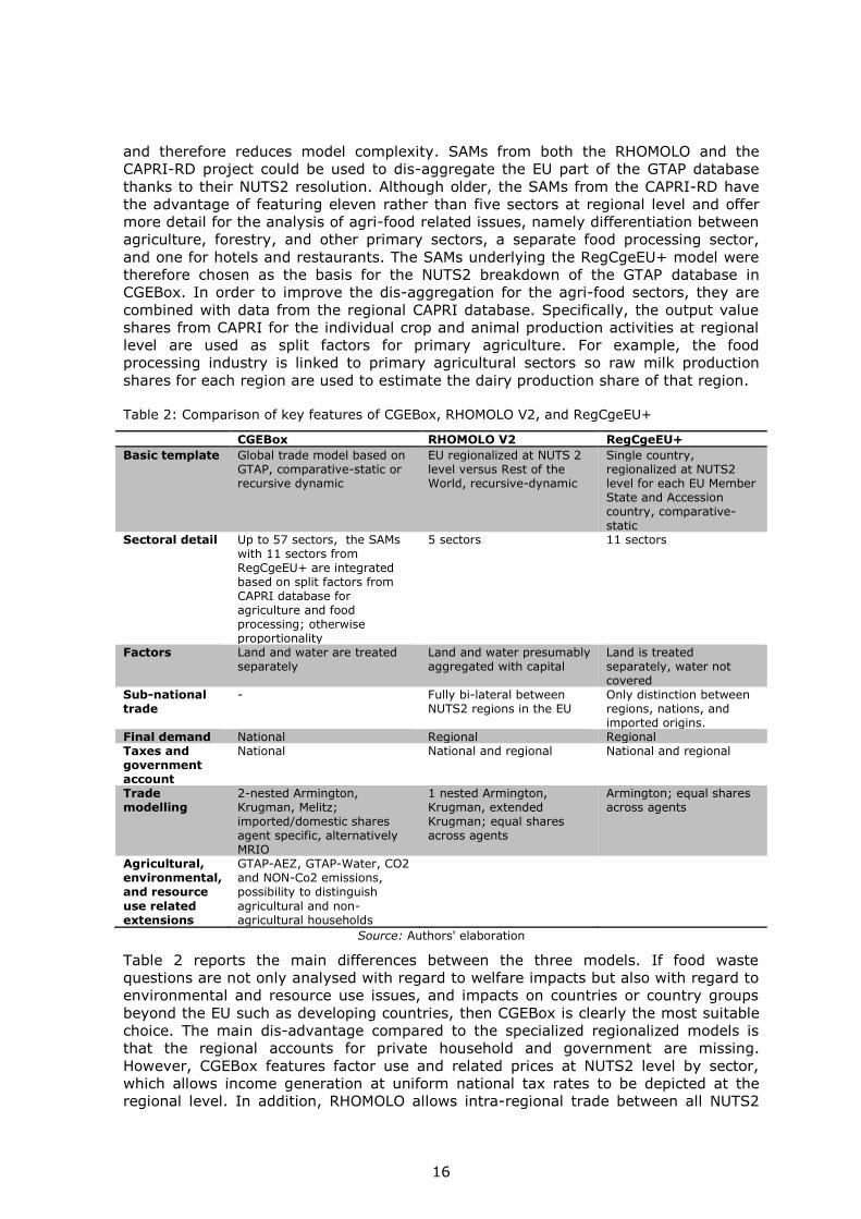
Table 2: Comparison of key features of CGEBox, RHOMOLO V2, and RegCgeEU+

CGEBox RHOMOLO V2 RegCgeEU+

Basic template Global trade model based on GTAP, comparative-static or recursive dynamic

EU regionalized at NUTS 2 level versus Rest of the World, recursive-dynamic

Single country, regionalized at NUTS2 level for each EU Member State and Accession country, comparative-static

Sectoral detail Up to 57 sectors, the SAMs with 11 sectors from RegCgeEU+ are integrated based on split factors from CAPRI database for agriculture and food processing; otherwise proportionality

5 sectors 11 sectors

Factors Land and water are treated separately

Land and water presumably aggregated with capital

Land is treated separately, water not covered

Sub-national trade

- Fully bi-lateral between NUTS2 regions in the EU

Only distinction between regions, nations, and imported origins.

Final demand National Regional Regional Taxes and government account

National National and regional National and regional

Trade modelling

2-nested Armington, Krugman, Melitz; imported/domestic shares agent specific, alternatively MRIO

1 nested Armington, Krugman, extended Krugman; equal shares across agents

Armington; equal shares across agents

Agricultural, environmental, and resource

use related extensions

GTAP-AEZ, GTAP-Water, CO2 and NON-Co2 emissions, possibility to distinguish

agricultural and non-agricultural households

Source: Authors' elaboration

Table 2 reports the main differences between the three models. If food waste

questions are not only analysed with regard to welfare impacts but also with regard to

environmental and resource use issues, and impacts on countries or country groups

beyond the EU such as developing countries, then CGEBox is clearly the most suitable

choice. The main dis-advantage compared to the specialized regionalized models is

that the regional accounts for private household and government are missing.

However, CGEBox features factor use and related prices at NUTS2 level by sector,

which allows income generation at uniform national tax rates to be depicted at the

regional level. In addition, RHOMOLO allows intra-regional trade between all NUTS2

17

regions in Europe to be depicted, while CGEBox only depicts bi-lateral trade at the

level of nations, it allows dis-aggregation of the non-EU countries into many countries

or country blocks.

3.4 Market structures

3.4.1 Options to depict international trade in CGEBox

CGEBox allows international trade to be depicted based on four different

methodological choices. The Armington assumption as the first option is the most

commonly used, differentiating products by region of production, i.e. origin, using a

CES-utility function. All major CGE models use at least a two-stage Armington system

with different substitution elasticities between the domestic and import origin and

between individual importers. However, they differ in terms of differentiation by

agent. By way of example, in the GTAP Standard model, the shares in the top-level

nests are agent specific, i.e. different for each production sector and each final

aggregate demand agent. The second example, GLOBE, removes that differentiation

completely. However, the GTAP database does not offer agent specific bi-lateral trade

shares. This data, named Multi-Regional Input-Output (MRIO), is to some degree

available in CGEBox thanks to shares provided by the METRO model of the OECD.

CGEBox offers the choice of using the GTAP standard layout, where the different

Armington agents (production sectors, private household, government, savings) have

different import and domestic shares, or the GLOBE layout where all these shares are

identical, or intermediate solutions. The MRIO extension aggregates all intermediate

demanders, but also uses agent specific shares for the bi-lateral trade relations. A

frequent complement to the Armington assumption is the use of identically structured

CET nests to distribute supply, an option also supported by CGEBox.

A not widely used option to depict international trade in CGE models is the use of the

Krugman and Melitz approaches, both available in CGEBox. MIRAGE is the only well-

known CGE model employing the Krugman formulation. It has been widely used for

impact assessment of trade policy in studies for the EU Commission. While Krugman

assumes fixed costs for a firm entering a sector, Melitz expands the model through

trade link specific fixed costs. The resulting decreasing constant returns to scale,

which would favour the emergence of monopolies, and is offset by assuming intra-

sectoral product differentiation leading to firm specific prices, love of variety by the

consumers as well as productivity distribution across firms. Introducing these features

leads to additional mechanisms not depicted by the Armington model. By way of

example, bi-lateral trade liberalisation allows less productive firms to start trading,

benefitting consumers because more varieties are available, while the expansion of bi-

laterally traded quantities distributes the fixed costs of trade over larger quantities.

Opposite impacts are observed in the domestic market following the increased

competition from imports. The Melitz extension of CGEBox is explained in Jafari and

Britz (2018).

3.4.2 Default market structure for the current project

The default configuration for CGEBox for the current project is based on the

extensions explained below. With regard to international trade, all markets use the

MRIO extension, i.e., bi-lateral import shares differ between intermediate demand,

government demand, final demand, and investment. An aggregation of intermediate

demand in the top level nests fits that formulation so imported and domestic shares

are identical across the sectors.

This also helps to reduce the numerical complexity related to the application of the

Melitz extension (for details on the Melitz extension, see http://www.ilr.uni-

18

bonn.de/em/rsrch/CGEBox/GTAP_Melitz.pdf) which is applied to five food processing

sectors (cattle meat, other meat, dairies, beverages and tobacco, other food industry)

and five industrial sectors (textiles and apparel, chemicals, petroleum and coke, light

manufacturing, and heavy manufacturing) and one service sector (Trade, which is

mostly retail). Sugar, rice, and oilseed processing as well as leather processing are

depicted as competitive sectors as are all primary and all services, with the exception

of the so-called trade service sector which includes retail and wholesale in the GTAP

database. Following the set-up by Akgul et al. (2016), the Melitz extension introduces

a separate fixed cost nest, with a higher share of value added. The shape parameter

of the Pareto distribution of firm productivity is chosen as 4.6. The two-stage

Armington configuration is used for all competitive sectors, which is complemented by

a two-stage CET (Constant Elasticity of Transformation) approach which distributes

regional output to the domestic market and exports (first stage) and to the various

export destinations (second stage).

3.5 Production function nesting and factor supply

CGE models such as the GTAP Standard model, GLOBE, or MIRAGE make different

assumptions about the degree to which inputs can be substituted against each other

and basically completely relies on nested CES functions (see Table 3 below). Variants

of GTAP such as GTAP-E introduce additional nests. CGEBox supports a flexible nesting

approach based on sets definitions, which also eases the task of replicating more

complex nesting structures without the need to add equations and variables manually.

A similar approach based on nested CET structures is also available for factor supply.

Table 3: Overview of production function nesting in the different models

Production function nesting

Model Value Added – Intermediate

composite

Intermediate composite

Value Added

GTAP Standard

Leontief Leontief CES

GLOBE Leontief CES CES, with sub-nest for skilled/unskilled labour

MIRAGE Leontief CES CES, with capital-skilled labour sub-nest ENVISAGE CES CES with sub-nests

for energy CES, skilled-unskilled labour nest

Source: Authors' elaboration

The default production function configuration of CGEBox in the current study is

composed of the following structure:

1. The intermediate and value added can be substituted against each other

(“gams\parameters\ND_VA.gms”) with moderate elasticity.

2. The same holds for inputs inside the intermediate nests

(“gams\parameter\IO_SUBS.gms”).

3. Intermediates classified as feed inputs into livestock activities can be

substituted more easily against each other as part of the GTAP-AGR module.

The same holds for agricultural inputs into the food processing sectors.

4. According to GTAP-E, there is multi-level nesting structure for energy

intermediates. The top level nests substitute energy against capital as a sub-

nest of the Value Added composite.

5. As part of GTAP-E, skilled and unskilled labour are considered to be partial

substitutes.

19

6. The fixed costs of production and trade depicted in the Melitz model, i.e. for

non-competitive sectors, comprise a higher share of primary factors compared

to the variable ones. However, the intermediate composite in the fixed and

variable cost nests share the nestings described in points 1-5 above.

The following defaults are used for factor supply:

1. Natural resources are assumed to be immobile.

2. According to the capital vintage module, non-depreciated capital is

considered immobile and newly formed capital is mobile.

3. For all primary factors, including new capital, there is sluggish factor supply

between agricultural and non-agricultural sectors as part of GTAP-AGR at

national level.

4. Land and water are considered regionally immobile in the NUTS2 module

whereas the other factors are considered to be sluggish when moving between

regions within a nation.

5. In addition, land cannot move across Agro-Ecological Zones (AEZ) according to

the GTAP-AEZ module, and NUTS2 regions are broken down AEZs.

Furthermore, GTAP-AEZ introduces a nested CET-approach to land in different

agricultural uses.

6. Irrigation water supply is assumed to be sluggish (see

“gams\extenions\water_nest.gms”).

Factors stocks at the national level and, where applicable at regional level, are

considered to be fixed. The only exceptions are: (1) irrigation water in non-water-

constrained regions (see the next chapter for a detailed discussion), (2) new capital,

which is equal to gross investments according to the capital vintage module.

3.6 Database detail and configuration

The database is set up as follows:

Based on GTAP9-Water, i.e., water as separate primary factor and the

distinction between irrigated and non-irrigated production activities.

25 single EU member States plus a residual aggregate, 9 regional aggregates

for non-EU regions: North America, Latin America, Middle East and North

Africa, Sub-Saharan Africa, East Asia, Southeast Asia, South Asia, Oceania, and

the Rest of the World.

Full sectoral detail for agriculture (including irrigated/non-irrigated

distinction; paddy rice, wheat, other grains, oilseeds, fruit and vegetables,

sugar beet/cane, fibre crops, other crops, ruminants for cattle, raw milk, wool,

other animal products) and food processing (ruminant meat, other meat,

dairy products, paddy processing, sugar, oilseed processing, other food

industry, beverages, and tobacco).

Remaining sectors highly aggregated, but with some important detail for the

bio-economy (leather, textiles, lumber) and as intermediate providers to

agriculture (chemicals, coke, and petroleum).

Non-diagonal make to remove the split-up in irrigated/non-irrigated

commodities found in GTAP-WATER, but keeping irrigated/non-irrigated

activities dis-aggregated.

Moderate filtering of raw GTAP-AGG output (1.E-10 absolute, 1.E-5% relative).

The 21 EU regions (Finland, Sweden, Denmark, United Kingdom, Ireland,

Germany, Netherlands, Belgium, France, Austria, Spain, Portugal, Italy,

Greece, Poland, Bulgaria, Romania, Slovakia, Slovenia, Czech Republic,

Hungary) which comprise NUTS2 data are dis-aggregated regionally to NUTS2;

20

Other EU countries in the dataset as single countries are: Estonia, Latvia,

Lithuania, Croatia; remaining EU28 aggregate: Cyprus, Malta, Luxembourg.

GTAP-AEZ breakdown also implemented for NUTS2 regions, using land use

information from CAPRI regional data and some GIS work.

NUTS2 SAMs (originally comprising only one agricultural sector) enriched by

data on regional production value of agricultural activities from CAPRI

database; meat, sugar, paddy rice and milk processing linked to related

primary agricultural production value at regional level.

Other details in the configuration:

Accounting for CO2-Emissions and Non-CO2 Emissions

MyGTAP: Distinction between agricultural and non-agricultural households,

based on factor income shares; separate government account

Post-model aggregation to continents and EU28; crops/animals/food

processing/all industry sectors

Trade in VA indicators based on calculating the global Leontief inverse

3.7 Closures and numeraires

As in GTAP standard, i.e.:

Fixed exchange rate as regional numeraire

Global factor prices index as world numeraire (Walras’ law)

Private household and government adjust spending

Global bank mechanism closing trade balance

A separate closure file (“gams\scen\closures\water.gms”) defines a list of NUTS2

regions where irrigation water is not judged to be constrained so that it is not a fixed

stock, but a fixed price is introduced. For details on modelling water, see section

“Natural resources and environmental accounting”.

3.8 Model size and solution strategy

CGEBox offers some flexibility on how to solve the model. The current project used the

following options.

Global scaling factor for GTAP database 1000

Minimal scaling factor for variables in model is 1.E-3

1 round of pre-solves for single countries, in memory grid parallel

(Solvelink=6)

No intermediate solve of trade side; only Full model solved as a CNS in

CONOPT4 (parallel)

Armington quantities (but not prices) are substituted out, import/domestic

prices are substituted out

The resulting model size is about 505,000 equations and variables. This model takes

about 6.5 minutes to find the solution on a Laptop with an Intel I7-6500U CPU @2.5

GHZ and 8 GB RAM using GAMS 25.0, of which 3 minutes are spent on post-model

processing. Time spent increases considerably when the global Leontief inverse for the

Trade in Value Added (TiVA) extension and related indicators are calculated.

3.9 Natural resources and environmental accounting

Natural resources are accounted for in CGE/IAM models (Integrated Assessment

Models) in various ways. As primary resources, their rent enters the value added of

some resource dependent industries and their availability constrains the supply. For

instance, endowments of natural resources are indirectly estimated in the GTAP

database on the basis of given industry supply elasticities. Secondly, some natural

21

resources are “hidden” production factors because they are not marketed and their

contribution cannot be properly assessed on the basis of economic accounts. Finally,

natural resources are affected in various ways by economic activities and it is often

important to evaluate the “footprint” of the economy on the environment. From the

modelling perspective, environmental data complement the economic, but

environmental variables do not affect the general equilibrium unless markets for

primary resources are created as part of a policy.

A thorough discussion of the modelling of natural resources is beyond the scope of this

report. The following briefly illustrates two specific cases and how they are

implemented in CGEBox: water and greenhouse gas emissions. These two cases are

representative of non-marketed factors (water) and auxiliary variables with possible

inclusion in the market functioning (emissions).

3.9.1 Water

Calzadilla et al. (2016) discuss the issue of modelling water resources in CGE models

in full. In essence, two main approaches are found in the literature. One approach

interprets water as an implicit factor, whose availability is reflected in variations of the

total factor productivity, especially in agriculture. The second approach elicits a price

for water as part of the value and rent of land. These two approaches are somewhat in

line with two water management schemes: the first is consistent with water

interpreted as a public, non-market good (prevalent in Europe) whereas the second is

more coherent with the so-called “riparian doctrine” for water rights (prevalent in the

U.S.A.). At the moment, the second methodology is implemented in CGEBox although

there are in principle no major difficulties in considering exogenous variations in

productivity.

Data on irrigated agriculture is provided by a special version of the GTAP9 database

termed “GTAP-Water” (Haqiqi et al., 2016). For the purposes of CGEBox, the so-called

diagonal version of the database is used, which can be aggregated by GTAPAgg. That

version not only splits crop activities into irrigated and non-irrigated ones, but also the

related outputs, thus not only differentiating “irrigated wheat” from “non-irrigated

wheat” in production, but also in demand and trade. It is therefore recommended that

the aggregation facility built in the data driver of CGEBox to aggregate the irrigated

and non-irrigated commodity back into one category is used so the distinction

between rainfed and irrigated in the model is only found at the production stage.

The integration of irrigation water into CGEBox has been enhanced by the project for

the NUTS2 resolution in two ways. Firstly, data on irrigated areas at NUTS2 level from

Eurostat is integrated in the construction of the NUTS2 SAMs. When the GTAP-Water

database was used in the past, the national share of irrigated and non-irrigated crops

in the total output found in the SAM was used to split the estimated regional output

based on CAPRI data. In contrast, these shares now reflect the regional data from

Eurostat which are stored in GAMS format under

“gams\GTAPNuts2\NUTS2_irr_area.gms”.

Secondly, a distinction between water stressed and non-water stressed regions has

been introduced. In the latter case, it is assumed that the amount of irrigation is

currently not limited, which implies infinite supply elasticity. The price for these

regions is fixed at a benchmark level. For the other regions, available irrigation water

is treated as a fixed stock so endogenous price adjustments ensure market clearing.

This option can be activated as an additional closure file, and the list of water stressed

regions is found under “scen\closures\water.gms”.

22

3.9.2 GHG Emissions

GTAP offers data on emissions for carbon dioxide (CO2) and Non-CO2 as part of two

different satellite accounts. The so-called GTAP-E database provides CO2 emissions

data distinguished by fuel and by user for each of the 140 countries/regions in the

GTAP9 Data Base. The GTAP-E database was already integrated into the data driver of

CGEBox before the project started so the related emissions are integrated as

equations in the modelling framework. This means that these emissions can be taxed,

or the functioning of an emissions’ rights market can be simulated, which affects the

general equilibrium state.

The GTAP Non-CO2 Emissions database is now available, providing information on

other greenhouse gas (GHG) emissions such as Methane (CH4), Nitrous Oxide (N2O),

and Fluorinated gas (FGAS). These sources of climate relevant gases are of special

interest for agriculture. Agricultural production activities account for a larger share of

Methane emissions in many countries, linked to paddy rice production and enteric

fermentation from ruminants while Nitrous Oxide is linked to the use of mineral and

organic fertilizers. So far, the Non-CO2 emissions are only used for post-model

reporting and have not been integrated in the equation system of the model yet. This

means that endogenous or policy-driven variations in Non-CO2 emissions have no

effect on the general equilibrium of the economy.

3.10 Trade in Value Added (TiVA)

The TiVA extension implements a well-established framework drawing on the Leontief

multiplier analysis into the post-processing of CGEBox in order to assess the income-

generating role of exports and to attribute sectoral outputs to final demand. Appendix

A details how the TiVA extension, developed in the context of the project, is

implemented in the GAMS code of CGEBox.

Trade has a dual role. First, it allows consumers to choose between domestically

produced goods and imports; second, it offers income opportunities by means of

exports. The first role is traditionally assessed in a CGE framework by reporting import

shares on demand. The second role is reflected in the accounting identity for GDP by

the difference between exports and import values, i.e. the balance of trade.

However, with the rapid increase in Global Value Chains (GVCs) and in intermediate

trade flows, import shares, domestic and export shares are no longer a good indicator

of the underlining sourcing. Domestic production comprises imported intermediates

which generate income abroad. As a matter of fact, gross imports are not entirely

foreign sourced and include some portion of domestic value added, which is imported

back after further processing stages abroad (Daudin et al., 2011; Koopman et al.,

2014). In the same way, export revenues comprise both domestic and foreign value

added embedded in domestic and foreign intermediates.

The TiVA extension in the CGEBox introduces the decomposition of gross trade flows

(as reported by standard trade statistics) in terms of value added content (for

example, see Johnson and Noguera, 2012; Foster-McGregor and Stehrer, 2013; Wang

et al., 2013; Koopman et al., 2014; Borin and Mancini, 2015). Specifically, it

distinguishes between the domestic and the foreign value added. The domestic VA

content of exports provides a measure of the contribution a given export makes to an

economy’s income, the remainder being the value of imported inputs representing the

import content of exports or vertical specialization (Hummels et al., 2001). At sector

level, it allows the value added originated in one (domestic or foreign) sector and

exported by another sector to be calculated.

Finally, the decomposition of each sector's contribution to final demand facilitates the

calculation of the output from each sector which is directly or indirectly (e.g.,

23

embedded as input in other intermediates used in the production of final goods)

embedded in the final consumption.

The main indicators of the value added/output content of trade and final demand are

summarized in Table 4. These are the first steps in modelling GVC-related trade and

production within a CGE context and this framework is also forms the basis for a

footprint analysis or for attributing environmental externalities linked to factor or

output use to final demand. Further extensions would allow the foreign country of

origin of value added in exports at the bilateral level to be disentangled, and the

domestic and foreign portions of output for each sector to be distinguished.

Table 4: Indicators of Trade in Value Added in CGEBox

Indicator Description

tradeInVaM Value added multipliers tradeInVa Domestic and foreign value added content of trade QTiva Final demand decomposition in terms of sector contributions

Source: Authors' elaboration

24

4 Quantitative results

4.1 General considerations

The general impacts expected from reducing food waste in the European food industry

are the following: as intermediate demand for primary agricultural products falls,

supply and prices for agricultural products will decrease and, consequently, returns to

agricultural primary factors will also fall, leading to loss of income for farmers.

Reduced demand for land and irrigation water as well as less intensive agricultural

production practices may lead to environmental quality improving. However, since the

food industry needs other resources to reduce food waste, these could drive up the

demand for such things as fossil fuel resources, with negative environmental impacts.

CGEs do not treat primary agricultural products as perfect substitutes, and the

consequences vary in different regions/countries. One aim of reducing food waste is to

increase food security. Food security is both a question of regional food availability

and of being able to afford food, which depends on income and food prices. The

impacts here are ambiguous. Dropping agricultural prices reduces the farmer’s income

and therefore farmers' purchasing power but leads to cost savings in the Rest-of-the-

World’s food industry, which should decrease the price of processed food. However,

under the assumption that reducing food waste is not cost-neutral, European food

processors will become less competitive so European net exports of processed food

will decrease, countervailing the positive impact on global food security from reduced

demand for agricultural products in Europe and cost savings in the Rest-of-the-World

food industry.

4.2 Standard configuration

The reader is reminded that the so-called “Standard configuration” in CGEBox is not

the Standard GTAP model but a rather complex configuration of CGEBox in which the

MRIO and the Melitz model, GTAP-AEZ, GTAP-AGR with an agricultural and non-

agricultural household, and the NUTS2 resolution for Europe are all combined (see

Section 3).

4.2.1 Welfare and income effects

At the global level, the impacts on agricultural prices of a cost-neutral 5% reduction in

agricultural input of the European food industry (Cost Neutral Scenario) are very

minor. That simply reflects the fact that the European food industry does not

represent a large share of the global agricultural products demand. Global prices for

primary agriculture products and food processing drop by -0.2% and -0.12% on

average, respectively. However, the price drops are larger in the EU. For example, the

drop for agricultural products is around -0.7% for crops and -2% for animals,

respectively. Owing to stronger reliance on domestic products, the price per household

in Sub-Saharan Africa shows a very small increase.

The price changes in the Europe Union differ between the Member States. Price drops

can be as large as -4% across the EU. There is no single explanation of differences in

price drops between Member States, which depend inter alia on the demand

composition of the food industry and its sourcing from domestic and imports. Animal

products have a tendency to show larger drops which reflects the fact that most

slaughtering and meat processing is closer to the point of production compared to food

processing of crops. This implies greater reliance on domestic output while exports of

primary agricultural outputs play a very minor role in most cases, especially beyond

(neighbouring) EU countries. This means that the domestic market of animal outputs

has to absorb the reduction in input use by the food processing industry to a large

extent.

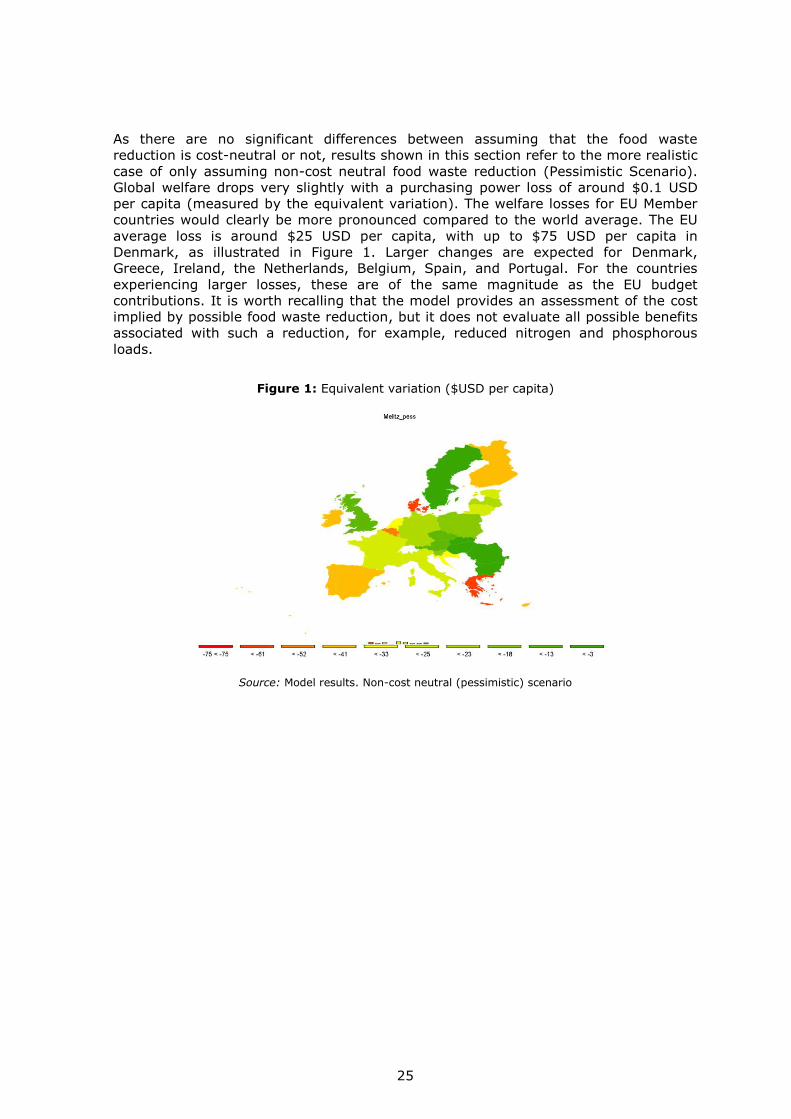
25

As there are no significant differences between assuming that the food waste

reduction is cost-neutral or not, results shown in this section refer to the more realistic

case of only assuming non-cost neutral food waste reduction (Pessimistic Scenario).

Global welfare drops very slightly with a purchasing power loss of around $0.1 USD

per capita (measured by the equivalent variation). The welfare losses for EU Member

countries would clearly be more pronounced compared to the world average. The EU

average loss is around $25 USD per capita, with up to $75 USD per capita in

Denmark, as illustrated in Figure 1. Larger changes are expected for Denmark,

Greece, Ireland, the Netherlands, Belgium, Spain, and Portugal. For the countries

experiencing larger losses, these are of the same magnitude as the EU budget

contributions. It is worth recalling that the model provides an assessment of the cost

implied by possible food waste reduction, but it does not evaluate all possible benefits

associated with such a reduction, for example, reduced nitrogen and phosphorous

loads.

Figure 1: Equivalent variation ($USD per capita)

Source: Model results. Non-cost neutral (pessimistic) scenario

26

Figure 2 highlights that changes in value added would mostly affect the peripheral regions of the EU. While most regions are expected to be affected negatively, some are likely to experience a small but positive change, reaching 0.13% in a few regions. The few positive impacts disappear when only the impact on

agricultural value added, of both crop and animal production, is focussed on. As shown in Source: Model results. Non-cost neutral (pessimistic) scenario

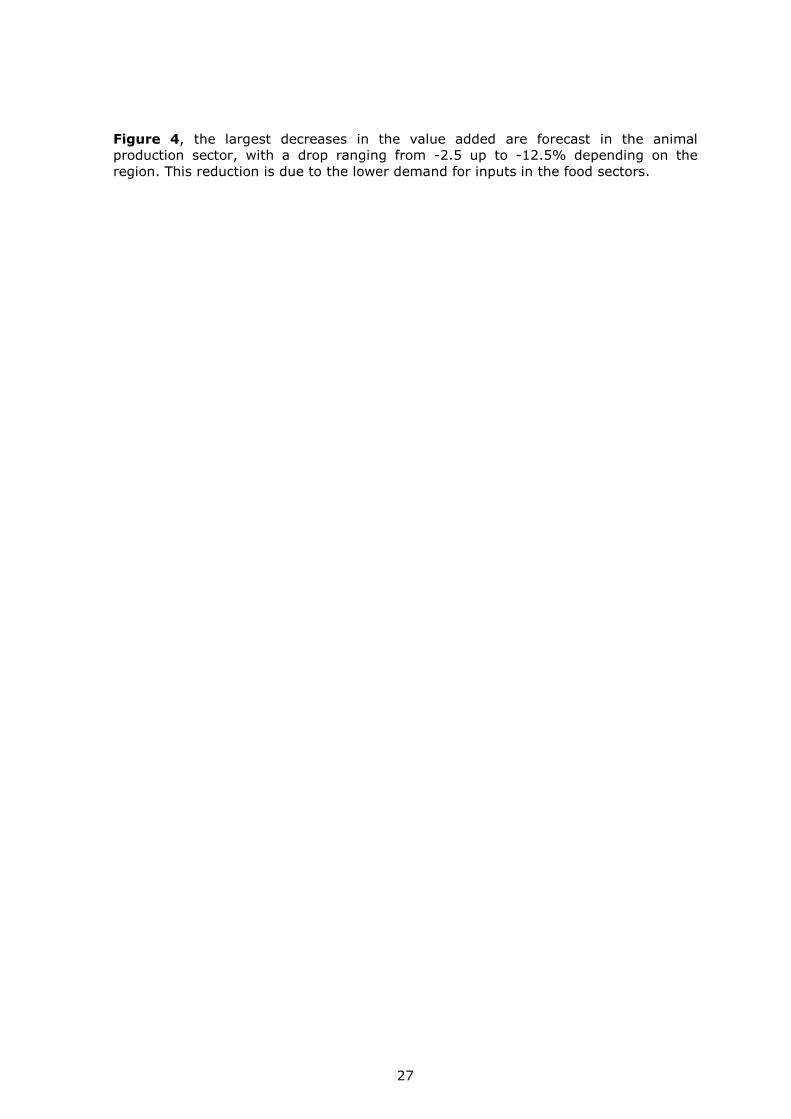
27

Figure 4, the largest decreases in the value added are forecast in the animal

production sector, with a drop ranging from -2.5 up to -12.5% depending on the

region. This reduction is due to the lower demand for inputs in the food sectors.

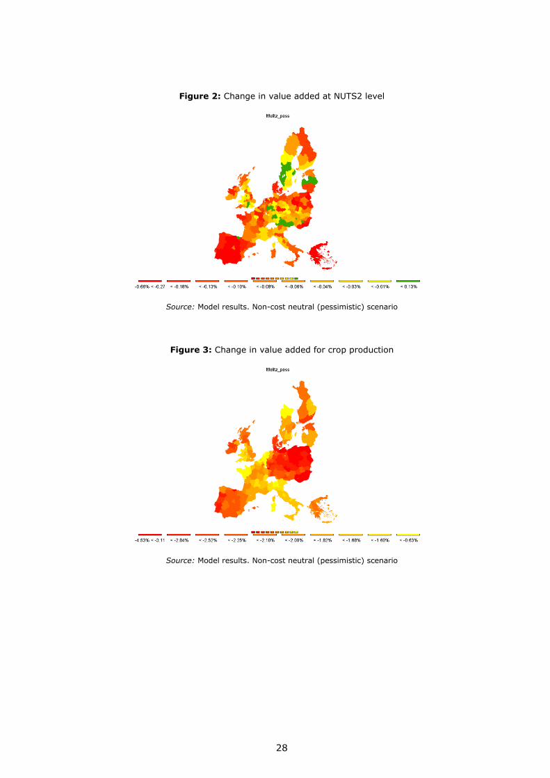
28

Figure 2: Change in value added at NUTS2 level

Source: Model results. Non-cost neutral (pessimistic) scenario

Figure 3: Change in value added for crop production

Source: Model results. Non-cost neutral (pessimistic) scenario

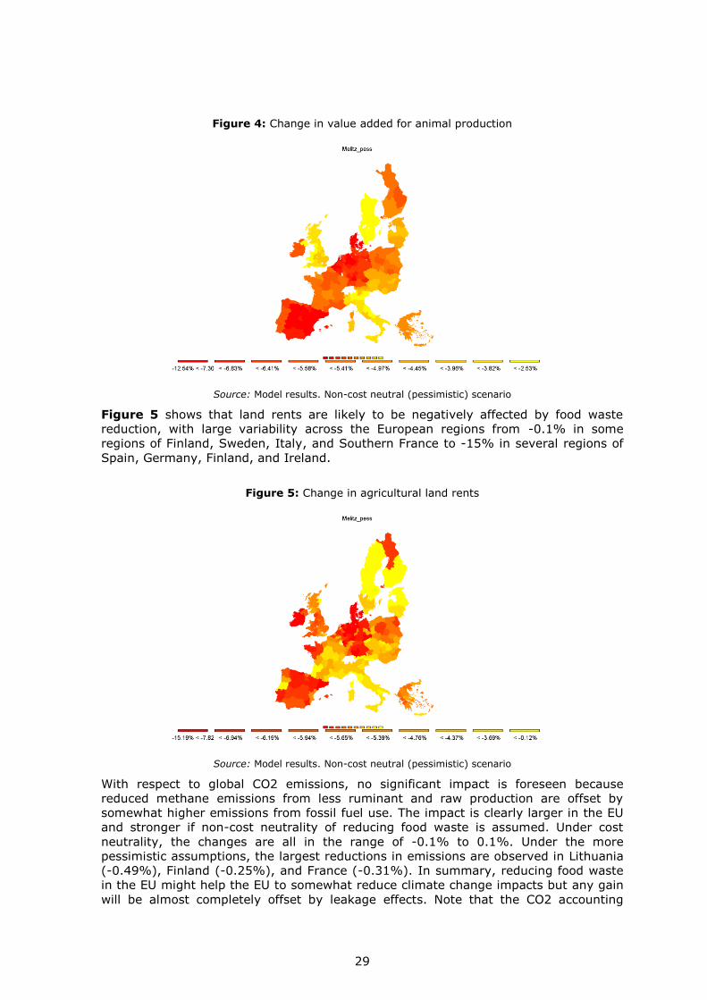
29

Figure 4: Change in value added for animal production

Source: Model results. Non-cost neutral (pessimistic) scenario

Figure 5 shows that land rents are likely to be negatively affected by food waste

reduction, with large variability across the European regions from -0.1% in some

regions of Finland, Sweden, Italy, and Southern France to -15% in several regions of

Spain, Germany, Finland, and Ireland.

Figure 5: Change in agricultural land rents

Source: Model results. Non-cost neutral (pessimistic) scenario

With respect to global CO2 emissions, no significant impact is foreseen because

reduced methane emissions from less ruminant and raw production are offset by

somewhat higher emissions from fossil fuel use. The impact is clearly larger in the EU

and stronger if non-cost neutrality of reducing food waste is assumed. Under cost

neutrality, the changes are all in the range of -0.1% to 0.1%. Under the more

pessimistic assumptions, the largest reductions in emissions are observed in Lithuania

(-0.49%), Finland (-0.25%), and France (-0.31%). In summary, reducing food waste

in the EU might help the EU to somewhat reduce climate change impacts but any gain

will be almost completely offset by leakage effects. Note that the CO2 accounting

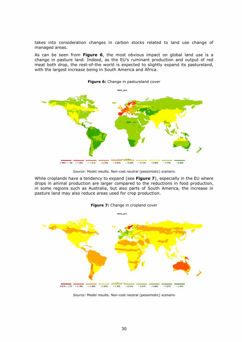
30

takes into consideration changes in carbon stocks related to land use change of

managed areas.

As can be seen from Figure 6, the most obvious impact on global land use is a

change in pasture land. Indeed, as the EU’s ruminant production and output of red

meat both drop, the rest-of-the world is expected to slightly expand its pastureland,

with the largest increase being in South America and Africa.

Figure 6: Change in pastureland cover

Source: Model results. Non-cost neutral (pessimistic) scenario

While croplands have a tendency to expand (see Figure 7), especially in the EU where

drops in animal production are larger compared to the reductions in food production,

in some regions such as Australia, but also parts of South America, the increase in

pasture land may also reduce areas used for crop production.

Figure 7: Change in cropland cover

Source: Model results. Non-cost neutral (pessimistic) scenario

31

Finally, he differentiated impact of a unilateral effort by the EU to reduce food waste

can be clearly seen in the change in managed forest areas. Reduced demand for

agricultural products in the EU releases pressure on crop and pasture land, which in

the long run would lead to a certain extent of new afforestation. The opposite is true

outside the EU, where pressure on the tropical rainforest would increase.

Figure 8: Change in managed forest land cover

Source: Model results. Non-cost neutral (pessimistic) scenario

The CGE modelling system does not (yet) track nitrate and phosphate balances as

found in Multi-Commodity models, such as CAPRI. However, the reduced crop (-1%)

and animal output per unit of land (-3%) found in the simulation shows an

extensification effect, which can also be seen from the fact that total intermediate

input use per unit of land drops by around -2% in crop and -4.3% in animal

production.

4.3 Alternative model configurations

4.3.1 Trade specification

The following table shows the EV per capita results under different modelling options

for international trade. As expected, the largest changes are in the Melitz extension.

There is general agreement on the direction of the change, with only two exceptions.

All configurations also show larger losses for Oceania, Spain, and Hungary.

Interestingly, average changes for EU28 as a whole are rather limited, but differences

between Member States are far larger. By way of example, despite the higher

differences in the EV, simulated changes in land prices are rather similar for the

various configurations of international trade.

32

Table 5: EV per capita under different trade configurations

Melitz-MRIO Melitz ArmStd _CET ArmStd

World 0.22 0.22 0.09 0.08 Australia, New Zealand -1.59 -1.63 -2.09 -2.23 Rest of World 0.52 0.49 0.19 0.26 Middle East and Africa 0.15 0.16 0 0.06 Asia 0.02 0.02 0 0.01 America -0.5 -0.47 -0.63 -0.67 EU28 3.16 312 2.46 2.13 Austria 8.84 9.21 5.58 5.54 Belgium 9.19 9.33 7.64 6.01 Germany 4.38 4.25 4.4 3.93 Czech Republic -0.1 -0.1 1.27 0.66 Denmark 15.94 16.89 0.13 -0.85 Spain -3.35 -3.28 -1.44 -1.62 Estonia 23.09 22.9 7.01 6.92 Finland 3.56 5.35 4.47 3.67 France 4 4.23 1.79 1.74 Greece 3.07 3.33 3.29 2.57 Hungary -1.47 -0.99 -2.45 -3.15 Ireland 7.95 7.12 -4.19 -2.43 Italy 2.11 2.33 3.09 2.59 Netherlands -5.3 -5.49 -7.85 -7.7 Poland 2.58 2.56 1.58 1.54 Portugal -0.06 0.02 3.22 2.75 Sweden 3.4 3.51 3.7 3.38 United Kingdom 6.99 6.85 6.11 5.73 Bulgaria -0.49 -0.55 -1.85 -1.82 Slovakia 2.21 2.69 1.86 1.56

Slovenia 4.59 3.75 1.32 1.33 Romania 6.54 6.49 4.04 3.77 Latvia -1.87 -1.82 0.34 -0.12 Lithuania 0.42 0.33 -0.42 -0.62 Croatia 1.19 0.8 0.96 1.18 Rest of EU28 0.67 1.19 4.53 2.64

Source: Model Results. Non-cost neutral (pessimistic) scenario

As can be seen from Table 6 below, the difference between the Melitz and the

Armington specifications can have significant impacts on results. The Armington

formulation increases global trade significantly in relative terms, and almost all

additional output is exported. In the Melitz model, increasing demand implies two

opposing effects: distributing the fixed trade costs on larger quantities, which

decreases costs, and letting less competitive firms enter the market, which increases

costs. The net effect here is to reduce the increase in trade.

Interestingly, there is an increase in the global demand for food-processing products

under the Armington configuration and the scenario where cost-neutrality at

benchmark prices is assumed. As prices for agricultural inputs drop due to the

assumed reduction in input demand per unit of output in the food industry, the food

industry becomes more competitive and increases its output. Note that this implies a

contribution to global food security as even in many developing countries the main

staple foods such as bread stem from food processing.

Table 6: Global demand for food-processing products

ArmStd ArmStd CET

Melitz Melitz MRIO

Total 12312 12312 12123 12122 1.69% 1.70% 0.13% 0.13% Domestic 10637 10637 10645 10644 0.05% 0.05% 0.13% 0.12% Imported 1675 1675 1478 1478 13.54% 13.56% 0.19% 0.17%

Source: Model Results. Non-cost neutral (pessimistic) scenario

33

4.3.2 Trade in value added

The TiVA extension allows some interesting additional results to be obtained. As

previously mentioned, food waste reduction leads to a reduction in EU food-processing

output largely because of the contraction in exports. The demand for crops and animal

agricultural inputs from the food sector decreases accordingly.

Looking at the demand side, Table 7 presents the change of the agricultural inputs

embedded in final consumption of food products for different markets in the

pessimistic scenario. The reduction differs from the 5% reduction in domestic

agricultural inputs used by the EU food industry simulated for two reasons. Since

calculations are based on global Leontief multipliers, they take into account both

domestic and imported agricultural inputs as well as agricultural inputs embedded in

intermediate goods produced by other sectors and used in food production. Even in

the case of the EU, i.e., the region directly hit by the shock, the reduction in the value

output from crops and animals is less than 5% (-2.12% and -1.70%, respectively).

However, there are large differences across the Member States: reductions in Belgium

exceed 4% while in Greece they are less than 1%.

Table 7: Primary agricultural output embedded in the final consumption of food products

Crops Animals

World 900.86 -0.25% 622.06 -0.57% Australia, New Zealand 5.03 -0.07% 8.46 -0.21% Rest of World 33.64 0.28% 31.67 0.14%

Middle East and Africa 97.76 -0.01% 70.66 -0.17% Asia 483.38 -0.03% 184.20 -0.35% America 183.84 -0.08% 206.23 -0.36% EU28 97.20 -2.12% 120.83 -1.70%

Austria 1.37 -1.98% 1.71 -1.14% Belgium 2.67 -4.02% 1.39 -4.42% Germany 23.91 -2.03% 20.34 -1,00% Czech Republic 1.90 -2.38% 1.53 -1.50% Denmark 0.93 -1.77% 1.21 -3.14% Spain 11.97 -2.09% 13.45 -1.83% Estonia 0.08 -3.35% 0.16 -3.40% Finland 0.65 -2.40% 1.57 -2.92% France 11.29 -2.38% 17.47 -2.95% Greece 3.70 -0.93% 4.13 -0.65% Hungary 1.44 -1.88% 2.53 -0.63% Ireland 0.60 -1.71% 1.30 -1.09% Italy 11.28 -2.01% 16.08 -1.77% Netherlands 1.71 -2.31% 3.94 -2.50% Poland 4.89 -1.70% 8.60 -2.22% Portugal 1.94 -2.72% 2.37 -2.57% Sweden 1.33 -2.30% 1.91 -1.27% United Kingdom 9.15 -1.72% 14.28 0.01% Bulgaria 0.43 -2.67% 0.62 -2.22% Slovakia 0.54 -2.73% 1.01 -1.95% Slovenia 0.12 -1.13% 0.29 -2.28% Romania 3.70 -2.93% 2.12 -2.41% Latvia 0.26 -1.36% 0.24 -2.77% Lithuania 0.50 -2.75% 0.72 -2.74% Croatia 0.64 -2.47% 1.08 -3.02% Rest of EU28 0.20 -2.66% 0.77 -4.87%

Source: Model Results. Non-cost neutral (pessimistic) scenario

The reduction in domestic agricultural inputs demand by the food sector in several EU

countries is compensated by foreign agricultural goods and by intermediates provided

by other sectors that also need agricultural inputs. Due to the shock, production of

food exports would require more inputs from other sectors of the economy (e.g.,

34

services and industry) which would increase their output and, consequently, their

intermediate demand of those primary agricultural inputs which are cheaper due to

the contraction of demand from the food industry.

The TIVA indicator is used to compute the domestic and foreign content for each

intermediate input in the production of processed-food exports. The impact of the food

waste reduction on agriculture and food exports is assessed by considering: i) the

domestic content of EU exports; ii) the EU’s direct exports (value added originating in

the domestic sector which is exported through the same sector’s exports; and iii) the

EU’s indirect exports (value added originating in the domestic sector and embedded in

the exports of another domestic sector).

Figure 9 shows that crop exports have the highest domestic value-added share

(greater than 90%). The EU’s exports of food and animal products are more reliant on

foreign inputs which represent around 12% of the total exported value.

Figure 9: The composition of the EU's exports in food and agricultural products (shares in gross exports)

a) Food processing b) Crops

c) Animals

Source: Model Results. Baseline

35

It is worth emphasizing that EU agricultural value added is also exported through food

exports. The value of domestic intermediate goods provided by different sectors is

presented in Table 8.

Table 8: Decomposition by sector of the domestic value added in food-processing exports (million USD)

Sector of origin of value added

Food processing 193.61

Crops 16.87

Animals 24.46

Mining and Extraction 2.64

Electric power sources 4.9

Industry 24.52

Services 66.24

Other 6.09

Total 339.33

Source: Model Results. Baseline

We find very different impacts under the two simulated assumptions, which lead us to

consider the results here for both scenarios. Figure 10 shows the impacts on the

domestic value added embedded in exports of processed food and primary products.

Under the pessimistic scenario, European exports of food products decrease as a

result of the decrease in competition. Such a reduction would carry through the crop

and animal sectors, though with a much smaller impact on the former. Interestingly,

the cost neutral scenario would lead to an increase in exported values but in this case

the positive impact does not carry through the primary sectors.

Figure 10: Impact by sector on the domestic value added in the EU's total exports (% change)

Source: Model Results. Scenarios

Next, we consider the impact on direct export, that is, the change in the exported

domestic value-added originating in the exporting sector (Figure 11). In other words,

we net the results presented in Figure 10 from the values for domestic intermediates.

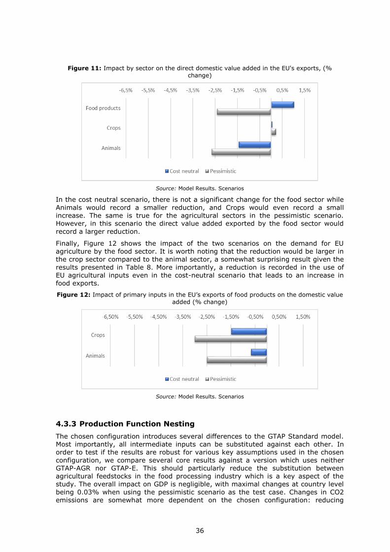
36

Figure 11: Impact by sector on the direct domestic value added in the EU's exports, (% change)

Source: Model Results. Scenarios

In the cost neutral scenario, there is not a significant change for the food sector while

Animals would record a smaller reduction, and Crops would even record a small

increase. The same is true for the agricultural sectors in the pessimistic scenario.

However, in this scenario the direct value added exported by the food sector would

record a larger reduction.

Finally, Figure 12 shows the impact of the two scenarios on the demand for EU

agriculture by the food sector. It is worth noting that the reduction would be larger in

the crop sector compared to the animal sector, a somewhat surprising result given the

results presented in Table 8. More importantly, a reduction is recorded in the use of

EU agricultural inputs even in the cost-neutral scenario that leads to an increase in

food exports.

Figure 12: Impact of primary inputs in the EU’s exports of food products on the domestic value

added (% change)

Source: Model Results. Scenarios

4.3.3 Production Function Nesting

The chosen configuration introduces several differences to the GTAP Standard model.

Most importantly, all intermediate inputs can be substituted against each other. In

order to test if the results are robust for various key assumptions used in the chosen

configuration, we compare several core results against a version which uses neither

GTAP-AGR nor GTAP-E. This should particularly reduce the substitution between

agricultural feedstocks in the food processing industry which is a key aspect of the

study. The overall impact on GDP is negligible, with maximal changes at country level

being 0.03% when using the pessimistic scenario as the test case. Changes in CO2

emissions are somewhat more dependent on the chosen configuration: reducing

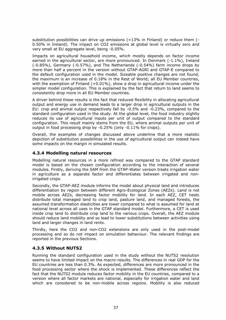
37

substitution possibilities can drive up emissions (+13% in Finland) or reduce them (-

0.50% in Ireland). The impact on CO2 emissions at global level is virtually zero and

very small at EU aggregate level, being -0.05%.

Impacts on agricultural household income, which mostly depends on factor income

earned in the agricultural sector, are more pronounced. In Denmark (-1.1%), Ireland

(-0.85%), Germany (-0.57%), and The Netherlands (-0.54%) farm income drops by

more than half a percent in the version without GTAP-AGRI and GTAP-E compared to

the default configuration used in the model. Sizeable positive changes are not found,

the maximum is an increase of 0.18% in the Rest of World; all EU Member countries,

with the exemption of Finland (+0.01%), show a drop in agricultural income under the

simpler model configuration. This is explained by the fact that return to land seems to

consistently drop more in all EU Member countries.

A driver behind these results is the fact that reduced flexibility in allocating agricultural

output and energy use in demand leads to a larger drop in agricultural outputs in the

EU: crop and animal output respectively fall by -0.5% and -0.23%, compared to the

standard configuration used in the study. At the global level, the food industry slightly

reduces its use of agricultural inputs per unit of output compared to the standard

configuration. This result mainly stems from the EU, where animal outputs per unit of

output in food processing drop by -0.25% (only -0.11% for crops).

Overall, the examples of changes discussed above underline that a more realistic

depiction of substitution possibilities in the use of agricultural output can indeed have

some impacts on the margin in simulated results.

4.3.4 Modelling natural resources

Modelling natural resources in a more refined way compared to the GTAP standard

model is based on the chosen configuration according to the interaction of several

modules. Firstly, deriving the SAM from the GTAP-Water version treats irrigation water

in agriculture as a separate factor and differentiates between irrigated and non-

irrigated crops.

Secondly, the GTAP-AEZ module informs the model about physical land and introduces

differentiation by region between different Agro-Ecological Zones (AEZs). Land is not

mobile across AEZs, decreasing factor mobility for land. In each AEZ, CET nests

distribute total managed land to crop land, pasture land, and managed forests, the

assumed transformation elasticities are lower compared to what is assumed for land at

national level across all uses in the GTAP standard model. Furthermore, a CET is used

inside crop land to distribute crop land to the various crops. Overall, the AEZ module

should reduce land mobility and so lead to lower substitutions between activities using

land and larger changes in land rents.

Thirdly, here the CO2 and non-CO2 extensions are only used in the post-model

processing and so do not impact on simulation behaviour. The relevant findings are

reported in the previous Sections.

4.3.5 Without NUTS2

Running the standard configuration used in the study without the NUTS2 resolution

seems to have limited impact on the macro-results. The differences in real GDP for the

EU countries are less than 0.3%. As expected, differences are more pronounced in the

food processing sector where the shock is implemented. These differences reflect the

fact that the NUTS2 module reduces factor mobility in the EU countries, compared to a

version where all factor markets are national, especially for irrigation water and land

which are considered to be non-mobile across regions. Mobility is also reduced

38

because additional CET-nests distribute mobile or sluggish factors from a national pool

to the regions.

At the EU28 level, the full model predicts a slight reduction in food processing output

by -0.07% whereas the same configuration without the NUTS2 extension forecasts an

increase of 0.34%. A lower increase or a sharper decrease, or a reduction instead of

an increase, is found for all Member States in the version with the NUTS2 extensions

compared to the version only modelling nations. Differences in total global CO2

emissions as an important externality are however negligible.

While using the NUTS2 extension clearly drives up solution time due to the larger

model size, it seems to provide robust results. As such, its use can probably be

recommended for all applications where (selected) NUTS2 results are of interest.

39

5 Conclusion

The project has three major aims: (1) to analyse the impacts of EU efforts to curb

food waste, (2) to test the CGEBox modelling system under policy relevant shocks and

(3) to improve CGEBox in selected areas.

Contrary to the other studies, it is not assumed here that a larger reduction of food

loss and waste is costless. Rather, two options are analysed: the first assumes cost-

neutrality at benchmark prices, whereas the second one assumes that reducing food

waste would incur additional costs. Food waste is assumed to be reduced in the food

industry only, and not by final demanders.

A unilateral commitment of the EU to reduce food loss and waste would most likely

decrease the competitiveness of the EU food processing. Reduced demand for primary

agricultural inputs would shrink the EU’s agricultural sectors, pressuring on farm

incomes and land prices. The contribution to global food security would be very minor,

as the adjustments would be concentrated in EU market. Rather, as many developing

countries are importers of both primary agricultural products and of processed food,

increasing global prices for processed food would harm them.

We could not find any significant impact on emissions relevant for climate change at

global level and only very limited contribution inside the EU.

With regard to testing CGEBox, the modelling systems showed its usefulness,

especially with regard to depicting outcomes at NUTS2 level and in quantifying global

land use impacts, based on GTAP-AEZ, while differentiating between irrigated and

non-irrigated crops. It was possible to maintain the full sectoral detail for agri-food as

found in the GTAP data base, despite the fact that all EU 28 Member countries were

considered by the analysis and a complex model configuration used. The application of

the Melitz module provides new insights about international trade, by considering the

impact of sector-wide and trade-link specific fixed costs, firm productivity distribution

and love of variety. CGEBox thus seems an interesting complement to other models

used for policy impact assessment; its modular and flexible concept renders it quite

versatile.

During the project’s lifetime, the modelling system was improved in several aspects.

The TiVA part was completely re-factored, and it is now based on the global Leontief

inverse and allows attributing production by trading partner to final demand, as well

as CO2 emissions. The NUTS2 layer was informed by data on regional irrigated areas

and a differentiation between water- and non-water stressed regions was introduced.

It was already noticed, in the introductory section, that there is no universal

consensus on the definition of “food waste” and that the concept may have alternative

interpretations. Therefore, in order to assess the significance and implications of the

numerical results obtained, it is essential to understand how “food waste” has been

interpreted here, and how the concept has been technically implemented into the

mathematical model.

The overall approach followed in this work is the one typical of mainstream economics,

which posits assumptions about preferences and rationality. First, we have refrained

from making any normative or “pedagogical” consideration about individual or social

preferences. This contrasts with the implicit moral judgement associated with the word

“waste”, recalling not only inefficiency, but also injustice and deprecated behaviour.

Second, rationality as assumed in model construction implies that the observed food

waste is the outcome of voluntary choices considered optimal by the individual making

that choice. In other words, observed waste must be, economically speaking, efficient

by construction. As a corollary: any departure from an optimal state must be costly, at

least in the aggregate.

40

Actually, it could well be possible that individual choices may not be socially optimal,

but this possibility has not been explored in this research, and for good reasons. This

may happen whenever social values do not coincide with private ones, so that

externalities and market failures emerge. For instance, suppose that consumers only

want perfectly rounded and red apples. You may say that discarding “imperfect” yet

fully eatable apples is a “waste”. But, from a scientifically neutral perspective, we do

not want to discuss why consumers have such preferences. Rather, the right questions

to pose are: is there a socially valuable use of “imperfect apples”? Why apple

producers choose to discard them? What kind of economic incentives can be offered to

realign individual behaviour with social objectives?

Coming more specifically to the numerical exercise illustrated in this report, it should

be noticed that a strategy of reduction of food waste has been interpreted here as a

change in the production technology of the food processing industry (in Europe). This

change in technology takes place by reducing the inputs of agricultural goods into food

processing, while scaling up the usage of all other production factors (in a cost neutral

or in a cost increasing way). Therefore, we have simulated an improved efficiency in

the utilization of agricultural goods, compensated by higher employment of all other

factors.

This compensation mechanism deserves some discussion. First, suppose that no such

compensatory change occurs. In this case, the reduction of food waste in the

processing industry would be a pure efficiency gain. This means that you could

produce more with the same resources, or that you would need fewer resources to get

the same output. But if that gain can be easily grasped, why has it not yet been

obtained? Agents cannot be rational, profit-maximizers and at the same time selecting

the “wrong” technology which is wasting inputs.

If we exclude that “manna from heaven” case, then there must be some

implementation costs. Which costs? Here, it is difficult to make any valuation without

specifying in detail which measures would be taken to reduce the gross amount of

agricultural inputs utilized. Remember that the model employed here is a

macroeconomic one, meaning that behind industries and households there are millions

of individuals and firms. As a consequence, there is no practical way to get any

realistic estimate of implementation costs for waste reduction programs

(disaggregated by industrial category). Perhaps some useful information could be

obtained by interfacing the CGE model with a microsimulation one, but this would go

beyond the scope of this work. Therefore, the chosen solution has been the one of a

proportional scaling of other production factors, which may not be very realistic but

has at least the merit of not introducing additional and somehow arbitrary distortions

in the simulation experiments.

It may be worthwhile making a distinction between fixed and variable implementation

costs. The costs considered so far are variable, because it is assumed that the food

processing sector keeps using more non-agricultural inputs as long as food waste is

contained. There may be cases, however, where efficiency improvements (in this case,

in the utilization of agricultural inputs), are made possible by specific investments

(e.g. the realization of better food storage facilities). Considering investment-driven

improvements adds a time dimension to the problem, whereby at least two phases

should be kept distinct: one phase of investment, and one phase of productivity

benefits.

One could also notice that this research has focused on the food processing industry

alone, which account for a large share of food waste, but not the largest one (which

occurs at the final consumption stage; see, e.g., Monier et al. (2010), Stenmarck,

Jensen, and Quested (2016)). Although one study on food waste at the household

level does exist (for the Netherlands, Britz, Dudu and Ferrari (2014)) the point we

want to make here is that most of the methodology and approach followed in this

study would apply equally well to final consumption in the household.

41

Indeed, a representative, aggregate household can be conceived as a sort of special

industry, which “produces” utility, using consumption goods and services.

Improvements in “consumption productivity” would then mean that you could be as

happy as before, or even happier, while consuming lower amounts of food. On the

other hand, the savings obtained by purchasing less food could allow getting higher

amounts of other consumption items.

In the same vein, the distinction between variable and fixed costs applies to the

household sector as well. A case, which is especially interesting in this context, is

when investments in food waste reduction have a public good nature. A public good is

a good where consumption by one agent does not exclude consumption by other

agents and, for this reason, it should be provided by the public sector. A typical

instance of public good is information. For example, in the context of food waste

reduction, we could envisage a public information campaign, capable of permanently

reduce food waste by final consumers.

To summarize, the modelling exercise presented in this study has its own limitations

and cannot address all the many facets of the food waste phenomenon. Other aspects

have been briefly discussed in this section. It turns out that much of the qualitative

insights obtained in our numerical exercise should carry over to more complex and

comprehensive analyses. If the existence of market failures and public goods would be

brought into the picture, more scope for policy intervention would emerge and

aggregate welfare effects would be somewhat more on the positive side.

42

References

Akgul, Z., Villoria, N. B., & Hertel, T. W. (2016). GTAP-HET: Introducing firm

heterogeneity into the GTAP model. Journal of Global Economic Analysis, 1(1), 111-

180.

Alexander, P., Brown, C., Arneth, A., & Finnigan, J. (2017). Losses, inefficiencies and

waste in the global food system. Agricultural Systems, 153, 190-200.

Bagherzadeh, M., Inamura, M., & Jeong, H. (2014). Food Waste Along the Food Chain,

OECD Food, Agriculture and Fisheries Papers, 71. Paris: OECD Publishing.

Banse, M., Van Meijl, H., Tabeau, A., Woltjer, G., Hellmann, F., & Verburg, P. H.

(2011). Impact of EU biofuel policies on world agricultural production and land use.

Biomass and Bioenergy, 35(6), 2385-2390. 1

Beretta, C., Stoessel, F., Baier, U., & Hellweg, S. (2013). Quantifying food losses and

the potential for reduction in Switzerland. Waste Management, 33, 764-773.

Betz, A., Buchli, J., Göbel, C., & Müller, C. (2015). Food waste in the Swiss food

service industry – Magnitude and potential for reduction. Waste Management, 218-

226.

Barilla Centre for Food and Nutrition (BCFN). (2012). Food waste: causes, impacts and

proposals. Parma: Barilla Center for Food and Nutrition.

Borin, A., & Mancini, M. (2015). Follow the Value Added: Bilateral Gross Export

Accounting. Temi di Discussione (Working Papers), 1026. Rome: Banca d’Italia.

Bräutigam, K.-R., Jörissen, J., & Priefer, C. (2014). The extent of food waste

generation across EU-27: Different calculation methods and the reliability of their

results. Waste Management & Research, 32(8), 683-694.

Britz, W. (2012). RegCgeEU+ in GAMS, documentation including the Graphical User

Interface. CAPPRI-RD Deliverable, 3(4).

Britz, W. (2014). A New Graphical User Interface Generator for Economic Models and

its Comparison to Existing Approaches. German Journal of Agricultural Economcis,

63(4)

Britz, W., & van der Mensbrugghe, D. (2016). Reducing unwanted consequences of

aggregation in large-scale economic models-A systematic empirical evaluation with the

GTAP model. Economic Modelling, 59, 463-472

Britz, W., & Witzke, P. (2012). CAPRI model documentation 2012. Verfügbar unter:

www. capri-model. Org

Britz, W., Dudu, H., & Ferrari, E. (2014). Economy-wide impacts of food waste

reduction: a general equilibrium approach. In presentation at the EAAE 2014 Congress

‘Agri-Food and Rural Innovations for Healthier Societies’ August, 26.

BSR. (2014). Analysis of U.S. Food Waste Among Food Manufacturers, Retailers, and

Restaurants.. Food Marketing Institute.

Buzby, J. C., & Hyman, J. (2012). Total and per capita value of food loss in the United

States. Food Policy, 37, 561-570.

Caldeira, C., Corrado, S., & Sala, S. (2017). Food Waste Accounting - Methodologies,

challenges and opportunities, EUR 28988 EN, JRC109202.. Luxembourg(Luxemburg):

Publications Office of the European Union.

Calzadilla A., Rehdanz, K., Roson, R., Sartori, M., & Tol, R. (2016). Review of CGE

Models of Water Issues, in: A. Dinar (ed.) The WSPC Reference on Natural Resources

43

and Environmental Policy in an Era of Global Change, Volume 3, T. Byant (ed.) Global

Economic Models – CGE, World Scientific Publishing, 2016.

Campoy - Munoz, P., Cardenetea, M., & Delgado, M. (2017). Economic impact

assessment of food waste reduction on European countries through social accounting

matrices. Resources, Conservation and Recycling, 122, 202-209.

Chaboud, G., & Daviron, B. (2017). Food losses and waste: Navigating the

inconsistencies. Global Food Security, 1-7.

Daudin, G., Rifflart, C. & Schweisguth, D. (2011). Who Produces for Whom in the

World Economy? Canadian Journal of Economics, 44(4), 1403-1434.

Davis, G. C., & You, W. (2013). Estimates of returns to scale, elasticity of substitution,

and the thrifty food plan meal poverty rate from a direct household meal production

function. Food Policy, 43, 204-212.

Ellison, B., & Lusk, J. L. (2016). Examining Household Food Waste Decisions: A

Vignette Approach. 2016 Agricultural and Applied Economics Association, Boston, MA,

July 31 – August 2. Boston, MA.

Engström, R., & Carlsson-Kanyama, A. (2004). Food losses in food service institutions

Examples from Sweden. Food Policy, 29, 203-213.

European Commission. (2011). Roadmap to a Resource Efficient Europe,

Communication from the Commission to the European Parliament, the Council, the

European Economic and Social Committee and the Committee of the Regions,

COM(2011)571,. Retrieved from http://eur-lex.europa.eu/legal-

content/EN/TXT/?uri=CELEX:52011DC0571.

European Commission. (2014). Impact assessment on measures addressing food

waste to complete SWD (2014) 207 regarding the review of EU waste management

targets, Commission Staff Working Paper: SWD(2014) 289. Brussels: European

Commission..

European Commission. (2015). Proposal for a directive of the European Parliement

and of the Council amending Directive 2008/98/EC on waste, COM(2015)0595.

Retrieved from https://eur-lex.europa.eu/legal-

content/EN/TXT/?uri=CELEX%3A52015PC0595.

European Council. (2016). Council conclusions on food losses and food waste,

10730/16,. Retrieved from http://data.consilium.europa.eu/doc/document/ST-10730-

2016-INIT/en/pdf.

European Parliament. (2018). Position of the European Parliament adopted at first

reading on 18 April 2018 with a view to the adoption of Directive (EU) …/… of the

European Parliament and of the Council amending Directive 2008/98/EC on waste,

P8_TC1-COD(2015)0275,. Retrieved 04 23, 2018, from

http://www.europarl.europa.eu/sides/getDoc.do?type=TA&reference=P8-TA-2018-

0114&language=EN&ring=A8-2017-0034#BKMD-11.

FAO. (2011). Global food losses and food waste – Extent, causes and prevention.

Rome: FAO.

FAO. (2012). Food wastage footprint. An environmental accounting of food loss and

waste. Concept Note. Retrieved from Food wastage footprint. An environmental

accounting of food loss and waste.

FAO. (2013). Food wastage footprint: Impacts on natural resources. Rome: FAO.

FAO. (2014a). State of Food Insecurity in the World. Retrieved from

http://www.fao.org/3/a-i4030e.pdf.

44

FAO. (2014b). Definitional framework of food loss. Rome: FAO.

FAO. (2014c). Mitigation of food wastage societal costs and benefits.. Rome: FAO.

FAO. (2014d). Food loss assessments: causes and solutions Case Studies in Small-

scale Agriculture and Fisheries Subsectors. Rome: FAO.

FAO. (2014d). Food wastage foorprint: Full-cost accounting. Rome: FAO.

Filho, W. L., & Kovaleva, M. (2015). Food Waste and Sustainable Food Waste

Management in the Baltic Sea Region. New York: Springer.

Foster - McGregor, N., & Stehrer, R. (2013). Value Added Content of Trade: A

Comprehensive Approach. Economics Letters, 120(2), 354-357.

Gjerris, M., & Gaiani, S. (2013). Household food waste in Nordic countries:

Estimations and ethical implications. Etikk i praksis. Nordic Journal of Applied Ethics,

7(1), 6-23.

Gjerris, M., & Gaiani, S. (2013). Household food waste in Nordic countries:

Estimations and ethical implications. Etikk i praksis. Nordic Journal of Applied Ethics,

7(1), 6-23.

Gooch, M., Felfel, A., & Marenick, N. (2010). Food Waste in Canada. Retrieved 10 10,

2017, from Value Chain Management Centre: https://vcm-international.com/wp-

content/uploads/2014/01/Food-Waste-in-Canada-November-2010.pdf.

Hall, K. D., Guo, J., Dore, M., & Chow, C. C. (2009). The Progressive Increase of Food

Waste in America and Its Environmental Impact. Plos ONE, 4(11), 1-6.

Haqiqi, I., Taheripour, F., Liu, J., & van der Mensbrugghe, D. (2016). Introducing

Irrigation Water into GTAP Data Base Version 9. Journal of Global Economic Analysis,

1(2), 116-155; data can be downloaded from

https://www.gtap.agecon.purdue.edu/resources/res_display.asp?RecordID=5168.

HLPE. (2014). Food losses and waste in the context of sustainable food systems.

Rome: High Level Panel of Experts on Food Security and Nutrition of the Committee on

World Food Security.

Höjgård, S., Jansson, T., & Rabinowicz, E. (2013). Food waste among Swedish

households much ado about nothing?, Working Paper No: 2013:8. Agrifood Economics

Center.

Horridge, M., & Pearson, K., (2011). Solution Software for CGE Modeling. COPS

General Paper No. G-214.

Jafari, Y. and Britz, W. (2018), Modelling heterogeneous firms and non-tariff measures

in Free Trade Agreements using Computable General Equilibrium, Economic Modelling,

accepted.

Johnson, R.C. & Noguera, G. (2012). Accounting for intermediates: Production sharing

and trade in value added. Journal of International Economics, 86(2), 224–236.

Jörissen, J., Priefer, C., & Bräutigam, K.-R. (2015). Food Waste Generation at

Household Level: Results of a Survey among Employees of Two European Research

Centers in Italy and Germany. Sustainability, 7, 2695-2715.

Ju, M., Osako, M., & Harashina, S. (2017). Food loss rate in food supply chain using

material flow analysis. Waste Management, 61, 443-454.

Katajajuuri, J.-M., Silvennoinen, K., Hartikainen, H., & Heikkilä, L. (2014). Food waste

in the Finnish food chain. Journal of Cleaner Production, 73, 322-329.

45

Kibler, K. M., Reinhart, D., Hawkins, C., Motlagh, A. M., & Wright, J. (2018). Food

waste and the food-energy-water nexus: A review of food waste management

alternatives. Waste Management, 74, 52-62.

Koester, U. (2014). Food Loss and Waste as an Economic and Policy Problem.

Intereconomics - Review of European Economic Policy, 49(6), 348-354.

Koivupuro, H.-K., Hartikainen, H., Silvennoinen, K., Katajajuuri, J.-M., Heikintalo, N.,

Reinikainen, A., et al. (2012). Influence of socio-demographical, behavioural and

attitudinal factors on the amount of avoidable food waste generated in Finnish

households. International Journal of Consumer Studies, 36, 183-191.

Koopman, R., Wang, Z., & Wei, S. (2014). Tracing Value-Added and Double Counting

in Gross Exports. American Economic Review, 104(2), 459-494.

Krugman, P. (1991). Increasing returns and economic geography. Journal of Political

Economy, 99(3), 483–499

Kummu, M., Moel, H. d., Porkka, M., Siebert, S., Varis, O., & Ward, P. (2012). Lost

food, wasted resources: Global food supply chain losses and their impacts on

freshwater, cropland, and fertiliser use. Science of the Total Environment, 438, 477–

489.

Lipinski, B., Hanson, C., Waite, R., Searchinger, T., Lomax, J., & Kitinoja, L. (2013).

Reducing Food Loss and Waste. Retrieved from

http://www.wri.org/publication/reducing-food-loss-and-waste.

Mercenier, J., Brandsma, A., Di Comite, F., Diukanova, O., Lecca, P., López-Cobo,

M.,... & Torfs, W. (2016). RHOMOLO-v2 Model Description: A spatial computable

general equilibrium model for EU regions and sectors (No. JRC100011). Joint Research

Centre (Seville site).

Monier, V., Shailendra, M., Escalon, V., O’Connor, C., Gibon, T., Anderson, G., et al.

(2010). Preparatory Study on Food Waste across EU 27: Final Report. Brussels:

European Commission (DG ENV) Directorate C-Industry.

Munesue, Y., Masui, T., & Fushima, T. (2015). The effects of reducing food losses and

food waste on global food insecurity, natural resources, and greenhouse gas

emissions. Environmental Economics and Policy Studies, 17(1), 43-77.

O'Donovan, R. (2018, 04 16). AGRAFACTS. No.31-18. Brussels: AGRA-EUROPE.

OECD. (2014, 07 1). OECD.Stat. Retrieved 24 4, 2018, from Food Waste:

https://stats.oecd.org/Index.aspx?DataSetCode=FOOD_WASTE.

Parizeau, K., Massow, M. v., & Martin, R. (2015). Household-level dynamics of food

waste production and related beliefs, attitudes, and behaviours in Guelph, Ontario.

Waste Management, 35, 207-217.

Planchenstainer, F. (2013). Food Surplus as an Opportunity and Its Legal Incentives,

The Trento Law and Technology Research Group Research Paper, 13.

Pretty, J. (2005). Farm costs and food miles: an assessment of the full cost of the UK

weekly food basket. Food Policy, 30, 1-19.

Priefer, C., Jörissen, J., & Bräutigam, K.-R. (2013). Technology options for feeding 10

billion people: Options for Cutting Food Waste, IP/A/STOA/FWC/2008-

096/Lot7/C1/SC2 -SC4. Luxemburg: European Parliament.

Reutter, B., Lant, P. A., & Lane, J. L. (2017). The challenge of characterising food

waste at a national level—An Australian example. Environmental Science and Policy,

78, 157-166.

46

Rutherford, T. F., & Törmä, H. (2010). Efficiency of fiscal measures in preventing out-

migration from North Finland. Regional Studies, 44(4), 465-475.

Rutten, M. M. (2013). What economic theory tells us about the impacts of reducing

food losses and/or waste:implications for research, policy and practice. Agriculture &

Food Security, 2(13), 1-13.

Rutten, M., & Kavalari, A. (2016). Reducing food losses to protect domestic food

security in the Middle East and North Africa. African Journal of Agricultural and

Resource Economics, 11(2), 118-130.

Rutten, M., & Verma, M. (2014). The impacts of reducing food loss and waste in

Ghana: a scenario study using the global economic simulation model MAGNET, LEI

Report 2014-035. The Hague: LEI Wageningen.

Rutten, M., Nowicki, P., Bogaart, M., & Aramyan, L. (2013). Reducing food waste by

households and in retail in the EU, LEI report 2013-035. the Hague: LEI.

Salemdeeb, R., Vivanco, D. F., Al-Tabbaa, A., & Ermgassen, E. K. (2017). A holistic

approach to the environmental evaluation of food waste prevention. Waste

management, 59, 442-450.

Secondi, L., Principato, L., & Laureti, T. (2015). Household food waste behaviour in

EU-27 countries: A multilevel analysis. Food Policy, 56, 25-40.

Smil, V. (2000). Feeding the World: A Challenge for the Twenty-First Century.

Cambridge, MA: The MIT Press.

Smil, V. (2004). Improving efficiency and reducing waste in our food system.

Environmental Sciences, 1, 17-26.

Stenmarck, Å., Jensen, C., & Quested, T. (2016). Estimates of European food waste

levels. Stockholm: FUSIONS Project Report.

Teuber, R., & Jensen, J. D. (2016). Food losses and food waste: extent, underlying

drivers and impact assessment of prevention approaches, IFRO Report No. 254.

Frederiksberg: Department of Food and Resource Economics, University of

Copenhagen.

USDA. (2018). US Food Waste Challanges: FAQ. Retrieved 04 23, 2018, from United

States Department of Agriculture: https://www.usda.gov/oce/foodwaste/faqs.htm

Valin, H., Havlík, P., Forsell, N., Frank, S., Mosnier, A., Peters, D.,... & van den Berg,

M. (2013). Description of the GLOBIOM (IIASA) model and comparison with the

MIRAGE-BioF (IFPRI) model. Crops, 8, 3-1.

van der Mensbrugghe, D. (2008). The environmental impact and sustainability applied

general equilibrium (ENVISAGE) model. The World Bank.

Vanham, D., Bouraoui, F., Leip, A., Grizzetti, B., & Bidoglio, G. (2015). Lost water and

nitrogen resources due to EU consumer food waste. Environ. Res. Lett.(084008), 1-

15.

Vaque, L. G. (2015). Food loss and waste in the European Union: A new challange for

the food law. European Food and Feed Law Review(1/2005), 20-33.

Ventour, L. (2008). Food we waste. London: WRAP and Exodus market research.

Wang, Z., Wei, S. & Zhu, K. (2013). Quantifying International Production Sharing at

the Bilateral and Sector Levels. NBER Working Paper, 19677.

Williams, H., Wikström, F., Otterbring, T., Löfgren, M., & Gustafsson, A. (2012).

Reasons for household food waste with special attention to packaging. Journal of

Cleaner Production, 24, 141-148.

47

Wilson, N. L., Rickard, B. J., Saputo, R., & Ho, S.-T. (2017). Food waste: The role of

date labels, package size, and product category. Food Quality and Preference, 55, 35-

44.

Wirsenius, S. (2000). Human Use of Land and Organic Materials. Modelling the

Turnover of Biomass in. Gothenburg: unpublished Doctoral Thesis, Chalmers

University of Technology.

Woltjer, G. B., Kuiper, M., Kavallari, A., van Meijl, H., Powell, J. P., Rutten, M. M.,... &

Tabeau, A. A. (2014). The MAGNET model: module description (No. 14-57). LEI

Wageningen UR.

WRAP. (2009). Household food and drink waste in the UK, Banbury. Retrieved from

http://wrap.org.uk/sites/files/wrap/HouseholdfoodanddrinkwasteintheUK-report.pdf.

Xue, L., Liu, G., Parfitt, J., Liu, X., Herpen, E. V., Stenmarck, Å., et al. (2012). Missing

Food, Missing Data? A Critical Review of Global Food Losses and Food Waste Data.

Environ. Sci. Technol., 51(12), 6618-6633.

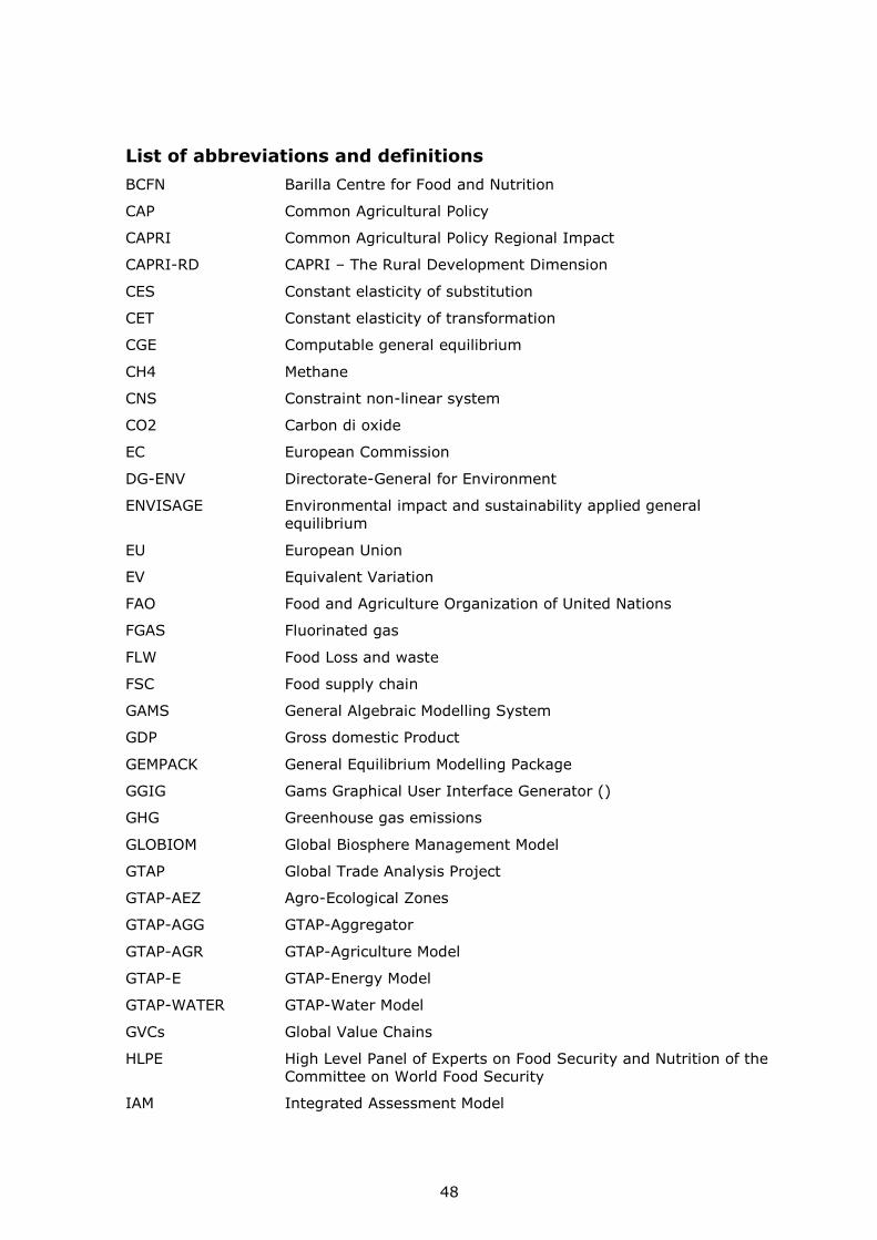
48

List of abbreviations and definitions

BCFN Barilla Centre for Food and Nutrition

CAP Common Agricultural Policy

CAPRI Common Agricultural Policy Regional Impact

CAPRI-RD CAPRI – The Rural Development Dimension

CES Constant elasticity of substitution

CET Constant elasticity of transformation

CGE Computable general equilibrium

CH4 Methane

CNS Constraint non-linear system

CO2 Carbon di oxide

EC European Commission

DG-ENV Directorate-General for Environment

ENVISAGE Environmental impact and sustainability applied general

equilibrium

EU European Union

EV Equivalent Variation

FAO Food and Agriculture Organization of United Nations

FGAS Fluorinated gas

FLW Food Loss and waste

FSC Food supply chain

GAMS General Algebraic Modelling System

GDP Gross domestic Product

GEMPACK General Equilibrium Modelling Package

GGIG Gams Graphical User Interface Generator ()

GHG Greenhouse gas emissions

GLOBIOM Global Biosphere Management Model

GTAP Global Trade Analysis Project

GTAP-AEZ Agro-Ecological Zones

GTAP-AGG GTAP-Aggregator

GTAP-AGR GTAP-Agriculture Model

GTAP-E GTAP-Energy Model

GTAP-WATER GTAP-Water Model

GVCs Global Value Chains

HLPE High Level Panel of Experts on Food Security and Nutrition of the

Committee on World Food Security

IAM Integrated Assessment Model

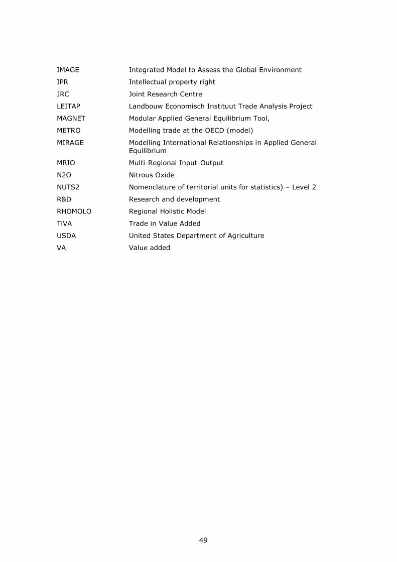
49

IMAGE Integrated Model to Assess the Global Environment

IPR Intellectual property right

JRC Joint Research Centre

LEITAP Landbouw Economisch Instituut Trade Analysis Project

MAGNET Modular Applied General Equilibrium Tool,

METRO Modelling trade at the OECD (model)

MIRAGE Modelling International Relationships in Applied General

Equilibrium

MRIO Multi-Regional Input-Output

N2O Nitrous Oxide

NUTS2 Nomenclature of territorial units for statistics) – Level 2

R&D Research and development

RHOMOLO Regional Holistic Model

TiVA Trade in Value Added

USDA United States Department of Agriculture

VA Value added

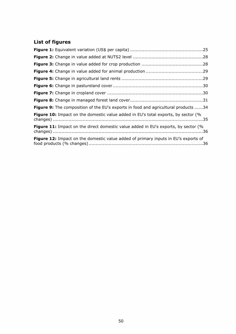
50

List of figures

Figure 1: Equivalent variation (US$ per capita) ...................................................25

Figure 2: Change in value added at NUTS2 level .................................................28

Figure 3: Change in value added for crop production ...........................................28

Figure 4: Change in value added for animal production ........................................29

Figure 5: Change in agricultural land rents .........................................................29

Figure 6: Change in pastureland cover ...............................................................30

Figure 7: Change in cropland cover ...................................................................30

Figure 8: Change in managed forest land cover ...................................................31

Figure 9: The composition of the EU's exports in food and agricultural products ......34

Figure 10: Impact on the domestic value added in EU's total exports, by sector (%

changes) .........................................................................................................35

Figure 11: Impact on the direct domestic value added in EU's exports, by sector (%

changes) .........................................................................................................36

Figure 12: Impact on the domestic value added of primary inputs in EU’s exports of

food products (% changes) ................................................................................36

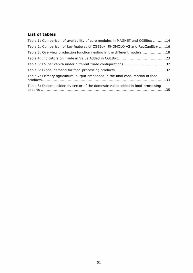
51

List of tables

Table 1: Comparison of availability of core modules in MAGNET and CGEBox ...........14

Table 2: Comparison of key features of CGEBox, RHOMOLO V2 and RegCgeEU+ ......16

Table 3: Overview production function nesting in the different models ....................18

Table 4: Indicators on Trade in Value Added in CGEBox .........................................23

Table 5: EV per capita under different trade configurations ....................................32

Table 6: Global demand for food-processing products ...........................................32

Table 7: Primary agricultural output embedded in the final consumption of food

products ..........................................................................................................33

Table 8: Decomposition by sector of the domestic value added in food-processing

exports ...........................................................................................................35

52

Annexes

Annex 1. Implementation of the TiVA indicators

Import shares

In the standard GTAP model, the Armington agents share the lower nest which splits

up total import demand to the different origins. The TiVA matrix to invert hence needs

to use these shares to convert the total import demand of an activity a for a

commodity i into bi-lateral import demand.

In first step, we calculate bi-lateral import shares based on CIF prices plus import

taxes, by first assigning the value (quantity times price)

*

* --- import shares, reconverted into fob

*

$$iftheni.MRIO "%modulesGTAP_MRIO%"=="on"

p_impShares(rsNat,rsNat1,iIn(i),%arg1%) $ pmCif.l(rsNat1,i,rsNat,%arg2%)

= p_results(rsNat,"Q",i,rsNat1,"int",%arg1%,"%version%")

* (pmCif.l(rsNat1,i,rsNat,%arg2%)*(1+imptx(rsNat1,i,rsNat,%arg2%)));

$$else.MRIO

p_impShares(rsNat,rsNat1,iIn(i),%arg1%) $ pmCif.l(rsNat1,i,rsNat,%arg2%)

= p_results(rsNat,"Q",i,rsNat1,"imp",%arg1%,"%version%")

* (pmCif.l(rsNat1,i,rsNat,%arg2%)*(1+imptx(rsNat1,i,rsNat,%arg2%)));

$$endif.MRIO

And next converting into shares by calculating the total and dividing by it:

*

* --- scale imports to unity by calcuation of total and division by total

*

p_impShares(rsNat,"wor",iIn(i),%arg1%) =

sum(rsNat1,p_impShares(rsNat,rsNat1,i,%arg1%));

p_impShares(rsNat,rsNat1,iIn(i),%arg1%) $ p_impShares(rsNat,rsNat1,i,%arg1%)

=

p_impShares(rsNat,rsNat1,i,%arg1%)/p_impShares(rsNat,"wor",i,%arg1%);

Trade margin demand

We next set back to f.o.b. basis:

p_impShares(rsNat,rsNat1,iIn(i),%arg1%) $ p_impShares(rsNat,rsNat1,i,%arg1%)

= p_impShares(rsNat,rsNat1,i,%arg1%)

/((pmCif.l(rsNat1,i,rsNat,%arg2%)*(1+imptx(rsNat1,i,rsNat,%arg2%)));

That re-definition is necessary to reflect that trade margins in GTAP are defined

relative to f.o.b. and request also composite input demand. We hence first calculate

the physical total (implicit) trade margin demand for margin products m for the

production activity a in regions rsNat:

*

* --- assign output used for trade margins to IO coefficients

*

p_trdMrg(rsNat,"tot",m,a,%arg1%)

*

* --- imports from rsNat1 of all products

*

= sum(((rsNat1,i) $ p_impShares(rsNat,rsNat1,i,%arg1%),

*

* --- total imports times times shares

*

p_results(rsNat,"Q",i,a,"imp",%arg1%,"%version%") *

p_impShares(rsNat,rsNat1,i,%arg1%)

*

* --- global margin demand

*

* tmarg(rsNat1,i,rsNat,%arg2%) * amgm(m,rsNat1,i,rsNat));

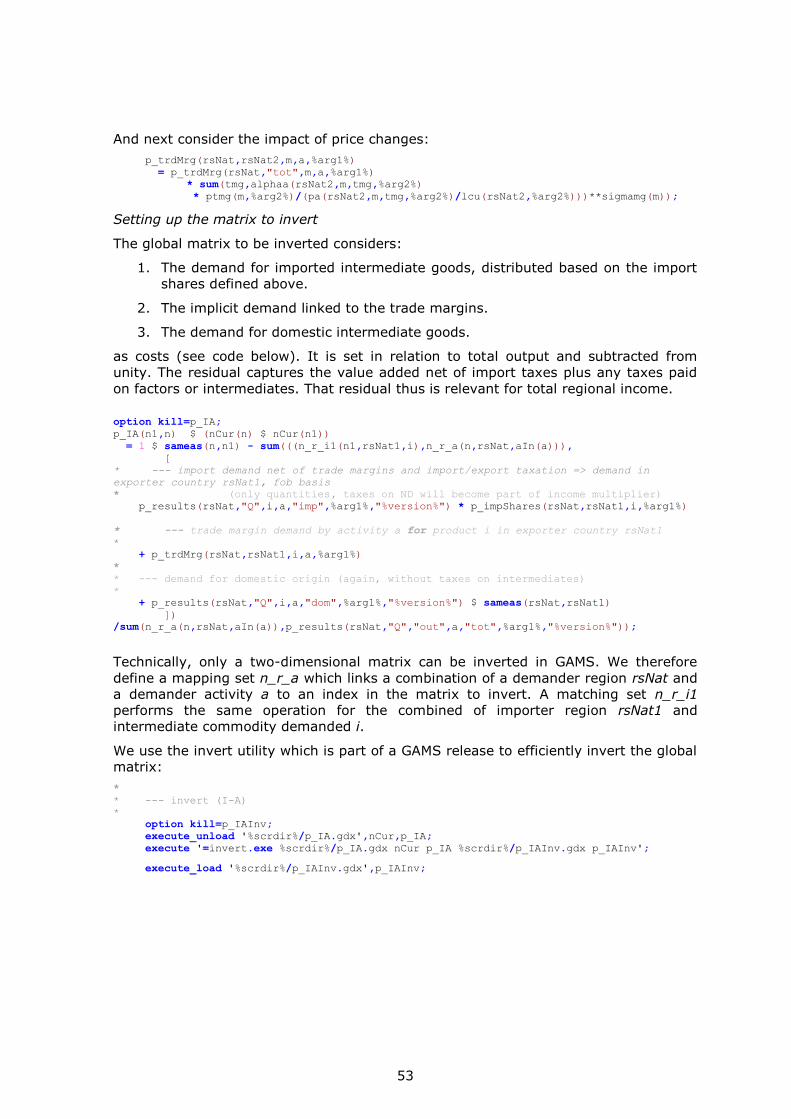
53

And next consider the impact of price changes:

p_trdMrg(rsNat,rsNat2,m,a,%arg1%)

= p_trdMrg(rsNat,"tot",m,a,%arg1%)

* sum(tmg,alphaa(rsNat2,m,tmg,%arg2%)

* ptmg(m,%arg2%)/(pa(rsNat2,m,tmg,%arg2%)/lcu(rsNat2,%arg2%)))**sigmamg(m));

Setting up the matrix to invert

The global matrix to be inverted considers:

1. The demand for imported intermediate goods, distributed based on the import

shares defined above.

2. The implicit demand linked to the trade margins.

3. The demand for domestic intermediate goods.

as costs (see code below). It is set in relation to total output and subtracted from

unity. The residual captures the value added net of import taxes plus any taxes paid

on factors or intermediates. That residual thus is relevant for total regional income.

option kill=p_IA;

p_IA(n1,n) $ (nCur(n) $ nCur(n1))

= 1 $ sameas(n,n1) - sum(((n_r_i1(n1,rsNat1,i),n_r_a(n,rsNat,aIn(a))),

[

* --- import demand net of trade margins and import/export taxation => demand in

exporter country rsNat1, fob basis

* (only quantities, taxes on ND will become part of income multiplier)

p_results(rsNat,"Q",i,a,"imp",%arg1%,"%version%") * p_impShares(rsNat,rsNat1,i,%arg1%)

* --- trade margin demand by activity a for product i in exporter country rsNat1

*

+ p_trdMrg(rsNat,rsNat1,i,a,%arg1%)

*

* --- demand for domestic origin (again, without taxes on intermediates)

*

+ p_results(rsNat,"Q",i,a,"dom",%arg1%,"%version%") $ sameas(rsNat,rsNat1)

])

/sum(n_r_a(n,rsNat,aIn(a)),p_results(rsNat,"Q","out",a,"tot",%arg1%,"%version%"));

Technically, only a two-dimensional matrix can be inverted in GAMS. We therefore

define a mapping set n_r_a which links a combination of a demander region rsNat and

a demander activity a to an index in the matrix to invert. A matching set n_r_i1

performs the same operation for the combined of importer region rsNat1 and

intermediate commodity demanded i.

We use the invert utility which is part of a GAMS release to efficiently invert the global

matrix:

*

* --- invert (I-A)

*

option kill=p_IAInv;

execute_unload '%scrdir%/p_IA.gdx',nCur,p_IA;

execute '=invert.exe %scrdir%/p_IA.gdx nCur p_IA %scrdir%/p_IAInv.gdx p_IAInv';

execute_load '%scrdir%/p_IAInv.gdx',p_IAInv;

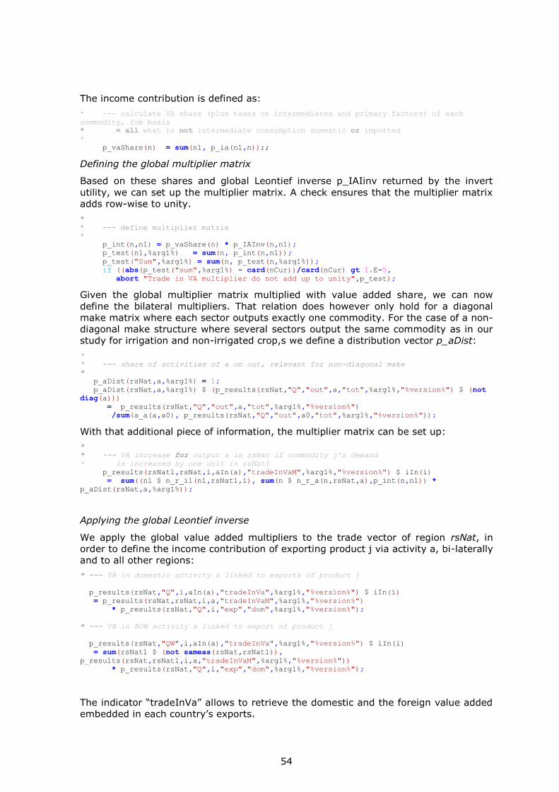
54

The income contribution is defined as:

* --- calculate VA share (plus taxes on intermediates and primary factors) of each

commodity, fob basis

* = all what is not intermediate consumption domestic or imported

*

p_vaShare(n) = sum(n1, p_ia(n1,n));;

Defining the global multiplier matrix

Based on these shares and global Leontief inverse p_IAIinv returned by the invert

utility, we can set up the multiplier matrix. A check ensures that the multiplier matrix

adds row-wise to unity.

*

* --- define multiplier matrix

*

p_int(n,n1) = p_vaShare(n) * p_IAInv(n,n1);

p_test(n1,%arg1%) = sum(n, p_int(n,n1));

p_test("Sum",%arg1%) = sum(n, p_test(n,%arg1%));

if ((abs(p_test("sum",%arg1%) - card(nCur))/card(nCur) gt 1.E-5,

abort "Trade in VA multiplier do not add up to unity",p_test);

Given the global multiplier matrix multiplied with value added share, we can now

define the bilateral multipliers. That relation does however only hold for a diagonal

make matrix where each sector outputs exactly one commodity. For the case of a non-

diagonal make structure where several sectors output the same commodity as in our

study for irrigation and non-irrigated crop,s we define a distribution vector p_aDist:

*

* --- share of activities of a on out, relevant for non-diagonal make

*

p_aDist(rsNat,a,%arg1%) = 1;

p_aDist(rsNat,a,%arg1%) $ (p_results(rsNat,"Q","out",a,"tot",%arg1%,"%version%") $ (not

diag(a)))

= p_results(rsNat,"Q","out",a,"tot",%arg1%,"%version%")

/sum(a_a(a,a0), p_results(rsNat,"Q","out",a0,"tot",%arg1%,"%version%"));

With that additional piece of information, the multiplier matrix can be set up:

*

* --- VA increase for output a in rsNat if commodity j's demand

* is increased by one unit in rsNat1

p_results(rsNat1,rsNat,i,aIn(a),"tradeInVaM",%arg1%,"%version%") $ iIn(i)

= sum((n1 $ n_r_i1(n1,rsNat1,i), sum(n $ n_r_a(n,rsNat,a),p_int(n,n1)) *

p_aDist(rsNat,a,%arg1%));

Applying the global Leontief inverse

We apply the global value added multipliers to the trade vector of region rsNat, in

order to define the income contribution of exporting product j via activity a, bi-laterally

and to all other regions:

* --- VA in domestic activity a linked to exports of product j

p_results(rsNat,"Q",i,aIn(a),"tradeInVa",%arg1%,"%version%") $ iIn(i)

= p_results(rsNat,rsNat,i,a,"tradeInVaM",%arg1%,"%version%")

* p_results(rsNat,"Q",i,"exp","dom",%arg1%,"%version%");

* --- VA in ROW activity a linked to export of product j

p_results(rsNat,"QW",i,aIn(a),"tradeInVa",%arg1%,"%version%") $ iIn(i)

= sum(rsNat1 $ (not sameas(rsNat,rsNat1)),

p_results(rsNat,rsNat1,i,a,"tradeInVaM",%arg1%,"%version%"))

* p_results(rsNat,"Q",i,"exp","dom",%arg1%,"%version%");

The indicator “tradeInVa” allows to retrieve the domestic and the foreign value added

embedded in each country’s exports.

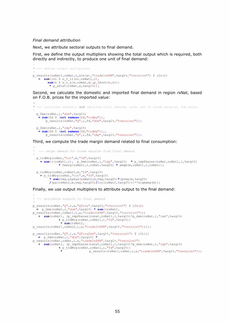
55

Final demand attribution

Next, we attribute sectoral outputs to final demand.

First, we define the output multipliers showing the total output which is required, both

directly and indirectly, to produce one unit of final demand:

*

* --- define output multipliers

*

p_results(rsNat1,rsNat,i,aIn(a),"tradeInXPM",%arg1%,"%version%") $ iIn(i)

= sum((n1 $ n_r_i1(n1,rsNat1,i),

sum(n $ n_r_a(n,rsNat,a),p_IAInv(n,n1))

* p_aDist(rsNat,a,%arg1%));

Second, we calculate the domestic and imported final demand in region rsNat, based

on F.O.B. prices for the imported value:

*

* --- calculate domestic and imported final demand, later net of trade margins, fob basis

*

p_Dem(rsNat,i,"dom",%arg1%)

= sum(fd $ (not sameas(fd,"trdmg")),

p_results(rsNat,"Q",i,fd,"dom",%arg1%,"%version%"));

p_Dem(rsNat,i,"imp",%arg1%)

= sum(fd $ (not sameas(fd,"trdmg")),,

p_results(rsNat,"Q",i,fd,"imp",%arg1%,"%version%"));

Third, we compute the trade margin demand related to final consumption:

*

* --- asign demand for trade margins from final demand

*

p_trdMrg(rsNat,"tot",m,"fd",%arg1%)

= sum(((rsNat1,i), p_Dem(rsNat,i,"imp",%arg1%) * p_impShares(rsNat,rsNat1,i,%arg1%)

* tmarg(rsNat1,i,rsNat,%arg2%) * amgm(m,rsNat1,i,rsNat));

p_trdMrg(rsNat,rsNat2,m,"fd",%arg1%)

= p_trdMrg(rsNat,"tot",m,"fd",%arg1%)

* sum(tmg,alphaa(rsNat2,m,tmg,%arg2%)*(ptmg(m,%arg2%)

/(pa(rsNat2,m,tmg,%arg2%)/lcu(rsNat2,%arg2%)))**sigmamg(m));

Finally, we use output multipliers to attribute output to the final demand:

*

* --- attribute outputs to final demand

*

p_results(rsNat,"Q",i,a,"QTiva",%arg1%,"%version%") $ iIn(i)

= p_Dem(rsNat,i,"dom",%arg1%) * sum((rsNat1,

p_results(rsNat,rsNat1,i,a,"tradeInXPM",%arg1%,"%version%")))

+ sum(rsNat1, (p_impShares(rsnat,rsNat1,i,%arg1%)*p_dem(rsNat,i,"imp",%arg1%)

+ p_trdMrg(rsNat,rsNat1,i,"fd",%arg1%))

* sum(rsNat2,

p_results(rsNat1,rsNat2,i,a,"tradeInXPM",%arg1%,"%version%"))));

p_results(rsNat,"Q",i,a,"QTivaDom",%arg1%,"%version%") $ iIn(i)

= p_Dem(rsNat,i,"dom",%arg1%) *

p_results(rsNat,rsNat,i,a,"tradeInXPM",%arg1%,"%version%")

+ sum(rsNat1, (p_impShares(rsnat,rsNat1,i,%arg1%)*p_dem(rsNat,i,"imp",%arg1%)

+ p_trdMrg(rsNat,rsNat1,i,"fd",%arg1%))

* p_results(rsNat1,rsNat,i,a,"tradeInXPM",%arg1%,"%version%"));

GETTING IN TOUCH WITH THE EU

In person

All over the European Union there are hundreds of Europe Direct information centres. You can find the address of the centre nearest you at: http://europea.eu/contact

On the phone or by email

Europe Direct is a service that answers your questions about the European Union. You can contact this service:

- by freephone: 00 800 6 7 8 9 10 11 (certain operators may charge for these calls),

- at the following standard number: +32 22999696, or

- by electronic mail via: http://europa.eu/contact

FINDING INFORMATION ABOUT THE EU

Online

Information about the European Union in all the official languages of the EU is available on the Europa website at: http://europa.eu

EU publications You can download or order free and priced EU publications from EU Bookshop at:

http://bookshop.europa.eu. Multiple copies of free publications may be obtained by contacting Europe

Direct or your local information centre (see http://europa.eu/contact).

KJ-N

A-2

9434-E

N-N

doi:10.2760/942172

ISBN 978-92-79-97246-1