ECONOMY & ENVIRONMENTdocuments.worldbank.org/curated/en/677081531112268818/...i Santiago Enriquez...
63
I Santiago Enriquez Bjorn Larsen Ernesto Sánchez-Triana GOOD PRACTICE NOTE 8 Local Environmental Externalities due to Energy Price Subsidies: A Focus on Air Pollution and Health ECONOMY & ENVIRONMENT Public Disclosure Authorized Public Disclosure Authorized Public Disclosure Authorized Public Disclosure Authorized
Transcript of ECONOMY & ENVIRONMENTdocuments.worldbank.org/curated/en/677081531112268818/...i Santiago Enriquez...

i
Santiago Enriquez
Bjorn Larsen
Ernesto Sánchez-Triana
GOOD PRACTICE NOTE 8Local Environmental Externalities due to Energy Price Subsidies: A Focus on Air Pollution and Health
ECONOMY & ENVIRONMENT
Pub
lic D
iscl
osur
e A
utho
rized
Pub
lic D
iscl
osur
e A
utho
rized
Pub
lic D
iscl
osur
e A
utho
rized
Pub
lic D
iscl
osur
e A
utho
rized

i i
GOOD PRACTiCE NOTE 8: LOCAL ENViRONMENTAL EXTERNALiTiES DUE TO ENERGY PRiCE SUBSiDiES
CONTENTS
Acknowledgments v
About the Authors v
Acronyms and Abbreviations vi
Summary 1
1. Introduction 4
2. Methodological Approach to Assessing Local Externalities of Energy Subsidies 8
3. Prioritizing the Analysis 11
Fossil Fuel Consumption Patterns 11
Emissions 11
A Fuel and Technology Perspective . . . . . . . . . . . . . . . . . . . . . . . . . . . . . . . . . . . . . . . 12
A Sector Perspective . . . . . . . . . . . . . . . . . . . . . . . . . . . . . . . . . . . . . . . . . . . . . . . . . . 14
Population Exposure 15
Dispersion of Emissions . . . . . . . . . . . . . . . . . . . . . . . . . . . . . . . . . . . . . . . . . . . . . . . . 16
Exposure . . . . . . . . . . . . . . . . . . . . . . . . . . . . . . . . . . . . . . . . . . . . . . . . . . . . . . . . . . . 18
4. Energy Consumption Effects of Price Subsidies 19
Choice of Analytical Model 20
Price Elasticities of Energy Demand 21
Substitution among Energy Sources 22
5. Higher Air Emissions from Energy Price Subsidies 24
Motorized Road Transport 24
Residential Sector 26
industry 27
Electricity 27
6. Population Exposure Assessment 28
Dispersion Modeling 28
intake Fractions 29
intake Fraction Applications 31

i i i
Proposed Approach 32
Distributed Ground-Level Emissions . . . . . . . . . . . . . . . . . . . . . . . . . . . . . . . . . . . . . 32
Power Plant Emissions . . . . . . . . . . . . . . . . . . . . . . . . . . . . . . . . . . . . . . . . . . . . . . . . 32
Industry . . . . . . . . . . . . . . . . . . . . . . . . . . . . . . . . . . . . . . . . . . . . . . . . . . . . . . . . . . . 32
Baseline Outdoor PM2.5 Concentrations . . . . . . . . . . . . . . . . . . . . . . . . . . . . . . . . . . . 32
7. Health Effects 34
Outdoor Air Pollution 34
Mortality . . . . . . . . . . . . . . . . . . . . . . . . . . . . . . . . . . . . . . . . . . . . . . . . . . . . . . . . . . 34
Morbidity . . . . . . . . . . . . . . . . . . . . . . . . . . . . . . . . . . . . . . . . . . . . . . . . . . . . . . . . . . 35
Household Air Pollution 36
Mortality . . . . . . . . . . . . . . . . . . . . . . . . . . . . . . . . . . . . . . . . . . . . . . . . . . . . . . . . . . 36
Morbidity . . . . . . . . . . . . . . . . . . . . . . . . . . . . . . . . . . . . . . . . . . . . . . . . . . . . . . . . . . 37
8. The Value of Health Effects 38
Mortality 38
Morbidity 38
Using the Value of Health Effects to inform Policy Options 39
9. Air Pollution Health Risk Assessment Tools 40
10. Conclusions 42
Annex 1: Emission Intake Fractions 43
Annex 2: Methodology for Estimating Health Effects 44
Annex 3: Valuing the Health Effects of Energy Subsidies 46
References 48
Endnotes 54

iV
GOOD PRACTiCE NOTE 8: LOCAL ENViRONMENTAL EXTERNALiTiES DUE TO ENERGY PRiCE SUBSiDiES
TABLES
Table 1: Quantifying the Effects of Energy Price Subsidies on Local Air Pollution and Health 10
Table 2: Energy Consumption Effects of Energy Price Subsidies 20
Table 3: Average Price Elasticities of Energy Demand 21
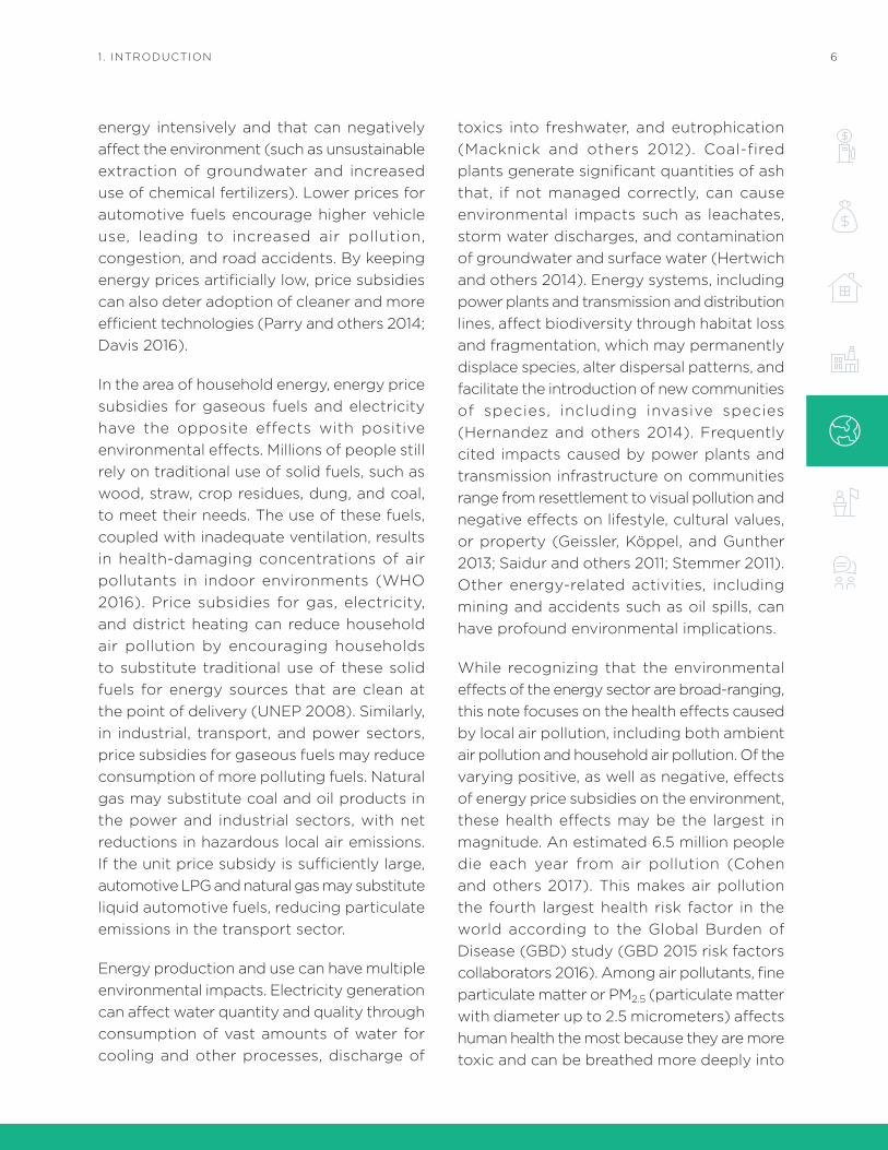
Table 4: Examples of Substitution among Energy Sources by Sector 23
Table 5: European Union Light-Duty Diesel Vehicle Emission Standards for PM 25
Table 6: European Union Heavy-Duty Diesel Engines Emission Standards for PM 25
Table 7: Population Weighted Mean intra-Urban intake Fractions of Distributed Ground-Level Emissions 29
Table 8: Summary of Recommended intake Fractions 30
Table 9: Recommended PM2.5 intake Fractions by Region 30
Table 10: intake Fraction Estimates across 29 Power Plant Sites throughout China 31
Table 11: Premature Deaths and Days of illness Caused Annually by Household Air Pollution and Their Associated Costs in Selected Jurisdictions 39
Table 12: Key Characteristics of Air Pollution Health Risk Assessment tools 41
FiGURES
Figure 1: National and Subnational Level Comparisons—Cost of Environmental Health Effects Caused by Air Pollution 7
Figure 2: Estimated Annual Average PM2.5 33
Figure 3: Relative Risks of Major Health Outcomes Associated with PM2.5 Exposure 35
BOXES
Box 1: Using income and Price Elasticity to Estimate Gasoline Consumption Reduction from Price Subsidy Removal in Mexico 22

V
ACKNOWLEDGMENTS
ACKNOWLEDGMENTS
This is the eighth in the series of 10 good practice notes under the Energy Sector Reform Assessment Framework (ESRAF), an initiative of the Energy Sector Management Assistance Program (ESMAP) of the World Bank. ESRAF proposes a guide to analyzing energy subsidies, the impacts of subsidies and their reforms, and the political context for reform in developing countries.
The authors would like to acknowledge the contributions of Dan Biller and Giovanni Ruta, who peer reviewed this good practice note. The authors are thankful to Thomas Flochel, Marianne Fey, and Masami Kojima for their guidance, support, and review of the good practice note.
ABOUT THE AUTHORS
Santiago Enriquez is an international consultant with more than 18 years of experience in the design, implementation, and evaluation of policies relating to the environment, conservation, and climate change. He has developed analytical work for the World Bank, the United States Agency for international Development, and the inter-American Development Bank on topics that include mainstreaming of environmental and climate change considerations in key economic sectors, institutional and organizational analyses to strengthen environmental management, and policy-based strategic environmental assessments. From 1998 to 2002, he worked at the international Affairs Unit of Mexico’s Ministry of Environment and Natural Resources. He holds a master’s degree in public policy from the Harvard Kennedy School.
Bjorn Larsen is an international development economist and consultant to international and bilateral development agencies, consulting firms, and research institutions with more than 25 years of professional experience. His primary fields of consulting and research are environmental health and natural resource management from over 50 countries in Asia, Central and South America, Europe, Middle East and North Africa, and Sub-Saharan Africa. Fields of expertise include environmental health risk assessment, health valuation, cost-benefit analysis, poverty-environment linkages, child malnutrition and environment linkages, natural resource degradation and valuation, poverty and natural resources, household survey design and administration, and statistical analysis of household survey data. He has worked extensively on indoor air pollution from solid fuels, urban air pollution, water supply, sanitation and hygiene, and child nutrition and health.

Vi
GOOD PRACTiCE NOTE 8: LOCAL ENViRONMENTAL EXTERNALiTiES DUE TO ENERGY PRiCE SUBSiDiES
Ernesto Sánchez-Triana is the global lead for environmental health and pollution management for the World Bank. He has worked on projects in numerous countries, including Afghanistan, Argentina, Bangladesh, Bhutan, Bolivia, Brazil, Cambodia, Ecuador, india, the Lao People’s Democratic Republic, Mexico, Pakistan, Panama, Paraguay, and Peru. Before joining the World Bank, he worked for the inter-American Development Bank. He has led the preparation of numerous policy-based programs, investment projects, technical assistance operations, and analytical works. He holds two master’s degrees and a Ph.D. from Stanford University. He has authored numerous publications on pollution management, clean production, environmental economics, energy efficiency, environmental policy, organizational learning, poverty assessment, and green growth.
ACRONYMS AND ABBREViATiONS
ALRI acute lower respiratory infection
ARB California Air Resources Board
CATEF California Air Toxics Emission Factor
CMB chemical mass balance
CNG compressed natural gas
COPD chronic obstructive pulmonary disease
CP cardiopulmonary (mortality)
DALYs disability-adjusted life-years
EMFAC EMission FACtors
EPA U.S. Environmental Protection Agency
ESRAF Energy Sector Reform Assessment Framework
ESMAP Energy Sector Management Assistance Program
g gram
GBD Global Burden of Disease
GDP gross domestic product
HAPIT Household Air Pollution impacts
IHD ischemic heart disease
km kilometer

Vii
ACRONYMS AND ABBREViATiONS
kW kilowatt
kWh kilowatt-hour
LCIA life cycle impact assessment
LCV light commercial vehicle
LPG liquefied petroleum gas
µg microgram
m3 cubic meter
NH3 ammonia
NOx oxide of nitrogen
N2O oxide of sulfur
OECD Organisation for Economic Co-operation and Development
PAF population attributable fraction
PIF potential impact fraction
PM2.5 particulate matter with a diameter of less than 2.5 microns
PM10 particulate matter with a diameter of less than 10 microns
ppm parts per million
PPP purchasing power parity
RR relative risk
SBP systolic blood pressure
SOx oxides of sulfur
UNEP United Nations Environment Programme
VSL value of statistical life
WHO World Health Organization
WTP willingness to pay
YLD years of life lost to disability

1 GOOD PRACTICE NOTE 8: LOCAL ENVIRONMENTAL EXTERNALITIES DUE TO ENERGY PRICE SUBSIDIES
SUMMARY
This note aims to provide an overview and guidance on the use of tools to assess the environmental and health effects of changes in the levels of fine particulate matter caused by higher consumption of energy due to subsidized prices at the country level. it also provides information to help practitioners develop reliable estimates even in the absence of data and with limited resources.
The topic of the note is highly complex and involves multiple fields and disciplines. The note attempts to reduce such complexity by breaking the assessment down into several distinct steps, each with its own methodologies. The note is intended to serve as a source of resources and practical advice to guide practitioners along each of these steps.
Higher consumption of energy arising from energy subsidies that keep consumer prices artificially low can have adverse local and global environmental impacts. An increase in energy consumption can increase local air pollution, global greenhouse gas emissions, water pollution, and soil contamination from energy production and use. Energy production and use are a significant source of global emissions of fine particulate matter, as well as oxides of nitrogen and sulfur, both precursors to fine particulate matter. Price subsidies for energy can also lead to an increase in energy-intensive activities and products that can negatively affect the environment (such as unsustainable extraction of groundwater and increased use of chemical fertilizers).
However, energy price subsidies can also have positive environmental effects. Millions of people still rely on solid biomass and coal
to meet their needs. Traditional use of these solid fuels (that is, not burning them in stoves with high combustion efficiency), coupled with inadequate ventilation, results in health-damaging concentrations of air pollutants in indoor environments. Price subsidies for gas and electricity can reduce household air pollution by encouraging households to substitute traditional energy sources with cleaner forms of energy. Price subsidies for natural gas can also reduce coal and oil product consumption in the power and industrial sectors, with net reductions in hazardous local air emissions. Similarly, lower prices of automotive LPG and natural gas due to subsidies can reduce particulate emissions when these fuels are substitutes for liquid automotive fuels.
Consumer price subsidies for energy have indirect effects on pollution, which might be either positive or negative, depending on a number of factors, including the energy sources and the uses they target. Therefore, an understanding of the linkages among energy price subsidies, environmental quality, and health can inform energy subsidy reforms and identify measures to mitigate the potential negative environmental impacts of subsidy removal.
While recognizing that the environmental effects of the energy sector are broad-ranging, this note focuses on local air pollution and health because it is arguably the energy-related local environmental externality with the largest social cost globally. An estimated 6.5 million people died from outdoor ambient and household air pollution in 2015 (Cohen and others 2017). Household air pollution

2SUMMARY
also contributes to outdoor ambient air pollution, because pollutants are not confined strictly to rooms where solid fuels are burned for cooking and heating. Several analyses conducted by the World Bank found that ambient air pollution had an average cost of 3.5% of gross domestic product (GDP) in five Asian countries and 2.5% of GDP in six Latin American countries. Household air pollution had a cost that was as high as 3.3% of GDP in Apurimac, Peru, and 4.9% of GDP in the Lao People’s Democratic Republic. Higher prices for polluting fuels can help reduce their consumption, thereby potentially helping to reduce air pollution; conversely higher prices for cleaner fuels could aggravate air pollution.
While price subsidies to coal have declined substantially since the 1990s, those to oil products and natural gas remain in a number of countries. Electricity tariff subsidies are also prevalent in many countries. Such subsidies can contribute to overconsumption of energy. Where energy is derived from fossil fuels, overconsumption leads to higher air pollution.
This note proposes a five-step analysis to assess the health effects of energy price subsidies, focusing on
1 | The effect of consumer price subsidies on levels and patterns of energy consumption (section 4 of this note)
2 | Air emissions from energy consumption (section 5)
3 | Human exposure to air emissions (section 6)
4 | Health effects of exposure (section 7)
5 | Monetary valuation of health effects (section 8)
The note is confined to cases where there are no serious shortages of subsidized energy. Such shortages are pervasive in some countries and regions, such as in the power sector in Sub-Saharan Africa (Kojima and Trimble 2016). Where shortages are widespread—so that consumers are forced to go without the specific energy source or else pay much higher prices than the official ones—the methodologies outlined in this note are not applicable.
Defining the priority sector and fuels is crucial to conduct a useful assessment, given that it will likely be carried out with limited resources and data. in most countries, the adverse health effects of air pollution from energy price subsidies are caused by a few fuels and sectors. identifying these fuels and sectors can therefore be a useful first step (section 3). Based on current global energy subsidy patterns, the priority sectors for most countries from the point of view of public health will likely be industry, heat and power generation, residential, and road transportation.
Recent meta-analyses of price elasticities of energy demand by type of fuel and energy provide a basis for assessing the effect of price subsidies on energy consumption, provided subsidized energy is readily available to all consumers who wish to purchase it. Cross-price elasticities may be applied in sectors and to fuels where significant fuel substitution is likely. Using country-specific urban-transport-environment models would be advantageous, if available, because of the complexity of air emissions from motor vehicles.
This note focuses the analysis of price subsidies on primary and secondary fine particulate matter (PM2.5, atmospheric particulate matter with a diameter of less than 2.5 microns),

3 GOOD PRACTICE NOTE 8: LOCAL ENVIRONMENTAL EXTERNALITIES DUE TO ENERGY PRICE SUBSIDIES
the pollutant with the largest health effects worldwide, and using intake fractions to estimate population exposure to PM2.5 from fossil fuels and solid biomass. This approach is similar to that of recent global studies of energy price subsidies and taxes. The intake fractions are combined with the relative-risk functions for major health outcomes of air pollution from the Global Burden of Disease study to estimate the health effects associated with energy price subsidies.
The note proposes three geographic-demographic scales: urban areas with a population over 100,000, urban areas with a population less than 100,000, and rural areas. The note also discusses the availability of
monitoring measurement data and alternative options for determining ambient PM2.5 concentrations at the proposed geographic-demographic scale, as well as approaches to deal with data scarcity.
The proposed method for estimating the economic value of mortality caused by air pollution follows a recent World Bank report, using a cross-country transfer method of the value of statistical life (VSL). in addition, the note proposes methods for incorporating valuation of increased illness, although morbidity is generally found to constitute a relatively minor share of the health costs of air pollution.

41. iNTRODUCTiON
1. iNTRODUCTiON
This note provides an overview and guidance on the use of tools to assess the environmental and health effects of price subsidies for energy at the country level. it also provides information to help develop reliable estimates even in the absence of data and with limited resources. Assessing the environmental and health effects of energy price subsidies is highly complex and calls for an interdisciplinary approach. This note discusses available methodologies and provides examples where such an approach has been adopted, with the aim of sharing practical advice to practitioners interested in conducting similar assessments.
Good Practice Note 1 defines an energy subsidy as a deliberate policy action by the government that specifically targets electricity, fuels, or district heating and has one or more of the following effects:
• Reducing the net cost of energy purchased
• Reducing the cost of energy production or delivery
• increasing revenues retained by energy producers and suppliers
These include government control of energy prices that are kept artificially low; budgetary transfers to state-owned energy suppliers or tax expenditures granted to energy suppliers to keep costs down to benefit consumers, producers, or both; underpricing of goods and services provided to energy suppliers such as fuels, land, and water; subsidized loans; and shifting of risk burdens, such as assumption of risks through limits on commercial liability.
There are several mechanisms through which the subsidies as defined above can affect the local and global environment:
• Prices that are artificially low. This is the focus of this note and arguably the most frequently cited case, assumed to increase consumption relative to the counterfactual of no subsidies. Prices may be low because the government sets low prices or price ceilings, restricts exports of the energy in question, or provides producer support (tax expenditures, underpricing of access to land and other goods and services, below-market provision of loans) with the objective of lowering prices. Low prices for clean fuels may have positive effects on the environment, and conversely low prices for polluting fuels are likely to have negative effects. Subsidized fuel inputs to production sectors, including electricity generation and district heating, are also likely to increase consumption compared to the situation with no subsidized inputs. However, as Good Practice Note 1 details, unintended consequences of subsidies that lower the official prices dampen these effects.

5 GOOD PRACTICE NOTE 8: LOCAL ENVIRONMENTAL EXTERNALITIES DUE TO ENERGY PRICE SUBSIDIES
• Energy shortages. Low prices provide strong incentives for diversion of subsidized liquid fuels to ineligible beneficiaries, including out-smuggling. This has led to acute shortages in some countries, suppressing consumption. Price subsidies also discourage investment because investors fear that reimbursements may be late, inadequate, or both. Over time, the sector supplying the subsidized energy may decay if subsidized prices are below economic opportunity costs, let alone supply costs. This is one of the drivers of chronic power shortages in some countries, as well as fuel shortages in some major oil exporters that are having to import petroleum products at world prices because their refining sector is undercapitalized and in disrepair (such as in the islamic Republic of iran, iraq, and Nigeria). in the extreme, if higher unsubsidized prices eliminate fuel shortages, consumption may actually increase, rather than decrease, after subsidy removal (Kojima 2013; Kojima and Trimble 2016).
• Higher prices on the black market. Commercial malpractice in the form of illegal diversion and out-smuggling creates fuel shortages, which push up prices. There can be a large difference between official prices and prices actually paid. in estimating the impact of subsidy removal on consumption volume, it is important to use the actual prices paid, and not official prices, which can be considerably lower. in some cases, illegal diversion has been so widespread and rampant that consumers have ended up paying far more than even unsubsidized prices, as the example of subsidized kerosene in
Nigeria in box 6 of Good Practice Note 1 shows.
in assessing the impact of subsidized prices on consumption, it is critical to take into account both the actual prices paid and any limits on the availability of the subsidized energy. Many, if not most, studies examining the impact of subsidy removal do not take these two factors into account, leading to overestimation of the likely effect of subsidy removal.
On the other hand, refineries in disrepair are in no position to produce fuels meeting stringent specifications designed to protect public health. As a result, fuel quality may lag behind those in developed countries by years or even decades, preventing adoption of advanced exhaust control devices and even deactivating standard three-way catalytic converters in spark-ignition engines.
• Cash transfers to consumers. Energy prices may not be kept low, but if consumers are provided with conditional or unconditional cash transfers, consumption will be higher than otherwise. Cash transfers conditional upon energy purchase will increase consumption more than unconditional cash transfers, which the beneficiaries can use for any purpose. This form of subsidy is not considered in this note.
• Shifting of risk burden. Government assumption of environmental and safety risks, and consumer or resident assumption of risks through limits on commercial liability, may encourage energy producers to take undue risk at the cost of the environment, resulting in air and water pollution and soil contamination. This form of subsidy is not considered in this note.
Energy price subsidies can also lead to an increase in activities and products that use
61. iNTRODUCTiON
energy intensively and that can negatively affect the environment (such as unsustainable extraction of groundwater and increased use of chemical fertilizers). Lower prices for automotive fuels encourage higher vehicle use, leading to increased air pollution, congestion, and road accidents. By keeping energy prices artificially low, price subsidies can also deter adoption of cleaner and more efficient technologies (Parry and others 2014; Davis 2016).
in the area of household energy, energy price subsidies for gaseous fuels and electricity have the opposite effects with positive environmental effects. Millions of people still rely on traditional use of solid fuels, such as wood, straw, crop residues, dung, and coal, to meet their needs. The use of these fuels, coupled with inadequate ventilation, results in health-damaging concentrations of air pollutants in indoor environments (WHO 2016). Price subsidies for gas, electricity, and district heating can reduce household air pollution by encouraging households to substitute traditional use of these solid fuels for energy sources that are clean at the point of delivery (UNEP 2008). Similarly, in industrial, transport, and power sectors, price subsidies for gaseous fuels may reduce consumption of more polluting fuels. Natural gas may substitute coal and oil products in the power and industrial sectors, with net reductions in hazardous local air emissions. if the unit price subsidy is sufficiently large, automotive LPG and natural gas may substitute liquid automotive fuels, reducing particulate emissions in the transport sector.
Energy production and use can have multiple environmental impacts. Electricity generation can affect water quantity and quality through consumption of vast amounts of water for cooling and other processes, discharge of
toxics into freshwater, and eutrophication (Macknick and others 2012). Coal-fired plants generate significant quantities of ash that, if not managed correctly, can cause environmental impacts such as leachates, storm water discharges, and contamination of groundwater and surface water (Hertwich and others 2014). Energy systems, including power plants and transmission and distribution lines, affect biodiversity through habitat loss and fragmentation, which may permanently displace species, alter dispersal patterns, and facilitate the introduction of new communities of species, including invasive species (Hernandez and others 2014). Frequently cited impacts caused by power plants and transmission infrastructure on communities range from resettlement to visual pollution and negative effects on lifestyle, cultural values, or property (Geissler, Köppel, and Gunther 2013; Saidur and others 2011; Stemmer 2011). Other energy-related activities, including mining and accidents such as oil spills, can have profound environmental implications.
While recognizing that the environmental effects of the energy sector are broad-ranging, this note focuses on the health effects caused by local air pollution, including both ambient air pollution and household air pollution. Of the varying positive, as well as negative, effects of energy price subsidies on the environment, these health effects may be the largest in magnitude. An estimated 6.5 million people die each year from air pollution (Cohen and others 2017). This makes air pollution the fourth largest health risk factor in the world according to the Global Burden of Disease (GBD) study (GBD 2015 risk factors collaborators 2016). Among air pollutants, fine particulate matter or PM2.5 (particulate matter with diameter up to 2.5 micrometers) affects human health the most because they are more toxic and can be breathed more deeply into

7 GOOD PRACTICE NOTE 8: LOCAL ENVIRONMENTAL EXTERNALITIES DUE TO ENERGY PRICE SUBSIDIES
the lungs than other pollutants (Pope and Dockery 2006). incomplete combustion of fossil fuels and solid biomass is an important source of PM2.5 emissions and is responsible for a large share of these deaths (iEA 2016). Other sources of PM2.5 from fuel combustion include emissions of oxides of sulfur (SOx) and oxides of nitrogen (NOx), which form so-called secondary (sulfate-based and nitrate-based) particles through chemical reactions in the atmosphere. About 40% of the deaths are from household air pollution due to a lack of access to clean household energy, clean combustion technologies, or both, and 60% are caused by outdoor ambient air pollution.
Several analyses conducted by the World Bank found that the economic costs of the health effects caused by ambient and household air pollution are significant at the national and subnational levels. Per these studies, ambient air pollution had an average cost of 3.5% of gross domestic product (GDP) in five Asian countries and 2.5% of GDP in six Latin American countries. Household air pollution had a cost equivalent to 1% of GDP in many countries, and as high as 4.9% of GDP in the Lao People’s Democratic Republic. Figure 1
compares these estimates across selected national and subnational jurisdictions.
How much lower prices from subsidies increase the consumption of the subsidized energy, and the extent to which higher consumption in turn affects health are difficult to quantify because of a number of factors. An important point to stress is that emission characteristics of fuel combustion is a function of both the fuel properties and the technical state of the equipment burning the fuel. This is particularly true in the transport sector, where emission characteristics are a much greater function of the state of the vehicle than the fuel, especially in developing countries.
Frequently raised policy questions in the context of energy price subsidies and air pollution are who benefits most from the subsidies and who is affected by pollution. The first question is discussed in part in Good Practice Notes 3 and 4, both of which focus primarily on price subsidies captured by households. it is quite difficult to provide guidance to estimate the distributional impacts of outdoor air pollution within a whole country because the relevant variables vary widely from one location to another due to factors such as
FIGURE 1: National and Subnational Level Comparisons—Cost of Environmental Health Effects Caused by Air Pollution
0
1
2
3
4
5
6
Bolivia* Argentina* Peru* Lao PDR* Piauí, Brazil** Hidalgo,Mexico**
Apurimac,Peru**
Sindh,Pakistan**
% of GDP
Household Air Pollution
Outdoor Air Pollution
Note: * = National-level estimate; ** = Subnational-level estimate.
Sources: Larsen 2015, 2017a, 2017b; Larsen and Skjelvik 2013a, 2013b, 2014a, 2014b; Sánchez-Triana and others 2015.

82. METHODOLOGiCAL APPROACH TO ASSESSiNG LOCAL EXTERNALiTiES OF ENERGY SUBSiDiES
climate, topography, and urban development. This issue is therefore not addressed in this note. in the case of household air pollution, rural and poor households that cannot afford modern energy sources are primarily affected, although in some low-income and lower-middle-income countries, even the urban rich continue to cite solid fuels as their primary cooking fuels in household surveys. Women and infants face greater risks from indoor air pollution because they typically spend more time near the sources of household air pollution (Smith and others 2014).
This note is structured as follows. Section 2 explains the methodological approach to assess the local externalities of energy price subsidies. Section 3 provides guidance to prioritize the analysis, recognizing that scarce resources are generally available to conduct
this type of analysis and that most health effects associated with energy price subsidies are usually caused by a few fuels and in a small number of sectors. Section 4 focuses on the linkages between price subsidies and energy consumption, which are important to assess what portion of the negative externalities caused by air pollution can be reasonably associated with the existence of price subsidies. Section 5 discusses how energy consumption affects emissions of air pollutants. Section 6 focuses on different methods to estimate human exposure to such pollutants, while section 7 centers on the health effects resulting from said exposure. Section 8 describes methods to estimate the economic value of the health effects. Section 9 presents available automated air pollution health risk assessment tools. The note’s conclusions are presented in section 10.
2. METHODOLOGiCAL APPROACH TO ASSESSiNG LOCAL EXTERNALiTiES OF ENERGY SUBSiDiES
Estimating the health effects of local air pollution arising from energy price subsidies can be a complex task. Complex tasks often call for simplifications and approximations, both in terms of modeling and data application. Appreciating some of this complexity can help understand sources and magnitudes of uncertainty in health estimates associated with alternative methodological and data options. in addition, it is useful to differentiate between situations in which simplifications and approximations are acceptable and result in relatively small margins of error, and those in which the complexity warrants detailed assessment to provide meaningful estimates of health effects.
The complexity of estimating health effects of energy price subsidies can be characterized at five levels:
1 | The effect of price subsidies on levels and patterns of energy consumption (discussed in section 4 of this note)
2 | Air emissions from energy consumption (discussed in section 5)
3 | Human exposure to air emissions (discussed in section 6)
4 | Health effects of exposure (discussed in section 7)
5 | Monetary valuation of health effects (discussed in section 8)

9 GOOD PRACTICE NOTE 8: LOCAL ENVIRONMENTAL EXTERNALITIES DUE TO ENERGY PRICE SUBSIDIES
in the absence of information on vehicle stock characteristics, technologies of different combustion engines and boilers, the state of their maintenance and operations (including vehicle driving patterns), and other requisite data, vastly simplifying assumptions have to be made to quantify the impact on health of changes in fuel consumption. The relationship between fuel consumption and emissions may be highly nonlinear, as is the relationship between emissions and ambient concentrations. The nonlinear relationship between consumption and emissions is seldom, if ever, taken into account. The extent of simplification means that margins of error are certain to be large. Each step—estimation of pollutant emissions from fuel consumption, estimation of changes in the ambient concentrations of the pollutants from changes in fuel consumption, estimation of changes in health parameters in response to changes in ambient pollutant concentrations, and finally monetization of health damage—is complex, involving large assumptions.
An approach adopted by many is to ignore the foregoing factors affecting emissions, and simply assume a linear relationship between fuel consumption and emissions of pollutants. Such an assumption is valid for carbon dioxide (in the absence of carbon capture and storage), but not for PM2.5, the subject of this note, and other pollutants. Absent a very large-scale study, however, it would be difficult to take account of various factors affecting emissions of harmful pollutants, especially at the country level. if linearity is assumed at every step of the way, such a simplifying assumption leads to the following equation between a change in fuel consumption and its health effects in monetary terms (B):
B = ∆E * * V = ∆F * e * * V, (1)
where ΔE is change in air emissions (metric tons/year); ΔF is change in fuel consumption (metric tons/year), for the purpose of this note incremental fuel consumption that can be attributed to price subsidies; e is fuel emission factor (metric ton of pollutant emitted/metric ton of fuel consumed); δD/δE is health effects (for example, deaths per year) per metric ton of emissions; and V is the unit value of health effects. Because of nonlinearity, the accuracy of equation 1 increases with diminishing changes (that is, as the percentage changes in the parameters in the equation approach zero), and conversely the equation’s inaccuracy increases with increasing change. Where price subsidies are for electricity or district-heating tariffs, the change in electricity or heat consumption is first calculated, and these changes in turn need to be traced back to fuel consumption. This may not be straightforward. For example, for grid electricity, with a handful of exceptions (such as Liberia), it is almost certain that the power mix consists of several types of generation sources. How to calculate changes in fuel consumption in response to changes in electricity consumption is described in greater detail in section 4, subsection a.
To capture the total health effects of price subsidies, equation 1 would have to be estimated
1 | For all fuels directly and indirectly affected by the price subsidy to capture the effects of substitution among different energy sources;
2 | For each user of fuel within each sector, as fuel emission factors generally are user and sector specific;
3 | For each type of air emissions from fuel combustion;
δDδE
δDδE

102. METHODOLOGiCAL APPROACH TO ASSESSiNG LOCAL EXTERNALiTiES OF ENERGY SUBSiDiES
4 | For each type of health outcome affected by air emissions; and
5 | At small geographic scales, as health effects per metric ton of emissions vary geographically in relation to emission dispersion, ambient pollution concentrations, population density, and baseline health conditions.
Data constraints make the above level of detail even for this very limited equation practically impossible. Major data constraints generally include country- and sector-specific fuel emission factors. The dearth of local outdoor air pollution data is another
significant constraint, since on-the-ground monitoring data networks are largely missing or inadequately operated and maintained in most developing countries. Another source of uncertainty is the emissions for which health effects have not been rigorously established.
Each component of equation 1 is further discussed in the following sections to elaborate on the interactions among price subsidies, fuel consumption, emissions, health effects, and geographic scales. Table 1 provides an overview of the recommended steps to quantify the environmental health effects of energy price subsidies.
TABLE 1: Quantifying the Effects of Energy Price Subsidies on Local Air Pollution and Health
Steps Notes
1 Quantify energy price subsidies
• Focus on fossil fuels, electricity, and district heating.• Quantify the difference between unsubsidized prices and the actual prices paid by
consumers.• Calculate the unit price subsidy for each fuel in each sector, because price elasticities and
fuel emission factors vary across fuels and sectors.
2 Estimate the impact of price subsidies on energy consumption
Assess the extent of energy shortages. if serious, the procedure below could grossly overestimate energy consumption. if energy shortages are minor, then choose among the following tools:• Apply sector-specific own-price (and cross-price) elasticities of energy demand in partial
equilibrium if unit price subsidies are relatively “small”.• For electricity, investigate if there is a power sector model that can be used to estimate
which fuels are used more and by how much to meet the incremental power demand from lower electricity tariffs. Do the same for district heating if more than one fuel is used to generate heat.
• Apply sector models if price subsidies are concentrated in a few sectors and unit price subsidies are relatively large.
• Apply country-specific computable general equilibrium (CGE) models (if available) if subsidies prevail in most sectors and unit price subsidies are very large.
• Apply models for road transport sector or motor vehicle fleets if unit price subsidies for automotive fuels are relatively large, because of the complex nature of vehicle emissions.
3 Estimate impacts of energy consumption on emissions
• Focus on PM2.5 emissions.• Decide whether to include estimation of impacts on secondary PM2.5 (sulfates, nitrates).• Establish fuel- and sector-specific emission factors for fuels and sectors impacted by
price subsidies.• Estimate impacts on emissions in spatial aggregations according to population density,
exposure, and data availability.

11 GOOD PRACTICE NOTE 8: LOCAL ENVIRONMENTAL EXTERNALITIES DUE TO ENERGY PRICE SUBSIDIES
Steps Notes
4 Estimate health effects of changes in emissions
• Establish the prevailing outdoor PM2.5 concentrations in selected spatial aggregations (using available monitoring data or satellite/chemical transport model estimates).
• Choose whether to estimate health effects by using an “intake fraction” approach or by estimating the effect of changes in emissions on outdoor air quality.
• Apply generally accepted exposure-response functions (relative-risk functions) for estimating major health effects.
5 Estimate the monetary value of the health effects
• Establish a monetary value per unit of health effects, for example, the value of statistical life (VSL) for premature mortality.
• Multiply the unit monetary value by total health effects.
3. PRiORiTiZiNG THE ANALYSiS
in a majority of countries, the use of a few fuels in a limited number of sectors causes the most significant emissions of air pollutants and their impacts on health. Where energy price subsidies increase their consumption, or lead to greater use of polluting equipment, such subsidies exacerbate the adverse effects on health. Where the subsidies promote a shift away from polluting fuels to cleaner fuels, they can improve public health. identifying these fuels and sectors is a useful first step that can be carried out by mapping fossil fuel consumption patterns from national or subnational energy balances with subsidy levels, general patterns of emission intensities, and population exposure by sector.
FOSSIL FUEL CONSUMPTION PATTERNS
The power and heating sectors, including combined heat and power, together make up the largest consumer of fossil fuels, representing 34% of global fossil fuel consumption in 2015. Coal in 2015 accounted for 62% of all fossil fuels consumed in the sector (iEA 2017). The transport sector, which primarily uses diesel and gasoline, is the second largest consumer
of fossil fuels, followed by industry. LPG and natural gas use in the residential sector is important for improving public health because the only affordable substitutes tend to be highly polluting solid fuels with severe health effects of household air pollution.
EMISSIONS
As mentioned earlier, the air pollutant associated with the largest health effects at national and global scales is PM2.5. The Global Burden of Disease Study 2015 (GBD 2015 risk factors collaborators 2016) estimated the health effects of outdoor ambient PM2.5 and ozone, and reports that PM2.5 accounted for 92% and ozone for 8% of premature deaths (GBD 2015 risk factors collaborators 2016). Therefore, PM2.5 is the air pollutant that first and foremost needs to be assessed in relation to energy price subsidies. NOx and sulfur dioxide (SO2) emissions contribute to secondary nitrate- and sulfate-based ambient PM2.5, respectively, formed in the atmosphere from these emissions through chemical reactions. Estimating the effect of subsidies on secondary PM2.5 is the next priority if data permit and reasonable estimates can be made.

123. PRiORiTiZiNG THE ANALYSiS
A Fuel and Technology Perspective
Emission characteristics of combustion depend on both fuel properties and the state of the technical equipment used to combust the fuel, including the technology employed. This is particularly true with pollutant emissions from motorized vehicles, where it is imperative to treat fuels and vehicles as a joint system. Failure to do so can lead to incorrect assumptions, flawed conclusions, and misguided policies. For this reason, air pollution from transport is discussed in some detail below.1
There are two types of automotive engines: spark ignition and compression ignition. Vehicles fueled by gasoline, LPG, and natural gas use spark-ignition engines, and those fueled by diesel fuel use compression-ignition engines. Natural gas is generally in the form of compressed natural gas (CNG), but liquefied natural gas (LNG) is used in large carriers (large trucks and ships). Converting in-use gasoline vehicles to run on CNG is much easier than converting in-use diesel vehicles to do so, because the latter involves replacing compression-ignition engines with spark-ignition engines. For this reason, most CNG vehicles are conversions from in-use gasoline vehicles.
By contrast, conversion from diesel to gasoline or gasoline to diesel does not occur in in-use vehicles. instead, vehicle owners switch from gasoline to diesel and vice versa only at the time of vehicle purchase. As such, gasoline and diesel fuel are not substitutes in the short term—slashing the diesel fuel price through a large subsidy does not lead to an immediate large-scale substitution of diesel fuel for gasoline in the automotive sector. Further, the two fuels are never substitutes in certain vehicle categories—large vehicles, such as
full-size buses and large trucks, always run on diesel fuel because diesel vehicles are more robust, durable, and fuel-efficient, and conversely small motorcycles2 always use spark-ignition engines. This means that the diesel fuel price has to remain significantly below that of gasoline for years and more likely decades before the vehicle fleet becomes dominated by diesel-fueled engines, as in india.
With the phaseout of lead in gasoline, sulfur is the only automotive fuel property for which fuel alone determines the level of emissions. The level of SOx emissions is directly proportional to the sulfur content. Unlike stationary sources burning fossil fuels, where SOx emissions can be controlled using scrubbers and other means, there is no mechanism for reducing SOx emissions from vehicles. Sulfur occurs naturally in crude oil and consequently is found in both gasoline and diesel fuel unless it has been reduced or removed during refining. LPG contains much less sulfur, and natural gas contains even less. SOx contributes to acid rain and to the formation of secondary PM2.5. At sulfur levels above about 500 parts per million (ppm)—a level that is still prevalent in some developing countries—fuel sulfur causes two problems. First, it acts as a poison for catalysts used in emissions control devices. Second, once particulate emission levels are reduced to a fairly low level through vehicle technology improvements, the composition of PM2.5 becomes dominated by sulfates rather than carbonaceous materials. The latter problem was the driver for reducing the maximum sulfur level in diesel to 500 ppm in 1994 in the United States and in 1996 in the European Union. increasingly stringent vehicular emission standards in the subsequent decades have called for correspondingly advanced control devices, which are even more susceptible to sulfur poisoning. Today, the sulfur limits on diesel fuel are 10 ppm in

13 GOOD PRACTICE NOTE 8: LOCAL ENVIRONMENTAL EXTERNALITIES DUE TO ENERGY PRICE SUBSIDIES
the European Union and 15 ppm in United States, and the limits in gasoline are 10 ppm and 30 ppm, respectively. By contrast, the limits in many developing countries for diesel fuel remain in the thousands of ppm. However, reducing sulfur to 10–30 ppm would be cost-effective only if such fuel specifications are also accompanied by introduction of vehicles with advanced emissions control technology. Absent the latter, the extra costs incurred in producing or importing ultralow sulfur fuels is unlikely to be justified. The variation in emission levels as a function of vehicle would be expected to be much greater in developing countries than in advanced economies with stringent fuel specifications and vehicle emissions standards, and a culture of reasonable vehicle maintenance practice.
The emissions of all other pollutants—carbonaceous PM2.5, NOx, carbon monoxide, carcinogens such as benzene, and ozone precursors such as olefins—depend as much on the state of the vehicle technology and driving patterns as on fuel properties. Driving patterns affect emission levels significantly. With the exception of NOx and SOx, the emissions of other harmful pollutants are products of incomplete combustion. Combustion can be made more complete by supplying plentiful air and increasing the combustion temperature, both of which increase NOx emissions, presenting a tradeoff. in general, smooth highway driving minimizes the emissions of hydrocarbons and PM2.5 and increases NOx emissions. By contrast, stop-and-start traffic increases PM2.5 emissions markedly. Traffic management can therefore help reduce particulate emissions from transport. Particulate emissions can also increase substantially where engines are underpowered or poorly maintained or adjusted. Black diesel smoke results from inadequate mixing of air and fuel in the
cylinder, with locally over-rich zones in the combustion chamber caused by higher fuel injection rates, dirty injectors, and injection nozzle tip wear. Overfueling to increase power output, a common phenomenon worldwide, results in higher smoke emissions and somewhat lower fuel economy. Dirty injectors are common because injector maintenance is costly in terms of actual repair costs and losses stemming from downtime. Adulteration with heavier fuels also increases in-cylinder deposits and fouls injectors.
Among other significant contributors to particulate emissions historically has been inappropriate quantity and quality of lubricants used in two-stroke engine vehicles fueled by gasoline. Two-stroke engine gasoline vehicles use gasoline blended with a lubricant. Two-stroke engine vehicles and boats, as well as equipment such as lawn mowers, are common in some countries. As much as 15–40% of the fuel-air mixture escapes from the engine through the exhaust port. These “scavenging losses” contain a high level of unburned gasoline and lubricant. Some of the incompletely burned lubricant and heavier portions of gasoline are emitted as small oil droplets, which in turn increase visible “white” smoke and particulate emissions. These emissions are exacerbated by excessive addition or poor quality of lubricant. White smoke comprises mostly fine oil mist and soluble hydrocarbons, whereas the black smoke emitted by diesel vehicles contains a large fraction of graphitic carbon. The health impact of white smoke is not well understood. Two-stroke engine technology is being phased out globally, and the relevant question is how widely the in-service two-stroke engines operate, where, and for how much longer.
Three-way catalytic converters have been used for decades to control pollutant emissions

143. PRiORiTiZiNG THE ANALYSiS
(other than SOx) in spark-ignition-engine vehicles. These converters, when working properly, are extremely effective, although at the expense of fuel economy (fuel efficiency is sacrificed to reduce pollutant emissions, thereby increasing fuel consumption and carbon dioxide emissions). However, the catalysts become deactivated over time, not only from cumulative effects of long-term exposure to fuel sulfur (although ultralow sulfur fuels help), but also from leakage of lubricant in ill-maintained vehicles and other contaminants into the fuel. Deactivated catalysts increase the emissions of N2O, which is a greenhouse gas that is much more powerful than carbon dioxide. More worryingly from the point of view of public health, gasoline vehicles with deactivated catalytic converters can emit as much PM2.5 as (or even more than) diesel vehicles. A study in Colorado in the 1990s (Watson and others 1998) suggested that PM2.5 emission factors from gasoline vehicles in grams (g) per kilometer (km) traveled were grossly underestimated because of the prevalence of highly polluting vehicles (Watson and others 1998). A study conducted in southern California (Durbin and others 1999) found that some gasoline-fueled passenger cars emit as much as 1.5 g/km, an emission level normally associated with heavy-duty diesel vehicles. Comprising only 1–2% of the light-duty vehicle fleet, these gross polluters were estimated to contribute as much as one-third to the total light-duty particulate emissions. Such a problem is expected to be even more prevalent in developing countries, potentially making “smoking” gasoline vehicles account for a disproportionately high share of total PM2.5 emissions from road transportation.
Compression-ignition engines have far better fuel economy because they burn “lean,” with higher air-to-fuel ratio than vehicles equipped with three-way catalytic converters.
This requires alternative means of reducing emissions, which also come at varying costs to fuel economy. Smoking gasoline vehicles notwithstanding, diesel-fueled vehicles on average emit much more PM2.5 than vehicles operating on other fuels.
Although gaseous-fuel vehicles should be cleaner, CNG vehicles can be gross emitters of NOx after conversion from diesel to CNG. Combustion of lubricants also leads to PM2.5 emissions from vehicles fueled by gaseous fuels. NOx is a product of combustion of air, and is produced by all fuels. NOx is a precursor to ozone formation and to secondary particles. For technical reasons, NOx emissions are more difficult to control in compression-ignition engines than in spark-ignition engines.
For stationary sources, fuel oil, diesel, and above all coal are significant contributors to PM2.5 emissions. Especially damaging is combustion of coal and diesel in small dispersed sources, such as backup diesel generation sets—prevalent in many developing countries with acute power shortages—and coal used for cooking and home heating, as in China, Mongolia, South Africa, and Turkey (where free coal has been distributed to the poor). NOx emissions from stationary sources can be reduced using low-NOx burners, but control devices are absent in many applications in developing countries. SO2 emissions can be high in the absence of flue gas desulfurization, contributing to secondary PM2.5 formation.
A Sector Perspective
Although the transportation sector is visible and may appear as the largest source of PM2.5 pollution, other sources have been found to be more significant in China and india, where more than one third of the world’s population lives. A global partnership

15 GOOD PRACTICE NOTE 8: LOCAL ENVIRONMENTAL EXTERNALITIES DUE TO ENERGY PRICE SUBSIDIES
investigating the health effects of air pollution has found that combustion of solid fuels accounted for the largest shares of health risks in the two countries. in China in 2013, coal combustion in stationary sources accounted for the largest share of population-weighted PM2.5 concentrations (and hence premature deaths), constituting 40%. industrial use of coal alone accounted for 17%, followed by power generation and household use of coal. By sector, fuel combustion in industry was a larger contributor to population-weighted PM2.5 pollution (28%) than household use of solid fuels (coal and solid biomass) at 19% or transport emissions at 15% (GBD MAPS WG 2016). in india in 2015, residential biomass burning contributed to 24% of total exposure, followed by coal combustion in industry and in power generation (7.7 and 7.6%, respectively), anthropogenic dust (8.9%), open burning of agricultural residues (5.5%), transportation (2.1%), and nontransportation use of diesel (1.8%).3
Large stationary sources, such as heat and power generation and large factories, use coal, fuel oil, diesel, and natural gas. There are usually limits on pollutant emissions, but the restrictions may be lenient, or monitoring and enforcement may be weak. Small stationary sources burning diesel and coal are also significant sources of exposure where they are numerous. Diesel fuel is frequently used for backup power generation in countries with unreliable grid electricity. Coal is used in boilers and, where it is cheap, as household energy for cooking and heating, as in China, South Africa, and Turkey. Coal used by brick manufacturers often employ traditional technologies with very high PM2.5 emissions. Small sources tend not to have exhaust emission control devices, making emissions higher than those from large sources using abatement technology.
An important nonfossil-fuel source of high PM2.5 emissions is traditional use of solid biomass. Biomass is seldom, if ever, subsidized, but is available free of cost or at very low prices in many regions, especially in rural areas. Substituting LPG and natural gas for these fuels would reduce emissions markedly, but natural gas may not be available (and, barring some parts of Eastern Europe and the former Soviet Union, is not available in rural areas even in high-income countries), and LPG is typically much more costly. An alternative is to use electricity, but household use of electricity for cooking and heating is rare in many low- and lower-middle-income countries.
The transportation sector, and specifically road transportation, is a significant source of human exposure to PM2.5. Because urban vehicle emissions are emitted near ground level where people live and work, they are especially damaging to public health.
POPULATION EXPOSURE
Population exposure to air emissions from fossil fuel combustion depends largely on two factors: 1) spatial dispersion of emissions, and 2) population density and distribution in the geographic area of emission dispersion.
Source apportionment is an important concept. Health effects are based on ambient concentrations of PM2.5, and policy responses are driven by what is contributing to the elevated concentrations. This is one of the challenging areas in the science of air pollution and health. The complexity of atmospheric chemistry and nonlinearity between consumption and emissions and between emissions and ambient concentrations add to the difficulties.

163. PRiORiTiZiNG THE ANALYSiS
Dispersion of Emissions
Assessing emission dispersion and consequent impacts on air quality requires complementary types of tools. Three frequently used approaches—emissions inventories, dispersion models, and chemical mass balance (CMB) receptor models—are described below.
Emissions inventories provide a snapshot of the amount of pollutants discharged into the atmosphere from within a geographic area (for example, a metropolitan area or country) during a specific time period (such as one year). Emissions inventories include data from multiple sources, which can be classified as follows:
• Stationary or fixed pollution sources, such as power plants and factories
• Mobile sources, including on-road sources such as cars, motorcycles, buses, and trucks, and off-road sources, including farm and construction equipment, trains, and marine vehicles
• Areawide sources comprising emissions spread over extensive regions, such as road dust, fireplaces, and architectural coatings
• Natural sources, such as wildfires, windblown dust, and emissions from plants and trees
in general, given the difficulties of obtaining a direct measurement from all sources, anthropogenic emissions are estimated by using emission factors, or the average rates of emissions of pollutants per unit of activity data for a given sector, which are, in turn, obtained from statistics or surveys. Country-specific emission factors provide more reliable results. in the absence of country-specific data, default emission factors obtained from other countries may be used. The use of emission factors introduces large uncertainties,
because evolving technologies of combustion equipment (vehicles, boilers, stoves, generators, and so on), their use patterns (driving patterns, steady or intermittent), and, importantly, how well they are maintained are unlikely to be captured for lack of data.
The state of California in the United States has one of the most comprehensive methodologies to develop air emissions inventories. Emissions from stationary sources are estimated based on the California Air Toxics Emission Factor (CATEF) database, which contains approximately 2,000 air toxics emission factors calculated from source test data collected through emission measurements in the early 1990s.4 These emission factors are more than two decades old, not having been updated since 1996. For mobile sources, the California Air Resources Board (ARB) developed an EMission FACtors (EMFAC) model that calculates emissions inventories by multiplying emissions rates with vehicle activity data from all motor vehicles, including passenger cars to heavy-duty trucks, operating on highways, freeways, and local roads in California. The most recent version is dated 2014. Similar models are also used to estimate emissions from off-road vehicles.5 Areawide source methods are used to estimate emissions for approximately 500 categories of emission sources in the emission inventory. The index of methodologies by major category includes summaries of the methodologies with links to the complete methodologies, including fuel combustion, waste disposal, cleaning coatings, petroleum production, industrial processes, and solvent evaporation.6
The Global Atmospheric Pollution Forum Air Pollutant Emission inventory Manual provides a simplified and user-friendly framework for preparing an emissions inventory that is suitable for use in different developing and

17 GOOD PRACTICE NOTE 8: LOCAL ENVIRONMENTAL EXTERNALITIES DUE TO ENERGY PRICE SUBSIDIES
rapidly industrializing countries and that is compatible with other major international emissions inventory initiatives. it covers multiple air pollutants, including PM2.5 and PM10. A spreadsheet workbook has been prepared as a companion to this manual for use as an aid and tool in preparing national emissions inventories.7
Dispersion models are used to understand how pollutants travel and disperse in the air, and can be used to predict concentrations in a downwind location. They complement air quality monitoring, for example, by estimating air quality in locations where monitoring data do not have the necessary spatial or temporal coverage. They are also used to estimate the effects of actions such as the operation of new emission sources that do not yet exist or the introduction of emission controls for existing sources. Dispersion models can be grouped into three main categories (BCME 2015):
1 | Screening models are relatively simple estimation techniques that generally use preset worst-case scenarios to provide conservative estimates of the air quality impact or a specific pollution source or category. They can be used to identify sources that do not contribute meaningfully to air pollution and that should, therefore, be excluded from more elaborate, resource-intensive modeling. Listed below are screening models and some of the conditions under which their use would be preferred (EPA 2005):
a. AERSCREEN will produce estimates of the worst-case concentrations for a single source for time periods of 1, 3, 8, or 24 hours, or one year. its main advantage is that it does not require hourly meteorological data.
b. COMPLEX1 is a screening technique for multiple point sources in complex terrains.
c. Rough Terrain Diffusion Model (RTDM3.2) is designed to estimate ground-level concentrations in rough (or flat) terrain in the vicinity of one or more point sources.
d. SCREEN3 provides maximum ground-level concentrations for point, area, flare, and volume sources, as well as concentrations in the cavity zone, and concentrations due to inversion breakup and shoreline fumigation.
e. VALLEY is designed to estimate 24-hour or annual concentrations resulting from emissions from up to 50 point and area sources.
f. ViSCREEN calculates the potential impact of a plume of specified emissions for specific transport and dispersion conditions.
2 | Refined models incorporate more detailed descriptions of atmospheric processes with the aim of providing more reliable estimates of the concentration of pollutants in a specific site, including variations in space and time. However, refined models generally require more detailed and precise input data. Model input consists of geophysical data such as terrain and surface roughness, user-defined receptors, and a sequential, hourly time series of meteorological data that are representative of the conditions at the location of the source. The U.S. Environmental Protection Agency (EPA) has conducted one of the most thorough reviews of air quality models that can be used to assess key air pollutants (EPA 2005). Based on the review, it recommends the use of the following two refined models:8

183. PRiORiTiZiNG THE ANALYSiS
a. The AERMOD Modeling System incorporates air dispersion based on the turbulence structure of the lowest part of the atmosphere and is suitable for surface and elevated sources, and for both simple and complex terrain. AEROMOD is designed for short range dispersion (up to 50 km) and is a steady-state plume model, meaning that it assumes that emissions from point sources diffuse (that is, move from areas of high concentration to areas of low concentration) maintaining the same distribution of the substance over time.
b. The CALPUFF Modeling System simulates the effects of time- and space-varying meteorological conditions on pollutant transport, transformation, and removal. CALPUFF can be applied to long-range transport and complex terrain, and is a non–steady state plume model, meaning that it assumes that the concentration of pollutants changes with time.
3 | CMB receptor models are complementary models used to estimate the average contribution of specific sources of pollutant emissions to particulate fallout. Weather, wind, geography and other factors affect how pollutants travel, disperse, and mix. Therefore, it is generally difficult to establish a direct correlation between source emission and pollution concentrations in the environment. CMB receptor models help to overcome this challenge by measuring the concentrations of different pollutants at a specific location and comparing them with the composition patterns of emission from different sources, which are distinct enough to be identified. CMB receptor models and
dispersion models complement each other. CMB helps explain observations that have been made but does not predict ambient impacts from sources, as do dispersion models. Local emissions inventories also complement CMB receptor models because documenting the location and magnitude of all sources surrounding a receptor enables the identification of major source types that are likely to have the largest impact on air quality.
Data needed to conduct CMB modeling include (a) source categories, (b) chemical composition or profile to be associated with each source category, (c) uncertainty in the chemical composition of each source category, (d) chemical composition of the fallout particles sampled at a receptor, and (e) uncertainty in the receptor chemical composition. EPA-CMBv8.2, a CMB receptor model, is one of several receptor models that has been applied to air quality problems over the last two decades. CMB requires profiles of potentially contributing sources and the corresponding ambient data from analyzed samples collected at receptor sites.9
Exposure
Exposure is determined by the number of people exposed and ambient pollutant concentrations. The higher the density of people exposed and the higher the ambient concentration levels, the greater the exposure and hence the greater the health damage. They are both location- and time-specific.
Distributed ground-level emission sources, such as road vehicles in urban areas, are among the largest sources of human exposure to particulate air pollution. At the opposite end of the spectrum are emission sources in thinly populated areas. Generally, for

19 GOOD PRACTICE NOTE 8: LOCAL ENVIRONMENTAL EXTERNALITIES DUE TO ENERGY PRICE SUBSIDIES
outdoor sources of PM2.5 pollution, mobile and stationary sources in urban areas merit greater attention than sources in peri-urban areas, while sources in rural and other remote areas are likely to have the least adverse health effects because emissions are dispersed over large geographic areas that often have low population densities.
For coastal populations, emissions from ships are an increasing concern. For this reason, in October 2016, the international Maritime Organization announced that, after a careful review, it had set a global limit for sulfur in fuel oil used on board ships of 0.5%—down from 3.5% today—from January 1, 2020, for health and environmental reasons. This dramatic reduction in sulfur in fuel oil will reduce air pollution from sulfate-based PM2.5.
in terms of fuel characteristics, the higher the density of the fuel, the higher the sulfur level and carbonaceous emissions. Coal has the highest density, followed by fuel oil (including marine fuel oil), diesel, gasoline, LPG, and finally natural gas. As mentioned above, fuel characteristics are not the sole determinant of emission levels. Mobile and large stationary sources tend to be equipped with emissions control devices, although standards vary greatly from country to country, and monitoring and enforcement vary just as greatly. Operational patterns also affect emission levels significantly. As a result, emission factors can vary by several orders of magnitude from vehicle to vehicle even within the same vehicle category, and more generally from source to source.
4. ENERGY CONSUMPTiON EFFECTS OF PRiCE SUBSiDiES
Energy price subsidies are intended to lower prices changed to consumers to make them more affordable. if they are implemented and operate as designed, such price subsidies would deliver artificially low prices and increase consumption of the subsidized energy. in practice, consumption may not be as high as what would be expected on paper—price subsidies may cause widespread shortages of the subsidized energy, higher prices actually paid, or both. Where these unintended consequences are largely absence, higher consumption of polluting fuels would aggravate air pollution, and correspondingly higher consumption of clean forms of energy substituting polluting fuels—subsidized natural gas replacing coal and solid biomass for household energy, for example—would reduce
air pollution and have positive effects on public health. Energy price subsidies may also lead to intersectoral or economywide changes in production and consumption, as the subsidies affect relative prices in production and consumption. For example, energy price subsidies may encourage growth of energy-intensive industries and a contraction of industries that are not energy-intensive.
There are several possibilities for supply constraints and adherence to official subsidized prices:
• Energy supply constraints and rationing lead to a disequilibrium with excess or unmet energy demand at subsidized prices. if available energy is sold at official prices, which is typically the case for energy

204. ENERGY CONSUMPTiON EFFECTS OF PRiCE SUBSiDiES
distributed through networks (natural gas, district heating, and grid electricity), energy consumption equals the supply constraint. if available energy is sold at prices much higher than official prices, which occurs with liquid fuels, then the supply curve shifts and demand is reduced. in almost all cases, the prices paid follow a distribution curve, from official prices to much higher prices depending on time, location, and who the purchaser is. For example, the poor may have less access to subsidized fuels than the better-off or the politically well-connected. in both cases, price elasticities cannot be applied as long as there are supply constraints, or reliable information on prices actually paid is not available.
• There are no supply constraints on subsidized energy and energy consumption equals energy demand at subsidized prices.
This note focuses on cases where there are no supply constraints and all consumers are able to purchase energy at the official subsidized prices.
CHOICE OF ANALYTICAL MODEL
For analytical purposes, the consumption effects on energy of energy price subsidies can be categorized as direct and indirect effects (table 2). Different analytical tools are available to capture each of these effects, with an increasing level of complexity and data requirements. The level of analysis must, therefore, be carefully selected in light of the size of energy price subsidies, substitutability among different forms of energy, and the importance of the sector in terms of energy consumption, air emissions, and health effects. Good Practice Notes 3 and 7 provide more detailed guidance on the analysis of economywide effects.
TABLE 2: Energy Consumption Effects of Energy Price Subsidies
Effects of energy subsidies Analytical tools
Direct effects Own energy demand Own-price elasticity of energy demand
indirect effects
Substitution among energy sources
Effects on goods and services using subsidized energy as input
Cross-price elasticities of energy demand
input/output model, macrostructural model, computable general equiligrium (CGE) model, dynamic stochastic general equilibrium model, sector-specific model
For electricity and district heating, after estimating incremental consumption from price subsidies, the calculations have to be traced back to incremental fuel consumption. This requires several steps, particularly in countries with growing demand, which is the case in almost all developing countries. The steps below illustrate how to deal with electricity as an example.
1 | Using an econometric model or any other suitable model, develop a demand-forecast model based on electricity prices,
population growth, economic growth, evolution of appliances, and other relevant parameters.
2 | Take, or in its absence develop, a least-cost power development plan, minimizing the net present values of costs of investment, operation, and unserved energy. This requires assumptions about options to expand supply. if incremental demand is met largely by sources without air pollutant emissions (solar, wind, hydropower, geothermal, or nuclear), the

21 GOOD PRACTICE NOTE 8: LOCAL ENVIRONMENTAL EXTERNALITIES DUE TO ENERGY PRICE SUBSIDIES
impact on local air pollution may be very small. Similarly if the additional supply comes from electricity imports, depending on the level of the regional impact of air pollution from electricity generation in the exporting countries, again the impact on the importing country may be very small. if more electricity can be supplied by reducing technical losses, incremental demand may be met without increasing fuel consumption markedly. Lastly, parallel actions by the utility, such as reducing commercial losses, would reduce demand, partially or even fully off-setting incremental demand from power price subsidies.
3 | Estimate incremental consumption of fuels in the power sector based on steps 1 and 2.
4 | Estimate emission factors reflecting the characteristics of the generation fleet and calculate incremental emissions. Emission factors depend on the fuel type and characteristics, generation and abatement technologies, the state of maintenance and repair, and operational characteristics, including the load factor (percentage of the installed capacity the plant runs). For example, if incremental consumption comes from increasing the load factor, fuel efficiency will likely rise, fuel consumption will not be proportional
to incremental power generation, and incremental emissions will also likely be correspondingly lower.
PRICE ELASTICITIES OF ENERGY DEMAND
There is a large body of empirical estimates of price elasticities of energy demand, and several meta-analyses of these studies have been carried out (Espey 1996 and 1998; Hanly, Dargay, and Goodwin 2002; Graham and Glaister 2002; Espey and Espey 2004; Brons and others 2008; Havranek irsova, and Janda 2012).
A recent paper by Labandeira, Labeaga, and López-Otero (2016) performs a meta-analysis of papers produced between 1990 and 2014 with 903 short-term price elasticities and 941 long-term price elasticities of energy demand. Average elasticities range from -0.2 to -0.26 in the short term and from -0.6 to -0.85 in the long term for overall energy demand and five individual energy products. The authors find somewhat larger elasticities for residential and commercial consumers than for industrial consumers and somewhat larger elasticities in developing than in developed countries. The largest elasticities are for natural gas and heating oil, and the smallest is for diesel (table 3).
TABLE 3: Average Price Elasticities of Energy Demand
Short-term Long-term
Type/model Generalized least squares Random-effects panel Generalized least
squares Random-effects panel
Energy -0.220 -0.224 -0.600 -0.652
Electricity -0.231 -0.209 -0.677 -0.686
Natural gas -0.239 -0.216 -0.736 -0.850
Gasoline -0.249 -0.227 -0.720 -0.715
Diesel -0.213 -0.204 -0.620 -0.595
Heating oil -0.242 -0.259 -0.747 -0.764
Source: Labandeira, Labeaga, and López-Otero 2016.

224. ENERGY CONSUMPTiON EFFECTS OF PRiCE SUBSiDiES
The long-term own-price elasticities of energy demand in table 3 may be used to estimate the energy consumption effects of removal of price subsidies. The elasticities are valid for marginal changes in energy prices. Larsen (1994) therefore applied own-price elasticities of -0.6 in countries with low subsidy rates and -0.15 to -0.25 in countries with very high subsidy rates. Price elasticities can be adjusted as appropriate in light of individual country evidence and subsidy rates. Box 1 provides an example of a study that estimated price and income elasticities to model the effect of gasoline price subsidy removal in Mexico.
The effect of energy subsidies on energy demand in a given sector is estimated by
∆qi = -qi [1-( )-εi], (2)
where qi is consumption of energy i at subsidized price pi; pi
w is unsubsidized price of energy i; and ɛi is a long-term constant own-price elasticity of demand for energy i.
There are recent global studies of the cost of energy price subsidies that can serve as a reference. Davis (2016) uses a long-term own-price elasticity of -0.6 for automotive gasoline and diesel fuels. Coady and others (2015) use long-term own-price elasticities of -0.5 for oil products and electricity and -0.25 for coal and natural gas, and Parry and others (2014) use -0.5 for all fuels for estimating the cost of post-tax energy price subsidies. Cross-price elasticities, sector models, or CGE models are not used in these studies.
SUBSTITUTION AMONG ENERGY SOURCES
The use of cross-price elasticities can be important where there is substantial scope for substitution among energy sources. in motorized road transport, heavily subsidized diesel fuel may substitute gasoline in light-duty vehicles at the time of vehicle renewal. in the extreme, diesel fuel may be used even in motorcycles, as in india. Fiscal incentives and large price subsidies for automotive LPG
pi
pi w
BOX 1: USING INCOME AND PRICE ELASTICITY TO ESTIMATE GASOLINE CONSUMPTION REDUCTION FROM PRICE SUBSIDY REMOVAL IN MEXICO
The Government of Mexico (GoM) started subsidizing fuels in 2005. At their highest point, in 2011, they amounted to 150 billion pesos (about US$11 billion). in addition to being costly, subsidies were regressive: about 59% of the total subsidy was transferred to the richest 20% or the population, compared with only 3% to the poorest 20% of the population. Recognizing that subsidies were not an efficient use of public resources, the GoM started in 2010 a consistent, but gradual subsidy phaseout consisting of monthly gasoline price hikes. in 2015, when the subsidy was close to zero, the GoM announced the decision to discontinue the monthly adjustments for gasoline and diesel fuel price subsidies.
To estimate the effects of subsidy removals, Montes de Oca and Muñoz-Piña (2016) developed a model combining cointegration techniques and error correction models to estimate the short and long term price and income elasticity of high and low octane gasoline in Mexico. Their econometric model used national data on gasoline consumption and prices, the vehicle stock, GDP, population, employment, vehicle fleet efficiency, and public transportation prices. The analysis found that phasing out of fossil fuels in Mexico resulted in savings of 11 billion liters of gasoline and avoided emissions of 26 million metric tons of CO2.Source: Montes de Oca and Muñoz-Piña 2016.
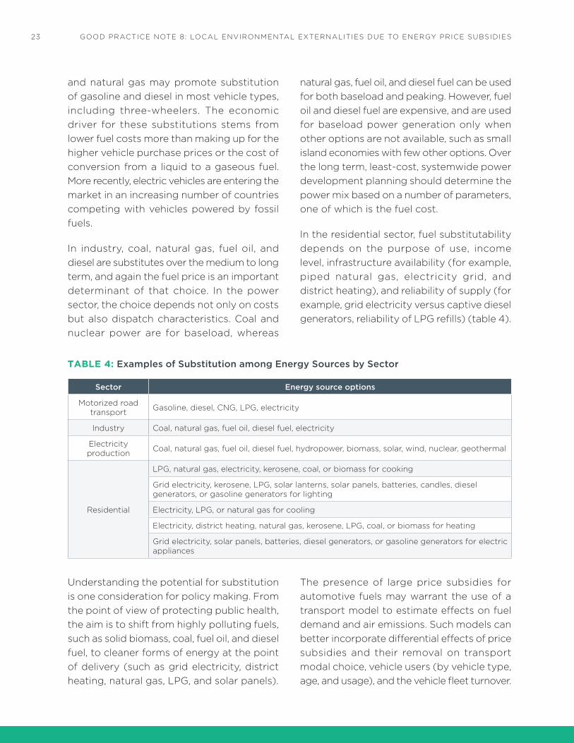
23 GOOD PRACTICE NOTE 8: LOCAL ENVIRONMENTAL EXTERNALITIES DUE TO ENERGY PRICE SUBSIDIES
and natural gas may promote substitution of gasoline and diesel in most vehicle types, including three-wheelers. The economic driver for these substitutions stems from lower fuel costs more than making up for the higher vehicle purchase prices or the cost of conversion from a liquid to a gaseous fuel. More recently, electric vehicles are entering the market in an increasing number of countries competing with vehicles powered by fossil fuels.
in industry, coal, natural gas, fuel oil, and diesel are substitutes over the medium to long term, and again the fuel price is an important determinant of that choice. in the power sector, the choice depends not only on costs but also dispatch characteristics. Coal and nuclear power are for baseload, whereas
natural gas, fuel oil, and diesel fuel can be used for both baseload and peaking. However, fuel oil and diesel fuel are expensive, and are used for baseload power generation only when other options are not available, such as small island economies with few other options. Over the long term, least-cost, systemwide power development planning should determine the power mix based on a number of parameters, one of which is the fuel cost.
in the residential sector, fuel substitutability depends on the purpose of use, income level, infrastructure availability (for example, piped natural gas, electricity grid, and district heating), and reliability of supply (for example, grid electricity versus captive diesel generators, reliability of LPG refills) (table 4).
TABLE 4: Examples of Substitution among Energy Sources by Sector
Sector Energy source options
Motorized road transport Gasoline, diesel, CNG, LPG, electricity
industry Coal, natural gas, fuel oil, diesel fuel, electricity
Electricity production Coal, natural gas, fuel oil, diesel fuel, hydropower, biomass, solar, wind, nuclear, geothermal
Residential
LPG, natural gas, electricity, kerosene, coal, or biomass for cooking
Grid electricity, kerosene, LPG, solar lanterns, solar panels, batteries, candles, diesel generators, or gasoline generators for lighting
Electricity, LPG, or natural gas for cooling
Electricity, district heating, natural gas, kerosene, LPG, coal, or biomass for heating
Grid electricity, solar panels, batteries, diesel generators, or gasoline generators for electric appliances
Understanding the potential for substitution is one consideration for policy making. From the point of view of protecting public health, the aim is to shift from highly polluting fuels, such as solid biomass, coal, fuel oil, and diesel fuel, to cleaner forms of energy at the point of delivery (such as grid electricity, district heating, natural gas, LPG, and solar panels).
The presence of large price subsidies for automotive fuels may warrant the use of a transport model to estimate effects on fuel demand and air emissions. Such models can better incorporate differential effects of price subsidies and their removal on transport modal choice, vehicle users (by vehicle type, age, and usage), and the vehicle fleet turnover.

245. HiGHER AiR EMiSSiONS FROM ENERGY PRiCE SUBSiDiES
Such models can better capture the changes in the behavior of vehicle owners with the most polluting vehicles. The 20/80 rule is often
cited as a useful first-order estimation: 20% of vehicles cause 80% of vehicle pollution.
5. HiGHER AiR EMiSSiONS FROM ENERGY PRiCE SUBSiDiES
Relative volumes of fuel consumed depend, amongst others, on relative prices, to which price subsidies contribute. Emissions of local air pollutants (per unit of energy) from fossil fuels vary greatly in relation to the type of fuel, combustion technology, and emission control technology. This is the case for primary PM2.5 as well as NOx and SO2 precursors to secondary PM2.5.
For the reasons cited in section 3 on Dispersion of Emissions, it is important to treat fuels and combustion-equipment technology as a joint system. Pollutant emissions per unit of fuel consumed vary from fuel to fuel and application to application. Mercury emissions are specific to coal, and primary PM2.5 largely to liquid and solid fuels. The same fuel can have emission factors that vary by orders of magnitude depending on the technology of the equipment used to combust it, how it is operated, and how it has been maintained. Ultra-low-sulfur diesel fuel burning in a well-maintained vehicle with state-of-the-art exhaust control devices can be as clean as a natural gas vehicle, but heavily polluting in an old overloaded truck with a dirty injector and leaking lubricant or an old backup power generator. Similarly, a new coal-fired power plant meeting the most recent directive for limiting emissions in the European Union for 2021 will be much cleaner than uncontrolled coal-fired power plants with no control devices for emissions.
MOTORIZED ROAD TRANSPORT
Where automotive fuels are subsidized, estimating PM2.5 air emissions from the road transport sector is important. Combustion of both gasoline and diesel, especially if emissions control devices are elementary or deactivated, contribute to primary particulate formation, while NOx and SO2 emissions contribute to secondary particles. The task of estimating incremental emissions is challenging. Of the three, only SO2 emissions are determined solely by fuel characteristics, increasing linearly with increasing fuel sulfur content. Particulate emissions are increased if lubricant is mixed with the fuel through leakage or in two-stroke engine vehicles. Only electric vehicles are emission free. Gaseous fuels contribute to NOx emissions, and even to small levels of particulate and SO2 emissions. Other sources of ambient PM2.5 from the sector are resuspended road dust, which is unrelated to fuel characteristics, and particulate emissions from breaking and other nonfuel vehicle sources of PM2.5. As fuel price subsidies affect both total fuel consumption and vehicle usage, all these sources of PM2.5 are affected.
Emissions from new diesel vehicles illustrate the above point. PM2.5 emissions from diesel vehicles depend on the vehicle technology, which depends in part on fuel properties, the most important of which is the level of sulfur. The evolution of limits on particulate emissions

25 GOOD PRACTICE NOTE 8: LOCAL ENVIRONMENTAL EXTERNALITIES DUE TO ENERGY PRICE SUBSIDIES
on new vehicles in the European Union over the last two decades show how emissions have declined by about 30-fold (tables 5 and 6). To enable adoption of advanced emission control devices, the level of sulfur in diesel fuel has correspondingly decreased from 2,000 ppm to 10 ppm. in-use vehicles will have higher emissions, especially those with deactivated control devices. Further,
emissions are a function of the driving cycle, and even a brand new vehicle may emit more under more aggressive driving cycles (characterized by stop-and-start driving with rapid acceleration). Many developing countries import secondhand vehicles, and vehicle maintenance practice also tends to be weaker. A number of countries still allow sulfur levels in excess of 2,000 ppm.
TABLE 5: European Union Light-Duty Diesel Vehicle Emission Standards for PM (g/km)
Corresponding sulfur level (ppm)
Light commercial vehicles (LCV) by weight class 1–3
Standard* Passenger vehicles LCV (1) LCV (2) LCV (3)
Euro 1 (1992/94) 2,000 0.14 0.14 0.19 0.25
Euro 2** (1996/98) 500 0.08 0.08 0.12 0.17
Euro 3 (2000/01) 350 0.05 0.05 0.07 0.10
Euro 4 (2005/06) 50 0.025 0.025 0.04 0.06
Euro 5 (2009/10) 10 0.005a 0.005a 0.005a 0.005a
Euro 6 (2014/15) 10 0.005a 0.005a 0.005a 0.005a
Notes: Vehicle classes LCV (1) =< 1,305 kg; LCV (2): 1,305–1,760 kg; LCV (3) > 1,760 kg.* The earlier year is for passenger vehicles and LCV (1). The later year is for LCV (2–3).** Applicable for indirect-injection engines. Slightly less stringent limits apply for direct-injection engines. a: 0.0045 g/km using the particulate measurement program procedure.Source: Adapted from www.dieselnet.com/standards/eu/ld.php.
TABLE 6: European Union Heavy-Duty Diesel Engines Emission Standards for PM (g/kWh)
Tier Year PM
Euro i1992, < 85 kW 0.612
1992, > 85 kW 0.36
Euro ii1996 0.25
1998 0.15
Euro iii 2000 0.10*
Euro iV 2005 0.02
Euro V 2008 0.02
Euro Vi 2013 0.01
Note: kW = kilowatts, kWh = kilowatt-hours.* 0.13 g for engines of less than 0.75 cubic decimeters swept volume per cylinder and a rated power speed > 3,000/minute.Source: Adapted from https://www.dieselnet.com/standards/eu/hd.php.

265. HiGHER AiR EMiSSiONS FROM ENERGY PRiCE SUBSiDiES
The simplest approach to estimating the effect of price subsidies for automotive fuels on PM2.5 emissions is to apply an average PM2.5 emission factor. This can be approximated from a profile of the diesel vehicle fleet by type of vehicle (passenger cars, light-duty vehicles, heavy-duty vehicles, buses, and trucks), vehicle use by type, the age distribution of vehicles, and any information available from emission testing and emission standards. if information about the latter is not available, then emission factors from countries with similar diesel vehicle characteristics can be applied.
it should be noted, however, that owners of different types and age of diesel vehicles will respond differently to fuel price subsidies. As a result, the effect on PM2.5 emissions from the sector may differ from that indicated by the average emission factor. Only more sophisticated modeling can capture the direction and size of this difference.
CNG is increasingly used as a motor vehicle fuel in many countries. Price subsidies to CNG are likely to be positive or relatively neutral at worst for local air pollution. in high-income countries, where gasoline vehicles are very clean, the environmental benefits may be very small unless CNG is replacing high emitters, which is unlikely since high emitters tend to be old vehicles and there is no economic case for conversion from gasoline to CNG. in developing countries where high emitters are much more prevalent, substituting gasoline for CNG could bring measurable benefits. Substituting CNG for diesel is likely to bring measurable benefits in almost all cases.
RESIDENTIAL SECTOR
Household air pollution, which is prevalent especially among low- and lower-middle-income households, is estimated to cause
nearly 3 million deaths per year (GBD 2015 risk factors collaborators 2016). in low- and lower-middle-income countries, price subsidies for LPG, natural gas, or biogas large enough to shift a significant number of households away from traditional use of solid fuels for cooking and heating will have the largest effects on air pollution and health10 of all energy price subsidies in the residential sector. However, the magnitude of price subsidies needed to effect fuel switching on a scale that would deliver measurable health benefits is beyond the means of virtually all governments.
To the extent that price subsidies lead to lower use of solid fuels, the benefits depend on the degree of fuel switching, because households are known to “stack” fuels—using multiple fuels even as they shift away from solid fuels—rather than climb up a fuel ladder, as previously thought (Masera, Saatkamp, and Kammen 2000). if they continue to use solid fuels, the benefits of adding gaseous fuels may be greatly diminished. Fuel stacking in turn can make the relationship between fuel consumption and PM2.5 concentrations highly nonlinear.
Similarly, subsidies for district heating to make it affordable may shift households away from burning coal or solid biomass for heating, again reducing household air pollution. if the heat generation plant providing heat is fueled by coal and is located near population centers, however, outdoor air pollution may offset some of the benefits of reduction in indoor air pollution. Price subsidies for electricity that shift households away from solid fuel use for cooking and heating, or from captive diesel generators, would also reduce air pollution and improve health outcomes. A methodology for estimating health effects of such subsidies is presented in section 8.

27 GOOD PRACTICE NOTE 8: LOCAL ENVIRONMENTAL EXTERNALITIES DUE TO ENERGY PRICE SUBSIDIES
INDUSTRY
Primary PM2.5 emissions from petroleum product consumption in the industry can be calculated from standard emission factors that do not exhibit the large variations observed among motorized vehicles. Primary PM2.5 emissions from natural gas are minimal and can be ignored for analytical purposes. Primary PM2.5 from coal combustion will depend on the industrial sector in which coal is used and any abatement technology used in it. Any available in-country studies should be used to inform the analysis. in their absence, emission factors from similar sectors in other countries can be applied.
The contribution of secondary PM2.5 from oil products, natural gas, and coal may be substantial if industrial fuel consumption is large. This may be estimated as a sector share of ambient secondary PM2.5, with ambient secondary PM2.5 estimated from apportionment studies discussed in the next section.
ELECTRICITY
As Good Practice Note 1 explains, the fact that electricity tariffs do not recover costs does not automatically imply the presence of price subsidies. To the extent that price subsidies exist (which is the case if there is underpricing, as defined in Good Practice Note 1), lower prices would lead to higher electricity consumption in the absence of constraints on supply. However, almost all developing countries face rising demand for electricity. in low- and lower-middle-income countries in particular, where per capita electricity consumption is much lower than that in high-income countries and the growth rates of electricity consumption are correspondingly higher, the power infrastructure has frequently suffered from years and even decades of underinvestment,
and as a result power shortages are common. in such circumstances, price subsidies may merely determine the distribution and size of the unmet demand. increased production to meet incremental consumption may come from any electricity sources, fossil fuels or otherwise, depending on what will provide the marginal supply. if new capacity has to be added, so-called build-margin grid-emission factors (emission factors of new generation capacity) may and are likely to be different from operating-margin factors (emission factors of existing generation capacity). if the power sector in the country in question does not have build-margin emission factors, options being proposed by a group of multilateral development banks may be considered.11
Existing studies can be used to estimate operating-margin PM2.5 emission factors. if such studies do not exist, emissions can be approximated from known fuel and plant characteristics, such as the type of fuel (for example, coal or natural gas) and its characteristics (for example, ash and sulfur content of coal); the type of plant (open cycle or combined cycle gas turbine, steam boiler, reciprocating motor, fluidized bed); operating characteristics (baseload, peaking, load factor); and operation and performance of any particulate, SO2, and NOx emission abatement technology installed. For build-margin emission factors, manufacturers’ specifications and estimated performance deterioration may be used.
To help the poor consume electricity, subsidized connection fees and volume-differentiated tariffs may be offered. They are effective, provided the lifeline block is kept relatively small to match subsistence-level consumption. As Good Practice Note 1 explains, increasing block tariffs by contrast may benefit the nonpoor disproportionately

286. POPULATiON EXPOSURE ASSESSMENT
because every consumer, however rich, benefits from the lifeline rate. This is especially so if the electrification rate is relatively low, those with access to grid electricity are primarily the better-off in urban areas, and the first block (sold at the lifeline rate) is relatively large. The same concepts apply to the other two forms of network energy, natural gas and district heating. in all cases, targeting requires accurate metering of every household. This requirement is not met in many countries, where multiple houses are connected to a single meter, households are billed according to estimated consumption, meters are not accurate, or any combination of these shortcomings.
Because the poor consume little electricity, their impact on the country’s overall electricity consumption will likely be very small. in most low- and lower-middle-income countries, where household use of solid fuels is prevalent, electricity is not used for cooking, especially among the poor, and hence the health benefits of providing electricity will also likely be small:
electricity would displace kerosene for lighting, but the poor may continue to cook and heat with solid fuels.
Switching from diesel generators to grid electricity would decrease local air pollution. The decision to use diesel generators is driven by the consumer’s assessment of power supply reliability. if price subsidies are contributing significantly to power outages, removing such subsidies would contribute to increasing reliability, but that would take time. Because poor reliability is caused by a number of factors and not just by price subsidies, it may be difficult to disentangle the contribution of price subsidies to power outages.
Subsidies for solar, wind, and geothermal power should reduce emissions, although if the subsidies make coal more attractive than natural as, as has happened in recent years in some European countries, the policy may backfire and increase coal consumption at the expense of natural gas, with a net increase in pollutant emissions.
6. POPULATiON EXPOSURE ASSESSMENT
Estimating population exposure to air pollution due to incremental emissions from energy price subsidies is arguably the most elaborate, data-intensive, and time-consuming task. Two broad approaches may be used for this purpose: (a) dispersion modeling, and (b) intake fractions.
DISPERSION MODELING
An example of the use of dispersion modeling to estimate the health effects of air pollution is the program, “Global Burden of Disease from Major Air Pollution Sources (GBD MAPS).” GBD
MAPS applies the GBD project methodology to estimate health effects.12 The program is estimating the disease burden due to outdoor air pollution from coal burning and other major sources in China (nationally and by province), india, and Eastern Europe using the GBD framework.
The study in China used the chemical transport model GEOS-Chem and calculated the contributions of coal combustion, industry (noncoal), transportation, domestic biomass burning, and open burning to population-weighted ambient PM2.5 concentrations at the

29 GOOD PRACTICE NOTE 8: LOCAL ENVIRONMENTAL EXTERNALITIES DUE TO ENERGY PRICE SUBSIDIES
national and provincial level. Coal combustion was evaluated from power plants, industry, and domestic coal use.13 The study also estimated the health effects of PM2.5 air pollution from various sources, using the health-risk functions from the GBD project (GBD MAPS WG 2016). This approach and model can in principle be applied to assess the health effects of energy price subsidies once changes in energy consumption and emissions from price subsidies are estimated.
By incorporating population distribution into dispersion models, it is possible to estimate the intake fractions (the fractions of emissions inhaled by the population exposed to the emissions), which can be used to estimate the health effects of emissions. Zhou and others (2006) used such modeling to estimate the emission intake fractions from power plant sites throughout China, as discussed below.
INTAKE FRACTIONS
A measure of human exposure is the emission intake fraction, which estimates the fraction of a metric ton of emissions breathed in by
the population. The larger the intake fraction, the larger the health effects per metric ton of emissions.
Apte and others (2012) estimated the intra-urban intake fraction of distributed ground-level emissions of primary pollutants in more than 3,600 cities worldwide with a population greater than 100,000. intake fractions were based on location-specific geographic, meteorological, and demographic data. Population-weighted intra-urban intake fractions by country ranged from less than 10 to more than 100 ppm, and by major city from less than 5 to more than 250 ppm (or gram per metric ton of emissions). The population-weighted intake fractions by country are reported in the supplementary information note of Apte and others (2012).
Population-weighted mean intake fractions by region and city size are presented in table 7, which shows that mean intake fractions vary more by city population than by region. The highest mean intake fractions are in South and Central Asia, Southeast Asia, East Asia and Pacific, and Sub-Saharan Africa.
TABLE 7: Population Weighted Mean Intra-Urban Intake Fractions of Distributed Ground-Level Emissions (ppm)
Small cities(100,000–600,000)
Medium cities(600,000–3 million)
Large cities(> 3 million)
All cities(> 100,000)
South and Central Asia 15 36 106 55
Southeast Asia 20 46 67 48
East Asia and Pacific 22 49 70 44
Sub-Saharan Africa 18 38 98 43
Latin America 13 32 69 41
North Africa 10 27 57 32
Europe and Japan 10 22 55 30
Western Asia 12 27 41 26
Land-rich developed 7 15 30 20
World 15 35 65 39
Source: Apte and others 2012, supplementary information.

306. POPULATiON EXPOSURE ASSESSMENT
Humbert and others (2011) summarized the work of an international expert group on the integration of human exposure to PM into life cycle impact assessment (LCiA) within the UNEP/SETAC Life Cycle initiative. The authors reported recommended intake fractions for primary PM2.5 and secondary PM2.5 from SO2, NOx, and ammonia (NH3) precursors. Recommended global values for urban and rural areas are reported in table 8. The distributed ground-level intake fraction
for primary PM2.5 in urban areas is similar to the global population-weighted mean intake fraction in Apte and others (2012). The intake fractions in rural areas are about one tenth of the urban fractions and decline by stack height. The intake fractions for secondary PM2.5 are expressed in grams of PM2.5 per metric ton of precursor emissions, with similar recommended values for urban and rural areas.
TABLE 8: Summary of Recommended Intake Fractions (ppm)
Height Primary PM2.5
Urban Rural
Ground-level emissions 44 3.8
Low stack (25 meters) 15 2.0
High stack (100 meters) 11 1.6
Emission source weighted average* 26 2.6
Precursors Secondary PM2.5
Urban Rural
Sulfur dioxide (SO2) 0.99 0.79
Nitrogen oxides (NOX) 0.2 0.17
Ammonia (NH3) 1.7 1.7
* Weighted by typical emission release height (ground, low, and high).Source: Humbert and others 2011.
By region, the highest weighted urban intake fractions of primary PM2.5 are in Latin America
and Southeast Asia. The highest rural intake fraction is in Southeast Asia (table 9).
TABLE 9: Recommended PM2.5 Intake Fractions by Region
Urban Rural
Generic 26 2.6
United States 15 0.92
Latin America 29 0.75
Europe 18 2.1
Africa and the Middle East 25 1.1
Central Asia 20 1.3
Southeast Asia 29 4.6
Note: Data in this table are weighted by typical emission release height (ground, low, and high).Source: Humbert and others 2011.

31 GOOD PRACTICE NOTE 8: LOCAL ENVIRONMENTAL EXTERNALITIES DUE TO ENERGY PRICE SUBSIDIES
in a seminal study in China, Zhou and others (2006) selected 29 power plant sites throughout the country and estimated intake fractions at each site. A detailed long-range atmospheric dispersion model, CALPUFF, was used to model the increase in concentrations due to emissions from selected power plants. Mean intake fraction of primary PM3
14 was 6 ppm, ranging from 1.7 to 12 ppm across
sites (table 10). The mean intake fraction is comparable to the estimation for rural areas in Southeast Asia in table 9, albeit somewhat higher. intake fractions for secondary PM3 were also estimated as grams of sulfate or nitrate per metric ton of SO2 or NOx emissions. The mean intake fractions are substantially higher than the global mean recommended by Hubert and others (2011).
TABLE 10: Intake Fraction Estimates across 29 Power Plant Sites throughout China (ppm)
Mean Minimum Maximum
Primary PM3 6.1 1.7 12.0
Sulfate 4.4 0.7 7.3
Nitrate 3.5 0.8 7.1
Source: Zhou and others 2006.
Regression models were developed to interpret the intake fraction values and allow for extrapolation to other sites. Explanatory variables were meteorological proxies, such as climate region and precipitation, and population at various distances from the sources. Differences in population distribution explain a high portion of the differences in the intake fractions across sites. The meteorological regime also had a significant influence on intake fractions (Zhou and others 2006).
INTAKE FRACTION APPLICATIONS
Cropper and others (2012) estimated the health effects of emissions from coal-fired power plants in india by applying the intake-fraction regression models in Zhou and others (2006) used in China and adjusting for differences in population distributions and rainfalls. All coal-fired power plants in india have particulate abatement equipment, but practically none had sulfur abatement technology at the time of the study. The study
estimated that health effects due to sulfate- and nitrate-based secondary PM2.5 were, on average, 17 and 4 times larger, respectively, than health effects due to primary PM2.5, even though indian coal has a low average sulfur content of 0.5%. The findings may point to the importance of incorporating intake fractions for secondary PM2.5 when assessing the health effects of electricity price subsidies or price subsidies for fuels used in electricity generation.15
Parry and others (2014) applied intake fractions to estimate country-level health effects of primary and secondary PM2.5 emissions from fossil fuels in order to estimate corrective taxes. The paper by Apte and others (2012) was used for intra-urban intake fractions of distributed ground-level primary PM2.5 emissions from road transportation and residential sources. This was combined with the findings of Humbert and others (2011) to estimate country-specific intake fractions for SO2 and NOx. The intake-fraction regressions in Zhou and others (2006) were used to

326. POPULATiON EXPOSURE ASSESSMENT
estimate country-specific intake fractions from power plants.
PROPOSED APPROACH
This section outlines the proposed approaches to estimating population exposure to air pollution due to incremental emissions from energy price subsidies from different sources.
Distributed Ground-Level Emissions
The proposed approach for distributed ground-level emissions is to consider three areas: urban areas with a population greater than 100,000, urban areas with a population under 100,000, and rural areas. The country-specific population-weighted intra-urban intake fractions from Apte and others (2012) is the recommended choice for urban areas with a population greater than 100,000. The value of 3.8 ppm from Humbert and others (2011) is proposed for vehicular emissions in rural areas, including inter-urban vehicle transportation. This value may be made country-specific by adjusting for differences in rural population density. A value between the intake fraction for small cities (100,000–600,000) in Apte and others (2012) and the rural value can be applied to urban areas with a population less than 100,000.
For secondary PM2.5, the intake fractions for SO2 and NOx from Humbert and others (2011) can be scaled by the country-specific intake fractions for primary PM2.5 in Apte and others (2012), an approach adopted by Parry and others (2014).
Power Plant Emissions
The proposed approach for power plant emissions follows the procedures used by Cropper and others (2012) and by Parry and
others (2014), and estimates country-specific intake fractions from the intake fraction regressions in Zhou and others (2006). These intake fractions can be applied to both coal- and natural gas–fired power plants.
Industry
intake fractions of emissions from fuels consumed by the industrial sector will likely fall somewhere between the intake fractions from power plants and distributed ground-level emissions and will be influenced largely by industrial locations that can be assessed in country assessments of subsidies. Most cottage industries belong to distributed ground-level missions.
Baseline Outdoor PM2.5 Concentrations
Because the relationships between PM2.5 and health outcomes are nonlinear (see next section), data on initial or prevailing outdoor PM2.5 concentrations are essential to estimate the health effects of higher fuel consumption caused by energy price subsidies. Ambient concentrations must be established at the selected geographic or demographic scale to analyze the impacts of energy price subsidies. The proposed scale is similar to that discussed in the section on population exposure assessment for distributed ground-level emissions: urban areas with a population greater than 100,000, urban areas with a population under 100,000, and rural areas.
Population-weighted average ambient PM2.5 concentrations in areas affected by emissions from power plants may be best approximated using the nationwide population-weighted average ambient PM2.5, as emissions from this source are dispersed over large geographic areas. For emissions from road transport and other urban ground-level distributed sources,

33 GOOD PRACTICE NOTE 8: LOCAL ENVIRONMENTAL EXTERNALITIES DUE TO ENERGY PRICE SUBSIDIES
the best approximation will generally be urban-population-weighted average ambient PM2.5 for the share of fuels consumed in urban areas, and the rural-population-weighted average ambient PM2.5 for the share of fuels consumed outside of urban areas. For fuels used by industry, an average of nationwide and urban concentrations may well represent population exposures in areas with industrial emission sources.
Ambient ground- leve l mon i tor ing measurements will rarely be available to establish PM2.5 concentrations accurately at this scale. Assumptions for approximations will, therefore, have to be made. One option is to apply ambient concentrations estimated from satellite/transport models, an approach used in the GBD project (Brauer and others 2016; van Donkelaar and others 2015, 2016). For urban areas, the priority will be to assemble as much of available ground-level monitoring measurement data as possible.
The global estimates used by the GBD project are presented below.
Global estimates of annual PM2.5 concentrations at 0.1° × 0.1° spatial resolution for the GBD Study 2013 by the institute for Health Metrics and Evaluation have recently been published (Brauer and others 2016). The estimates were produced by combining satellite-based estimates, chemical transport model simulations, and ground measurements from 79 different countries. The estimates indicate that annual PM2.5 concentrations in large parts of North Africa, Middle East, and Asia exceeded the World Health Organization’s (WHO) interim Target 3 of 35 micrograms per cubic meter (µg/m3) (figure 2). However, it is worth highlighting that the accuracy of these global estimates is influenced by the availability and calibration of ground-level monitoring measurements of PM2.5, which are relatively scarce in many developing countries (van Donkelaar and others 2015).
FIGURE 2: Estimated Annual Average PM2.5 (µg/m3)
Source: Brauer and others 2016.
<10 (meets WHO Guideline)≥ 10 (WHO Guideline)≥ 15 (WHO Interim Target 1)≥ 25 (WHO Interim Target 2)≥ 35 (WHO Interim Target 3)
2013 Annual Average PM2.5 (µg/m3)

347. HEALTH EFFECTS
7. HEALTH EFFECTS
This section presents the health effects due exposure to air pollution.
OUTDOOR AIR POLLUTION
This section presents the health effects caused by outdoor air pollution.
Mortality
The health effects of incremental energy consumption due to energy price subsidies are estimated by the term in equation 1 in section 2, which represents a change in health effects (δD) from a change in emissions (δE). This term can be expressed as
(3)
where m is baseline annual cases of the health outcomes (for example, the total number of premature deaths) and PIF is the potential impact fraction of health outcomes associated with δE, expressed as the percentage change in health outcomes associated with a change in PM2.5 emissions (see below). By using intake fraction equations (see annex 1), equation 3 becomes
(4)
where iF is the intake fraction of emissions (ppm); P is exposed population; K= Qd * 365 * 10
-6 where Qd is the breathing rate of air (m3/day/person); and x is PM2.5 concentrations. Equation 4 says that health effects per metric ton of changes in PM2.5 emissions are a function of the product of the intake fraction and the potential impact
fraction (PIF) of health outcomes per change in PM2.5 concentrations.
The PIF is estimated using the relative-risk functions from the GBD project. These functions are nonlinear (Pope and others 2009, 2011; Burnett and others 2014; GBD 2015 risk factors collaborators 2016). Thus the magnitude of the PIF per change in concentrations of PM2.5 is a function of initial concentration.
The potential impact fraction from a change in PM2.5 concentrations is
where Pi and P'i are the percentage of population exposure before and after a change in PM2.5 concentrations and RR is the relative risk of health outcomes at PM2.5 concentrations at the midpoint of concentrations xi and xi-1 (see annex 2).
The RR from the integrated-exposure-response (iER) function used by the GBD Study 2015 are published in GBD 2015 risk factors collaborators (2016)17 (figure 3). The RRs of ischemic heart disease (iHD) and cerebrovascular disease (stroke) are the smallest for PM2.5 concentrations larger than 30–40 µg/m3 and the RR of acute lower respiratory infection (ALRi) is the largest at PM2.5 concentrations greater than 40 µg/m3.18 Globally, iHD accounts for 36% of deaths from outdoor PM2.5, stroke for 21%, chronic obstructive pulmonary disease (COPD) for 20%, ALRi for 16%, and lung cancer for 7%, according to GBD 2015.
δD
δE
δD = mPIF
,δE δE
δD =m
IFPIF
,δE KP δx
PIF = [ PiRRXi + Xi-1
2-
ni=1 P’iRR
Xi + Xi-1
2]/[ ], (5)n
i=1 PiRRXi + Xi-1
2n
i=1

35 GOOD PRACTICE NOTE 8: LOCAL ENVIRONMENTAL EXTERNALITIES DUE TO ENERGY PRICE SUBSIDIES
The RRs are derived from studies of long-term exposure to outdoor air PM2.5, secondhand tobacco smoking, exposure to smoke from household solid cooking fuels, and active tobacco smoking (Burnett and others 2014). This provides a risk function that can be applied to a wide range of outdoor PM2.5 concentrations around the world as well as to high household air pollution levels of PM2.5 from the combustion of solid fuels.
The risk functions are nonlinear, with declining marginal health effects at higher PM2.5 concentrations. Thus, the health effects of air pollution caused by energy price subsidies greatly depend on initial concentrations of PM2.5.
Morbidity
The empirical research literature presents a whole set of morbidity health outcomes from ambient PM2.5 and other air pollutants. The literature most often expresses the risk of these health outcomes as percentage changes relative to the baseline incidence or prevalence. However, reliable baselines are not
readily available in most developing countries without conducting extensive surveys.
Monetary valuation of many of these morbidity health outcomes is also a complex task. The studies that have valued both mortality and morbidity from ambient PM2.5 generally find that mortality counts for about 80% of total health costs. Thus the substantial efforts required to accurately estimate and value morbidity from exposure to incremental PM2.5 concentrations caused by energy price subsidies are not likely to be worth the resources required for the purpose of improving the overall estimation of the monetary value of health effects of price subsidies.
An alternative, simpler approach is to estimate morbidity by applying the disease burden from morbidity per premature death from ambient PM2.5 reported by the GBD project. The disease burden from morbidity is reported as “years of life lost to disability” (YLD) and is generally in the range 0.5–1.0 YLD per death according to the GBD project. These years of life lost can be converted to days of illness by multiplying YLD by 365 days per year and
FIGURE 3: Relative Risks of Major Health Outcomes Associated with PM2.5 Exposure
1.0
1.1
1.2
1.3
1.4
1.5
1.6
1.7
1.8
10 15 20 25 30 35 40 45 50 55 60 65 70 75 80 85 90 95 100
Stroke IHD COPD LC ALRI
Annual average PM2.5 (µg/m3)
Source: GBD 2015 risk factors collaborators 2016.
367. HEALTH EFFECTS
dividing by the average disability weight for the health outcomes associated with ambient PM2.5 (typically 0.1–0.2). The estimated days of illness can then be monetized (see the next section).
HOUSEHOLD AIR POLLUTION
This section presents the health effects caused by household air pollution.
Mortality
Kerosene, LPG, electricity, and natural gas are alternatives to solid fuels for cooking, which are prevalent in low- and lower-middle-income countries. Household air pollution is estimated to cause nearly 3 million deaths per year (GBD 2015 risk factors collaborators 2016). Price subsidies for cleaner alternatives may reduce household air pollution markedly if households using solid fuels switch substantially or entirely to these alternatives. Even in such circumstances, however, if neighbors continue to burn solid fuels, high outdoor PM2.5 concentrations caused by the neighbors’ activities affect indoor concentrations in the dwellings of those using only clean forms of energy, diminishing health benefits. in practice, switching is rarely complete or even substantial among the poor, who continue to use cheap or free solid biomass or coal for cooking and heating, supplemented by cleaner forms of energy for limited activities. Kerosene that is pressurized before combustion burns cleanly, but otherwise kerosene combustion (as in wick stoves) can be quite polluting, although not nearly as much as combustion of solid fuels. Because health effects as a function of ambient concentrations of PM2.5 are nonlinear and decline slowly with falling ambient concentrations at relatively high levels, partial switching to cleaner forms of
energy may have limited or even undetectable health effects.
There is little information on the extent of switching to cleaner forms of energy across households. Many households use multiple forms of energy for cooking and heating. And yet most household surveys20 report only the primary source of energy for cooking, while many do not ask about heating. information on quantities consumed is seldom available, and even when data are collected, they are plagued by inaccuracy.
The most optimistic (and also the most unrealistic) approach is to assume that the price subsidies lead households to switch entirely to cleaner forms of energy and stop using solid fuels altogether. This provides an upper bound on the benefits of price subsidies A more reasonable—although still not realistic—approach is to assume that all households will start using cleaner forms of energy and will also continue to use one or more solid fuels, reducing solid fuel consumption by the amount that corresponds to an overall increase in the consumption of the subsidized energy obtained using relevant price elasticities. This scenario does not envisage an increase in overall household energy use, as found by Masera, Saatkamp, and Kammen (2000).
in the first case, the first step in estimating the household air pollution effects of subsidies is to estimate the percentage change in households using solid fuels (S):
(6)
where S is the number of households using solid fuels; L is the number of households using cleaner forms of subsidized energy; T is the total number of households; subscripts “0” and
S =S1 -S0 =
L0 - L1 = - L1 L S0 S0 T(1+L) - L1

37 GOOD PRACTICE NOTE 8: LOCAL ENVIRONMENTAL EXTERNALITIES DUE TO ENERGY PRICE SUBSIDIES
“1” denote households in the absence and in the presence of price subsidies, respectively; and L is the percentage change in the number of households using cleaner forms of subsidized energy. if households switch to exclusive use of clean energy, then L is approximately equal to the percentage change in the consumption of cleaner energy, estimated by the methods discussed in the previous section.
The change in health effects (such as the number of premature deaths per year) is then
(7)
where D1 is the number of nationwide cases of health outcomes per year associated with household air pollution from solid fuels in the presence of price subsidies. D1 can be estimated from current patterns of household energy use and health risk methodology from the GBD project.
in the second case, it is assumed that all households respond to the price subsidies and will use a little less solid fuels and a little more of cleaner energy. Percentage change in aggregate solid fuel consumption, ES is approximated by
(8)
where ES is aggregate solid fuel consumption at prevailing price subsidies for clean forms of energy; ΔES and ∆ECE are the respective changes in the consumption of solid fuels and clean energy due to price subsidies, with the assumption that ΔES = -∆ECE; and ES
is expressed in the same energy unit as that for clean energy.21
The next step is to estimate the change in household air pollution concentrations from the change in solid fuel use. The percentage change in concentrations among households using solid fuels may simply be approximated as being equal to ES in equation 8.
The change in health effects as a result of changes in household air pollution concentrations among households using solid fuels can be estimated using the PIF and health-risk functions from the GBD project. As the health-risk functions are nonlinear with declining marginal health effects, the estimated health effects in the first case will be larger than in the second case.
Morbidity
As with morbidity due to outdoor PM2.5 pollution, morbidity from household air pollution can be estimated by applying the disease burden from morbidity per premature death from household PM2.5 air pollution reported by the GBD project. The disease burden from morbidity is reported as YLD and is generally in the range of 1.0–2.5 YLD per death according to the GBD project.22 These years of life lost can be converted to days of illness by multiplying YLD by 365 days per year and dividing by the average disability weight for the health outcomes associated with ambient PM2.5 (for example, 0.1–0.2). The estimated days of illness can then be monetized (see next section).
∆D =SD1
1+S
ES = ∆ES = - ∆ECE
ES ES

388. THE VALUE OF HEALTH EFFECTS
8. THE VALUE OF HEALTH EFFECTS
This section presents methods to estimate the value of mortality and morbidity caused by air pollution.
MORTALITY
The predominant measure of the welfare cost of a premature death used by economists is the value of statistical life (VSL) (annex 3). Reliable VSL studies are available only from a minority of countries globally. A common approach to estimating VSL in a country that lacks such studies is therefore to use a benefit transfer based on meta-analyses of VSL studies from other countries. Narain and Sall (2016) presents such a benefit-transfer methodology for valuing mortality from air pollution, drawing on the empirical literature of VSL, especially studies on the members of the Organisation for Economic Co-operation and Development (OECD) (OECD 2012). The proposed benefit transfer function is
(9)
where VSLc,n is the estimated VSL for country c in year n; VSLOECD is the average base VSL in the sample of OECD countries with VSL studies (US$3.83 million); Yc,n is GDP per capita in country c in year n; YOECD is the average GDP per capita for the sample of OECD countries (US$37,000); and ∈ an income elasticity of 1.2 for low- and middle-income countries and 0.8 for high-income countries. All values are in purchasing power parity (PPP) prices. VSLc,n must, therefore, be converted to local currency using PPP exchange rates, available in the World Development indicators by the World Bank.
MORBIDITY
The cost of morbidity includes work absenteeism and medical treatment. The willingness to pay to avoid pain and suffering can also be added to this cost, but estimates are generally not available for most countries. if a day of illness is valued at 50–100% of average daily wage rates to account for partial work absenteeism and medical expenses, then the cost of one YLD is about 5–10 times GDP per capita.23
The cost of morbidity per death from ambient PM2.5 is then 2.5–10 times GDP per capita for 0.5–1.0 YLD per death. By contrast, the cost of mortality per death or VSL is about 70 times GDP per capita in lower-middle-income countries, per equation 9. The cost of morbidity is therefore only about 4–14% of the cost of mortality.
Studies that have valued both mortality and morbidity from ambient PM2.5 pollution generally find that morbidity accounts for approximately 20% of total health costs. A reasonable approach to valuing morbidity from ambient PM2.5 pollution may, therefore, be to use a morbidity-cost share of 10–20%, with the lower bound being about the midpoint of the estimate presented above.
The cost of morbidity per death from household PM2.5 air pollution is higher than from ambient PM2.5 pollution, because YLD from this pollution is 1.0–2.5 per death. The cost of morbidity per death is therefore 5–25 times GDP per capita. This is 7–35% of the cost of mortality, with a midpoint of about 20% if the cost per death or VSL is about 70 times GDP per capita.
VSLc,n = VSLOECD *(Yc,n )∈
YOECD

39 GOOD PRACTICE NOTE 8: LOCAL ENVIRONMENTAL EXTERNALITIES DUE TO ENERGY PRICE SUBSIDIES
A reasonable approach to valuing morbidity from household PM2.5 air pollution may, therefore, be to use a morbidity cost share of 20–30%, with the lower bound being in the neighborhood of the midpoint of the estimate presented above, and the upper bound reflecting a premium for pain and suffering associated with illness. These costs of morbidity can be made specific to a country by using country-level data on YLD per death, wage rates, and VSL.
USING THE VALUE OF HEALTH EFFECTS TO INFORM POLICY OPTIONS
Estimating and valuing the health effects of air pollution can inform potential interventions to reduce price subsidies with negative environmental and health effects or, alternatively, to evaluate price subsidies with positive effects.
Household air pollution is taken here as an illustration. Billions of people around the world do not have access to energy that is clean at the point of delivery. They use solid fuels for cooking and heating, such as coal, wood, agricultural residues, animal dung, and trash. Burning of solid fuels in traditional stoves, and often with inadequate ventilation, results in high concentrations of air pollutants within households. Studies in countries such
as Bolivia, Guatemala, Honduras, Mexico, Nicaragua, and Peru have found indoor air pollution concentrations that far exceed anything that might be considered reasonably safe for public health.
Exposure to indoor air pollution, particularly PM2.5, causes several illnesses. They include cardiovascular disease, COPD, and lung cancer among adults, and ALRi among young children (Lim and others 2012). Women and children face greater risks from indoor air pollution because they typically spend more time at home and often near the sources of combustion.
Setting aside pain and suffering, there are economic costs associated with adverse health effects caused by household air pollution. They include medical expenses, forgone wages, and loss of productivity. Added together, these losses can represent a significant economic burden. Table 11 shows calculated premature deaths and days of illness attributed to household air pollution and their associated costs in several Latin American countries and subnational jurisdictions, using the methodologies described in this note. At the national level, the costs imposed by household air pollution are equivalent to up to 1.76% of GDP in Bolivia, and subnationally, they represent up to 2.88% of GDP in Apurimac, Peru.
TABLE 11: Premature Deaths and Days of Illness Caused Annually by Household Air Pollution and Their Associated Costs in Selected Jurisdictions
Country Deaths Days of Illness (million) Cost (% of GDP)
Bolivia (2014) 3,082 1.76%
Mexico (2013) 12,931 77 0.58%
Peru (2012) 6,114 65.5 1.31%
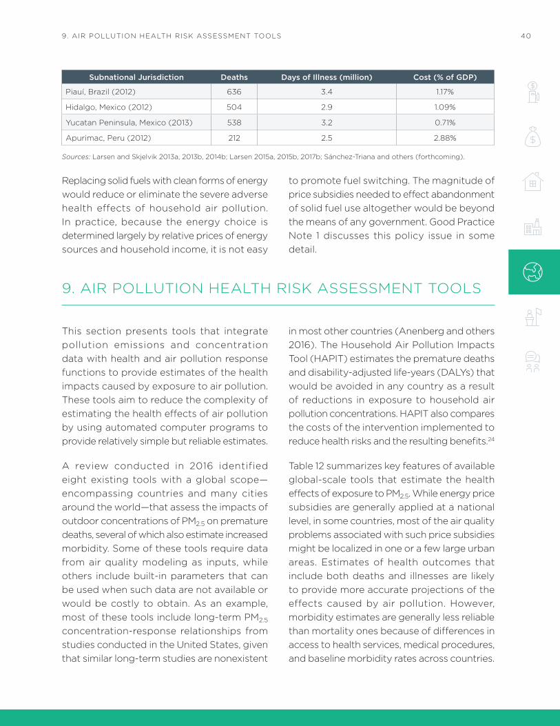
409. AiR POLLUTiON HEALTH RiSK ASSESSMENT TOOLS
Subnational Jurisdiction Deaths Days of Illness (million) Cost (% of GDP)
Piauí, Brazil (2012) 636 3.4 1.17%
Hidalgo, Mexico (2012) 504 2.9 1.09%
Yucatan Peninsula, Mexico (2013) 538 3.2 0.71%
Apurimac, Peru (2012) 212 2.5 2.88%
Sources: Larsen and Skjelvik 2013a, 2013b, 2014b; Larsen 2015a, 2015b, 2017b; Sánchez-Triana and others (forthcoming).
Replacing solid fuels with clean forms of energy would reduce or eliminate the severe adverse health effects of household air pollution. in practice, because the energy choice is determined largely by relative prices of energy sources and household income, it is not easy
to promote fuel switching. The magnitude of price subsidies needed to effect abandonment of solid fuel use altogether would be beyond the means of any government. Good Practice Note 1 discusses this policy issue in some detail.
9. AiR POLLUTiON HEALTH RiSK ASSESSMENT TOOLS
This section presents tools that integrate pollution emissions and concentration data with health and air pollution response functions to provide estimates of the health impacts caused by exposure to air pollution. These tools aim to reduce the complexity of estimating the health effects of air pollution by using automated computer programs to provide relatively simple but reliable estimates.
A review conducted in 2016 identified eight existing tools with a global scope—encompassing countries and many cities around the world—that assess the impacts of outdoor concentrations of PM2.5 on premature deaths, several of which also estimate increased morbidity. Some of these tools require data from air quality modeling as inputs, while others include built-in parameters that can be used when such data are not available or would be costly to obtain. As an example, most of these tools include long-term PM2.5 concentration-response relationships from studies conducted in the United States, given that similar long-term studies are nonexistent
in most other countries (Anenberg and others 2016). The Household Air Pollution impacts Tool (HAPiT) estimates the premature deaths and disability-adjusted life-years (DALYs) that would be avoided in any country as a result of reductions in exposure to household air pollution concentrations. HAPiT also compares the costs of the intervention implemented to reduce health risks and the resulting benefits.24
Table 12 summarizes key features of available global-scale tools that estimate the health effects of exposure to PM2.5. While energy price subsidies are generally applied at a national level, in some countries, most of the air quality problems associated with such price subsidies might be localized in one or a few large urban areas. Estimates of health outcomes that include both deaths and illnesses are likely to provide more accurate projections of the effects caused by air pollution. However, morbidity estimates are generally less reliable than mortality ones because of differences in access to health services, medical procedures, and baseline morbidity rates across countries.

41 GOOD PRACTICE NOTE 8: LOCAL ENVIRONMENTAL EXTERNALITIES DUE TO ENERGY PRICE SUBSIDIES
in terms of format, web-based systems are the most accessible because they can be run using a freely available internet browser. Several tools use spreadsheets, with which many potential users are already familiar. A few tools require downloading custom software. Two tools are proprietary and the remaining five use open-source codes. Aside from cost savings, the main advantage of
open-source codes is that the algorithms and data sets used for estimation are transparent. A key consideration in tool selection is the availability of the inputs needed to run it. Most models require air quality modeling data to be entered by the user, but some reduced-form tools can be used to obtain broad estimates by using built-in parameters (Anenberg and others 2016).
TABLE 12: Key Characteristics of Air Pollution Health Risk Assessment tools
Tool Spatial resolution Health outcome Format Required user input (information source)
AirCountsa City level Mortality cases Web-based, proprietary
Emissions (primary PM2.5 intake fraction)
AiRQ 2.2b Regional, national, or city-level
Mortality and morbidity cases, DALYs and YLLs
Software download, open source
Concentration (any concentration input by user)
BenMAP-CEc Regional, national, or city-level
Mortality and morbidity cases, DALYs and YLLs
Software download, open source
Concentration (any concentration input by user)
Environmental Burden of Diseased
Regional, national, or city-level
Mortality and morbidity cases, DALYs and YLLs
Microsoft Office, open source
Concentration (any concentration input by user)
iOMLiFETe Regional, national, or city-level
Mortality and morbidity cases, DALYs and YLLs
Microsoft Office, open source
Concentration (any concentration input by user)
LEAP-iBCf National Mortality cases Microsoft Office, open source
Emissions (reduced-form chemical transport model)
SiM-Airg Regional and city level
Mortality and morbidity cases
Microsoft Office, open source
Emissions (regional or urban atmospheric chemistry model)
TM5-FASSTh Regional and national
Mortality cases, DALYs and YLLs
Microsoft Office, proprietary
Emissions (reduced-form chemical transport model)
a. http://www.aircounts.com/.b. http://www.euro.who.int/en/health-topics/environment-and-health/air-quality/activities/airq-software-tool-for-health-risk-assessment-of-air-pollution.c. https://www.epa.gov/benmap.d. http://www.euro.who.int/en/health-topics/environment-and-health/pages/evidence-and-data/environmental-burden-of-disease-ebd.e. http://www.iom-world.org/research/iom-research-disciplines/statistical-services/iomlifet/.f. https://www.sei-international.org/low-emissions-development-planning.g. http://www.sim-air.org/.h. http://tm5-fasst.jrc.ec.europa.eu/.Note: YLL = Years of Life Lost. “Reduced form” refers to tools that use built-in parameters instead of inputs from air quality modeling.Source: Authors’ calculations using data from Anenberg and others 2016.

4210. CONCLUSiONS
10. CONCLUSiONS
This note focuses on local air pollution and health, which arguably represents the largest global social cost of the local environmental externality associated with energy production and use. The pollution here includes both outdoor air pollution and household air pollution from cooking, heating and, to a lesser extent, lighting. An estimated 6.5 million people die from outdoor ambient and household air pollution each year, according to the GBD Study 2015. Combustion of fossil fuels and traditional biomass fuels is the cause of a large share of these deaths. Annual global price subsidies to fossil fuels and electricity in the hundreds of billions of U.S. dollars exacerbate outdoor air pollution, while potentially mitigating household air pollution where cleaner forms of energy are subsidized.
This note provides an overview and guidance on the use of tools that can be applied by experienced practitioners to assess health effects of energy price subsidies at the country level. Where data exist, the recommended methodologies can also be applied at the subnational level. Assessing such effects is highly complex and involves multiple fields and disciplines. The note is limited to cases where price subsidies do not cause shortages of subsidized energy at the official prices—shortages and high black market prices are common with liquid fuels, and while “black market” prices do not affect network energy (electricity, natural gas, and district heating), shortages in the form of outages are also common with electricity in many countries.
Subject to the foregoing limitations, this note helps practitioners by breaking the assessment down into several distinct steps, each with
its own methodologies. The note provides guidance on each step and identifies key tools and methods that are readily available and can be used to inform decisions about the potential environmental and health effects of removing energy price subsidies. it also provides practical information to help practitioners develop reliable estimates even in the absence of data and with limited resources.
The tools and methods presented in the note can be used to carry out quick assessments of the severity of health effects caused by air pollution, including from the additional pollution caused or reduced by price subsidies. While these methods can be used in situations with limited local data, they are not meant to substitute more robust assessments of air quality, particularly those based on a reliable air quality monitoring network, inventories of mobile and stationary sources, and models that explain the contribution of different sources of pollution, including natural sources.
Despite the clear and urgent need to better understand air quality trends to inform air quality management efforts, few cities and countries in the developing world have established well-resourced units in charge of monitoring air quality based on specialized equipment, regular maintenance, supplies of consumables, standardized protocols for reading and interpreting data, and quality assurance and quality control procedures. Removing energy price subsidies might free resources that can be used to improve air quality management.
While removing price subsidies for polluting fuels would generally be good for the environment and public health, phasing out
43
GOOD PRACTiCE NOTE 8: LOCAL ENViRONMENTAL EXTERNALiTiES DUE TO ENERGY PRiCE SUBSiDiES
rice subsidies for clean forms of energy could have adverse environmental and health effects. Good Practice Note 5 suggests how to mitigate such negative effects of price subsidy reform. The fact that energy price subsidies can have both positive and negative environmental effects underscores the importance of assessing the potential linkages among energy, environment, and health to inform subsidy reform.
ANNEX 1: EMiSSiON iNTAKE FRACTiONS
Health effects per metric ton of PM2.5 emissions can be estimated by using location-specific PM2.5 intake fractions. Variations in the social cost per metric ton of PM2.5 emissions are explained mainly by variations in intake fractions, initial PM2.5 ambient concentrations, baseline health conditions, and valuation of health effects.
Health effects per ton of changes in PM2.5 emissions in a geographic area are
, (A1.1)
where δD is the change in health effects per year (for example, the number of deaths from PM2.5); δE is change in emissions of PM2.5 (metric tons/year); m is the number of baseline annual cases of the health outcomes (such as the total number of deaths); and PIF is the potential impact fraction of health outcomes associated with δE.
Solving for H requires a relation between emissions (E) and concentrations (x). The change in the quantity of PM2.5 that a population breathes into the lungs in a year is given by
∂iP = P * Qd * 365 * 10-12 * ∂x, (A1.2)
where iP is population intake of PM2.5 (metric tons/year), P is population, Qd is breathing rate of air (m3/day/person), and δx is the change in concentrations of PM2.5 (μg/m3). The change in population intake (metric tons/year) is also given by
δiP = δx * iF * 10-6, (A1.3)
where iF is the so called intake fraction in ppm, or the fraction of emissions that the population breathes into their lungs.25 Combining equations A1.2 and A1.3 yields
∂E = P * Qd * 365 * 10-6 * iF
-1 * ∂x. (A1.4)
Equation A1.4 can be rewritten as
, (A1.5)
H =δD
= mPIF
δE δE
δE = KP δxiF

44
ANNEX 2: METHODOLOGY FOR ESTiMATiNG HEALTH EFFECTS
from which can be seen how changes in emissions and concentrations a re re l a ted to a known popu la t ion and in take f rac t ion , and K = Qd * 365 * 10-6. Equation A1.1 then becomes
, (A1.6)
which says that health effects per year per metric ton of changes in PM2.5 emissions are a function of the product of the intake fraction and the potential impact fraction of health outcomes per change in PM2.5 concentrations. The latter is estimated using the integrated-exposure-response (iER) functions from the GBD project, and its magnitude is a function of the initial concentration level.
ANNEX 2: METHODOLOGY FOR ESTiMATiNG HEALTH EFFECTS
Particulate matter (PM) is the air pollutant that globally is associated with the largest health effects. it is a major outdoor ambient air pollutant and a major household air pollutant from the burning of solid fuels for cooking and heating. Health effects of PM exposure include both premature mortality and morbidity. The methodologies to estimate these health effects have evolved as the body of research evidence has increased.
OUTDOOR AMBIENT PARTICULATE MATTER AIR POLLUTION
Over a decade ago, Pope and others (2002) found an elevated risk of cardiopulmonary (CP) and lung cancer (LC) mortality from long-term exposure to outdoor PM2.5 in a study of a large population of adults age 30 or older in the United States. CP mortality includes mortality from respiratory infections, cardiovascular disease, and chronic respiratory disease. The WHO used the study by Pope and others when estimating global mortality from outdoor air pollution (WHO 2004, 2009). Since then, recent research suggests that the marginal increase in relative risk of mortality from PM2.5 declines with increasing concentrations of PM2.5 (Pope and others 2009, 2011). Pope and others (2009, 2011) derive a shape of the PM2.5 exposure-response curve based on studies of mortality from active cigarette smoking, secondhand cigarette smoking, and outdoor ambient PM2.5 air pollution.
HOUSEHOLD PARTICULATE MATTER AIR POLLUTION
Combustion of solid fuels for cooking and heating is a major source of household air pollution in many developing countries. Concentrations of PM2.5 often reach several hundred µg/m3 in the kitchen and living and sleeping environments. Combustion of these fuels is therefore associated with an increased risk of several health outcomes,
H =m
iF PIFKP δx

45
GOOD PRACTiCE NOTE 8: LOCAL ENViRONMENTAL EXTERNALiTiES DUE TO ENERGY PRiCE SUBSiDiES
such as acute lower respiratory infections (ALRi) in children, and chronic obstructive pulmonary disease (COPD), chronic bronchitis (CB), and lung cancer in adults. The global evidence is summarized in meta-analyses by Desai, Mehta, and Smith (2004), Smith, Mehta, and Feuz (2004), Dherani and others (2008), Po, FitzGerald, and Carlsten (2011), and Kurmi and others (2010). Risks of health outcomes reported in these meta-analyses are generally point estimates of relative risks of health outcomes (with confidence intervals) from the use of fuel wood, other solid biomass fuels,26 and coal relative to the risks from use of electricity, gaseous fuels, or LPG.
A randomized intervention trial in Guatemala found that cooking with wood using an improved chimney stove, which greatly reduced PM2.5 exposure, was associated with lower systolic blood pressure (SBP) among adult women compared to SBP among women cooking with wood on open fire (McCracken and others 2007). Baumgartner and others (2011) found that an increase in PM2.5 personal exposure was associated with an increase in SBP among a group of women in rural households using biomass fuels in China. These studies provide some evidence that PM air pollution in the household environment from the combustion of solid fuels contributes to cardiovascular disease.
AN INTEGRATED EXPOSURE-RESPONSE FUNCTION
The GBD project starts with the findings of Pope and others (2009, 2011) and takes some steps further by deriving an integrated exposure-response (iER) relative-risk function (RR) for health outcome k in age group l associated with exposure to outdoor and indoor PM2.5:
RR(x)kl = 1 for x < xcf , (A2.1a)
RR(x)kl = 1 + αkl (1 - e-βkl (x - xcf) ρkl
) for x ≥ xcf , (A2.1b)
where x is the ambient concentration of PM2.5 in µg/m3, xcf is the critical threshold concentration below which no association is assumed to exist between PM2.5 exposure and assessed health outcomes (theoretical minimum risk-exposure level), α , β, and ρ are the parameters that determine the slope of the iER curve and the relative risks of health effects in relation to PM 2.5 exposure concentrations. The function allows prediction of RR over a very large range of PM2.5 concentrations, with RR(xcf + 1) ~ 1+αβ as β approaches zero, and RR(∞) = 1 + α as the PM2.5 concentrations rising without bound representing the maximum risk (Burnett and others 2014; Shin and others 2013).
The health outcomes assessed in the GBD study are ischemic heart disease (iHD), cerebrovascular disease (stroke), lung cancer, COPD, and ALRi (Lim and others 2012; Mehta and others 2013; Smith and others 2014; Forouzanfar and others 2015; GBD 2015 risk factors collaborators 2016). The risk functions for iHD and cerebrovascular disease are age-specific with five-year age intervals from 25 years of age, while singular age-group risk-functions are applied for lung cancer (≥ 25 years), COPD (≥ 25 years),

46
ANNEX 3: VALUiNG THE HEALTH EFFECTS OF ENERGY SUBSiDiES
and ALRi for children and adults in GBD 2013 and 2015. An xcf between 2.4 and 5.9 µg/m3 is applied in the GBD 2015 Project (GBD 2015 risk factors collaborators 2016).
The population attributable fraction (PAF) of a specific disease from PM2.5 exposure is calculated by
(A2.1a)
where Pi is the share of the population exposed to PM2.5 concentrations in the range xi-1 to xi.27 PAF is calculated for each health outcome k and age group l. The disease burden (D) in terms of annual cases of health outcomes due to PM2.5 exposure is then estimated by
(A2.3)
where mkl is the total annual number of cases of health outcome k in age group l, and PAFkl is the population attributable fraction of these cases of health outcome k in age group l due to PM2.5 exposure.
The potential impact fraction, or the change in PAF, is applied to estimate the change in disease burden from a change in the population exposure distribution,
(A2.4)
where P'i is the population exposure distribution after the intervention.
ANNEX 3: VALUiNG THE HEALTH EFFECTS OF ENERGY SUBSiDiES
The predominant measure of the welfare cost of a premature death used by economists is the value of statistical life (VSL), estimated from individuals’ willingness to pay (WTP) for mortality risk reductions.
VSL is calculated based on individuals’ valuation of changes in mortality risk. Everyone in society is constantly facing a certain risk of dying. Examples of such risks are occupational fatality risk, risk of traffic accident fatality, and environmental mortality risks. it has been observed that individuals adjust their behavior and decisions in relation to such risks. For example, individuals demand a higher wage (a wage premium) for a job that involves a higher occupational risk of fatal accident than in other jobs, individuals may purchase safety equipment to reduce the risk of death, and/or individuals and families may be willing to pay a premium or higher rent for properties (land and buildings) in a cleaner and less polluted neighborhood or city.
PAF = Pi [RRXi + Xi-1
2- 1]/(n
i=1
Xi + Xi-1
2Pi [RR -1]+1),n
i=1
D = mkl PAFkl ,tk=1
sl=1
PIF = [ Pi RRXi + Xi-1
2-n
i=1
Xi + Xi-1
2P’i RR ]/( ,n
i=1
Xi + Xi-1
2Pi RRn
i=1

47
GOOD PRACTiCE NOTE 8: LOCAL ENViRONMENTAL EXTERNALiTiES DUE TO ENERGY PRiCE SUBSiDiES
Through the observation of individuals’ choices and willingness to pay for reducing mortality risk (or minimum amounts that individuals require to accept a higher mortality risk), it is possible to estimate the value to society of reducing mortality risk, or, equivalently, measure the welfare cost of a particular mortality risk.
As an illustration, consider the case where a certain health hazard has a mortality risk of 2.5 per 10,000 persons. This means that 2.5 individuals die from this hazard for every 10,000 individuals exposed. if each individual on average is willing to pay US$40 for eliminating this mortality risk, then every 10,000 individuals are collectively willing to pay US$400,000. Dividing this amount by the risk gives the VSL of US$160,000. Mathematically this can be expressed as
VSL = WTPAve * 1/ R , (A3.1)
where WTPAve is the average WTP per individual for a mortality-risk reduction of magnitude R. in equation A3.1, R=2.5/10 000 (or R=0.00025) and WTPAve= US$40. Thus, if 10 individuals die from the health risk illustrated above, the cost (C) to society is
C = 10 * VSL = 10 * US$0.16 million = US$1.6 million. (A3.2)
The main approaches to estimating VSL are through revealed preferences and stated preferences of people’s WTP for a reduction in mortality risk or their willingness to accept an increase in mortality risk. Most of the studies of revealed preferences are hedonic wage studies, which estimate labor market wage differentials associated with differences in occupational mortality risk. Most of the stated preference studies rely on contingent valuation methods, which in various forms ask individuals about their WTP for mortality risk reduction.
Studies of VSL have been carried out in many countries and several meta-analyses of these studies have been conducted in the last three decades. Meta-analyses assess characteristics that determine VSL, such as household income, the size of risk reduction, other individual and household characteristics, and often the characteristics of the methodologies used in the original WTP studies.
Most of the meta-analyses of VSL are entirely or predominantly based on hedonic wage studies. A meta-analysis prepared for the OECD was, however, exclusively based on stated preference studies, arguably of greater relevance for valuation of mortality risk from environmental factors such as air pollution than hedonic wage studies. These stated preference studies are from a database of more than 1,000 VSL estimates from multiple studies in more than 30 countries, including in developing countries (Lindheim and others 2011; OECD 2012).

48
REFERENCES
REFERENCES
Anenberg, S. C., A. Belova, J. Brandt, N. Fann, S. Greco, S. Guttikunda, M. E. Heroux, F. Hurley, M. Krzyzanowski, S. Medina, B. Miller, K. Pandey, J. Roos, and R. Van Dingenen. 2016. “Survey of Ambient Air Pollution Health Risk Assessment Tools.” Risk Analysis 36(9):1718–36. DOi: 10.1111/risa.12540.
Apte, J., E. Bombrun, J. Marshall, and W. Nazaroff. 2012. “Global intraurban intake Fractions for Primary Air Pollutants from Vehicles and Other Distributed Sources.” Environ. Sci. Technol. 46:3415−23.
Baumgartner, Jill, James J. Schauer, Majid Ezzati, Lin Lu, Chun Cheng, Jonathan A. Patz, and Leonelo E. Bautista. 2011. “indoor Air Pollution and Blood Pressure in Adult Women Living in Rural China.” Environmental Health Perspectives 119(10):1390–95. https://www.ncbi.nlm.nih.gov/pmc/articles/PMC3230444/
BCME (British Columbia Ministry of Environment). 2015. British Columbia Air Quality Dispersion Modelling Guideline. Victoria, British Columbia: British Columbia Ministry of Environment. https://www.bcogc.ca/node/13339/download
Brauer, M., G. Freedman, J. Frostad, A. van Donkelaar, R. V. Martin, F. Dentener, R. van Dingenen, K. Estep, H. Amini, J. S. Apte, K. Balakrishnan, L. Barregard, D. Broday, V. Feigin, S. Ghosh, P. K. Hopke, L. D. Knibbs, Y. Kokubo, Y. Liu, S. Ma, L. Morawska, J. L. Sangrador, G. Shaddick, H. R. Anderson, T. Vos, M. H. Forouzanfar, R. T. Burnett, and A. Cohen. 2016. “Ambient Air Pollution Exposure Estimation for the Global Burden of Disease 2013.” Environ. Sci. Technol. 50(1):79–88.
Brons, M., P. Nijkamp, E. Pels, and P. Rietveld. 2008. “A Meta-Analysis of the Price Elasticity of Gasoline Demand. A SUR Approach.” Energy Economics 30:2105–22.
Burnett, Richard T., C. Arden Pope iii, Majid Ezzati, Casey Olives, Stephen S. Lim, Sumi Mehta, Hwashin H. Shin, Gitanjali Singh, Bryan Hubbell, Michael Brauer, H. Ross Anderson, Kirk R. Smith, John R. Balmes, Nigel G. Bruce, Haidong Kan, Francine Laden, Annette Prüss-Ustün, Michelle C. Turner, Susan M. Gapstur, W. Ryan Diver, and Aaron Cohen. 2014. “An integrated Risk Function for Estimating the Global Burden of Disease Attributable to Ambient Fine Particulate Matter Exposure.” Environmental Health Perspectives 122:397–403.
Coady, David, ian W. H. Parry, Louis Sears, and Baoping Shang. 2015. “How Large Are Global Energy Subsidies?” iMF Working Paper 15/105, international Monetary Fund, Washington, DC. https://www.imf.org/en/Publications/WP/issues/2016/12/31/How-Large-Are-Global-Energy-Subsidies-42940
Cohen, Aaron J., Michael Brauer, Richard Burnett, H. Ross Anderson, Joseph Frostad, Kara Estep, Kalpana Balakrishnan, Bert Brunekreef, Lalit Dandona, Rakhi Dandona, Valery Feigin, Greg Freedman, Bryan Hubbell, Amelia Jobling, Haidong Kan, Luke Knibbs, Yang Liu, Randall Martin, Lidia Morawska, C. Arden Pope iii, Hwashin Shin, Kurt Straif, Gavin Shaddick, Matthew Thomas, Rita van Dingenen, Aaron van Donkelaar, Theo Vos, Christopher J. L. Murray, and Mohammad H. Forouzanfar. 2017. “Estimates and 25-Year Trends of the Global Burden of Disease Attributable to Ambient Air Pollution: An Analysis of Data from the Global Burden of Diseases Study 2015.” Lancet 389(10082):1907–18.

49
GOOD PRACTiCE NOTE 8: LOCAL ENViRONMENTAL EXTERNALiTiES DUE TO ENERGY PRiCE SUBSiDiES
Cropper, Maureen, Shama Gamhkar, Kabir Malik, Alex Limonov, and ian Patridge. 2012. “The Health Effects of Coal Electricity Generation in india.” RFF Discussion Paper 12–25, Resources for the Future, Washington, DC. https://sites.hks.harvard.edu/m-rcbg/rpp/RFF-DP-12-25.pdf
Davis, L. W. 2016. “The Environmental Cost of Global Fuel Subsidies.” NBER Working Paper 22105, National Bureau of Economic Research, Cambridge, Massachusetts. http://www.nber.org/papers/w22105
Desai, M. A., S. Mehta, and K. Smith. 2004. Indoor Smoke from Solid Fuels: Assessing the Environmental Burden of Disease at National and Local Levels. Environmental Burden of Disease Series No. 4. Geneva: World Health Organization.
Dherani, M., D. Pope, M. Mascarenhas, K. Smith, M. Weber, and N. Bruce. 2008. “indoor Air Pollution from Unprocessed Solid Fuel Use and Pneumonia Risk in Children Aged under Five Years: A Systematic Review and Meta-Analysis.” Bulletin of the World Health Organization 86:390–98.
Durbin, T. D., M. R. Smith, J. M. Norbeck, and T. J. Truex. 1999. “Population Density, Particulate Emission Characterization and impact on the Particulate inventory of Smoking Vehicles in the South Coast Air Quality Management District.” Journal of Air and Waste Management Association 49:28–38.
EPA (Environmental Protection Agency). 2005. “Revision to the Guideline on Air Quality Models: Adoption of a Preferred General Purpose (Flat and Complex Terrain) Dispersion Model and Other Revisions; Final Rule.” Environmental Protection Agency, Washington, DC. https://www3.epa.gov/scram001/guidance/guide/appw_05.pdf
Espey, M. 1996. “Explaining the Variation in Elasticity Estimates of Gasoline Demand in the United States: A Meta-Analysis.” Energy Journal 17:49–60.
———. 1998. “Gasoline Demand Revisited: An international Meta-Analysis of Elasticities.” Energy Economics 20:273–95.
Espey, J. A., and M. Espey. 2004. “Turning on the Lights: A Meta-Analysis of Residential Electricity Demand Elasticities.” Journal of Agricultural and Applied Economics 36:65–81.
GBD 2015 risk factors collaborators. 2016. “Global, Regional, and National Comparative Risk Assessment of 79 Behavioural, Environmental and Occupational, and Metabolic Risks or Clusters of Risks, 1990–2015: A Systematic Analysis for the Global Burden of Disease Study 2015.” Lancet 388:1659–1724.
GBD MAPS WG (Global Burden of Disease from Major Air Pollution Sources Working Group). 2016. Burden of Disease Attributable to Coal-Burning and Other Major Sources of Air Pollution in China. Special Report 20, August. Boston: Health Effects institute. https://www.healtheffects.org/system/files/GBDMAPS-ExecSummaryEnglishFinal.pdf
Geissler, Gesa, Johann Köppel, and Pamela Gunther. 2013. “Wind Energy and Environmental Assessments—A Hard Look at Two Forerunners’ Approaches: Germany and the United States.” Renewable Energy 51:71–78.
Graham, D., and S. Glaister. 2002. “The Demand for Automobile Fuel: A Survey of Elasticities. Journal of Transport Economics and Policy 36(1):1–26.
Gwilliam, Ken, Masami Kojima, and Todd Johnson. 2004. Reducing Air Pollution from Urban Transport. Washington, DC: World Bank. http://www.esmap.org/node/1145

50
REFERENCES
Hanly, M., J. Dargay, P. Goodwin. 2002. “Review of income and Price Elasticities in the Demand for Road Traffic.” ESRC TSU publication 2002/13, Centre for Transport Studies, University College London, London.
Havranek, T., Z. irsova, and K. Janda. 2012. “Demand for Gasoline is More Price-inelastic Than Commonly Thought.” Energy Economics 34:201–07.
Hernandez, R., S. Easter, M. Murphy-Mariscal, F. Maestre, M. Tavassoli, E. Allen, C. Barrows, J. Belnap, R. Ochoa-Hueso, S. Ravi, and M. Allen. 2014. “Environmental impacts of Utility-Scale Solar Energy.” Renewable and Sustainable Energy Reviews 29:766–79.
Hertwich, E. G., T. Gibon, E. A. Bouman, A. Arvesen, S. Suh, G. A. Heath, J. D. Bergesen, A. Ramirez, M. i. Vega, and L. Shi. 2014. “integrated Life-Cycle Assessment of Electricity-Supply Scenarios Confirms Global Environmental Benefit of Low-Carbon Technologies.” Proceedings of the National Academy of Science 112(20):6277–82 www.pnas.org/cgi/doi/10.1073/pnas.1312753111
Humbert, S., J. D. Marshall, S. Shaked, J. V. Spadaro, Y. Nishioka, P. Preiss, T. E. McKone, A. Horvath, and O. Jolliet. 2011. “intake Fraction for Particulate Matter: Recommendations for Life Cycle impact Assessment.” Environ. Sci. Technol. 45:4808−16.
iEA (international Energy Agency). 2016. Energy and air pollution. World Energy Outlook Special Report. Paris: OECD/iEA.
———. 2017. “World Energy Balances.” iEA World Energy Statistics and Balances (database), Paris.
Kojima, Masami. 2013. “Petroleum Product Pricing and Complementary Policies: Experience of 65 Developing Countries since 2009.” Policy Research Working Paper 6393, World Bank, Washington, DC. https://openknowledge.worldbank.org/handle/10986/13201
Kojima, Masami, and Chris Trimble. 2016. Making Power Affordable for Africa and Viable for Its Utilities. Washington, DC: World Bank. https://openknowledge.worldbank.org/handle/10986/25091OECD
Kurmi, O. P., S. Semple, P. Simkhada, W. C. Smith, and J. G. Ayres. 2010. “COPD and Chronic Bronchitis Risk of indoor Air Pollution from Solid Fuel: A Systematic Review and Meta-Analysis.” 2010. Thorax 65:221–28.
Labandeira, X., J. Labeaga, and X. López-Otero. 2016. “A Meta-Analysis on the Price Elasticity of Energy Demand.” EUi Working Paper RSCAS 2016/25, European University institute, San Domenico di Fiesole, italy. http://cadmus.eui.eu//handle/1814/40870
Larsen, B. 1994. World Fossil Fuel Subsidies and Global Carbon Emissions in a Model with Interfuel Substitution. World Bank Policy Research Working Paper 1256. World Bank, Washington, DC.
———. 2015a. “An Economic Assessment of Environmental Health Risks in Apurimac, Peru.” Report prepared for the World Bank, Washington, DC.
———. 2015b. “Environmental Health in Mexico: An Economic Assessment of Health Effects and Their Costs.” Report prepared for the World Bank, Washington, DC.
———. 2017a. “Environmental Health Effects and Their Cost in Lao PDR.” Report prepared for the World Bank, Washington, DC.
51
GOOD PRACTiCE NOTE 8: LOCAL ENViRONMENTAL EXTERNALiTiES DUE TO ENERGY PRiCE SUBSiDiES
———. 2017b. “Environmental Health in Bolivia: An Economic Assessment of Health Effects and Cost of Ambient Air Pollution—2015 Update.” Report prepared for the World Bank, Washington, DC.
Larsen, B., and J. M. Skjelvik. 2013a. “An Economic Assessment of Environmental Health Risks in Peru: An Update 2012.” Report prepared for the World Bank, Washington, DC.
———. 2013b. “Environmental Health in Piauí State of Brazil: An Economic Assessment of Health Effects and Their Costs.” Report prepared for the World Bank, Washington, DC.
———. 2014a. “An Economic Assessment of Environmental Health Risks in Argentina.” Report prepared for the World Bank, Washington, DC.
———. 2014b. “Environmental Health in Hidalgo State of Mexico: An Economic Assessment of Health Effects and Their Costs.” Report prepared for the World Bank, Washington, DC.
Lim, Stephen S., and others 2012. “A Comparative Risk Assessment of burden of disease and injury attributable to 67 risk factors and risk factor clusters in 21 regions, 1990–2010: a systematic analysis for the Global Burden of Disease Study 2010.” Lancet 380:2224–60.
Macknick, J., R. Newmark, G. Heath, and K. C. Hallett. 2012. “Operational Water Consumption and Withdrawal Factors for Electricity Generating Technologies: A Review of Existing Literature.” Environmental Research Letters 7 (2012) 045802 (10pp). http://aquasec.org/wrpg/wp-content/uploads/2011/09/Macknick-etal-2012-Water-electric-generation-coefficients-ERL.pdf
Masera, Omar R., Barbara D. Saatkamp, and Daniel M. Kammen. 2000. “From Linear Fuel Switching to Multiple Cooking Strategies: A Critique and Alternative to the Energy Ladder Model.” World Development 28(12):2083–2103.
McCracken, J. P., K. R. Smith, A. Díaz, M. A. Mittleman, and J. Schwartz. 2007. “Chimney Stove intervention to Reduce Long-Term Wood Smoke Exposure Lowers Blood Pressure among Guatemalan Women.” Environmental Health Perspectives 115(7):996–1001.
Mehta, S., H. Shin, R. Burnett, T. North, and A. Cohen. 2013. “Ambient Particulate Air Pollution and Acute Lower Respiratory infections: A Systematic Review and implications for Estimating the Global Burden of Disease.” Air Qual. Atmos. Health 6:69–83.
Montes de Oca, Mariza, and Carlos Muñoz-Piña. 2016. “Fuel Subsidy Reform in Mexico: Environmental and Social Benefits of the Gasoline Subsidy Removal and the Way Forward for Optimal Pricing.” Report prepared for the World Bank, Washington, DC.
Narain, Urvashi, and Chris Sall. 2016. “Methodology for Valuing the Health impacts of Air Pollution: Discussion of Challenges and Proposed Solutions.” World Bank, Washington, DC. https://openknowledge.worldbank.org/handle/10986/24440
OECD (Organisation for Economic Co-operation and Development). 2012. Mortality Risk Valuation in Environment, Health, and Transport Policies. Paris: OECD Publishing. http://dx.doi.org/10.1787/9789264130807-en
Parry, i., D. Heine, E. Lis, and S. Li. 2014. Getting Energy Prices Right: From Principle to Practice. Washington, DC: international Monetary Fund.
Po, J. Y. T., J. M. FitzGerald, and C. Carlsten. 2011. “Respiratory Disease Associated with Solid Biomass Fuel Exposure in Rural Women and Children: Systematic Review and Meta-Analysis.” Thorax 66:232–39.
52
REFERENCES
Pope iii, C. A., R. T. Burnett, D. Krewski, M. Jerrett, Y. Shi, E. E. Calle, and M. J. Thun. 2009. “Cardiovascular Mortality and Exposure to Airborne Fine Particulate Matter and Cigarette Smoke: Shape of the Exposure-Response Relationship.” Circulation 120:941–48.
Pope iii, C. A., R. T. Burnett, M. J. Thun, E. Calle, D. Krewski, K. ito, and G. Thurston. 2002. “Lung Cancer, Cardiopulmonary Mortality, and Long-Term Exposure to Fine Particulate Air Pollution.” Journal of the American Medical Association 287:1132–41.
Pope iii, C. A., R. T. Burnett, M. C. Turner, A. Cohen, D. Krewski, M. Jerrett, S. M. Gapstur, and M. J. Thun. 2011. “Lung Cancer and Cardiovascular Disease Mortality Associated with Ambient Air Pollution and Cigarette Smoke: Shape of the Exposure-Response Relationships.” Environmental Health Perspectives 119(11):1616–21.
Pope iii, C. A., and D. W. Dockery. 2006. “Health Effects of Fine Particulate Air Pollution: Lines that Connect.” Journal of the Air & Waste Management Association 56:709–42. http://www.noaca.org/pmhealtheffects.pdf
Saidur, R., N. Rahim, M. islam, and K. Solangi. 2011. “Environmental impact of Wind Energy.” Renewable and Sustainable Energy Reviews 15(5):2423–30.
Sánchez-Triana, E., S. Enriquez, J. Afzal, A. Nakagawa, and A. S. Khan. 2014. Cleaning Pakistan’s Air. Policy Options to Address the Cost of Air Pollution. Directions in Development Series. Washington, DC: World Bank. http://documents.worldbank.org/curated/en/701891468285328404/pdf/890650PUB0Clea00Box385269B00PUBLiC0.pdf.
Sánchez-Triana, E., S. Enriquez, B. Larsen, P. Webster, and J. Afzal. 2015. Sustainability and Poverty Alleviation: Confronting Environmental Threats in Sindh, Pakistan. Directions in Development. Washington, DC: World Bank.
Sanchez-Triana, E., J. Ruitenbeek, S. Enriquez, and K. Siegmann. Forthcoming. Green and Inclusive Growth in Yucatan Peninsula. Washington, D.C.: World Bank.
Shin, Hwashin H., Aaron Cohen, C. Arden Pope iii, Majid Ezzati, Stephen S. Lim, Bryan Hubbell, and Richard T. Burnett. 2013. “Critical issues in Combining Disparate Sources of information to Estimate the Global Burden of Disease Attributable to Ambient Fine Particulate Matter Exposure.” Working Paper prepared for the Harvard Center for Risk Analysis workshop, “Methods for Research Synthesis: A Cross-Disciplinary Workshop,” Boston, October 3. https://cdn1.sph.harvard.edu/wp-content/uploads/sites/1273/2013/09/Shin-et-al.-Sept-2013.pdf
Smith, Kirk R., Nigel Bruce, Kalpana Balakrishnan, Heather Adair-Rohani, John Balmes, Zoe Chafe, Mukesh Dherani, H. Dean Hosgood, Sumi Mehta, Daniel Pope, Eva Rehfuess, and others in the HAP CRA Risk Expert Group. 2014. “Millions Dead: How Do We Know and What Does it Mean? Methods Used in the Comparative Risk Assessment of Household Air Pollution.” Annu. Rev. Public Health 35:185–206. http://ehsdiv.sph.berkeley.edu/krsmith/publications/2014/ARPH%20HAP%20CRA.pdf
Smith, K., S. Mehta, and M. Feuz. 2004. “indoor Air Pollution from Household Use of Solid Fuels.” in Majid Ezzati, Alan D, Lopez, Anthony A. Rodgers, and Christopher J. L. Murray (eds.), Comparative Quantification of Health Risks: Global and Regional Burden of Disease Attributable to Selected Major Risk Factors. Geneva: World Health Organization.
Stemmer, O. 2011. “Clearing the Air: A Comparison of Regulatory Frameworks for Siting Wind Farms.” Journal of Energy & Environmental Law 85 (Summer):85–97.

53
GOOD PRACTiCE NOTE 8: LOCAL ENViRONMENTAL EXTERNALiTiES DUE TO ENERGY PRiCE SUBSiDiES
UNEP (United Nations Environment Programme). 2008. Reforming Energy Subsidies. Opportunities to Contribute to the Climate Change Agenda. Geneva: UNEP. https://unep.ch/etb/publications/Energy%20subsidies/EnergySubsidiesFinalReport.pdf
van Donkelaar, A., R. V. Martin, M. Brauer and B. L. Boys. 2015. “Use of Satellite Observations for Long-Term Exposure Assessment of Global Concentrations of Fine Particulate Matter.” Environmental Health Perspectives 123:135–43.
van Donkelaar, A., R. V. Martin, M. Brauer, N. C. Hsu, R. A. Kahn, R. C Levy, A. Lyapustin, A. M. Sayer, and D. M Winker. 2016. “Global Estimates of Fine Particulate Matter Using a Combined Geophysical-Statistical Method with information from Satellites, Models, and Monitors.” Environ. Sci. Technol. 50:3762–72.
Watson, John G., Eric Fujita, Judith C. Chow, Barbara Zielinska, L. Willard Richards, William Neff, and David Dietrich. 1998. “Northern Front Range Air Quality Study Final Report.” DRi Document No. 6580-685-8750.1F2, Desert Research institute, Reno, Nevada. http://citeseerx.ist.psu.edu/viewdoc/download?doi=10.1.1.458.3486&rep=rep1&type=pdf
WHO (World Health Organization). 2004. Comparative Quantification of Health Risks: Global and Regional Burden of Disease Attributable to Selected Major Risk Factors. Geneva: WHO.
———.2009. Estimated Deaths and DALYs Attributable to Selected Environmental Risk Factors, by WHO Member States, 2004. Geneva: WHO.
———.2016. World Health Statistics. Geneva: WHO.
World Bank. 2013. United Mexican States: Reducing Fuel Subsidies: Public Policy Options. Report No. ACS3784. Washington, DC: World Bank. https://openknowledge.worldbank.org/bitstream/handle/10986/21755/ACS37840P1129500use0only0900A9R29E6.pdf?sequence=1&isAllowed=y
Zhou, Y., J. Levy, J. Evans, and J. Hammitt. 2006. “The influence of Geographic Location on Population Exposure to Emissions from Power Plants throughout China.” Environment International 32(3):365–73.

54
ENDNOTES
ENDNOTES
1 This section is based on Gwilliam, Kojima, and Johnson 2004.
2 india has produced large motorcycles fueled by diesel fuel.
3 See https://www.healtheffects.org/publication/gbd-air-pollution-india for the full list of publications and technical details.
4 https://www.arb.ca.gov/ei/catef/catef.htm.
5 https://www.arb.ca.gov/msei/categories.htm.
6 https://www.arb.ca.gov/ei/areasrc/index0.htm.
7 https://www.sei-international.org/rapidc/gapforum/html/emissions-manual.php.
8 https://www3.epa.gov/ttn/scram/dispersion_prefrec.htm#aermod.
9 https://www3.epa.gov/scram001/receptor_cmb.htm.
10 Subsidies to residential coal can have the opposite effect and of similar magnitude, depending on type of stoves and ventilation. Residential coal constituted 4.6% of total residential energy consumption in countries outside of the Organisation for Economic Co-operation and Development in 2015, of which 79% was consumed in China (iEA 2017).
11 The African Development Bank, Asian Development Bank, European Bank for Reconstruction and Development, European investment Bank, inter-American Development Bank, and the World Bank Group are working to harmonize the methodology for calculating emission factors for greenhouse gases, and an analogous approach may be used to calculate pollutant emission factors.
12 GBD MAPS is a multiyear collaboration between the Health Effects institute (HEi), the institute for Health Metrics and Evaluation (iHME), Tsinghua University, iiT Mumbai, University of British Columbia and other leading academic centers.
13 PM2.5 from power plants using other fossil fuels is not reported. Ninety-seven percent of fossil fuel used for power generation in China in 2015 was coal (iEA 2017).
14 The authors do not report intake fractions for PM2.5.
15 Cropper and others did not report their estimated intake fractions for power sector emissions in india.
16 The PiF per marginal change in PM2.5 concentrations declines as PM2.5 concentrations increase.
17 Supplementary Appendix, Appendix Table 6b, p. 237.
18 RRs for iHD and stroke are population-age weighted and vary across countries in relation to the age structure of iHD and stroke mortality (see annex 2).
19 Can be calculated for each country at http://vizhub.healthdata.org/gbd-compare/.
20 Living Standard Measurement Study, other national household expenditure surveys, Demographic Health Surveys, and Multiple indicator Cluster Surveys.

55
GOOD PRACTiCE NOTE 8: LOCAL ENViRONMENTAL EXTERNALiTiES DUE TO ENERGY PRiCE SUBSiDiES
21 That is, a metric ton of solid fuel is adjusted by the difference in energy content between the solid fuel and the cleaner form of energy, taking into account fuel combustion efficiency. The fuel efficiency of a traditional biomass stove is typically 10–15%, and that for a new LPG stove can be as high as 55%.
22 Can be calculated for each country at http://vizhub.healthdata.org/gbd-compare/.
23 This is based on a conversion of a day of illness to YLD using a disability weight of 0.15, and an average annual wage rate equal to GDP per capita.
24 https://hapit.shinyapps.io/HAPiT/.
25 The single compartment intake fraction (ppm) is iF=Qd*P*106/(u*H*√A) where Qd is
breathing rate of air (m3/s), P is population, u is wind speed (m/s), H is mixing height (m), and A is the geographic area (m2).
26 Other solid biomass fuels used by households include straw, shrubs, and grass; agricultural crop residues; and animal dung.
27 With a nonlinear RR function, the precision of the calculation of PAF increases as xi-xi-1 approaches zero, or n approaches infinity.

Energy Subsidy Reform Assessment Framework
LIST OF GOOD PRACTICE NOTES
NOTE 1 identifying and Quantifying Energy Subsidies
NOTE 2 Assessing the Fiscal Cost of Subsidies and Fiscal impact of Reform
NOTE 3 Analyzing the incidence of Consumer Price Subsidies and the impact of Reform on Households — Quantitative Analysis
NOTE 4 incidence of Price Subsidies on Households, and Distributional impact of Reform — Qualitative Methods
NOTE 5 Assessing the readiness of Social Safety Nets to Mitigate the impact of Reform
NOTE 6 identifying the impacts of Higher Energy Prices on Firms and industrial Competitiveness
NOTE 7 Modeling Macroeconomic impacts and Global externalities
NOTE 8 Local Environmental Externalities due to Energy Price Subsidies: A Focus on Air Pollution and Health
NOTE 9 Assessing the Political Economy of Energy Subsidies to Support Policy Reform Operations
NOTE 10 Designing Communications Campaigns for Energy Subsidy Reform