Economics of Using Calcium Chloride vs. Sodium Chloride...

i

Economics of Using Calcium Chloride vs. Sodium Chloride for Deicing/Anti-Icing

Final Report

TR488 By

Wilfrid A. Nixon, Ph.D., P.E. Professor of Civil and Environmental Engineering

IIHR Hydroscience and Engineering University of Iowa

Iowa City, IA 52242 February 2008

ii

TABLE OF CONTENTS LIST OF TABLES LIST OF FIGURES

iii

ACKNOWLEDGEMENTS

This project was made possible by funding from the Iowa Highway Research Board, Project Number TR 488. This support is gratefully acknowledged, as is the assistance of Mr. Mark Dunn in bringing this project to completion. The assistance of Iowa DOT personnel was invaluable, as was the support of Dennis Burkheimer of the DOT.

The support of the Directors of IIHR Hydroscience and Engineering during the execution of this project, Dr. V.C. Patel and Dr. L.J. Weber, enabled this study to proceed. Shop assistance from Mr. Darian DeJong and Mr. Steve Laszczak was invaluable. The drafting work of Mr. Mike Kundert was very helpful.

The project received invaluable guidance from the Expert Task Group, which was led by Dennis Burkheimer and included Diane McCauley, Lee Wilkinson and others.

The opinions, findings, and conclusions expressed in this publication are those of the authors, and not necessarily those of the Iowa Department of Transportation.

iv

ABSTRACT

The use of chemicals is a critical part of a pro-active winter maintenance

program. However, ensuring that the correct chemicals are used is a challenge. On the

one hand, budgets are limited, and thus price of chemicals is a major concern. On the

other, performance of chemicals, especially at lower pavement temperatures, is not

always assured. Two chemicals that are used extensively by the Iowa Department of

Transportation (Iowa DOT) are sodium chloride (or salt) and calcium chloride. While

calcium chloride can be effective at much lower temperatures than salt, it is also

considerably more expensive. Costs for a gallon of salt brine are typically in the range of

$0.05 to $0.10, whereas calcium chloride brine may cost in the range of $1.00 or more

per gallon. These costs are of course subject to market forces and will thus change from

year to year.

The idea of mixing different winter maintenance chemicals is by no means new,

and in general discussions it appears that many winter maintenance personnel have from

time to time mixed up a jar of chemicals and done some work around the yard to see

whether or not their new mix “works.” There are many stories about the mixture turning

to “mayonnaise” (or, more colorfully, to “snot”) suggesting that mixing chemicals may

give rise to some problems most likely due to precipitation. Further, the question of what

constitutes a mixture “working” in this context is a topic of considerable discussion.

In this study, mixtures of salt brine and calcium chloride brine were examined to

determine their ice melting capability and their freezing point. Using the results from

these tests, a linear interpolation model of the ice melting capability of mixtures of the

two brines has been developed. Using a criterion based upon the ability of the mixture to

melt a certain thickness of ice or snow (expressed as a thickness of melt-water

equivalent), the model was extended to develop a material cost per lane mile for the full

range of possible mixtures as a function of temperature. This allowed for a comparison of

the performance of the various mixtures.

From the point of view of melting capacity, mixing calcium chloride brine with

salt brine appears to be effective only at very low temperatures (around 0° F and below).

However, the approach described herein only considers the material costs, and does not

v

consider application costs or other aspects of the mixture performance than melting

capacity. While a unit quantity of calcium chloride is considerably more expensive than a

unit quantity of sodium chloride, it also melts considerably more ice. In other words, to

achieve the same result, much less calcium chloride brine is required than sodium

chloride brine. This is important in considering application costs, because it means that a

single application vehicle (for example, a brine dispensing trailer towed behind a snow-

plow) can cover many more lane miles with calcium chloride brine than with salt brine

before needing to refill. Calculating exactly how much could be saved in application

costs requires an optimization of routes used in the application of liquids in anti-icing,

which is beyond the scope of the current study. However, this may be an area that

agencies wish to pursue for future investigation.

In discussion with winter maintenance personnel who use mixtures of sodium

chloride and calcium chloride, it is evident that one reason for this is because the mixture

is much more persistent (i.e. it stays longer on the road surface) than straight salt brine.

Operationally this persistence is very valuable, but at present there are not any

established methods to measure the persistence of a chemical on a pavement.

In conclusion, the study presents a method that allows an agency to determine the

material costs of using various mixtures of salt brine and calcium chloride brine. The

method is based upon the requirement of melting a certain quantity of snow or ice at the

ice-pavement interface, and on how much of a chemical or of a mixture of chemicals is

required to do that.

1

1: INTRODUCTION

In considering how well an anti-icing chemical performs, the very first question that must

be addressed is what sort of performance should be measured. A number of recent studies

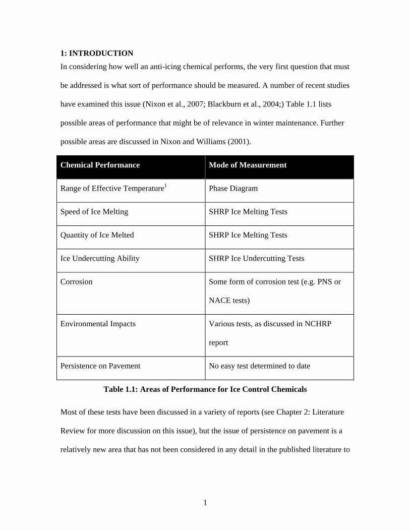
have examined this issue (Nixon et al., 2007; Blackburn et al., 2004;) Table 1.1 lists

possible areas of performance that might be of relevance in winter maintenance. Further

possible areas are discussed in Nixon and Williams (2001).

Chemical Performance Mode of Measurement

Range of Effective Temperature1 Phase Diagram

Speed of Ice Melting SHRP Ice Melting Tests

Quantity of Ice Melted SHRP Ice Melting Tests

Ice Undercutting Ability SHRP Ice Undercutting Tests

Corrosion Some form of corrosion test (e.g. PNS or

NACE tests)

Environmental Impacts Various tests, as discussed in NCHRP

report

Persistence on Pavement No easy test determined to date

Table 1.1: Areas of Performance for Ice Control Chemicals

Most of these tests have been discussed in a variety of reports (see Chapter 2: Literature

Review for more discussion on this issue), but the issue of persistence on pavement is a

relatively new area that has not been considered in any detail in the published literature to

2

date. It basically concerns how long a reasonable amount of chemical remains on the

traveled way under the effects of traffic, before becoming ineffective. It appears to be a

function of the stickiness or tackiness of the material applied, but also reflects how the

material behaves when it is placed on the pavement. For example, salt brine tends to dry

out after being placed on the pavement, and the dry residue may be swept away by

passing cars. Anecdotes suggest that brine, used as a frost prevention treatment, may last

about 2 to 4 days before a new application is required (absent any significant

precipitation). In contrast, there are reports of a calcium chloride based liquid (calcium

chloride mixed with a relatively small amount of beet juice, sold in the Pacific Northwest

under the trade name of GeoMelt™) that is sufficiently “sticky” that it remains effective

for periods of up to ten days when used in a frost prevention mode (again, absent any

precipitation). Clearly the persistence of a chemical and the longevity of that chemical’s

effectiveness would have a significant impact on the economics of using that chemical

versus another, less persistent chemical. Unfortunately, at present there does not appear

to be any consistent or suitably representative method of measuring this persistence.

Accordingly, while it should be a factor in any decision regarding the use of particular

chemicals, there is no way to incorporate this important factor into the models developed

in this study. Users of those models should be particularly aware of this drawback in the

models.

Perhaps the most widely used anti-icing and deicing chemical in the United States at

present is Sodium Chloride. It is readily available, is cheaper to buy than any other

deicing chemical and is very effective at melting snow and ice. Iowa uses about 190,000

1 Throughout this document the term “temperature” should be taken to indicate surface or pavement

3

tons of sodium chloride annually (this is a five year moving average from the Iowa DOT

website2). However, there are limits to its ability. A phase diagram for the Sodium

Chloride – water system shows that the eutectic temperature (the temperature below

which no ice can be melted by adding salt) is around –6° F (see e.g. Minsk, 1998).

However, in practice, sodium chloride becomes an ineffective deicing agent at higher

temperatures. Typically, salt is considered ineffective at between 15° and 20° F. Once

the temperature drops below these levels, then agencies have two possible choices: use

another chemical, or stop using chemicals altogether, and only plow and/or use abrasives.

Two other chlorides (Calcium Chloride and Magnesium Chloride) both can be used at

lower temperatures than Sodium Chloride, but both have some additional drawbacks,

especially with regard to cost and corrosiveness. There are some newer, organic

chemicals that have the ability to be effective at low temperatures (low in this case being

considered to be below the 15° F cut-off for salt use). In particular, Potassium Acetate

and Methyl Glucoside both have the ability to melt snow and ice at temperatures down to

around 0° F. However, both are extremely expensive. In practice in Iowa, chemical

usage is limited to Sodium Chloride and Calcium Chloride, although limited amounts of

other chemicals are used, mostly on an experimental basis.

However, there is concern that winter maintenance practice in Iowa may be using

Calcium Chloride in ways that are less than optimal. Iowa is typically rather cold in

winter. This suggests that there are a significant number of occasions when use of

Calcium Chloride might be more effective than use of Sodium Chloride. It’s also

temperature unless otherwise specified.

4

possible that a mix of the two chemicals might be a useful option to consider. The goal

of this project is to examine how well various mixes of the two chemicals (Sodium

Chloride and Calcium Chloride) perform over a range of temperatures. On that basis, a

cost/benefit comparison can be run which would indicate which “mix” should be used

under which conditions (primarily but not exclusively as a function of temperature).

Further, because anecdotal reports indicate that occasionally Calcium Chloride

applications can turn to “snot,” a range of mixes will be examined to determine whether

any particular mixes seem prone to such degradation.

2 http://www.dot.state.ia.us/dot_overview/transportationfacts_september2004.htm#Roads referenced on January 28, 2008.

5

2: LITERATURE SEARCH

The basic performance issue here relates to the phase diagrams of the Sodium Chloride –

Water and the Calcium Chloride – Water chemical systems. These are clearly well

established in the literature, and can be found in typical reference works as well as in

texts such as Minsk (1999) that are more focused on winter maintenance issues. Figure

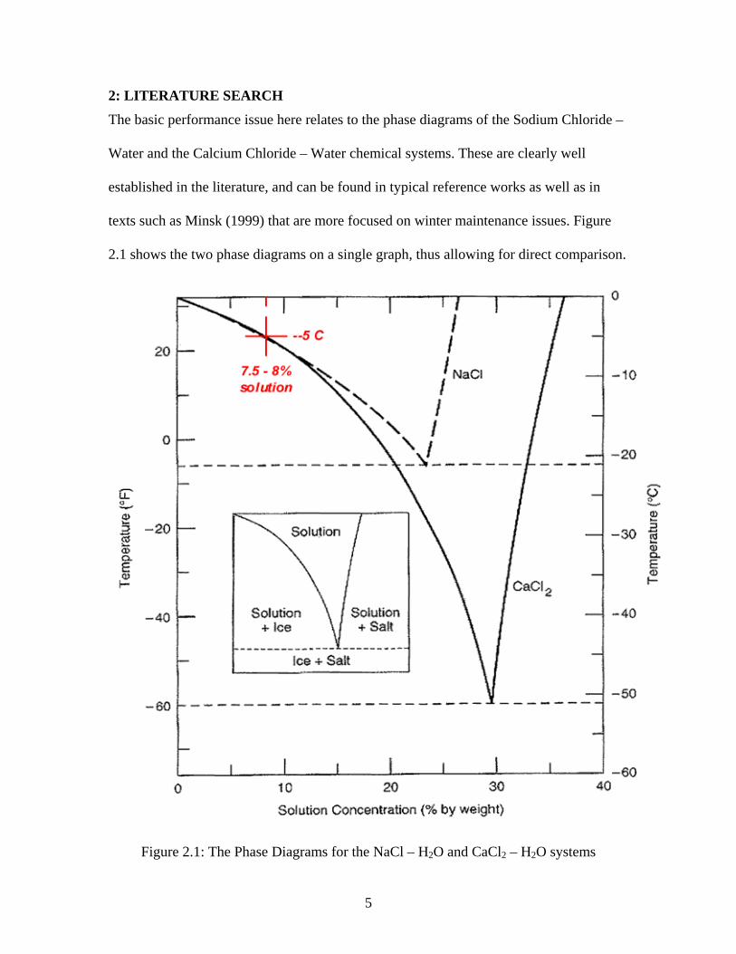
2.1 shows the two phase diagrams on a single graph, thus allowing for direct comparison.

Figure 2.1: The Phase Diagrams for the NaCl – H2O and CaCl2 – H2O systems

6

A number of points are apparent from Figure 2.1. First, at warmer temperatures (above

20° F) there is little difference between the melting curves for the two systems. Thus, as

shown by the red cross on the diagram, at -5° C (or 23° F) the percentage of either salt or

calcium chloride in a solution with water that will just begin to freeze is about 7.5 to 8%.

It is only when the temperature drops below 20° F that calcium chloride begins to

significantly out-perform sodium chloride.

Second, any phase diagram is an equilibrium based representation. That is, it properly

represents the situation when all phase changes have occurred. In winter maintenance,

this very rarely happens during a storm. Typically, the chemical applied to the road

surface is only melting a very thin layer of snow or ice. Should enough time pass, more

snow or ice will be melted, and the chemical will dilute out and start to freeze. Thus, we

should not expect that the phase diagram relates directly to performance in the field. As

one direct example, Figure 2.1 says nothing about how quickly the two chemicals act on

the pavement. Nonetheless, experience in the field clearly identifies calcium chloride as a

“hot” chemical that acts rapidly to melt snow and ice. The converse of this is that calcium

chloride will dilute out more quickly than sodium chloride. The scraping tests conducted

by Nixon (2003) confirm this comparative aspect of the two materials.

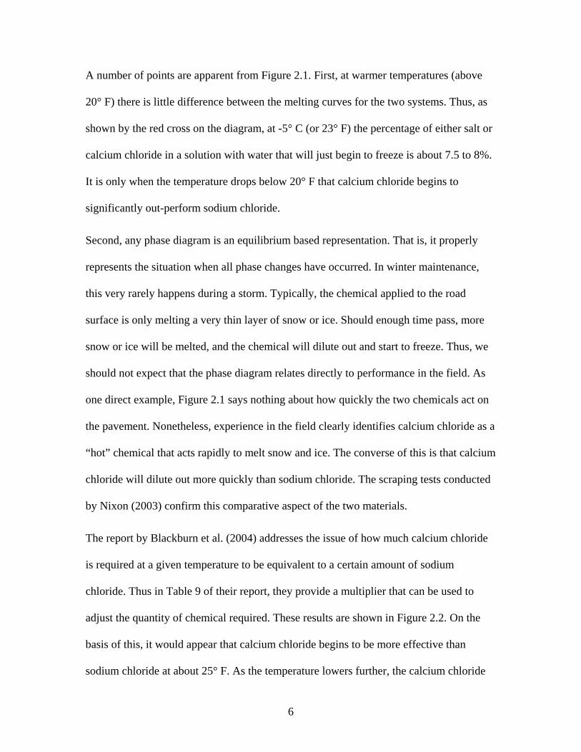
The report by Blackburn et al. (2004) addresses the issue of how much calcium chloride

is required at a given temperature to be equivalent to a certain amount of sodium

chloride. Thus in Table 9 of their report, they provide a multiplier that can be used to

adjust the quantity of chemical required. These results are shown in Figure 2.2. On the

basis of this, it would appear that calcium chloride begins to be more effective than

sodium chloride at about 25° F. As the temperature lowers further, the calcium chloride

7

becomes significantly more effective. This increased effectiveness is made more apparent

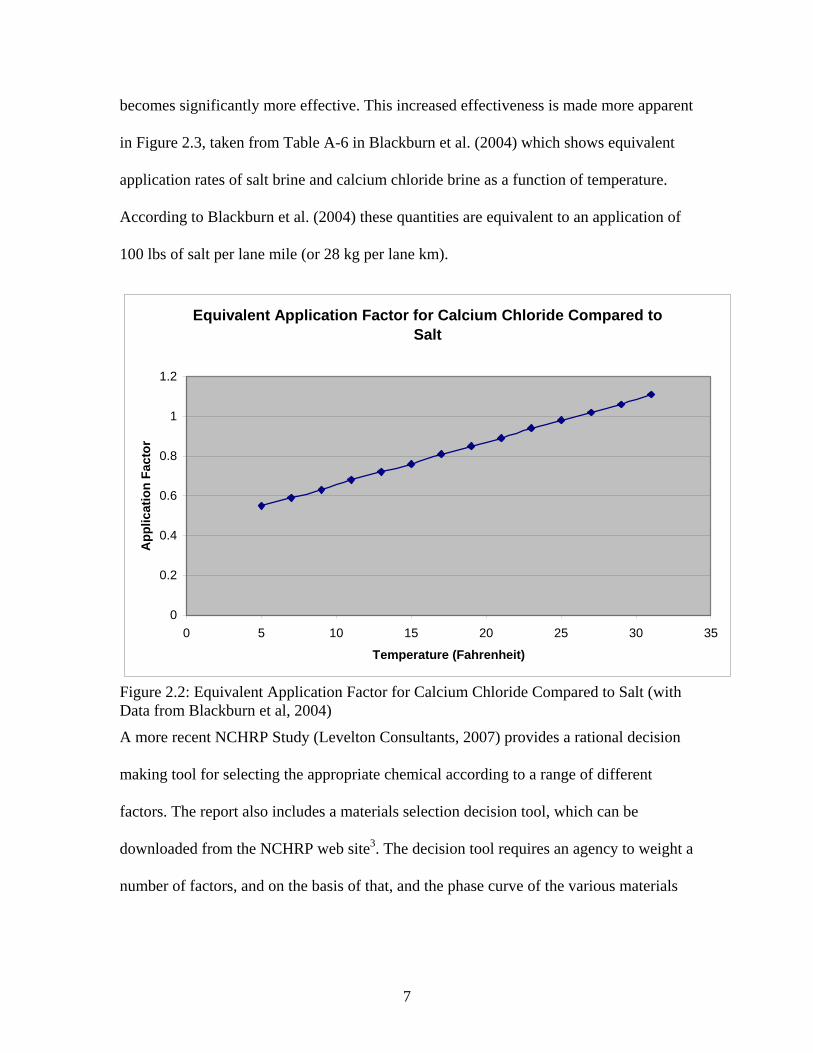
in Figure 2.3, taken from Table A-6 in Blackburn et al. (2004) which shows equivalent

application rates of salt brine and calcium chloride brine as a function of temperature.

According to Blackburn et al. (2004) these quantities are equivalent to an application of

100 lbs of salt per lane mile (or 28 kg per lane km).

Equivalent Application Factor for Calcium Chloride Compared to Salt

0

0.2

0.4

0.6

0.8

1

1.2

0 5 10 15 20 25 30 35

Temperature (Fahrenheit)

App

licat

ion

Fact

or

Figure 2.2: Equivalent Application Factor for Calcium Chloride Compared to Salt (with Data from Blackburn et al, 2004)

A more recent NCHRP Study (Levelton Consultants, 2007) provides a rational decision

making tool for selecting the appropriate chemical according to a range of different

factors. The report also includes a materials selection decision tool, which can be

downloaded from the NCHRP web site3. The decision tool requires an agency to weight a

number of factors, and on the basis of that, and the phase curve of the various materials

8

under consideration (primarily the five chemicals identified in Chapter 1 above) the tool

generates a curve showing the score for each chemical as a function of temperature. The

tool can use data from other chemicals as needed, on the basis of phase curve for the

other chemicals. However, the tool does not have any feature allowing a mix of

chemicals to be examined, unless a phase curve exists for that mix.

Comparative Quantities of Brine Required as a Function of Temperature

0

20

40

60

80

100

120

140

160

180

0 5 10 15 20 25 30 35


Gal

lons

of B

rine

per L

ane

Mile

Sodium Chloride BrineCalcium Chloride

Figure 2.3: Comparative Quantities of Brine Required as a Function of Temperature (with Data from Blackburn et al, 2004)

Two agencies have been making use of mixtures of sodium chloride and calcium chloride

(together with a beet juice based additive): the City of West Des Moines, Iowa, and

McHenry County, Illinois. A number of presentations on their methods and their results

are available on the APWA web site4. Their general experience has been that the mixture

3 The tool can be downloaded from http://www.trb.org/TRBNet/ProjectDisplay.asp?ProjectID=883, accessed on January 30, 2008. 4 Available at http://www.apwa.net/Meetings/Snow/2007/handouts/ accessed on February 1, 2008.

9

they use, which they call Supermix, works better than straight salt brine in the winter

weather conditions they face regularly. Most importantly, the blend remains effective for

much longer than typical salt brine. This is an important point operationally, and should

definitely be considered in any chemical selection decisions. A representative of one of

the two agencies noted above stated explicitly that they use the mix not for improved low

temperature performance but strictly for enhanced persistence (DeVries, Personal

Communication, 2007). However, as indicated above, currently no standard test exists to

measure the effective longevity of an ice control chemical on the pavement. The

development of such a test was beyond the scope of this project, but may need to be

considered in the future should this become a critical operational concern. It is perhaps

worth noting that a number of other agencies have expressed considerable interest in the

chemical mixing approach (again, see the APWA web site for details) and many agencies

(including International agencies) have visited either West Des Moines or McHenry

County to learn more.

To summarize the current literature as it pertains to the use of chemical mixtures as ice

control products, there is little published that is of direct relevance in this regard. While

tools are available to rate and evaluate ice control chemicals, in order to use these for

chemical mixtures, a new phase curve would have to be developed for each such mixture.

This is by no means impossible, but it suggests a great deal of labor to discover that a

mixture may not, after all, be particularly effective.

10

3: DETERMINING PROPERTIES OF THE MIXTURES

It was determined that two properties would be considered in constructing the economic

model. These two properties were the ice melting capability, and the freezing point. The

first step in gaining sufficient information to develop the model was to determine these

capabilities for the two “baseline” products: salt brine and calcium chloride brine.

3.1 Baseline Testing

There are two aspects to the baseline testing: the ice melting capacity, and the freezing

point of the brines. The baseline tests and results are described in this section.

Baseline testing of ice melting capacity was conducted using the SHRP H-332 Report,

entitled “Handbook of Test Methods for Evaluating Chemical Deicers” published in

1992. The use of the tests is described more fully in Nixon et al. (2007). The test used

was H-205.2 Test Method for Ice Melting of Liquid deicing Chemicals. The two

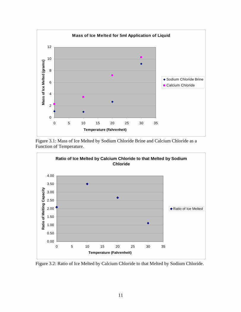
chemicals were tested at 30°, 20°, 10° and 0° F. Figure 3.1 shows how much ice was

melted (measured in grams) by the application of 5 ml of ice control liquid after a period

of one hour.

As expected, at 30° F there is relatively little difference between the two chemicals. The

difference is much more pronounced at lower temperatures. The difference in chemicals

is more clearly seen if the ratio of ice melted by calcium chloride to ice melted by sodium

chloride brine is plotted as a function of temperature, as shown in Figure 3.2.

11

Mass of Ice Melted for 5ml Application of Liquid

0

2

4

6

8

10

12

0 5 10 15 20 25 30 35


Mas

s of

Ice

Mel

ted

(gra

ms)

Sodium Chloride Brine

Calcium Chloride

Figure 3.1: Mass of Ice Melted by Sodium Chloride Brine and Calcium Chloride as a Function of Temperature.

Ratio of Ice Melted by Calcium Chloride to that Melted by Sodium Chloride

0.00

0.50

1.00

1.50

2.00

2.50

3.00

3.50

4.00

0 5 10 15 20 25 30 35


Rat

io o

f Mel

ting

Cap

acity

Ratio of Ice Melted

Figure 3.2: Ratio of Ice Melted by Calcium Chloride to that Melted by Sodium Chloride.

12

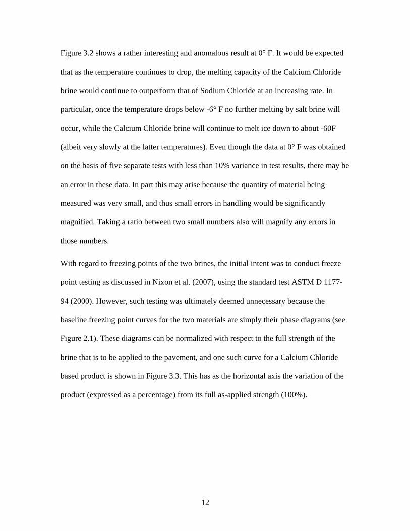
Figure 3.2 shows a rather interesting and anomalous result at 0° F. It would be expected

that as the temperature continues to drop, the melting capacity of the Calcium Chloride

brine would continue to outperform that of Sodium Chloride at an increasing rate. In

particular, once the temperature drops below -6° F no further melting by salt brine will

occur, while the Calcium Chloride brine will continue to melt ice down to about -60F

(albeit very slowly at the latter temperatures). Even though the data at 0° F was obtained

on the basis of five separate tests with less than 10% variance in test results, there may be

an error in these data. In part this may arise because the quantity of material being

measured was very small, and thus small errors in handling would be significantly

magnified. Taking a ratio between two small numbers also will magnify any errors in

those numbers.

With regard to freezing points of the two brines, the initial intent was to conduct freeze

point testing as discussed in Nixon et al. (2007), using the standard test ASTM D 1177-

94 (2000). However, such testing was ultimately deemed unnecessary because the

baseline freezing point curves for the two materials are simply their phase diagrams (see

Figure 2.1). These diagrams can be normalized with respect to the full strength of the

brine that is to be applied to the pavement, and one such curve for a Calcium Chloride

based product is shown in Figure 3.3. This has as the horizontal axis the variation of the

product (expressed as a percentage) from its full as-applied strength (100%).

13

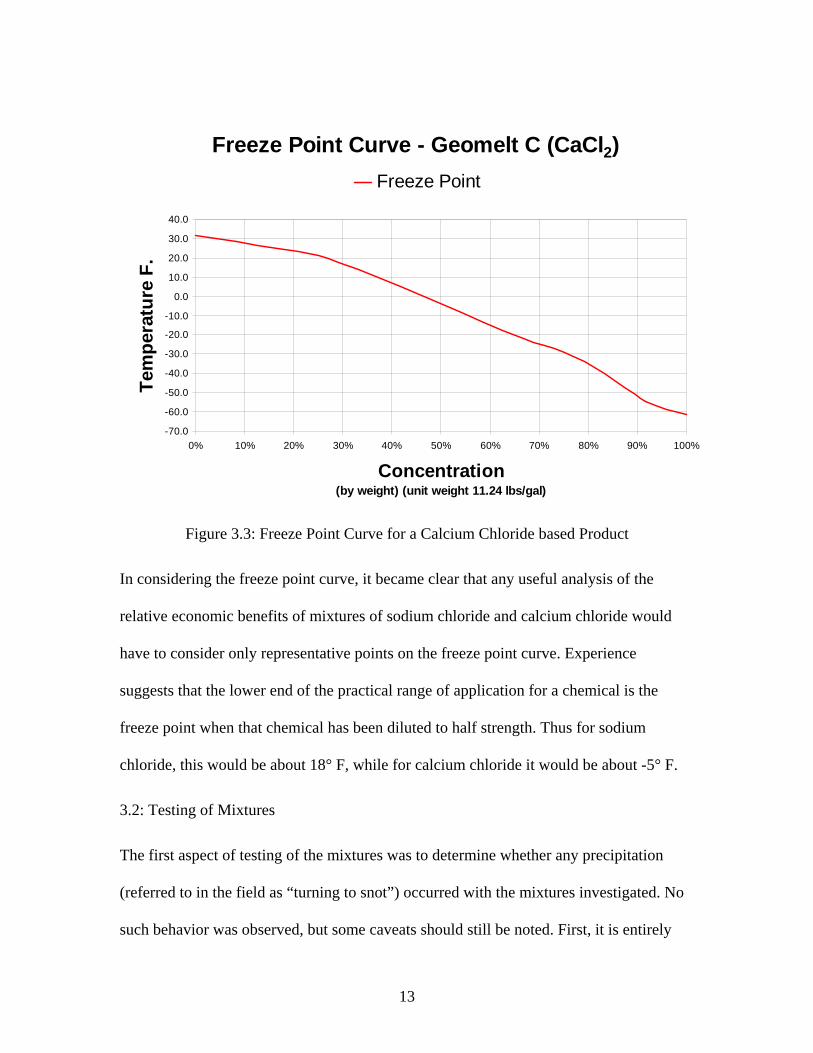
Figure 3.3: Freeze Point Curve for a Calcium Chloride based Product

In considering the freeze point curve, it became clear that any useful analysis of the

relative economic benefits of mixtures of sodium chloride and calcium chloride would

have to consider only representative points on the freeze point curve. Experience

suggests that the lower end of the practical range of application for a chemical is the

freeze point when that chemical has been diluted to half strength. Thus for sodium

chloride, this would be about 18° F, while for calcium chloride it would be about -5° F.

3.2: Testing of Mixtures

The first aspect of testing of the mixtures was to determine whether any precipitation

(referred to in the field as “turning to snot”) occurred with the mixtures investigated. No

such behavior was observed, but some caveats should still be noted. First, it is entirely

Freeze Point Curve - Geomelt C (CaCl2)

-70.0

-60.0

-50.0

-40.0

-30.0

-20.0

-10.0

0.0

10.0

20.0

30.0

40.0

0% 10% 20% 30% 40% 50% 60% 70% 80% 90% 100%

Concentration(by weight) (unit weight 11.24 lbs/gal)

Tem

pera

ture

F.

Freeze Point

14

possible that how the two chemicals are mixed may have an impact on whether any

precipitation occurs. In our tests, calcium chloride was always added to salt brine, in

general in small quantities and relatively slowly. Other methods of mixing may result in

problems occurring, although it should be noted that the mixing methods used at West

Des Moines and McHenry County have not shown any evidence of precipitation either.

Second, many calcium chloride brines used in winter maintenance are in fact calcium

chloride plus, where the “plus” may indicate a range of additives most often intended as

corrosion preventatives. Only one type of calcium chloride brine was used in these tests,

from the Davenport Garage of the Iowa DOT. Whether other additives to the calcium

chloride may cause some sort of precipitation event is not known and has not been

examined as part of this study.

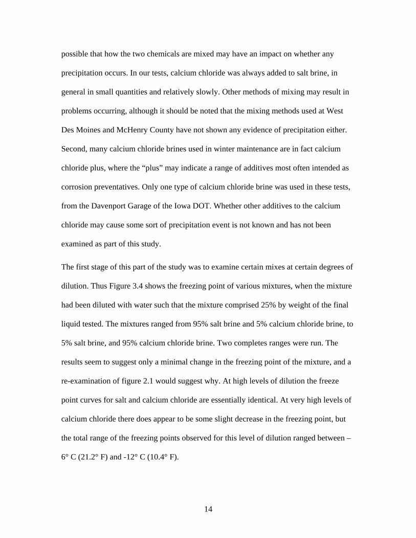
The first stage of this part of the study was to examine certain mixes at certain degrees of

dilution. Thus Figure 3.4 shows the freezing point of various mixtures, when the mixture

had been diluted with water such that the mixture comprised 25% by weight of the final

liquid tested. The mixtures ranged from 95% salt brine and 5% calcium chloride brine, to

5% salt brine, and 95% calcium chloride brine. Two completes ranges were run. The

results seem to suggest only a minimal change in the freezing point of the mixture, and a

re-examination of figure 2.1 would suggest why. At high levels of dilution the freeze

point curves for salt and calcium chloride are essentially identical. At very high levels of

calcium chloride there does appear to be some slight decrease in the freezing point, but

the total range of the freezing points observed for this level of dilution ranged between –

6° C (21.2° F) and -12° C (10.4° F).

15

75% Diluted Mixture Freezing Point

-14

-12

-10

-8

-6

-4

-2

00 20 40 60 80 100

%age of Salt in Original Mixture

Tem

pera

ture

(Cen

tigra

de)

FP 1FP 2FP Ave

Figure 3.4: Variation of Freezing Point of Salt-Calcium Chloride Mixtures when Diluted with 75% water.

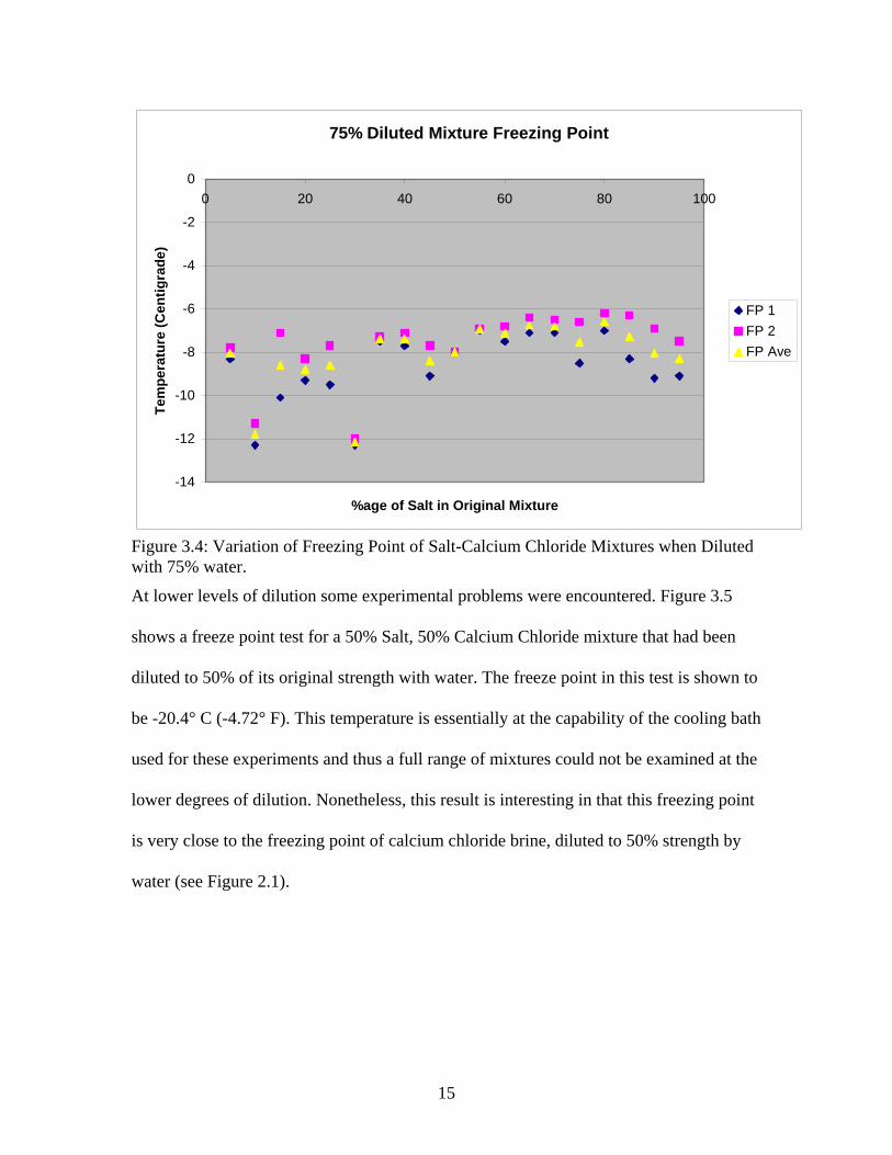
At lower levels of dilution some experimental problems were encountered. Figure 3.5

shows a freeze point test for a 50% Salt, 50% Calcium Chloride mixture that had been

diluted to 50% of its original strength with water. The freeze point in this test is shown to

be -20.4° C (-4.72° F). This temperature is essentially at the capability of the cooling bath

used for these experiments and thus a full range of mixtures could not be examined at the

lower degrees of dilution. Nonetheless, this result is interesting in that this freezing point

is very close to the freezing point of calcium chloride brine, diluted to 50% strength by

water (see Figure 2.1).

16

Figure 3.5: Freeze Point experiment Results for 50% Salt, 50% Calcium Chloride mixture that had been diluted to 50% of its original strength with water

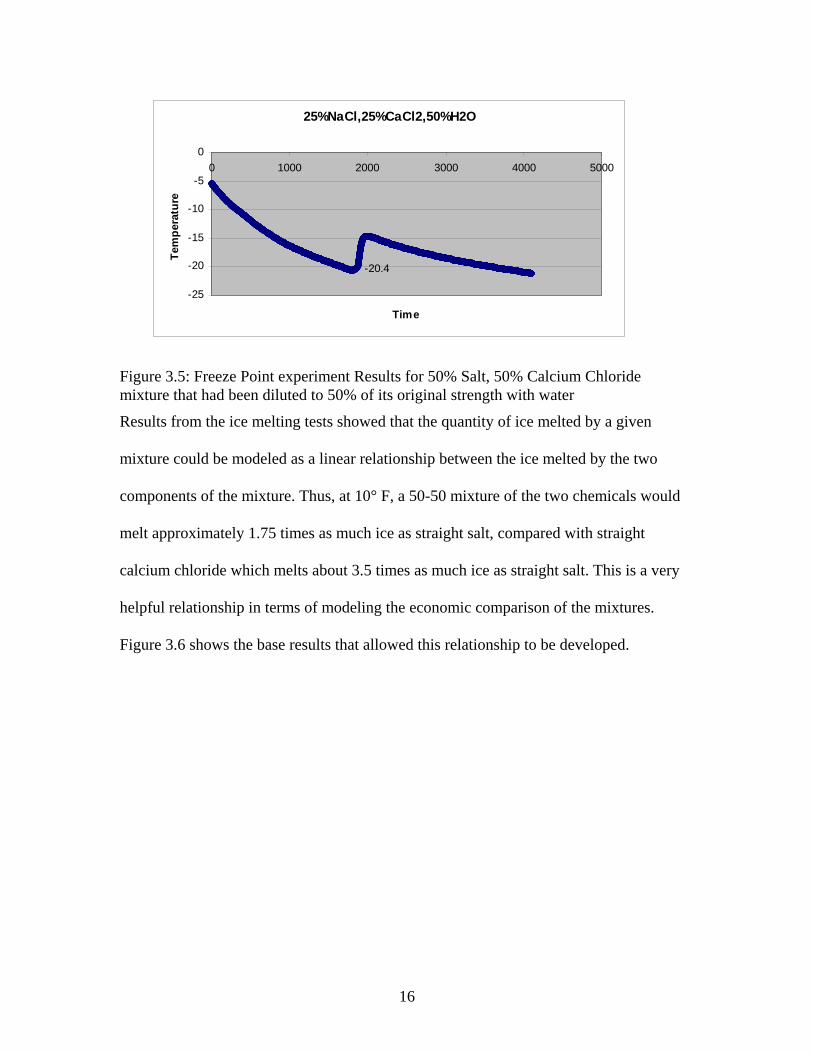
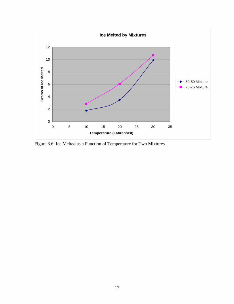
Results from the ice melting tests showed that the quantity of ice melted by a given

mixture could be modeled as a linear relationship between the ice melted by the two

components of the mixture. Thus, at 10° F, a 50-50 mixture of the two chemicals would

melt approximately 1.75 times as much ice as straight salt, compared with straight

calcium chloride which melts about 3.5 times as much ice as straight salt. This is a very

helpful relationship in terms of modeling the economic comparison of the mixtures.

Figure 3.6 shows the base results that allowed this relationship to be developed.

25%NaCl,25%CaCl2,50%H2O

-20.4

-25

-20

-15

-10

-5

00 1000 2000 3000 4000 5000

Time

Tem

pera

ture

17

Ice Melted by Mixtures

0

2

4

6

8

10

12

0 5 10 15 20 25 30 35


Gra

ms

of Ic

e M

elte

d

50-50 Mixture25-75 Mixture

Figure 3.6: Ice Melted as a Function of Temperature for Two Mixtures

18

4: MODEL DEVELOPMENT

4.1: Initial Requirements

On the basis of the experimental results discussed in chapter 3 above, it is reasonable to

model the behavior of mixtures of sodium chloride and calcium chloride brines with a

linear model, directly proportional to the percentage of the mixture. While the

relationship may not actually be linear, the data do not provide enough information to

justify a more complex model.

While there are a number of things that could be used to model the ice melting

performance of the mixture, the process by which ice is melted on the pavement is not yet

fully clear (see Nixon et al., 2007). The quantity of ice or snow that can be melted by a

reasonable application of salt is very small, as the following calculations show. If the

phase diagram for salt (sodium chloride) is considered (see Figure 2.1) we can see that at

a temperature of 23° F, a salt-water mixture will begin to freeze when the mixture

comprises about 7.5% salt by weight. If we take a reasonably high application rate of 300

lbs per lane mile, we can use the phase diagram to calculate how much moisture will

dilute this application to the point at which it starts to freeze. The first step in the

calculation is a simple evaluation of how much water must be added to the 300 lbs of salt

to create a 7.5% solution:

(4.1)

This quantity of water can now be converted to a depth of water across the lane

mile over which the 300 lbs of salt is spread:

( ) water/milemilelbsW lbs 3700/300%5.7%5.92 ==

19

(4.2)

Given this result, it is clear that relatively little snow or ice needs to be melted. One way

of modeling mixtures is to ask how much of a certain mixture is needed if a certain

quantity of ice is to be melted. Clearly, finding this involves a combination of using the

phase diagram, and using application quantities that have proven effective in the field. In

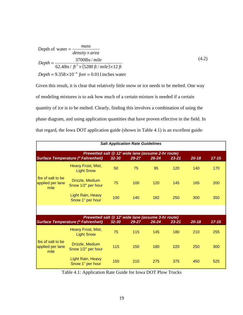
that regard, the Iowa DOT application guide (shown in Table 4.1) is an excellent guide:

32-30 29-27 26-24 23-21 20-18 17-15

32-30 29-27 26-24 23-21 20-18 17-15

100

182

170

200

Surface Temperature (º Fahrenheit)

lbs of salt to be applied per lane

mile

Heavy Frost, Mist, Light Snow

Drizzle, Medium Snow 1/2" per hour

120 140

120

220 250 300

350300250

180 210 255

Salt Application Rate Guidelines

165145

Light Rain, Heavy Snow 1" per hour

50 75 95

75

100 140

115 150 180

Surface Temperature (º Fahrenheit)

lbs of salt to be applied per lane

mile

Heavy Frost, Mist, Light Snow 75 115 145

375 450 525

Prewetted salt @ 12' wide lane (assume 2-hr route)

Prewetted salt @ 12' wide lane (assume 3-hr route)

Light Rain, Heavy Snow 1" per hour 150 210 275

Drizzle, Medium Snow 1/2" per hour

Table 4.1: Application Rate Guide for Iowa DOT Plow Trucks

( ) waterinches 011.010358.912/5280/4.62

/3700

waterofDepth

4

3

=×=××

=

×=

− feetDepthftmileftftlbs

milelbsDepth

areadensitymass

20

Using this table, we can take a condition that is relatively common, and use it and

equations 4.1 and 4.2 to determine how much of any given mixture is required at any

given temperature. If we consider a two hour cycle time, with a temperature of 23° F and

medium snow at ½ inch per hour, we get an application rate of 145 lb per lane mile. This

translates into melting approximately 0.006 inches of ice. Clearly other approaches could

be used, but this has the benefit of simplicity, and a clear link to current practice which

experience has shown to be effective.

4.2 Linear Representation of the Mixtures

As indicated above, the performance of mixtures of the two brines will be based on a

linear relationship between them. The approach to this will be to consider temperatures

between 32° and -5° F. Since the low end of the effective temperature range for calcium

chloride is generally taken to be close to -5° F, there is no value in going to lower

temperatures, and of course, below -6.02° F, sodium chloride will not melt any ice at all.

For a given temperature, the percentage of each brine at which freezing just begins

(specifically, the percentage at which the liquidus line is crossed) will be expressed as a

percentage of the eutectic concentration. Thus, if at 23° F, sodium chloride just begins to

freeze (crosses the liquidus line) then this is at a concentration of 7.5% salt by weight

(see figure 2.1 and equations 4.1 and 4.2 above). Given that the eutectic concentration for

sodium chloride in the sodium chloride-water system is approximately 23%, then the

sodium chloride brine at 23° F will begin to freeze at 32.6% (7.5/23) of its eutectic

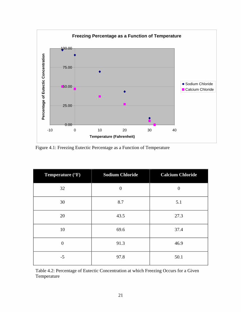
concentration. Figure 4.1 shows this relationship for both sodium chloride and calcium

chloride brines. Table 4.2 provides the values in tabular form.

21

Freezing Percentage as a Function of Temperature

0.00

25.00

50.00

75.00

100.00

-10 0 10 20 30 40


Perc

enta

ge o

f Eut

ectic

Con

cent

ratio

n

Sodium ChlorideCalcium Chloride

Figure 4.1: Freezing Eutectic Percentage as a Function of Temperature

Temperature (°F) Sodium Chloride Calcium Chloride

32 0 0

30 8.7 5.1

20 43.5 27.3

10 69.6 37.4

0 91.3 46.9

-5 97.8 50.1

Table 4.2: Percentage of Eutectic Concentration at which Freezing Occurs for a Given Temperature

22

If information is required for a temperature between the values listed in the table, linear

interpolation will provide appropriate values. Thus for a temperature of 8° F, the

percentage of eutectic concentration (P) at which freezing occurs is given as:

( )010

810100108 TT

TTPPPP

−−

−+= 4.1

For Sodium Chloride this is 74.0% and for Calcium Chloride this is 39.3%. If a mixture

of the two is then specified (e.g x% NaCl and y% CaCl2, where x+y = 100), then the final

percentage of eutectic or applied concentration at which freezing will occur (Pmix) is

given as:

100100288 CaClNaCl

mixyPxP

P += 4.2

So in a mix with 80% sodium chloride and 20% calcium chloride, the final percentage of

applied concentration would be 67.1%.

4.3 Determining the Quantity of the Mixture Required

Taking, from above, the goal of melting a water equivalent of 0.006” of ice or snow, the

next step is to determine how much of the mixture is required to achieve this goal. A

preliminary step is determining the weight of water (Ww) that a 0.006” layer on the road

surface equals per lane mile. This quantity is found as:

DensityVolumeWeight ×= 4.3

where volume is expressed in cubic feet, and density in pounds per cubic foot. For the

0.006” layer thickness this gives:

23

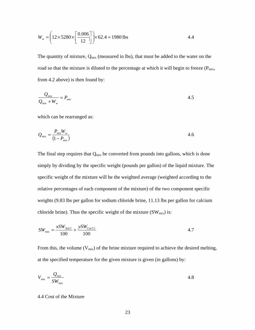
lbs 19804.6212006.0528012 =×⎟⎟

⎠

⎞⎜⎜⎝

⎛⎥⎦⎤

⎢⎣⎡××=wW 4.4

The quantity of mixture, Qmix (measured in lbs), that must be added to the water on the

road so that the mixture is diluted to the percentage at which it will begin to freeze (Pmix,

from 4.2 above) is then found by:

mixwmix

mix PWQ

Q=

+ 4.5

which can be rearranged as:

( )mix

wmixmix P

WPQ

−=

1 4.6

The final step requires that Qmix be converted from pounds into gallons, which is done

simply by dividing by the specific weight (pounds per gallon) of the liquid mixture. The

specific weight of the mixture will be the weighted average (weighted according to the

relative percentages of each component of the mixture) of the two component specific

weights (9.83 lbs per gallon for sodium chloride brine, 11.13 lbs per gallon for calcium

chloride brine). Thus the specific weight of the mixture (SWmix) is:

1001002CaClNaCl

mixySWxSW

SW += 4.7

From this, the volume (Vmix) of the brine mixture required to achieve the desired melting,

at the specified temperature for the given mixture is given (in gallons) by:

mix

mixmix SW

QV = 4.8

4.4 Cost of the Mixture

24

One goal of this project was to be able to compare costs of possible mixtures with costs

of straight brine, over a range of temperatures. To do this, three steps are needed. First, at

a given temperature, determine how much sodium chloride brine would be required to

achieve the desired amount of melting. This can be done by using equations 4.1 through

4.8 with the percentage of sodium chloride brine at 100%. Second, having chosen a

mixture to investigate, the quantity of the mixed brine at the given temperature is again

found, using equations 4.1 through 4.8. Finally, costs for the two brine quantities are

calculated, using unit costs assigned as appropriate. The costs for the mixture can then be

compared with the costs for the salt brine.

These costs can be calculated relatively simply, using a spreadsheet, and this has been

done and is reported in Chapter 5 below. The inputs required for the spreadsheet

calculations are the costs of sodium chloride brine and calcium chloride brine, and the

percentage of each brine in the mixture to be investigated.

As discussed above, it should be noted that this comparison rests upon the need for a

chemical application to melt a given, specified, quantity of ice or snow (0.006” inch of

water equivalent). To the extent that this models ice melting performance, this approach

will give a reasonable answer. This approach does not address other performance issues,

such as persistence of chemical on the road. These other aspects may in certain

circumstances be a great deal more important than ice melting performance.

25

5: MODEL RESULTS

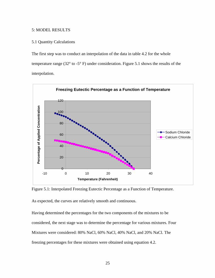
5.1 Quantity Calculations

The first step was to conduct an interpolation of the data in table 4.2 for the whole

temperature range (32° to -5° F) under consideration. Figure 5.1 shows the results of the

interpolation.

Freezing Eutectic Percentage as a Function of Temperature

0

20

40

60

80

100

120

-10 0 10 20 30 40


Perc

enta

ge o

f App

lied

Con

cent

ratio

n

Sodium ChlorideCalcium Chloride

Figure 5.1: Interpolated Freezing Eutectic Percentage as a Function of Temperature.

As expected, the curves are relatively smooth and continuous.

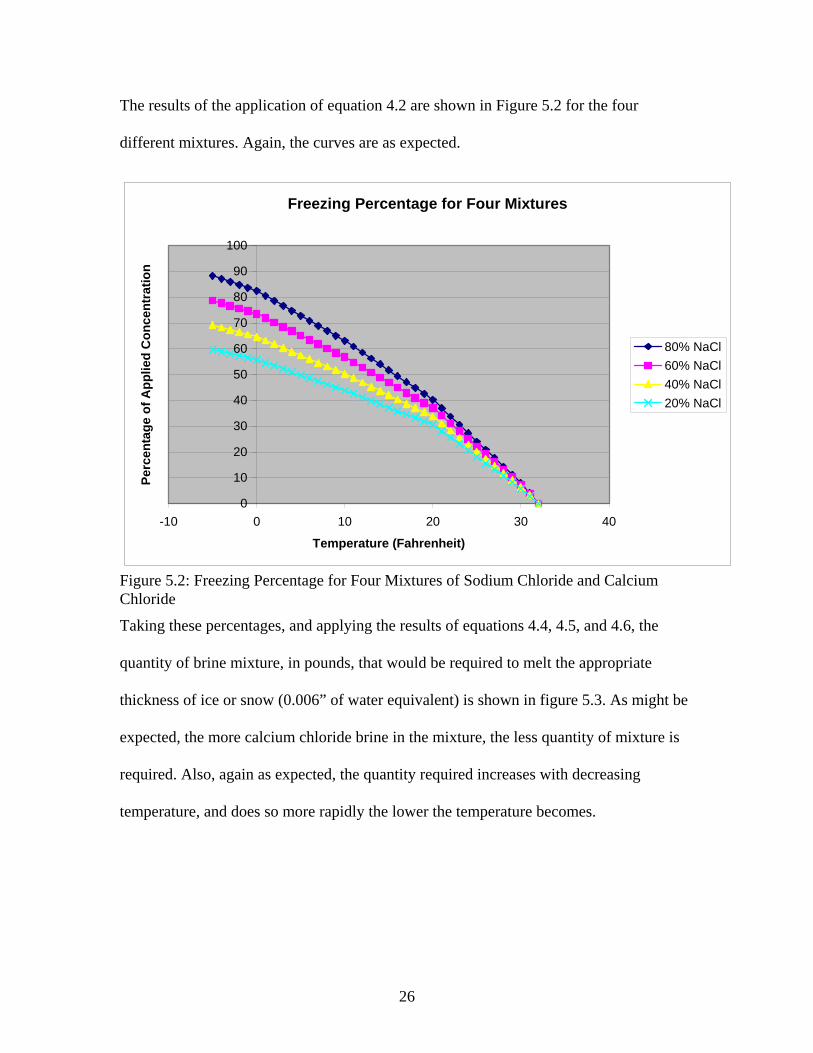
Having determined the percentages for the two components of the mixtures to be

considered, the next stage was to determine the percentage for various mixtures. Four

Mixtures were considered: 80% NaCl, 60% NaCl, 40% NaCl, and 20% NaCl. The

freezing percentages for these mixtures were obtained using equation 4.2.

26

The results of the application of equation 4.2 are shown in Figure 5.2 for the four

different mixtures. Again, the curves are as expected.

Freezing Percentage for Four Mixtures

0

10

20

30

40

50

60

70

80

90

100

-10 0 10 20 30 40


Perc

enta

ge o

f App

lied

Con

cent

ratio

n

80% NaCl60% NaCl40% NaCl20% NaCl

Figure 5.2: Freezing Percentage for Four Mixtures of Sodium Chloride and Calcium Chloride

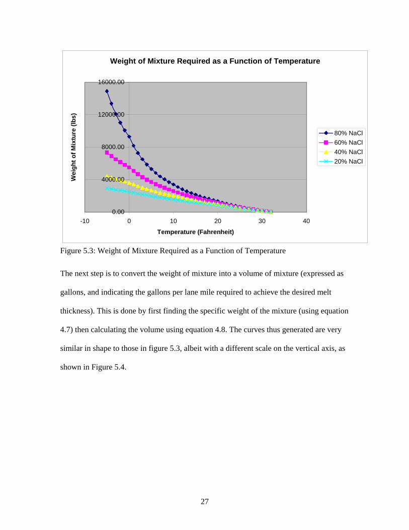
Taking these percentages, and applying the results of equations 4.4, 4.5, and 4.6, the

quantity of brine mixture, in pounds, that would be required to melt the appropriate

thickness of ice or snow (0.006” of water equivalent) is shown in figure 5.3. As might be

expected, the more calcium chloride brine in the mixture, the less quantity of mixture is

required. Also, again as expected, the quantity required increases with decreasing

temperature, and does so more rapidly the lower the temperature becomes.

27

Weight of Mixture Required as a Function of Temperature

0.00

4000.00

8000.00

12000.00

16000.00

-10 0 10 20 30 40


Wei

ght o

f Mix

ture

(lbs

)


Figure 5.3: Weight of Mixture Required as a Function of Temperature

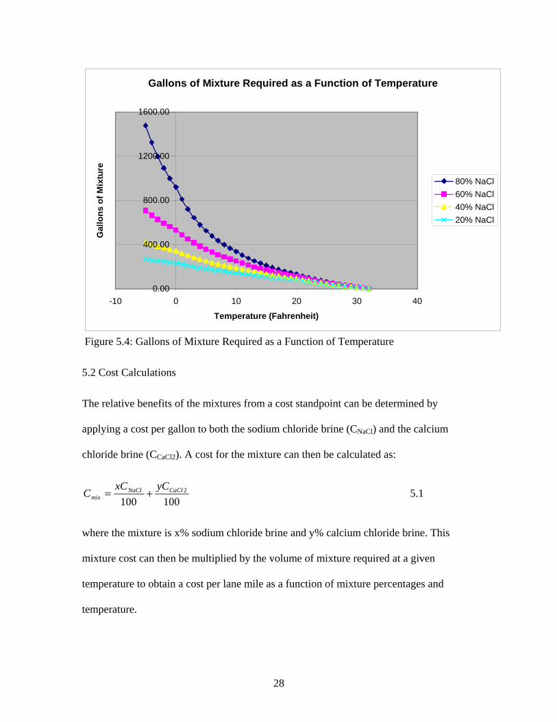
The next step is to convert the weight of mixture into a volume of mixture (expressed as

gallons, and indicating the gallons per lane mile required to achieve the desired melt

thickness). This is done by first finding the specific weight of the mixture (using equation

4.7) then calculating the volume using equation 4.8. The curves thus generated are very

similar in shape to those in figure 5.3, albeit with a different scale on the vertical axis, as

shown in Figure 5.4.

28

Gallons of Mixture Required as a Function of Temperature

0.00

400.00

800.00

1200.00

1600.00

-10 0 10 20 30 40


Gal

lons

of M

ixtu

re


Figure 5.4: Gallons of Mixture Required as a Function of Temperature

5.2 Cost Calculations

The relative benefits of the mixtures from a cost standpoint can be determined by

applying a cost per gallon to both the sodium chloride brine (CNaCl) and the calcium

chloride brine (CCaCl2). A cost for the mixture can then be calculated as:

1001002CaClNaCl

mixyCxC

C += 5.1

where the mixture is x% sodium chloride brine and y% calcium chloride brine. This

mixture cost can then be multiplied by the volume of mixture required at a given

temperature to obtain a cost per lane mile as a function of mixture percentages and

temperature.

29

Clearly the results of this calculation are extremely dependent upon the relative costs

assigned for a gallon of sodium chloride brine and a gallon of calcium chloride brine.

Table 5.1 shows the combinations of costs that were considered in this study.

Sodium Chloride Brine Cost per Gallon Calcium Chloride Brine Cost per Gallon

$0.05 $0.80

$0.05 $1.00

$0.05 $1.20

$0.10 $0.80

$0.10 $1.00

$0.10 $1.20

Table 5.1: Cost Combinations for the Two Brines

In considering these six costs combinations, comparisons will be made between applying

straight salt and two different mixtures, the first with 80% NaCl, the second with 20%

NaCl. This brackets the range of possible mixtures and provides insights into what sort of

mixtures are likely to be most beneficial under which conditions.

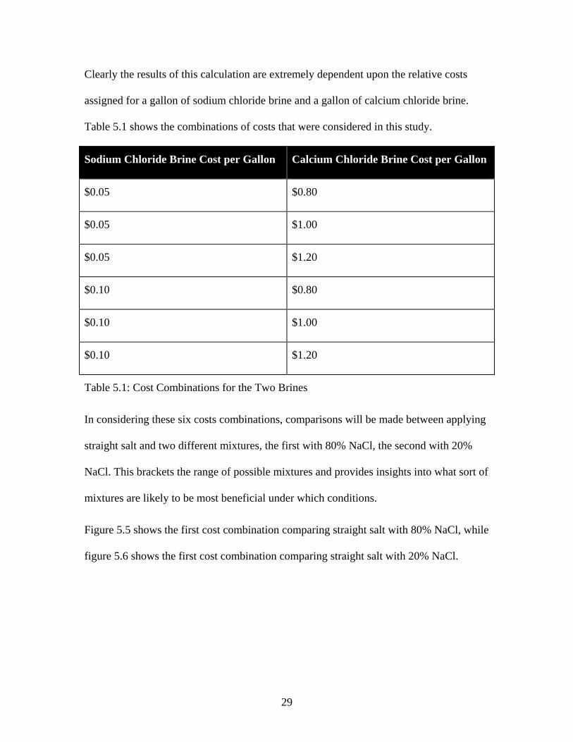
Figure 5.5 shows the first cost combination comparing straight salt with 80% NaCl, while

figure 5.6 shows the first cost combination comparing straight salt with 20% NaCl.

30

Cost as a Function of Temperature (Salt $0.05, Calcium $0.80)

$0.00

$100.00

$200.00

$300.00

$400.00

$500.00

-10 0 10 20 30 40


Cos

t per

Lan

e M

ile

80% NaClsalt cost

Figure 5.5: Cost Comparison, 80% NaCl, Salt $0.05, Calcium Chloride $0.80


$0.00

$100.00

$200.00

$300.00

$400.00

$500.00

-10 0 10 20 30 40


Cos

t per

Lan

e M

ile

20% NaClsalt cost

Figure 5.6: Cost Comparison, 20% NaCl, Salt $0.05, Calcium Chloride $0.80

31

It is of interest to note that the 80% NaCl mixture becomes more economical at a

temperature of -4° F, while the 20% NaCl mixture becomes more economical at a

temperature of -2° F. Operationally, there is little difference between these two

“crossover” temperatures.

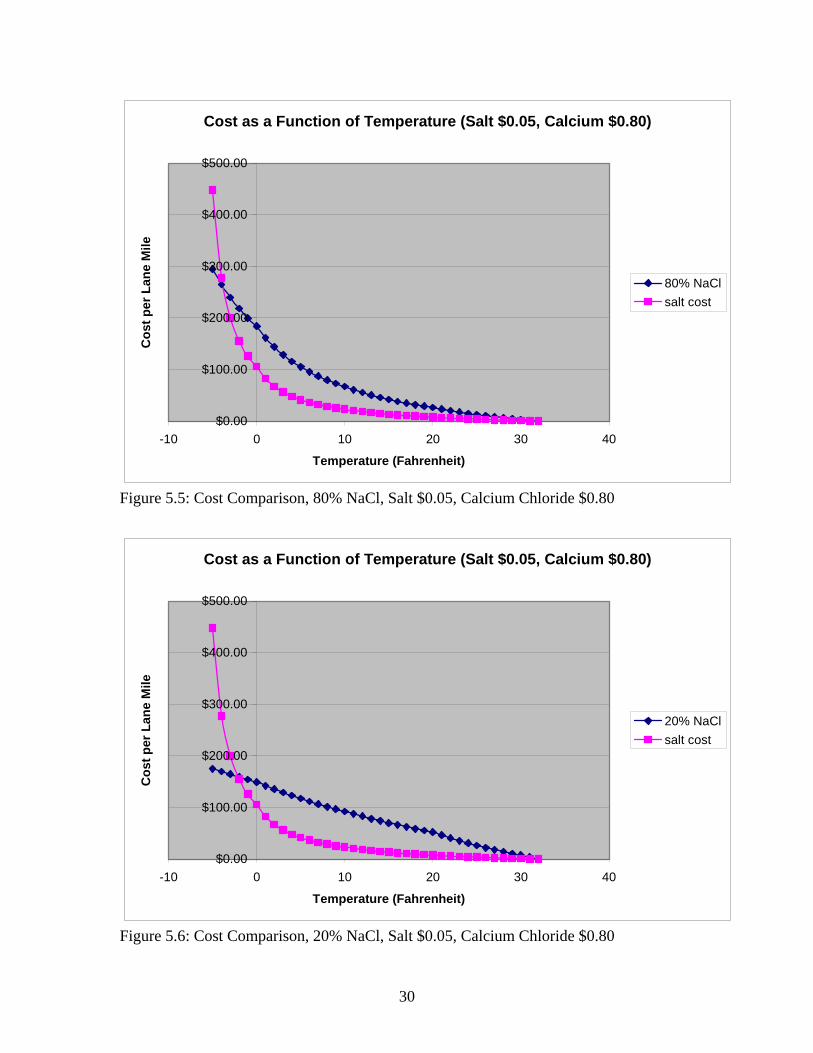
For the next cost combination (salt $0.05, and calcium chloride $1.00) the economic

crossover points occur at even lower temperatures, as shown in figure 5.7. Now the 80%

mixture is only economical at -5° F and the 20% mixture is economical at -3° F.


$0.00

$100.00

$200.00

$300.00

$400.00

$500.00

-10 0 10 20 30 40


Cos

t per

Lan

e M

ile

80% NaCl20% NaClsalt cost

Figure 5.7: Cost Comparison, 20% NaCl and 80% NaCl Salt $0.05, Calcium Chloride $1.00

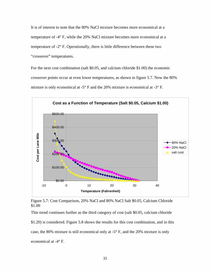
This trend continues further as the third category of cost (salt $0.05, calcium chloride

$1.20) is considered. Figure 5.8 shows the results for this cost combination, and in this

case, the 80% mixture is still economical only at -5° F, and the 20% mixture is only

economical at -4° F.

32


$0.00

$100.00

$200.00

$300.00

$400.00

$500.00

-10 0 10 20 30 40


Cos

t per

Lan

e M

ile



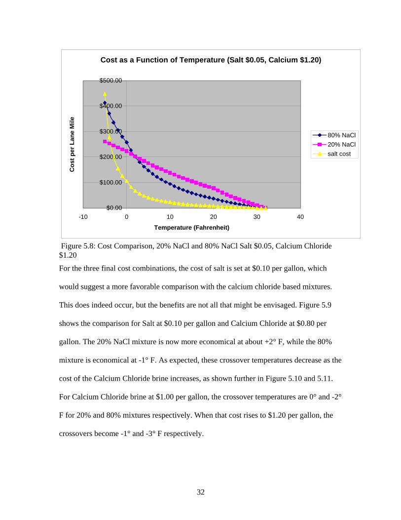
For the three final cost combinations, the cost of salt is set at $0.10 per gallon, which

would suggest a more favorable comparison with the calcium chloride based mixtures.

This does indeed occur, but the benefits are not all that might be envisaged. Figure 5.9

shows the comparison for Salt at $0.10 per gallon and Calcium Chloride at $0.80 per

gallon. The 20% NaCl mixture is now more economical at about +2° F, while the 80%

mixture is economical at -1° F. As expected, these crossover temperatures decrease as the

cost of the Calcium Chloride brine increases, as shown further in Figure 5.10 and 5.11.

For Calcium Chloride brine at $1.00 per gallon, the crossover temperatures are 0° and -2°

F for 20% and 80% mixtures respectively. When that cost rises to $1.20 per gallon, the

crossovers become -1° and -3° F respectively.

33


$0.00

$200.00

$400.00

$600.00

$800.00

$1,000.00

-10 0 10 20 30 40


Cos

t per

Lan

e M

ile




$0.00

$200.00

$400.00

$600.00

$800.00

$1,000.00

-10 0 10 20 30 40


Cos

t per

Lan

e M

ile



34


$0.00

$200.00

$400.00

$600.00

$800.00

$1,000.00

-10 0 10 20 30 40


Cos

t per

Lan

e M

ile



The implication of these results is relatively clear. From an economic standpoint based

upon the melting capacity of brine mixtures alone, it is difficult to see any benefit in

adding calcium chloride brine to salt brine, even at relatively high percentages until

temperatures drop to zero or below. To some degree this is surprising, because the

current practice suggests that salt looses effectiveness at about 15° F or thereabouts.

However, it should be noted that at 15° F, in order to melt the required thickness of ice or

snow, about 260 gallons of brine per lane mile (an amount that would likely be alarming

to passing motorists) would be required as compared with less than 100 gallons per lane

mile (still a substantial quantity of liquid) of calcium chloride brine. The material costs

alone do not tell the full cost picture. Spray tankers would be able to cover 2.6 times as

many lane miles using calcium chloride as they would using salt brine at 15° F. Even at

35

27° F, when the respective quantities would be about 50 gallons per lane mile of brine

and 30 gallons per lane mile of calcium chloride, the use of calcium chloride would allow

66% greater coverage for each tank load of liquid. While the material costs for the two

product applications at this temperature (and taking the two higher unit costs, $0.10 and

$1.20 per gallon) would be about $5.00 and $36.00 per lane mile, the reduced number of

trips may well be worth the additional material costs. Calculating these savings is in

essence a route optimization problem, and is such lies beyond the scope of this project,

but would be of interest to conduct in the future. However, it should be noted that should

such an approach be taken, it would likely result in different optimal routes at different

temperatures, and as such may not be operationally practical.

36

6: CONCLUSIONS

The purpose of this study has been to examine how well various mixes of the two

chemicals (Sodium Chloride and Calcium Chloride) perform over a range of

temperatures. On that basis, a cost/benefit comparison has been run. The following

findings have been made:

• None of the mixtures of sodium chloride and calcium chloride brine showed any

tendency to create precipitates, such that the mixture would become slippery.

• However, it should be noted that only one particular calcium chloride brine was

tested in this study. Other calcium chloride brines, with other additives, may be

more prone to producing precipitates, and as such care should be taken when

mixing these products together.

• Experiments were conducted to determine the ice melting capacity and the

freezing point of various salt-calcium chloride mixtures. These tests showed that

behavior of the mixtures could be reasonably approximated by a linear

interpolation between the performance of the two base brines.

• The performance of the brine mixtures was modeled using the linear interpolation

described above, together with an assumption that a particular quantity of ice or

snow needs to be melted on the pavement to allow for clean and effective plowing

of the pavement.

• An economic model was constructed to allow comparison of the costs of different

mixtures of brines at different temperatures.

37

• A variety of cost combinations for salt brine and calcium chloride brine were

investigated to determine which mixtures were most economical. This part of the

study showed that on a purely material cost basis, the mixtures do not become

effective in comparison with straight salt brine until temperatures of about 0° F.

• While the previous result suggests that mixtures will rarely be of economic

benefit, it was noted that this study does not consider the reduced volume of the

mixtures (and the concomitant enhanced range of the spraying vehicles). Such a

study would likely include a significant route optimization component and was

thus significantly beyond the scope of this study. Nonetheless, this may be a topic

of future interest.

• Discussions with winter maintenance supervisors who are currently using

mixtures suggest that the primary benefit they observe from using the mixtures is

the persistence of the liquid on the road surface. At present, no tests exist to

determine such persistence and this too may be a topic of future interest.

38

REFERENCES

ASTM D 1177-94 (2000). Standard Test Method for Freezing Point of Aqueous Engine Coolants, published by ASTM, volume 15.05, 2000. Blackburn ,R. R., Bauer, K. M., Amsler, D. E., Boselly, S. E., and McElroy, A. D. (2004). NCHRP Report 526 “Snow and Ice Control: Guidelines for Materials and Methods,” Transportation Research Board, Washington DC. Levelton Consultants, (2007). NCHRP Report 577 “Guidelines for the Selection of Snow and Ice Control Materials to Mitigate Environmental Impacts,” Transportation Research Board, Washington DC. Minsk, L.D., (1998). “Snow and Ice Control Manual for Transportation Facilities,” McGraw Hill. Nixon, W. A., “Optimal Usage of Deicing Chemicals When Scraping Ice: Final Report of Project HR 391,” IIHR Technical Report #434, November 2003, 132 pages. Nixon, W.A., and Williams, A.D., “A Guide for Selecting Anti-Icing Chemicals,” IIHR Technical Report No. 420, Version 1.0, October 2001, 21 pages. Nixon, W.A., Kochumman, G., Qiu, L., Qiu, J, and Xiong, J., “Evaluation of Using Non-Corrosive Deicing Materials and Corrosion Reducing Treatments for Deicing Salts: Final Report of Project TR 471,” IIHR Technical Report No. 463, May 2007.

Economics of Using Calcium Chloride vs. Sodium Chloride...

Documents

Transcript of Economics of Using Calcium Chloride vs. Sodium Chloride...