Economics of

Sustainable Coffee Production in Los Santos, Costa Rica

Thesis Submitted in Partial Fulfillment of the Requirements for the Degree of Master of Science in International Development Studies at Wageningen University and Research Centre (WUR), The Netherlands

By Thom van Wesel

1

2

3

‘Economics of Sustainable Coffee Production in Los Santos, Costa Rica’

Course Code: DEC 80433 Author: Thom van Wesel Registration Number: 880617-941-060 Supervisors: Fernando Saenz CINPE, Costa Rica Rob Schipper Wageningen University and Research Centre (WUR)

Development Economics | Wageningen University & Research Centre | August 2012

4

Acknowledgement The period working on this thesis represented both a challenging and an invaluable experience. From the moment I started my thesis I have acquired remarkable and new experiences with regards to studying and living abroad, familiarizing oneself with a new culture, language and above all people. For I am very grateful to the persons who have enabled and supported me throughout this thesis. Without them, bringing my thesis to a good end would have been far more difficult and challenging. First of all I would like to thank the household that were willing to participate in my research. I have been amazed often by their hospitality, kindness and openness of families. The families and persons I have encountered have always been willing to receive my, make time and help me with any questions. This would have been very hard to reach without the help of the cooperative ‘Cooperative de Caficultores de Llano Bonito' (CoopeLlanoBonito) whose employees were very helpful in establishing contact with producers. In addition, I would like to thank my supervisors: Rob Schipper, Kees Burger and Fernando Saenz. Their constructive and positive comments have allowed me to progress step by step. Their experiences and input proved very beneficial. Furthermore, I would like to express my gratitude for the my colleagues at ‘El Centro Internacional de Política Económica Para el Desarollo Sostenible’ (CINPE). I enjoyed going to work every day due to the pleasant company of my colleagues. I would especially like to thank Hannia Corrales, she has been very hospitable and has provided me with a home through which I was able to make numerous friends. That has made my time in Costa Rica a very pleasant one. Finally, I would like to express my gratitude to Alexander Sanchez-Sanchez. He made the fieldwork period a very pleasant one and his experience has contributed a great deal. Through his teamwork I was able to carry out the research rapidly by following his example. The exciting and new experiences I have gained during the fieldwork period were made into a remarkable and unforgettable time mainly due to his pleasant and inspiring company. Thom van Wesel, August 2012 Wageningen; The Netherlands

5

Abstract The way in which agricultural producers allocate resources can be influenced by many aspects. Focussing on the environmental dimension in agricultural production can offer a very diverse picture. Agricultural markets seldom incorporate incentives that ensure environmental conservation and these external costs to production are often not incorporated into consumer prices. In this report we try to clarify which producers opt for sustainable production and how this reflects back into the production. The sample of coffee producers we have focussed on in Los Santos, Costa Rica incorporate a range of sustainable practices. Instead of comparing certified versus a control group of non-certified producers we applied a scoring method similar to the one Starbucks uses when selecting suppliers. This enables us to compute a score that indicates the level of sustainability / amount of sustainable methods incorporated into production processes for each producers. Data was first explored using non-parametric correlation statistics. We proceeded by using multiple regression analysis using a non-linear production function on our sample while mainly focussing on economics of coffee production. Afterwards we have again applied multiple and binary logistic regression analysis in order to investigate how the degree of sustainability is reflected back into characteristics of producers, output and economics of production. Analyses on economics of coffee production provide basic results related to agricultural economics. The proceeding analysis on sustainability showed that sustainable producers are often more educated. However, sustainability does not seem to be related to higher labour costs per hectare, more intensive production or longer productive lives for coffee trees. Incorporating more sustainable practices does not lead to improved output levels. In addition, a binary logistics regression indicated that sustainable producers do not participate more in a diversified value chain that is associated with higher prices.

6

Table of Contents 1. Introduction ................................................................................................................................................. 9

1.1 Introduction ......................................................................................................................................... 9

1.2 Research Context ................................................................................................................................ 9

1.2.1. Focus of this Study .................................................................................................................. 10

1.3 Research Questions ......................................................................................................................... 10

1.4 Justification ......................................................................................................................................... 11

1.5 Outline of this Thesis ...................................................................................................................... 11

2. Theoretical Background ........................................................................................................................ 12

2.1. Introduction ...................................................................................................................................... 12

2.2. GCC and GVC Approach ................................................................................................................. 12

2.2.1 The GCC Model........................................................................................................................... 12

2.2.2 The GVC Model .......................................................................................................................... 13

2.3. Incorporating an Environmental Dimension ....................................................................... 14

2.3.1. Introduction............................................................................................................................... 14

2.3.2 The Environmental Dimension in GVC Analysis .......................................................... 15

2.3.3. Sustainable Practices, Standards & Certification ........................................................ 16

2.3.4. Organic & Sustainable Agriculture ................................................................................... 17

2.3.5. Environmental Services ........................................................................................................ 20

3. Methodology ............................................................................................................................................... 22

3.1 Introduction ....................................................................................................................................... 22

3.1.1 Literature Study ........................................................................................................................ 22

3.1.2 Structured Interviews ............................................................................................................. 22

3.1.3 Pre test .......................................................................................................................................... 22

3.1.4 Study Site/Households ........................................................................................................... 22

3.1.5 Data Analysis .............................................................................................................................. 23

3.2 Addressing Sustainability among Producers ......................................................................... 24

3.2.1 Introduction................................................................................................................................ 24

3.2.2 Configuring a Ranking-Approach ....................................................................................... 25

4. Coffee Sector ............................................................................................................................................... 28

4.1 Historical Perspective ..................................................................................................................... 28

4.2 Current Market Situation .............................................................................................................. 29

4.2.1 Global Context ............................................................................................................................ 29

4.2.2. National Context ...................................................................................................................... 30

4.3.3. Sustainable Market Overview ............................................................................................. 31

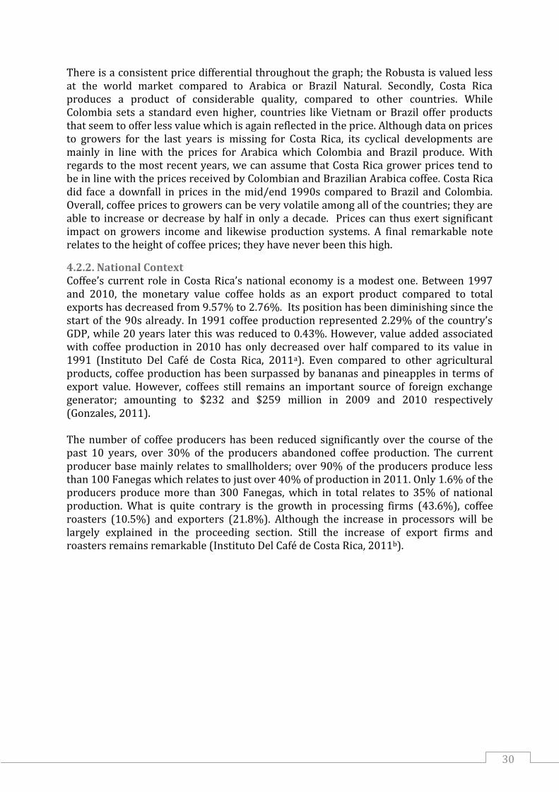
4.3 Research Region ............................................................................................................................... 33

7

4.4 Value Chain ......................................................................................................................................... 35

4.4.1 The Coffee Value Chain ........................................................................................................... 35

4.4.2 The Cooperative ........................................................................................................................ 36

4.4.3 Diversified Buyers & Processors ........................................................................................ 38

5. Discussion & Data Analysis ................................................................................................................... 40

5.1 Economics of Coffee Production ................................................................................................. 40

5.1.1. Farm Resources ........................................................................................................................ 42

5.1.2. Differentiating between Farm Resources .......... Error! Bookmark not defined.

5.1.3. Expenditures on Input ........................................................................................................... 46

5.1.4. Labour Costs .............................................................................................................................. 46

5.2. Off-Farm Income .............................................................................................................................. 54

5.3. Credit .................................................................................................................................................... 54

5.4 Incorporating an Environmental Dimension in Production ............................................ 47

5.4.1. Exploring the Degree of Sustainability............................................................................ 47

5.4.2. Characteristics of Sustainable Producers ...................................................................... 49

5.4.3 Sustainability and Value Chain Analysis .......................................................................... 50

5.4.4. Coffee Producers and Environmental Services ............................................................ 53

6. Limitations. ................................................................................................................................................. 54

6.1 Addressing Multi-Collinearity; Factor Analysis .................................................................... 68

6.2 Addressing Multi-Collinearity; Factors & Regression Analysis ...................................... 69

6.3 The Level on Sustainability .......................................................................................................... 70

7. Conclusion ................................................................................................................................................... 57

8. References ................................................................................................................................................... 59

9. Appendices .................................................................................................................................................. 65

Appendix 1. Elaborate Discussion on TCE and GVC Theory ................................................... 65

Appendix 2. Map of Region Los Santos. ........................................................................................... 67

Appendix 3. Household Questionnaire ............................................................................................ 68

Appendix 4. SPSS Output Files ............................................................................................................ 68

Appendix 4.1. Multiple Regression Analysis Differentiated Farm Resources ............. 74

Appendix 4.2. Multiple Regression Analysis Expenditures on Farm Inputs. ............... 75

Appendix 4.3. Multiple Regression Analysis Labour Costs ................................................. 76

Appendix 4.4. Partial Correlation; Loan Size controlling Land Size/Harvest. ............. 77

Appendix 4.5. Regression Model Contribution of Sustainability to Harvest. ...... Error! Bookmark not defined.

Appendix 4.6. Multiple Regression on Degree of Sustainability ....................................... 78

Appendix 4.7. Kolmogorov-Smirnov Test on Related Variables ....................................... 79

Appendix 4.8. Kendall’s Tau Correlation for Producer Rank on Sustainability .......... 80

8

Appendix 4.8. Kendall’s Tau Correlation for Producer Rank on Sustainability (Continued) ............................................................................................................................................ 81

9

1. Introduction

1.1 Introduction This section is meant introduce the reader by providing some introductory notes which intend to explain the research context and its motive. In this chapter we will elaborate on the 1) research context, 2) explaining the original focus of this study, 3) the main research questions, 4) justification for this research and 5) the outline of this thesis. We will proceed by discussing the research context.

1.2 Research Context Market integration is determined by several endogenous and exogenous conditions with respect to the production itself, which yields different levels of success within a specific sector. The Global Commodity Chain (GCC) approach (Gereffi, 1994) has been developed to analyse and understand the dynamics related to globalization, the market strategies implemented by different actors, and the effects of such strategies in developing countries, in special. The Global Value Chain (GVC) (Gereffi, Humphrey & Sturgeon, 2005) goes beyond production itself and gives a broader analytical context, where power structures, governance and actors strategies become relevant. In this sense, the approaches all consider the four classical dimensions defined by Gereffi: (1) The input/output system, (2) the geographical dimension, (3) the institutional dimension and (4) the power distribution dimension. This approach has often been used, for developing country firms, to investigate another popular term in GVC literature: upgrading, which refers to making better products, improve efficiency or moving into more skilled activities (Humphrey & Schmitz, 2002a). By following this approach, CINPE has had experience in the analysis of several sector chains in Costa Rica and Central America, such as coffee, water melon, snow peas, coco nut, chayote, mango, and pepper. On his visit to CINPE in 2009, Gereffi suggested to broaden the GVC approach by including the following dimensions: (1) regional studies of chains, (2) labour, (3) the environment, and (4) livelihood strategies. In this sense, the project “Environmental Services and Rural Space Use” (SERENA), a joint-research effort between CIRAD and CINPE, is interested to explore the environmental dimension of agricultural value chains and its effects on rural communities’ livelihoods. SERENA is a multidisciplinary project (int. al. economics, agronomy, sociology, policy making, geography) which investigates the concept of Payment for Environmental Services (PES) more closely. The theory on environmental services (sometimes referred to as ‘Ecosystem Services’) can be defined as the benefits, both direct and indirect, which people obtain from the environment. These services are the conditions and processes through which the entire environment sustain and fulfil human life. These services can be divided into several categories; provisioning, regulating, cultural and supporting (Millennium Ecosystem Assessment, 2005). The objective of the project SERENA is to identify the principles, mechanisms and instruments which facilitate the effective integration of PES and public policy (CIRAD, 2011). A key research subject in SERENA is the implementation and performance of market-based instruments aimed to incorporate the environmental dimension into the production and marketing of agricultural commodities. As a consequence, the use of grades and standards has become an important issue. In specific, the production and marketing of organic/sustainable agriculture is of great interest for the SERENA project. This thesis will focus on this subsection of the project and should thus contribute to its

10

broader objective. The following part will intent to explain the focus of this study and how this progressed towards the research questions.

1.2.1. Focus of this Study The original focus of this study differed considerably before we have had any explorative interviews with experts (a.o Prado, 2011). Initially, we had meant to compare organic versus conventional production while focussing on certified vs. non-certified producers. The production of organic coffee used to be very common, at least before the financial crisis started in 2008. Due to decreasing profitability, a large number of certified organic producers ceased organic production and returned to conventional. Nowadays, the proportion of conventional, sustainable and organic have been estimated to be very limited; up to 60%, 38% and 2% respectively although exact numbers are missing (Jimenez, 2011). Many of the producers have seemed to move to a so called middle class of production namely ‘sustainable’. However, there does not seem to be a consensus on the definition of sustainable. Some consider it to be a specific type of certification (given out by the Ministry of Agriculture) and relate it to the requirements of the Preferred Supplier Program (PSP) which Starbucks set it up in Costa Rica (Saxton, No Year). Others consider sustainable to be a typology comprising of Bird Friendly certification, Fair Trade labelling and organic production (Ubieta, 2006). This is very noteworthy; due to the lack of certified organic producers and the absence of a clear definition on sustainability one thus needs to come up with a new method in order to compare producers concerning their degree of sustainability. As a consequence this remains an essential part of our study.

1.3 Research Questions Due to the complexity described above, it is essential to clarify what drives this movement of ‘sustainability’ or at least environmental friendly production that seems to be common under a considerable share of the producers. The aim of this research, and likewise the research questions, should therefore try to encounter and define different groups of producers within the sample while emphasising the environmental dimension in agriculture. More specifically, the specific objective of this research is to investigate what environmental services different agricultural producers try to obtain from the environment and how this is reflected into production economics.. Taken into consideration the above paragraph, several research questions are defined:

1. How is ‘sustainability’ reflected back into the production process and what are the main characteristics of sustainable producers?

2. What is the relation between different value chains and their corresponding degree of sustainability?

3. How do different coffee producers distinct themselves with regards to the different environmental services they intend to pursue?

The first research questions should differentiate between at least two different groups of producers by considering the practices they apply to their farm and likewise the level of sustainability among producers. We intend to describe these different producers in detail. We then take this one step further with the second question by investigating if the differences between producers are also reflected back in their choices in which value

11

chain to participate. This questions should clarify a possible relationship with different value chains and sustainability. With regards to the final research question; we aim to examine the reasons and benefits that agricultural producers want to acquire with sustainable production. This question relates to attitudes and motivations.

1.4 Justification Beside the contribution which this thesis should yield to the overall objective of the project (SERENA), there other justifications for this study as well. This thesis investigates sustainable agriculture among coffee producers. The inclusion of this environmental dimension into agricultural value chains could provide insight and likewise new methods to combine environmental conservation while pursuing sufficient income for agricultural producers. In addition, the method brought forward into this thesis with regards to defining sustainable producers could be a tool to differentiate between producers more easily.

1.5 Outline of this Thesis The next chapter will provide a theoretical background on value chains and especially sustainable agriculture. The proceeding chapter will discuss our method by elaborating on the research activities and we have designed the research phase. This chapter will also address our approach with regards to differentiating between producers concerning their degree of sustainability. Afterwards we will discuss the Costa Rican coffee sector which includes a short market overview, an overview on our research region and a description of the different coffee value chains. Afterwards we will proceed by analysing and discussing our research sample; general agricultural economics on coffee production is explored first and afterwards we incorporate a focus on the environmental dimension. Especially this later focus should enable us to answer the research questions we have set earlier. After the analysis we have added a section that is meant to indicate the limitations to our research. After pointing out the main limitations we also try to resolve these in the same section. Afterwards we finish by providing the conclusions.

12

2. Theoretical Background

2.1. Introduction The theoretical context that one needs to consider relates mostly to a chain concept. Although there is a wide array of concepts which entail a point of view directed towards a chain (a.o. supply chain, production chain, Agro-food chain, value chain etc.) We will focus on the Global Value Chain (GVC) concept, due to its emphasis on developmental issues, in section 2. The GVC model lends itself well for examining an environmental dimension; we will extend this model in section 3 of this chapter. This section will first discus the roll of the environment in GVC analysis and how the environment should be incorporated in research on value chains. Afterwards we will discuss a popular method for incorporating environmental concerns into the ‘actual’ value chains; namely standards and certifications. We will proceed by summarizing similar research that investigated the characteristics and effects of sustainable agriculture. We will conclude by discussing a theory that should provide insight into motivations and benefits that producers can receive in case of sustainable production and in agriculture itself.

2.2. GCC and GVC Approach Due to its ability to include an environmental dimension, our main focus is on the GVC model. However, this model mainly originated from the Global Commodity Chain (GCC) model. Discussing the GVC model requires an explanation of the GCC model first.

2.2.1 The GCC Model The concept was first developed by Hopkins and Wallerstein and then it focussed primarily on the power of countries to influence global production systems by means of tariffs and local content rules. Gereffi and Korzeniewicz (1994, quoted by Sturgeon, 2008) revived the concept by focussing on firm strategies and their influence on shaping production systems. Global commodity chains are referred to as ‘sets of inter-organisational networks clustered around one commodity or product, linking households, enterprises and states to one another within the world economy’ as described by Gereffi & Korzeniewicz (Pelupessy & van Kempen, 2005). A GCC framework focuses on four main dimensions of analysis; input-output analysis, geographical area, institutional framework and chain governance (Gibbon, 2001). The first two have mainly been used descriptively in order to outline how chains are configured. The latest has attracted most of the attention among researchers and especially with regards to which actors are holding most of the power (driveness). Kaplinsky & Morris (2003) provide a concise governance characterization which is useful to consider first; Legislative This aspect relates to standard-setting and defining conditions for participation in

the chain. They may reside as legal rules, international rules or e.g. HACCP for food processing chains especially.

Judicial This part describes the governance related to audit performance and monitor

whether rules are complying to. Executive This part refers to the pro-active part of governance (i.e. actually executing

governance activities) in order to assist supplier to meet standards through direct

13

(helping supplier directly through e.g. manuals/training) or indirect assistance (forcing a first-tier supplier to help a second-tier supplier.

Gereffi (2001a) refers to specific forms of chain governance by providing two distinct types of governance structures; namely producer-driven and buyer-driven commodity chains. The first refers to a chain structure in which a large manufacturer influences production networks. This is mainly the case for capital or technology intensive industries such as the automobile sector. The source of large manufacturers’ lies in the control they hold over the backward and forwards linkages due to the high entry barriers in such technology intensive chains. Buyer driven chains on the other hand are dominated by large powerful retailers as well as successful branded merchandisers. The volume of their orders gives them significant power over other actors in terms of what, how, when and by whom the goods they sell are produced. As well as their position as an intermediary between overseas factories and niche markets in developed countries. They separated physical production and marketing/design and have likewise become manufacturers without factories; most of the value is added during the marketing and design stage (Gereffi, 2002). Although there is no direct link with the theory on the GCC model and our research, the following GVC model does and it has originated from the GCC model. Furthermore, it is worthwhile to discuss this part in detail because governance in chains can exert a considerable impact on primary producers. The following section will explain the GVC model and how it increased pressure on (developing) country producers.

2.2.2 The GVC Model The GVC model departs from the GCC model when it became increasingly difficult to indicate its governance structure; to label a chain either producer or buyer driven (Ponte & Gibbon, 2005). This is mostly due to recent developments with regards to 1) improved technology on the codification of information, 2) flexible capital equipment which is decreasing asset specificity, 3) labour intensive industries becoming more technologically enhanced and 4) increasing convergence of retailers’ and producers’ activities (e.g. private labels) (Sturgeon, 2008). Especially the first point is a major driving force and has often been led back to the internet (Gereffi, 2001b). What it basically runs down to is the increased disclosure and availability of information and standards. A very noteworthy statement is made by Gereffi (2001b, p.1628) when he specifically refers to ‘information asymmetry’. This enables us to differentiate between the GCC and GVC model by considering the theory on Transaction Costs Economics (TCE). For a more elaborate analysis of TCE and how it clarifies the link between GCC and GVC analysis we refer to appendix 1. The recent developments, leading to the GVC model, can be partially be interpreted as decreasing transaction costs. As a consequence, activities have become more dispersed in the chain and there is a stronger focus on firm linkages in the GVC model instead of an overall chain governance structure focussing on ‘driveness’ in the GCC model (Pietrobelli & Saliola, 2007). One can thus also expect that this is to be reflected in the governance structures. Gereffi, Humphrey and Sturgeon (2005) provided a clear table which elaborates on the different types of governance specific for the GVC model.

14

Figure 1. GVC Governance Types (Gereffi, Humphrey & Sturgeon, 2005) Considering the driving forces which are stated horizontally on the table, the main characteristics of these governance types are the following: Market - Governance type regulated by market linkages; repeat transactions and low switching costs. Modular Value Chains - Supplier produce according to more or less detailed specifications; do not require significant capabilities to translate. Relational Value Chains - High degree of asset specificity, complexity of relationships and mutual dependency. Often involve family or ethnic ties, geographical proximity or trust/reputation. Captive Value Chains - High dependency of small suppliers, due to high switching costs, on lead firms which impose strict monitoring and control. Hierarchy - High level of managerial control initiated by headquarters towards subsidiaries and other affiliates (fits well to vertical integration). To summarize, if one agrees that the driving forces (depicted horizontally on the table) address the prevalence of transaction costs, decreasing transaction costs leaves more room for joint value creation. As a consequence, the governance structures in the GVC model can be interpreted to be a trade-off between bearing risks/incurring costs (i.e. transactions costs) and the amount of joint value creation (i.e. transactional value).

2.3. Incorporating an Environmental Dimension

2.3.1. Introduction In a value chain where firms rely more on supplier capabilities, new and more stringent requirements are enforced on suppliers. Especially producers in developing countries face difficulties meeting these new requirements on e.g. product quality and characteristics, environmental conservation and labour standards which often do not apply to their domestic markets (Humphrey & Schmitz, 2008). Complying to these new requirements can also referred to as ‘upgrading’; which refers to making better products, produce existing products more efficiently or move into new activities (Humphrey & Schmitz, 2002a). Complying to standards on environmental conservation is just one possible strategy if one is looking to upgrade. There is a more precise characterisation that elaborates on the type of upgrading activities (Humphrey & Schmitz, 2002b):

15

Process Upgrading: Reorganizing the production system or introducing a new production technology to pursue e.g. more efficient input-output transformation. Product Upgrading: Firms can focus on producing product which generates more value added per employee which can be achieved by e.g. repositioning the entire chain to higher value products (niche markets). Functional Upgrading: This point relates to focussing more on new functions which are located in other parts of the chain e.g. marketing/design. The GVC model is able to examine how different governance types can result in opportunities for developing country firms and farms to upgrade (Ponte, 2008). Lead firms can play a very dominant role in GVCs and can likewise impede or allow developing country producer to learn, innovate and/or upgrade (Schmitz & Knorringa, 2000). However, this race between developing country firms trying to compete with each other to gain access into the chain or upgrade their activities can exerts an exhaustive influence on certain production factors and likewise the environment (e.g. land).

2.3.2 The Environmental Dimension in GVC Analysis Few studies consider the impact of GVCs on poverty, gender or the environment according to Bolwig et al. (2010). These issues are referred to as ‘Horizontal Elements’ in the chain; they concern elements that relate to only one specific actor or stage across different value chains. In this case all primary producers for different crops; poverty, gender and the environment extend themselves horizontally to all primary producers. Contrary to vertical elements in the chain, they refer to the phases necessary to transfer and process products starting from primary production and ending at consumer in only one specific chain. Bolwig et al. (2010) offers a conceptual framework which tries to incorporate a.o. an environmental dimension in GVC analysis. Value chains interact with the environment in 1) the primary production stage which utilizes the local resource base (soil, water, biodiversity) as well as in 2) the subsequent stage where nutrients, toxic substances and greenhouse gasses are released during production, processing, transport and other relevant activities inherent to a specific value chain. One can also look at this twofold by considering a geographical division namely 1) local processes and 2) global processes (although this approach is fairly similar to the twofold mentioned in the previous sentence). The first concerns mainly local natural resource management, water availability, contamination, positive or negative impacts on biodiversity and the later concerns processes which extent the value chain or national borders such as emissions of GHGs or toxic substances. Relevant topics to focus on could include e.g. the effect of excluding certain actors (exporters/processors) on land use or soil fertility. But how can we apply this framework to our case? This can be achieved by considering ‘upgrading’ in a broader sense. When a producer for example intents to access a certified organic export market it would require an improvement in product quality and a process upgrading (traceability). In a sense, complying to standards/certification on environmental issues can also be considered (process) upgrading (Fold & Larsen, 2011). In addition, rewards and risk stemming from upgrading can be understood both in financial terms but also in relation to poverty, gender and in particular the environment. In our case, we need to focus on revealing the effects which each production system has under different conditions i.e. before and after switching from conventional to

16

sustainable production (Rijsgaard et al, 2010). Switching from conventional to sustainable production is often achieved by introducing certification standards; and the effects of switching to certified production has been researched extensively. The following section will examine articles that investigated these effects.

2.3.3. Sustainable Practices, Standards & Certification A common strategy for including an environmental dimension in agricultural value chains has been achieved through the introduction of social, labour and environmental standards and certification. These standards include specifications related to environmental impact, improved working conditions and smallholder rewards (Bolwig, 2010). Standards can provide producers access to foreign market segments, enhance product value, acquire new functions and initiate closer cooperation with other actors in the chain. However, it can also create new entry barriers and present new challenges for existing suppliers (Jaffee, 2003). One of the most relevant standards in the coffee sector are the ones set by Starbucks’ PSP. All primary producers are required to comply to specific product quality, environmental and economic accountability standards (Starbucks Coffee Company, 2007). In addition, primary producers can acquire this certification based on a flexible point system. For primary producers a total of 80 points are divided equally among two categories; ‘Social Responsibility’ and ‘Environmental Leadership’. Producers have to achieve a minimum of 60% of the points for both the categories ‘Social Responsibility’ and ‘Environmental Leadership’ in order to qualify for preferred suppliers and 80% for becoming a strategic supplier. The table below summarizes the scorecard for primary producers for the category ‘Environmental Leadership’ only. Table 1. Division of Starbucks Points Category Division of

Points Objectives Division of Points

Protecting Water Resources

12 30% Water Course Protection 5 12.5% Water Quality Protection 4 10% Water Resources 3 7.5%

Protecting Soil Resources

12 30% Controlling Surface Erosion 7 17.5% Maintaining Soil Productivity

5 12.5%

Conserving Biodiversity

8 20% Maintaining Shade 4 10% Protecting Wildlife 2 5% Conservation Areas 2 5%

Environmental Management & Monitoring

8 20% Ecological Pest & Disease Control

5 12.5%

Farm Management 3 7.5% Complying to the most prevalent sustainable practices rewards the most points. Starbucks emphasis the conservation of soil and water resources while complying with the categories labelled ‘Conserving Biodiversity’ and ‘Farm Management & Monitoring’ is less rewarding. The latter mainly refers to the overall management structure of the farm; the allocation of resources, financial bookkeeping etc. What is noteworthy is that Starbucks provides objectives for the entire value chain, they do not elaborate on the practices or strategies which enables one to reach that objective. Clear practices are lacking, nor is there a justification why a specific category is rewarded more points

17

compared to others. Ramirez (2009) elaborates on sustainable coffee cultivation and provides a clear overview of sustainable practices. The table to the right displays these specific practices. Table 2. Sustainable Practices (Ramirez, 2009)

Agronomical Conservation Physical Conservation

Contour Planting Diversion Canals Live Barriers Exiting Canals Live Coverage Hillside Drainage Mulching Bench Terraces Shadow Provision / Trees Individual Terraces Application of Drawers in Canals These practices intend to conserve the soil and prevent erosion caused by water. In addition, the book discusses technical matters related to coffee cultivation; general practices like pruning, planting coffee, treatment with different varieties of coffee on different types of soil etc. A significant part of the book by Ramirez (2009) is devoted to the use of shade/planting trees in the coffee plot. The standards used by certifier Rainforest Alliance (RA) provide a far more elaborate and stringent framework but it is not strictly confined to coffee cultivation. Certification from RA is a socio-environmental standard focussing on production practices incorporating social requirements as well. Farmers do not have to be certified organic or practice organic methods, it is thus not as strict as organic but producers cannot use any chemical or non-organic input (Subieta, 2006). In addition, they are required to follow an integrated pest management strategy, are not allowed to use pesticides banned in the US or EU and must continue to reduce their pesticide use. Regulations regarding wildlife conservation are strict and producers must also adhere to strict requirements with regards to the provision of shade (Sustainable Agricultural Standards, 2010). Contrary to Starbucks, RA does not allow producers to be certified in collectives (e.g. cooperatives); making it more expensive. This is mainly why producers are reluctant to adhere to RA requirements.

2.3.4. Organic & Sustainable Agriculture Before examining the effects of sustainable or certified agricultural production, we first need to define sustainability. It seems hard to reach a consensus over the definition of ‘sustainability’ or ‘sustainable agriculture’. In a quickly changing world, anything can become sustainable. In agriculture, sustainability can be defined as (Duesterhaus, 1990): “farming systems that are capable of maintaining their productivity and usefulness to society. Such systems must be resource conserving, socially supportive, commercially competitive and environmentally sound” However, the term sustainability has been applied to assess organic agriculture as well. But then again, this is not in conflict with the definition given on the previous page. It does create some confusion when discussing sustainability as a whole. One example includes Van der Vossen (2005); he analysis the sustainability of organic coffee production while considering agronomic (a.o. plant nutrients, soil organic matter, soil quality etc.) and economical aspects (e.g. profit, yield, input costs etc.). He concluded that organic production in its present form does not sustain coffee production. Nutrient

18

cycling processes seem to remain fairly similar under conventional and organic production; additional inputs of inorganic (i.e. synthetic) fertilizer seem to be necessary in order to achieve sufficient yields and balanced plant nutrient flows. In addition, negative nutrient balances (depleting soil nutrients) in shaded coffee farms is likely if one limits itself to organic fertilizers only. Moreover, organic fertilizers are not sufficiently available and rich in terms of nutrient content, one thus needs to acquire considerable amounts of organic fertilizer. Smallholders lack the resources necessary to acquire enough organic fertilizers on a regular basis. This is reflected in the yield; the price premium is unable to compensate the additional costs and decreasing yield with organic production. Net income on organic farms is about 25-50% lower as compared to conventional farms. These arguments are in line with the statements made by Valkila (2009) arguing that low intensity organic farming, and the associated lower yield, might even become a poverty trap for small marginal producers. And this statement seems to be more relevant in case of low world market prices. A question that comes up as well is ‘What do we want to sustain?’. There have been more specific accounts on what sustainability has to adhere to or at least what it needs to sustain (Gold, 2007):

1. Satisfy human food and fibre needs. 2. Enhance environmental quality and the natural resource base upon which

the agricultural economy depends. 3. Efficiently utilise non-renewable resources and on-farm resources and

incorporate biological cycles and control. 4. Maintain economic viability of the farm. 5. Improve the quality of life for farmers and society as a whole.

Clearly there is a mixture of environmental, social and economic objectives. However, interpretation of e.g. ‘efficiently’, ‘quality of life’ and ‘environmental quality’ can differ considerably in different contexts. The available literature often applies a focus that can be very diverse as well. It seems as that a primary force for the introduction of sustainable agricultural methods in a production systems, or at least raising a level of awareness, is the contact with third-parties such as NGOs, donors, producer cooperations etc. They mainly encourage sustainable production, followed by raising producer capacities, creating market access and stabilizing producer environment (i.e. fair trade)(Bitzer et al., 2008). The dimensions on what to sustain has also offered different dimensions of analysis. Research on the social (working conditions for agricultural labourers, workers knowledge and access to health care) and environmental dimensions (conservation of biodiversity, management of water resources, waste management and pesticide handling) which has been conducted by De Lima et al. (2009) does not include the economic dimension. They have come up with results that favour the introduction of standards implied by Rainforest Alliance when comparing certified farmers with a control group of non-certified farmers. The requirements improved working conditions, length of employment and pesticide handling but it failed to deliver a positive impact on the provision of health care to labourers. With regards to the environment; waste management, water resource management and conserving biodiversity are also positively associated with certification by Rainforest Alliance. However, one can also

19

zoom in and investigate the results on economic aspects only (as opposed to results in environmental or social aspect) stemming from one specific sustainable practice. Gobbi (1999) researched financial viability of five different production systems ranging from ‘Intensive Monoculture & no Shade Trees – Few Coffee Plants & Many Shade Trees’. The monoculture system makes no use of shade trees and coffee plants are fully exposed to the sun while with each proceeding method the number of coffee plants per hectare decrease while the amount shade trees per hectare increase. All of the production systems seem to be financially viable, although investments differ. It is most expensive progressing from a monoculture to a method in which many shade trees per hectare are incorporated. However, the amount of shade trees does not seem to affect yield significantly. A considerable amount of literature consider ‘organic’ production and then analyses the sustainability of such production systems. The requirements related to organic production are more stringent and specific than characteristics related to sustainability. Sustainability does not necessarily oblige farmer to adhere to specific requirements; it is often a term used to assess a specific situation concerning its ability to preserve specific aspects (environmental quality, income levels etc.) and likewise can also be applied to asses organic production. Requirements related to organic agriculture are mostly set by the International Federation of Organic Agricultural Movement (2006) and include the following:

1. Use of composted organic matter to improve soil quality; no synthetic fertilizers. 2. Introduction of soil conservation techniques, for example contour planting,

terracing, cover crops, mulch and shade trees. 3. Natural disease, pest and weed control; no synthetic pesticides. 4. Minimal use of fossil fuels during production. 5. Minimal environmental pollution during post-harvest handling.

Analysis on organic agriculture shows contrasting results. Calo and Wise (2005) reveal that in case of low coffee prices all producers are facing a hard time. It is making it especially hard for producer in transition; where they are meant to produce ‘organically’ already but are not certified as such and likewise do not receive the premium. They are facing costs which are almost 3 times higher per kg. of coffee compared to the price they receive per kg. of coffee. Although certified organic farmers experience more negative returns per hectare than conventional farmers, they still are able to cover more costs since they experience less net losses. In another case, investments in organic production is worthwhile. Although per tree production is lower under organic production as compared to conventional production and variable costs are slightly higher for organic production, the price premium does seem to cover the income loss compared to changing from conventional production (Lyngbaek et al., 2001). However, in other cases this is the opposite. In Costa Rica, coffee production is already highly dependent on chemicals and transforming to organic production bears a significant initial investment as well as production losses. Mainly younger and well educated farmers decide to produce organically and to apply for certification. Moreover organic producers mainly include larger farmers; smallholders are less likely to apply for organic certification (Blackman & Naranjo, 2010). In addition, those that mainly devote to sustainable production seem to be more entrepreneurial as well. They are more likely to adopt new farming practices and earn more off-farm income, contrary to conventional producers

20

who acquire more income solely derived from the production of coffee (Comer et al., 1999).

The analysis by Kilian et al. might yield insights into why the analysis on the economical situation under organic/sustainable in the articles mentioned earlier tend to differ. In Latin America, although most countries face similar yield, costs on input and labour are considerably higher in Costa Rica for organic production ($2.700 per hectare). While organic producers in Guatemala are facing only $2.000 per hectare and Honduras and El Salvador even less than 1.500 per hectare. All of them require different prices per pound of coffee in order to break even. In addition, it also depends on what certification standards one is considering. Fair-trade, Rainforest Alliance, UTZ Certified and Organic certification all incorporate some degree of social, environmental and economic standards (although some implies more strict/rigid standards than others). All these certifications method can be interpreted as sustainable but they differ in terms of the price premium they provide farmers. On average, organic producers receive $0,15-0,25 price premium per pound of coffee. Rainforest Alliance incorporates a premium of $0,15 per pound of coffee to producers while Fair-trade producers receive $0,62 price premium per pound. UTZ Certified only $0,07 per pound of coffee. As a consequence, analysis might differ significantly depending on the country of analysis and the certification method.

Finally, participation in such speciality markets such as organic or fair trade can yield considerable benefits. It is a useful tool to cope with crises. Participation in speciality markets has a greater influence on the price which farmer receive than coffee bean quality (mostly associated with altitude). Cooperatives can play an important role; they tend to enable farmers to receive better prices. As a consequence, producers submitting their coffee to cooperatives who sell to specialty markets perceive the risks of losing the title on their land due to low coffee prices 4 times smaller as compared to producers selling their coffee to conventional markets (Bacon, 2005).

2.3.5. Environmental Services But to what extent will it be able to explain why producers opted for sustainable agriculture? The theory on environmental services (sometimes referred to as ‘Ecosystem Services’) is able clarify this issue. Environmental services can be defined as the benefits, both direct and indirect, which people obtain from the environment. These services are the conditions and processes through which the entire environment sustain and fulfils human life (Millennium Ecosystem Assessment, 2005). They are divided into several categories; provisioning, regulating, supporting and cultural (table #).

21

Figure 2. Environmental Services (Millennium Ecosystem Assessment, 2005) Provisioning services refer to the products obtained from the environment while regulating services relate to the benefits obtained from the regulation of environmental process. Cultural services include nonmaterial benefits such as recreation, spiritual enrichment, reflection etc. Supporting services refer to services necessary for the functioning of the previous three dimensions (e.g. production of oxygen, nutrient cycling, primary production etc.). These environmental services do offer a ground for comparing them with sustainable practices and certification standards. These services refer to conditions and processes through which the environment sustains human life. Agricultural production serves the same goal; needless to say that agricultural production requires numerous environmental services and at the same time are a channel through which humans receive environmental services. When someone considers only conventional production, (focussing only on the production of crops) the most relevant environmental services pertains to ‘Provisioning Services’ namely ‘Food’, ‘Fibre’ and ‘Fuel’ etc. However, addressing sustainable production methods includes more environmental services than just provisioning services. If one relates the practices by Ramirez (2009) mentioned in the previous section with the environmental services, there are more links. The conservation of soil by means of ‘Live Soil Coverage’, ‘Live Barriers’ and ‘Trees’ mainly relate to the ‘Erosion Control’ pertaining to ‘Regulating ‘Services’. While ‘Terracing’, ‘Construction of Canals’, ‘Drainage’ and ‘Drawers in Canals’ focus more on ‘Water Regulation’. In addition, applying ‘Organic Fertilizer’ can contribute to ‘Nutrient Cycling’ which relates mostly to ‘Supporting Services’. In conclusion, comparing sustainable coffee practices to conventional production, the first seems to address and require a wider array of environmental services. Environmental services could also be of help to reveal how sustainable production is being motivated from the primary producers’ point of view. This could be achieved by Enquiring why producers produce sustainably by asking what benefits they pursue and later compare this to the practices they apply.

22

3. Methodology

3.1 Introduction This chapter is meant to summarize the research phase and how it was conducted. The following chapter aims to clarify how and why we conducted this research by elaborating on our primary and secondary sources. In addition, the proceeding section will discuss the approach with which we intended to differentiate between coffee producers concerning their degree of sustainability.

3.1.1 Literature Study An exploratory study on the theory was conducted in order to introduce the topic. The analysis of secondary data can enhance primary data; one must familiarize itself with the topic at hand and secondary data enables one to identify concepts, data and terminology that can be useful while conducting primary research as well (Burns & Bush, 2006). The data which has been considered in this research mainly include reports, journals, books and statistics. The latter mainly includes statistics of Costa Rica on the coffee sector, the different coffee producing regions, the prevalence of sustainable/organic producers. The main concepts which have been studied include sustainable agriculture, environmental services, standards, certification and (sustainable) agricultural practices. This literature study was conducted before and after the research period. Reviewing theory after the research is carried out, is meant to find support for our findings.

3.1.2 Structured Interviews Besides reviewing literature in order to prepare oneself, it is worthwhile to consult experts. We conducted several exploratory interviews to familiarize ourselves with the coffee sector, common practices, prevalence of organic production and the research region at hand. We also explained the objective of our research, enquired to the presence of similar research and other experts knowledgeable of our research topic. The interviews include the regional coordinator in Los Santos for the Instituto del Café de Costa Rica (Icafé) Adrian Gamboa, a research consultant Rodrigo Jimenez and an owner of a microprocessor Rafael Prado. All of these interviews have been recorded, typed out and analysed afterwards.

3.1.3 Pre test Before commencing the actual research period, we conducted several feedback and pre-test interviews. We conducted exploratory, feedback interviews with an agronomist from the cooperative Llano Bonito and the owner of a microprocessor. Their feedback on possible challenges, difficulties and problems which we could encounter in the field enabled us to create an efficient questionnaire. The questionnaire was then pre-tested on a member of the cooperative which forced us to rethink the outline of the survey as well as to reduce its overall size (with regards to overlapping, similar or redundant questions).

3.1.4 Sample & Study Site The selection of the study site was achieved after several meetings with different experts and researcher of CINPE. The area has been chosen due to the high number of coffee producers in a relatively small region. This is meant to significantly reduce

23

travelling time between respondents and to acquire a large sample in an efficient way. The majority of people living there, dedicate themselves to the production of coffee. The data collection method we have used can be referred to as the snowballing method. We were not able to obtain a list of producers mainly because the cooperative did not held records of their members. The snowballing method, which enables one to get to populations which are difficult to reach, is thus a worthwhile strategy. It enables one to acquire knowledge on respondents and helps locating them as well and to gather information on respondents that we would otherwise not have known by enquiring among respondents themselves. However, snowballing also has the potential to introduce several biases in the sample. Since one is not aware if the sample is an accurate representation of the target population it can severely limit representativeness. In addition, selecting respondents is out of control of the researcher. The initial subjects which have been researcher tend to suggest subject that share similar traits possibly leading to a sample that can be rather homogenous (Burns & Bush, 2006). As a consequence one cannot generalize statistically significant results that have come out of the sample to a larger population. Therefore, we have to limit our conclusions to our sample only. Nevertheless, providing analyses and conclusions is still worthwhile because this sample on itself can bring forward new and interesting results that can be compared to coffee producers in other regions that hold different traits e.g. geographical characteristics. Furthermore, it does assist the cooperative from which we have received help to acquire an overview and in-depth information on their members. We initiated first contact with producers with the help of a Cooperative (Coope LlanoBonito) and the owner of a microprocessor. Afterwards, we succeeded into addressing producers with the help of the ones we have previously interviewed. Since the contact of the micro processor were quite limited we mainly relied on respondents that were encountered via the cooperative. According to their own website1, the number of members of the cooperative amount to 630 coffee producers. While the cooperative mentions that they are certified Fair-trade and ‘Sustainable Coffee’, hardly any producer is aware of being certified and if so, what certification they have. We structured and planned the interviews by considering the location; mainly conducting interviews with 5-6 producers (living in the same village) per day. Employees of the cooperative helped us with targeting and mapping coffee producers by differentiating between communities in which they reside. We ended up interviewing a sample of 104 producers. This considerably influences the research and its outcome; its only a rather small share of a population mainly confined and related to the cooperative so we have to be cautious with regards to generalizing our results. In addition, the snowballing method can further increase the risk of the sample being homogenous .

3.1.5 Data Analysis Data was entered into survey printouts on the spot. Afterwards they have been codified and entered into SPSS 18.0 for further analysis.

1 http://www.llanobonito.com/nosotros.html

24

3.2 Addressing Sustainability among Producers

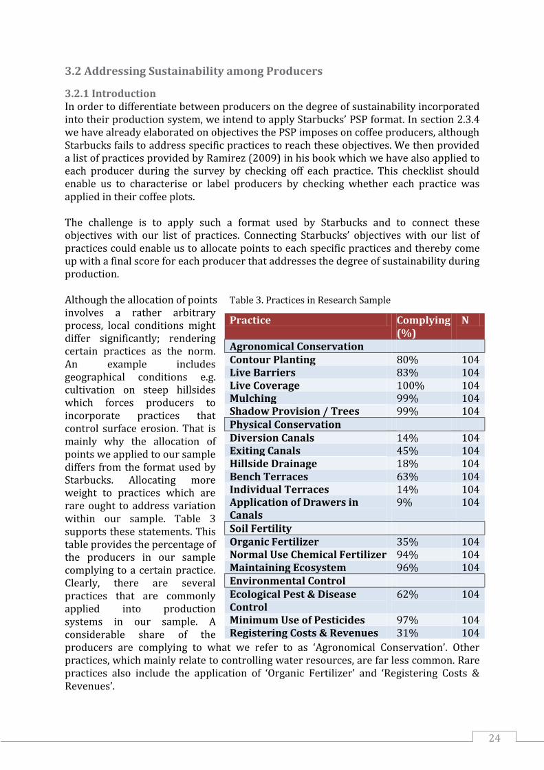
3.2.1 Introduction In order to differentiate between producers on the degree of sustainability incorporated into their production system, we intend to apply Starbucks’ PSP format. In section 2.3.4 we have already elaborated on objectives the PSP imposes on coffee producers, although Starbucks fails to address specific practices to reach these objectives. We then provided a list of practices provided by Ramirez (2009) in his book which we have also applied to each producer during the survey by checking off each practice. This checklist should enable us to characterise or label producers by checking whether each practice was applied in their coffee plots. The challenge is to apply such a format used by Starbucks and to connect these objectives with our list of practices. Connecting Starbucks’ objectives with our list of practices could enable us to allocate points to each specific practices and thereby come up with a final score for each producer that addresses the degree of sustainability during production. Although the allocation of points Table 3. Practices in Research Sample involves a rather arbitrary process, local conditions might differ significantly; rendering certain practices as the norm. An example includes geographical conditions e.g. cultivation on steep hillsides which forces producers to incorporate practices that control surface erosion. That is mainly why the allocation of points we applied to our sample differs from the format used by Starbucks. Allocating more weight to practices which are rare ought to address variation within our sample. Table 3 supports these statements. This table provides the percentage of the producers in our sample complying to a certain practice. Clearly, there are several practices that are commonly applied into production systems in our sample. A considerable share of the producers are complying to what we refer to as ‘Agronomical Conservation’. Other practices, which mainly relate to controlling water resources, are far less common. Rare practices also include the application of ‘Organic Fertilizer’ and ‘Registering Costs & Revenues’.

Practice Complying (%)

N

Agronomical Conservation Contour Planting 80% 104 Live Barriers 83% 104 Live Coverage 100% 104 Mulching 99% 104 Shadow Provision / Trees 99% 104 Physical Conservation Diversion Canals 14% 104 Exiting Canals 45% 104 Hillside Drainage 18% 104 Bench Terraces 63% 104 Individual Terraces 14% 104 Application of Drawers in Canals

9% 104

Soil Fertility Organic Fertilizer 35% 104 Normal Use Chemical Fertilizer 94% 104 Maintaining Ecosystem 96% 104 Environmental Control Ecological Pest & Disease Control

62% 104

Minimum Use of Pesticides 97% 104 Registering Costs & Revenues 31% 104

25

If one recalls the table discussing the allocation of points of Starbucks’ PSP in section 2.3.4, the categories ‘Protecting Soil Resources’ and ‘Protecting Water Resources’ carry equal weight. However, physical conservation practices which are assumed to relate mostly to ‘Protecting Water Resources’ are less prevalent in our sample than agronomical conservation practices which mostly relates to ‘Protecting Soil Resources’. These statements are in line with the characteristics of many of the plots; just over 5% of the plots were labelled as ‘Plane’. Almost 50% and 40% of the producers characterise the slope of their plot as mild or significant respectively. The perception on the risk of erosion in their plots tell fairly similar story. About 42% and 16% of the producer deem this risk to be moderate or high respectively. Over 40% consider this risk to be low. Table 4. Modified Point Division of Starbucks Standards

Category Division of Points

Objectives Division of Points

Protecting Water Resources

18 45% Water Course Protection 8 20% Water Quality Protection 8 20% Water Resources 2 5%

Protecting Soil Resources

13 32,5% Controlling Surface Erosion 7 17,5% Maintaining Soil Productivity

6 15%

Conserving Biodiversity

5 12,5% Maintaining Shade 2 5% Protecting Wildlife 2 5% Conservation Areas 1 2,5%

Environmental Management & Monitoring

4 10% Ecological Pest & Disease Control

1 2,5%

Farm Management 3 7,5& Because some practices are common and other rare, we have decided to modify the original allocation of points that was applied by Starbucks’ PSP. The table above depicts Starbucks’ PSP format but the division of points has been altered. The first category now carries most points. The category below (Protecting Soil Resources) carries less points than the first category but still more points compared to Starbucks’ PSP original division. The last two categories have been downsized significantly. The division of points for the column called ‘Objectives’ have been changed as well, depending on the practice they relate to. The next paragraph will further clarify this.

3.2.2 Configuring a Ranking-Approach The steps below clarify how we assigned points to each practice in our checklist.

1. Link Objectives with Practices The first step included linking each objective with practices that enable producers achieve those objectives. Complying to a specific practice sometimes resulted that producers were rewarded points from different objective. This also meant that when a producer has the objective to e.g. ‘Control Surface Erosion’ it needs to incorporate different practices.

2. Divide Points from the Objectives and Distributing them to Practices Because complying to a specific objective can be achieved by applying a set of practices, we examined the number of practices that enable a producer to achieve a specific

26

objective. If for example ‘Maintaining Soil Productivity’ can be achieved by applying 1) Mulching, 2) Live Coverage, 3) Organic Fertilizer and 4) Minimal Use of Chemical Fertilizer, the points (6) pertaining to this objective must be divided by 4. These 4 practices are rewarded 1.5 points each. However producers can be rewarded points from more than 1 objective if they apply a certain practice. Consider the example above; the practice ‘Organic Fertilizer’ is rewarded 1.5 points. However, applying organic fertilizer enables producers to achieve several objectives. The producer also achieves ‘Water Quality Protection’ because organic fertilizer contain less harmful nutrients that might deter water quality.

The objective ‘Water Quality Protection’ has gone through the second phase as well so for each practice that help producers achieve ‘Water Quality Protection’, we know the amount of points to be rewarded(i.e. 2 points). We can now calculate the amount of points organic fertiliser receives by adding up both the rewards that organic fertilizer receives from both these objectives, which is equal to 3.5 points.

3. Configuring final ‘Sustainability Score’ After allocating points to each practice, all these points need to be added up for each producer in order to come up with a final score that addresses the overall level of sustainability. Producers will be rewarded to total amount of points pertaining to a practice when complying to a specific practice while not applying yields no points. Point 2 and 3 can be confusing since it deals with both objectives and practices being applied more than once. Table 5 on the next page depicts the division of points, using the same format as section 3.2.1. for each practice and the relevant Starbucks’ objectives they address. The first column depicts the practices while the second one refers to the points rewarded when complying to each practice. The last column elaborates on the relevant objective(s) that relate to our practices. We have allowed the objectives ‘Controlling Surface Erosion’ and ‘Maintaining Soil Productivity’ pertaining to the category ‘Soil Resources’ to be linked with practices more often than ‘Water Resources’. That is mainly due to the prevalence of practices focussing on ‘Soil Resources’ which are already incorporated to a large extent among producers in our sample. The distribution of points above has already been incorporated into our SPSS database. This was done afterwards by translating the labels from ‘Yes’ or ‘No’ into a numerical value i.e. the specific amount of points to be obtained for a certain practice.

27

Table. 5. Practices, Division of Points and Starbucks Objectives

Practice Points Related Objectives Agronomical Conservation Contour Planting 1 Controlling Surface Erosion Live Barriers 1 Controlling Surface Erosion Live Coverage 1,5 Maintaining Soil Productivity Mulching 1,5 Maintaining Soil Productivity Shadow Provision / Trees 2 Maintaining Coffee Shade

Canopy Physical Conservation Diversion Canals 5 Controlling Surface Erosion

Water Quality Protection Water Course Protection

Exiting Canals 4 Water Quality Protection Water Course Protection

Hillside Drainage 3 Controlling Surface Erosion Water Resources & Irrigation

Bench Terraces 3 Controlling Surface Erosion Water Course Protection

Individual Terraces 3 Controlling Surface Erosion Water Course Protection

Drawer in Canals 3 Controlling Surface Erosion Water Quality Protection

Soil Fertility Organic Fertilizer 3,5 Maintaining Soil Productivity

Water Quality Protection Normal Chemical Fertilizer 1,5 Maintaining Soil Productivity Maintaining Ecosystem 1 Conservation Areas

Protecting Wildlife Environmental Control Ecological Pest & Disease Control

2 Protecting Wildlife Ecological Pest & Disease Control

Minimum Use Pesticides 1 Protecting Wildlife Registering Costs & Revenues

3 Farm Management & Monitoring

28

4. Coffee Sector

4.1 Historical Perspective The role of coffee as Costa Rica’s driving force behind developments dates back to the 19th century when coffee cultivation started to become more prevalent and export channels were created. Costa Rica, at that time only a province pertaining to a larger nation comprising of different central America countries, had to find a product which did not compete with other countries’ products neither with products in which Spain traded. If not, they would not obtain the permission from the government, seated in Guatemala, to trade in that specific crop. Coffee, at that time still a relatively new crop to Costa Rica, lend itself perfectly. The introduction was led back to the year 1809 when a priest received coffee beans brought from Jamaica from a befriended naval captain. He planted them the same year and a few years later, gave some coffee beans to poorer people as well while promoting and instructing them on coffee cultivation. In 1832 the first bag of coffee was exported to Chile and a year later coffee found its way to the United States, the United Kingdom, Peru and Nicaragua. From the mid-19th century, coffee became the only export product and the government decided to support coffee cultivation which included developing the necessary infrastructure (i.e. roads, railways etc.), stimulating production by providing access to credit (governmental banks) and acquiring more knowledge on e.g. production techniques. In 1855 production amounted to 70,000 Fanegas2 which was cultivated on 11,000 hectares, while by the end of the century production was fivefold; 350,000 Fanegas cultivated on 50,000 hectares. Halfway the 20th century, coffee production began to expand to regions outside the central valley region mainly towards the southeast and south of the capital (a.o. Guanacaste, Coto Brus). Coffee cultivation was mainly based on smallholder production while only a smaller share of the producers consisted of large scale producers, of which the latter faced higher yields per hectares compared to smallholders (Jimenez, 1998). More recent, but already in a sense historical, events have put a significant mark on the (global) coffee sector. Changing patterns in the global coffee commodity chain in the 1990s led to a coffee crisis and had far-reaching effects on producers in developing countries. Due to disintegration of the International Coffee Agreement in 1989, market liberalization, corporate consolidation and increasing production, prices plunged to their lowest level in a century. This had devastating effects on rural economies, biodiversity associated with traditional coffee production, employment rates and accelerated rural-urban migration (Bacon, 2006). Other claim that the plunge in world prices was mainly due to increasing supply of especially Robusta coffee from countries such as Vietnam or Brazil. Since coffee toasters are able to substitute Arabica and Robusta in their blends, price differentials between the two declined. Since Costa Rica mainly devoted itself to the production of Arabica, they also faced decreasing prices (Chaves & Solano, 2003). Producers had to cope with historically low prices throughout the 1990s. There have even been accounts that in Central America, in one year prices dropped with 44% (Eakin et al., 2006).

2 A Fanega is equal to 46 kilos unroasted coffee beans; outer ‘pulp’ or cherry is then already removed.

29

4.2 Current Market Situation The coffee market nowadays depicts a somewhat different story, especially in terms of its significance for the economy in Costa Rica. However, there are still regions which remain highly dependent on coffee production. When measuring production, common measuring units are ‘Fanegas’. A Fanega is a large wooden box which on average contains 258 kilo of coffee cherries which equals 46 kilos of green coffee beans (unroasted).

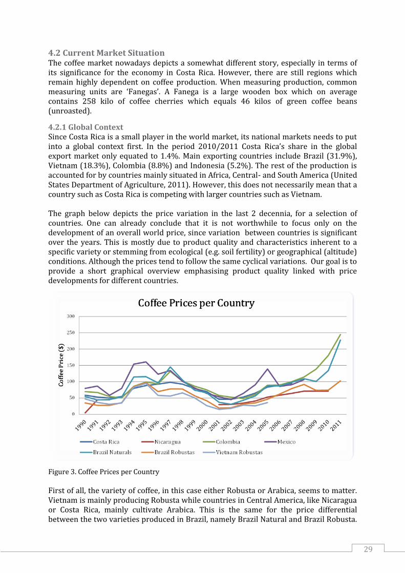
4.2.1 Global Context Since Costa Rica is a small player in the world market, its national markets needs to put into a global context first. In the period 2010/2011 Costa Rica’s share in the global export market only equated to 1.4%. Main exporting countries include Brazil (31.9%), Vietnam (18.3%), Colombia (8.8%) and Indonesia (5.2%). The rest of the production is accounted for by countries mainly situated in Africa, Central- and South America (United States Department of Agriculture, 2011). However, this does not necessarily mean that a country such as Costa Rica is competing with larger countries such as Vietnam. The graph below depicts the price variation in the last 2 decennia, for a selection of countries. One can already conclude that it is not worthwhile to focus only on the development of an overall world price, since variation between countries is significant over the years. This is mostly due to product quality and characteristics inherent to a specific variety or stemming from ecological (e.g. soil fertility) or geographical (altitude) conditions. Although the prices tend to follow the same cyclical variations. Our goal is to provide a short graphical overview emphasising product quality linked with price developments for different countries.

Figure 3. Coffee Prices per Country First of all, the variety of coffee, in this case either Robusta or Arabica, seems to matter. Vietnam is mainly producing Robusta while countries in Central America, like Nicaragua or Costa Rica, mainly cultivate Arabica. This is the same for the price differential between the two varieties produced in Brazil, namely Brazil Natural and Brazil Robusta.

30

There is a consistent price differential throughout the graph; the Robusta is valued less at the world market compared to Arabica or Brazil Natural. Secondly, Costa Rica produces a product of considerable quality, compared to other countries. While Colombia sets a standard even higher, countries like Vietnam or Brazil offer products that seem to offer less value which is again reflected in the price. Although data on prices to growers for the last years is missing for Costa Rica, its cyclical developments are mainly in line with the prices for Arabica which Colombia and Brazil produce. With regards to the most recent years, we can assume that Costa Rica grower prices tend to be in line with the prices received by Colombian and Brazilian Arabica coffee. Costa Rica did face a downfall in prices in the mid/end 1990s compared to Brazil and Colombia. Overall, coffee prices to growers can be very volatile among all of the countries; they are able to increase or decrease by half in only a decade. Prices can thus exert significant impact on growers income and likewise production systems. A final remarkable note relates to the height of coffee prices; they have never been this high.

4.2.2. National Context Coffee’s current role in Costa Rica’s national economy is a modest one. Between 1997 and 2010, the monetary value coffee holds as an export product compared to total exports has decreased from 9.57% to 2.76%. Its position has been diminishing since the start of the 90s already. In 1991 coffee production represented 2.29% of the country’s GDP, while 20 years later this was reduced to 0.43%. However, value added associated with coffee production in 2010 has only decreased over half compared to its value in 1991 (Instituto Del Café de Costa Rica, 2011a). Even compared to other agricultural products, coffee production has been surpassed by bananas and pineapples in terms of export value. However, coffees still remains an important source of foreign exchange generator; amounting to $232 and $259 million in 2009 and 2010 respectively (Gonzales, 2011). The number of coffee producers has been reduced significantly over the course of the past 10 years, over 30% of the producers abandoned coffee production. The current producer base mainly relates to smallholders; over 90% of the producers produce less than 100 Fanegas which relates to just over 40% of production in 2011. Only 1.6% of the producers produce more than 300 Fanegas, which in total relates to 35% of national production. What is quite contrary is the growth in processing firms (43.6%), coffee roasters (10.5%) and exporters (21.8%). Although the increase in processors will be largely explained in the proceeding section. Still the increase of export firms and roasters remains remarkable (Instituto Del Café de Costa Rica, 2011b).

31

0

1000

2000

3000

4000

5000

6000

7000

Fan

egas

(x1

00

0)

Production & Export

Export Production

The majority of national coffee production is meant for export purposes; approximately 85% while the rest is meant for national consumption. The graph below displays the production as well as the share which is exported. Production, and likewise export, face declining trends, setting in from the start of the millennia. Over half what is exported is shipped to the US (56.3%), while European countries account for 26.3%. Remarkable is the share taken by Belgium (11.2%), which seems to be able to acquire a considerable trading role. Other countries importing Costa Rican coffee include a.o. Japan (3.8%), Canada (2.9%) and Australia (2%). In the last 3 years, producers have witnessed a significant price increase for their coffee. Throughout the years 2009, 2010 and 2011 producers have witnessed a price increase of 8%, 12% and 39% respectively. It is only

Figure 4. Production & Export Volumes in Costa Rica

since recent that producers seem to have increased production. However, they have not been able to fully take advantage of this price increase due to detoriating value (on average 5% over the past two years) of their national currency against the dollar (Instituto Del Café de Costa Rica, 2011b).

4.3.3. Sustainable Market Overview The market for sustainable production has witnessed considerable growth the past few years. During 2004 – 2009 production increased with 433%. Sustainable coffee production in 2009 represented 17% of total coffee production. However, the share of sustainable coffee in export is considerably lower; only 8% of total export. Most of the certification types are equal in share; organic coffee (25.9%) is the largest followed by fair-trade (23.3%), Rainforest Alliance (22.3%), UTZ Certified (20.9%) and finally the 4C Association3 (7.5%). Considering regions only, Latin America is the main producer of sustainable coffee; 76.5% of all production resides in Latin American countries. While Asia account for a

3 A private partnership between CAFÉ Practices of Starbucks and the CCC program of Nespresso.

32

considerable lower share followed by Africa. Sustainable production per country is especially dominated by Brazil, Peru, Colombia and Vietnam (78%). Coffee prices tend to differ a lot among countries, these differentials are mainly based on internationally recognized quality and flavour associated with a specific country. The price premiums arising from certifications are measured as prices that earned above the ‘normal’ coffee prices per country. The price premiums per pound of green coffee among different certification method tend to differ as well. Fair-trade certification applies minimum pricing; in case of low world market prices4 producers do not experience significant volatility in income. In case of high world market price (above minimum prices) producers do not receive a Fair-trade margin, they face world market price and an additional social premium5. With regards to UTZ Certified, its price premium varies between $0.01 – $0.13 per pound of green coffee. Although on average producers receive $0.05 per pound of green coffee. For the 4C Association, producers acquire between $0.01 - $0.03 price premium per pound of green coffee. In the case of Rainforest Alliance and organic coffee; neither of them contain pricing requirements in their set of standards. Producers certified with Rainforest Alliance however receive $0.11 price premium per pound of green coffee. Producers face the highest price premium when producing organically; on average $0.29 per pound of green coffee (Potts et al., 2010).

4 $1.45 per pound for Arabica and $1.24 per pound for Robusta.

5 The social premium refer to an additional premium that must be reinvested in a project that benefits producers.

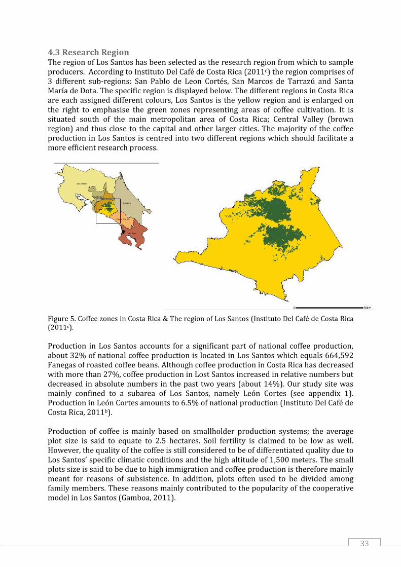
33

4.3 Research Region The region of Los Santos has been selected as the research region from which to sample producers. According to Instituto Del Café de Costa Rica (2011c) the region comprises of 3 different sub-regions: San Pablo de Leon Cortés, San Marcos de Tarrazú and Santa María de Dota. The specific region is displayed below. The different regions in Costa Rica are each assigned different colours, Los Santos is the yellow region and is enlarged on the right to emphasise the green zones representing areas of coffee cultivation. It is situated south of the main metropolitan area of Costa Rica; Central Valley (brown region) and thus close to the capital and other larger cities. The majority of the coffee production in Los Santos is centred into two different regions which should facilitate a more efficient research process. Figure 5. Coffee zones in Costa Rica & The region of Los Santos (Instituto Del Café de Costa Rica (2011c).

Production in Los Santos accounts for a significant part of national coffee production, about 32% of national coffee production is located in Los Santos which equals 664,592 Fanegas of roasted coffee beans. Although coffee production in Costa Rica has decreased with more than 27%, coffee production in Lost Santos increased in relative numbers but decreased in absolute numbers in the past two years (about 14%). Our study site was mainly confined to a subarea of Los Santos, namely León Cortes (see appendix 1). Production in León Cortes amounts to 6.5% of national production (Instituto Del Café de Costa Rica, 2011b). Production of coffee is mainly based on smallholder production systems; the average plot size is said to equate to 2.5 hectares. Soil fertility is claimed to be low as well. However, the quality of the coffee is still considered to be of differentiated quality due to Los Santos’ specific climatic conditions and the high altitude of 1,500 meters. The small plots size is said to be due to high immigration and coffee production is therefore mainly meant for reasons of subsistence. In addition, plots often used to be divided among family members. These reasons mainly contributed to the popularity of the cooperative model in Los Santos (Gamboa, 2011).

34

Besides discussing qualitative information retrieved from interview with experts; there is also quantitative information on coffee production. The census published on Costa Rica’s national coffee sector provides sufficient background information (Instituto Del Café de Costa Rica, 2007). The most relevant information for our region is displayed below in table 6. Table 6. Producer Characteristics Leon Cortes Hectares Quantity % Total Size % Credit Hire

Labour < 1 124 17% 62.1 1.1% 8.2% 31.5%

1 – 5 354 49% 884 15% 13.2% 47.2% 5 – 10 131 18% 914 15.5% 14% 63.4%

10 – 20 66 9.1% 895 15.2% 33.3% 81.8% 20 – 50 39 5.4% 1,194 20.3% 33.3% 94.9% 50 -100 8 1.1% 503 8.6% 12.5% 62.5%

> 100 6 0.8% 1,433 24.4% 16.7% 83.3% Total 728 100% 5,886 100% 18.3% 53.6%

Although the information in the report on León Cortes dates from data obtained in 2006, it is still worthwhile to discuss here. The report supports the information obtained from experts; almost half of the producers concern smallholders holding between 1 and 5 hectares only. Although large scale producers (more than 50 hectares) represent only 2% of the population they still hold 33% of the total land. This is again the opposite for smallholder producers. Receiving credit and the amount of hired labour is in line with what we commonly expect when comparing smallholders with large scale producers. It seems as that smallholders do not require credit or may not have access to credit. Whereas larger farmers apply or receive credit more often. The largest producers do not seem to be dependent of credit in their financial decisions. These findings suggest that opportunities to buy land for smallholders is limited. In addition, usage of hired labour is most prevalent with large scale producers; which makes perfect sense.

35

4.4 Value Chain In this section I will elaborate on the coffee value chain. The first part mainly comprises the chain itself, the different stages and the distribution of value added among its actors. Afterwards, the two main buyers which we have encountered will be discussed. They all possess different traits and both exert a unique impact on the value chain and primary producers.

4.4.1 The Coffee Value Chain The coffee chain can roughly be divided into 3 stages, 1) the growing and possibly initial processing on the farm, 2) processing and/or roasting and exporting within the producing country and 3) importing, further processing, roasting, the production of instant coffee and the sale in consumer countries. The first two stages generally reside in the production countries and are mainly controlled by individuals and smaller firms while the last stage is situated in consumer countries and is mainly controlled by (a few) large multinationals organizations (Talbot, 1997). Figure 6. Coffee Value Chain (Samper, 2010)

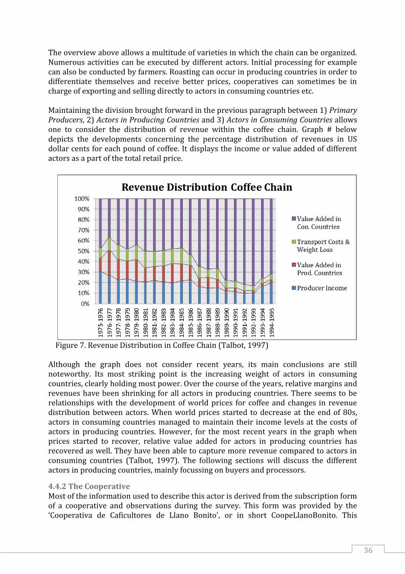
36

The overview above allows a multitude of varieties in which the chain can be organized. Numerous activities can be executed by different actors. Initial processing for example can also be conducted by farmers. Roasting can occur in producing countries in order to differentiate themselves and receive better prices, cooperatives can sometimes be in charge of exporting and selling directly to actors in consuming countries etc. Maintaining the division brought forward in the previous paragraph between 1) Primary Producers, 2) Actors in Producing Countries and 3) Actors in Consuming Countries allows one to consider the distribution of revenue within the coffee chain. Graph # below depicts the developments concerning the percentage distribution of revenues in US dollar cents for each pound of coffee. It displays the income or value added of different actors as a part of the total retail price.

Figure 7. Revenue Distribution in Coffee Chain (Talbot, 1997) Although the graph does not consider recent years, its main conclusions are still noteworthy. Its most striking point is the increasing weight of actors in consuming countries, clearly holding most power. Over the course of the years, relative margins and revenues have been shrinking for all actors in producing countries. There seems to be relationships with the development of world prices for coffee and changes in revenue distribution between actors. When world prices started to decrease at the end of 80s, actors in consuming countries managed to maintain their income levels at the costs of actors in producing countries. However, for the most recent years in the graph when prices started to recover, relative value added for actors in producing countries has recovered as well. They have been able to capture more revenue compared to actors in consuming countries (Talbot, 1997). The following sections will discuss the different actors in producing countries, mainly focussing on buyers and processors.

4.4.2 The Cooperative Most of the information used to describe this actor is derived from the subscription form of a cooperative and observations during the survey. This form was provided by the ‘Cooperativa de Caficultores de Llano Bonito’, or in short CoopeLlanoBonito. This

37

cooperative was found most common among the producers we have interviewed. The other two cooperatives include CoopeTarrazu and CoopeDota, of which both are located further away from the majority of the producers. It is often been brought forward that the cooperative is ‘for the community’ and that it represents ‘common interests’. Some even go as far as claiming that submitting to other firms than the cooperative can be seen as an act of treason. Transport costs, when choosing to which cooperative to sell, are assumed to play a minor roll since collection points are opened up during harvest in order to enable producers to submit coffee to other cooperatives while avoiding excessive transport costs. CoopeTarrazu for example has recently opened collection points in an area mostly served by CoopeLlanoBonito. The requirements which the cooperative enforces upon subscription include general demographic and economic information; Besides these key points, applicants also have to indicate whether they have been a member before and if so, why they have cancelled their membership. Moreover, membership also imposes the applicants to make a contribution to the cooperative’s ‘Social Capital’. Although this requirement was not specific on what this contribution relates to in detail. The document then needs to be signed by the administrative board, the cooperative president and the applicants himself. Most of the producers have been member for a significant amount of time already; on average 25 years for CoopeLlanoBonito. Producers have just recently started selling to other cooperatives; . about 6 and 2 years for CoopeTarrazu and CoopeDota respectively. Although the form is concise and relates to clear aspects which should be applied to each member, reality differs substantially. While the cooperative’s employees seem to be aware that producers oblige themselves to submitting a predetermined quantity of Fanegas, the majority of the producers (75-100%) themselves are hardly aware such a requisite even exists. But first of all, it seems as producers do not consider the subscription form to be a contract. It is always referred to as ‘Being a Member’. The cooperatives do put stringent demands on the quality of coffee beans which are submitted according to producers. They should be ripe, i.e. only include red coffee cherries, and not contain any leaves. Prices vary each year, cooperative seems to adjust them in association with the market price. Almost all of the producers received CRC (Costa Rican Colones) 100,000 for each Fanega. However, producers seem to be well aware of the extra services the cooperative provides, without the form having actually mentioned them. CoopeLlanoBonito does reasonably well with regards to offering technical assistance (prescribing pesticide mix, diagnosing plant diseases, taking soil samples), around 65% agree that technical assistance is available when necessary while an additional 32% agree that assistance is

Economic Information Place & size of the farm Area devoted to coffee production Areas devoted to other activities Coffee variety Number of Fanegas to be submitted

Demographic Information Applicants’ name Address Telephone number Date of birth Spouse’s name

38

available but limited (N=90). For CoopeTarrazu, these numbers amount to both 50% (N=18). CoopeDota however, fails to provide technical assistance; 50% claim they do not receive any assistance while the other 50% claim they do but there is limited availability (N = 4). With regards to prepayments, none of the cooperatives provide a payment before the harvest is actually delivered to a collection point. However, we only consider prepayments when no interest is charged. If one considers the type of loans that producers receive from cooperatives, there is a point to be made. Over 70% of the loans (N = 97) which coffee producers receive are received from cooperatives. The size of the loan is in 95% of the cases based on the harvest, land or another asset. In addition, the period of the loan rarely extends 8 months. Over 45% of the loans issued from cooperatives are shorter than 8 months. While even 85% of the loans are paid off within 12 months. These short term loans can be considered to ensure the availability of sufficient capital throughout the year and are based on the expected coffee harvest. Revenues from coffee production are received once every year. So it appears that producers are not able to balance their expenditures and income when they receive capital only once a year. The cooperative provides a certain ‘prepayment’ on their harvest but producers need to pay an interest rate. To conclude, the relationship between producers and cooperatives is a considerably close one. This is characterized as well by the provision of additional information amongst them. The term ‘additional information’ relates to non-ordinary information such as market behaviour, price developments etc. Information on market behaviour is sufficiently provided by the cooperative according to 78% of the producers. For ‘ordinary’ information, such as products norms and specification, 92% agree that the cooperative succeeds into communicating these well.

4.4.3 Diversified Buyers & Processors The other chain which is relevant to consider is where coffee is sold to a variety of buyers. These mainly include a cooperative and/or a private enterprise (e.g. Volcafe pertaining to Nespresso) and/or a microprocessor. Besides exploring general aspects about the producers pertaining to this chain, special focus is given to microprocessors. There is a modest amount of literature available on microprocessors in Costa Rica. In Spanish they are referred to as ‘Micro-beneficios’, which stands for small scale processors (while ‘common’ processors are referred to as just Beneficios). In response to the coffee crisis, farmers, processors and export firms realized that the impact on the coffee commodity chain would be permanent; processing and exporting became more concentrated while middle-sized and smallholder associations were setting up their own processing plants (i.e. micro-beneficios or micro-processing plants) in order to cope with short term difficulties and price fluctuations. The number of microprocessors has grown substantially; in the period 1999-2000 there were 94 plants registered at Icafe while in 2009-2010 this has grown to 161 plants. Although not all the microprocessors have submitted data on their production; the majority (57) over what is known relate to small scale processing amounting to less than 1,000 Fanegas. Another 21 plants process between 1,000 and 3,000 Fanegas (Barquero, 2011). Micro-processors integrated the production and processing stage; processing their own coffee and that of their neighbours. These farmer associations enabled themselves to

39

differentiate their coffee in terms of quality and thereby adding value (Samper, 2010). Farmers submitting coffee to these microprocessors can obtain up to $100 additional revenue per Fanega compared to mainstream channels applying world prices. They leave out exporters and sell directly to toasters and international markets. Processing involves removing fruit from the coffee beans and afterwards drying them. Farmers apply more careful methods during processing and likewise obtain a product that is more appreciated in international markets. Acquiring necessary equipment is a significant investment, however up to 30% is subsidised by different governmental organizations (Picado, 2010). The results obtained from the survey are mainly in line with the information which is discussed above. With regards to price differential due to quality attributes; producers submitting coffee to microprocessors do receive higher prices per Fanega. Microprocessors seem to value product quality more and producers accrue an additional price margin varying from 3% to an astonishing 100% compared to standard prices. Contrary to other buyers (e.g. cooperatives) microprocessors do not apply the same price to all producers. In addition, the relationship between the producers and microprocessors is quite loosely regulated and varies among different producers. The majority of the producers claim to have no agreement while the other majority argue that the relationship is limited to a ‘Verbal Agreement’ only. In most cases they have not agreed beforehand on the quantity, the quality on the other hand has been specified to the producers. None of the producers receive any technical assistance from the microprocessors.

40

5. Data Analysis This section will discuss general economics of coffee cultivation based on the information gathered during our survey. We will commence by exploring the economic situation of the farmers and afterwards we intend to relate our analyses with an environmental dimension. Values in Costa Rica Colones (CRC) have been converted into United State Dollars (USD = CRC 497.8449), applying the average exchange rate of the month (august) in which our survey was conducted6. In addition, we have converted the common land measurement unit ‘manzana’ in Costa Rica to hectares. One Hectare is roughly equal to 1.43 manzana7. The information on ‘Fanega’ has already been provided earlier; one Fanega contains 46 kg processed and dried coffee beans. Data has been processed using PASW Statistics 18.0 or formerly known as SPSS. The questionnaire can be found in appendix 3. The following section will discuss the most relevant descriptive statistics for a selection of variables and likewise summarize the most relevant topics that can be found back in our questionnaire. We will first provide an introductory overview on the coffee production while considering farm size, value chains and sustainability. Afterwards we will provide the main descriptive statistics on our sample. The last parts of section 5.1 will separately discuss several regression models using different variables.

5.1 Economics of Coffee Production We have already mentioned that coffee prices were at an unprecedented level; this might affect coffee farmers’ profitability. On average, coffee producers have witnessed a reasonably profitable year. Table 7. Division between Respondents on Size of Coffee Plots

We have applied a division with regards to the size of the farm based on the size of the coffee plots. Table 7 above displays the classes in hectares and below the number of respondents that e.g. hold between 0 and 0.99 hectares (15). We have applied a format

6 http://www.currency.me.uk/ 7 http://www.convertunits.com/

Coffee Plot Size (Ha.): 0 – 0.99 1 – 2.49 2.5 – 4.99 5 – 9.99 > 10 Overall

(N) : (15) (47) (23) (14) (5) (104) Revenue 3,919 13,171 20,385 46,608 67,283 20,535 - Inputs 891 2,412 4,056 8,509 17,191 4,088

Value Added 3,028 10,759 16,329 38,099 50,092 16,447 - Hired Labour (HL) 174 2,103 3,890 9,482 20,859 4,115 - Planting Trees 74 391 418 764 3,509 552

Gross Margin 2,780 8,265 12,021 27,853 25,724 11,780 - Family Labour (FL) 1,624 1,806 2,556 2,920 2,055 2,056

Return on Land & Other Assets

1,156 6,459 9,465 24,933 23,669 9,725

Size Coffee Plots (Ha.) 0.6 1.8 3.5 6.2 13.1 3.1 Costs / Hectare 3,870 3,756 3,314 3,578 3,260 3,627 Return / Hectare 3,521 3,352 2,891 4,222 1,815 3,318

41

that should explain the general situation on production economics. Naturally, the revenue on coffee production is higher with more hectares as well as the amount of hired labour. Although most averages such as the costs on family and hired labour, inputs, planting trees are of course more as farm size increases; total production costs per hectare are fairly similar. However, average profit per hectare is higher among smaller farmers. An explanation might relate to the more intensive land use among smaller farms; however it might also be due to the answers of the respondents themself. We have observed often that respondents tend downsize their land holdings; often replying that they holds less land than they actually do. This is mostly due to fear that information might end up in the wrong hands since producers do not pay taxes on profit and/or land holdings. Table 8. General Division between 1) Value Chains and 2) Sustainability

Table 8 elaborates on another division; between value chains and with regards to the degree of sustainability. There are 73 producers pertaining to the cooperative value chain and 31 producers for the diversified value chain. With regards to sustainability there are 82 conventional producers and 22 sustainable producers. We have applied the same format as Starbucks. They only include producers in their sustainability program if they are able to get 60% of the points which amounts to 24 points of a total of 40. The upper part, just as table 7, displays the format we have chosen in order to depict production economics while the bottom part considers average profit and total production costs per hectare. In this case we have only included average farm size in hectares as well. With regards to different value chains; the producers in the diversified value chain do seem to earn more on average. This is probably due to higher average land holdings and the price premium they face in the diversified chain. Overall, costs seem to be fairly similar on average. Although some numbers for the diversified chain are considerably different, this might be due to the inclusion of some large producers in this reasonably small group of respondents (only 31 respondents). Concerning sustainability, the number of respondents that have a score above 24 is rather small; only 22 so one can say that the same argument applies to this group. However, one can

1. Value Chains 2. Sustainability

(N) :

Cooperative 73

Diversified 31

Conventional 82

Sustainable 22

Revenue (Q * P) 17,974 26,564 17,524 31,756 - Inputs 3,515 5,435 3,512 6,233

Value Added 14,459 21,129 14,012 25,523 - Hired Labour (HL) 3,753 4,967 3,276 7,243 - Planting Trees 555 544 432 996

Gross Margin 10,151 15,618 10,304 17,284 - Family Labour (FL) 2,060 2,046 1,921 2,556

Return on Land & Other Assets

8,091 13,572 2,665 5,316

Size Coffee Plots (Ha.) 3.0 3.5 2.8 4.4 Costs / Hectare 3,560 3,691 3,561 3,875 Profit / Hectare 3,011 4,039 3,323 3,298

42

state that the average for this group are different with regards to farm size which impacts costs and profit as well. However, again the profit and total costs per hectare are similar for both conventional and sustainable producers. We will try to elaborate on the dynamics of coffee production more using mainly regressions that are meant to provide an overview on the contribution of various variables to production.

5.1.1. Farm Resources Farm resources include a.o. the amount hectare devoted to coffee production, the level of education and the number of family members. We assume the last variable might be correlated with the amount of contracted labour. Table 9 on the next page summarizes the main descriptive statistics for a selection of variables. The mean for the average education level is just over 4; which corresponds to having completed primary school. Other resources are displayed in monetary values. Input costs, labour costs, expenditures on new coffee plants and the expenditures on harvesting coffee are all in USD. Table 9. Descriptive Statistics on Research Sample

The information on costs has been divided into different sets. These deserve a short explanation, although we will elaborate on these variables in the following sections. The most relevant variables in terms of costs relates to the ‘Expenditures on Farm Inputs’. They consist of physical input (expressed in USD); namely fertilizer (both chemical and organic), herbicides, fungicides, pesticides, packaging material and transportation. Although costs on harvesting coffee are also considerable, they mainly refer to labour costs. In table 7 and 8 it has been added to hired/family labour but now it has been separated from ‘Total Labour Costs’. The variable on labour costs now consists of labour costs related to fertilization, manual weeding, applying herbicides, plague control,

Descriptive Statistics for Main Variables on Farm Resources

N Mean Std. Deviation Min Max

Total Size of Coffee Plots in Hectare (He)

104 3.1 2.9 0.2 16.8

Average Education for Household

104 4.0 1.1 1 6.8

Number Household Members

104 4.20 1.4 1 10

Total Labour Costs (USD)

104 2,087 2,384 99 18,118

Total Expenditures on Renewing Coffee Trees (USD)

104 552 1,112 0 9,525

Expenditures on Farm Inputs (USD)

104 4,088 4,439 56 27,981

Expenditures on Harvest Coffee (USD)

104 3,226 4,225 0 22,497

43

pruning and desuckering. During data collection, respondents were asked for the amount of labour days (both family and contracted) for each of these activities. Wages are fixed based on work per day; which equals approximately USD 11.05 per day8. Likewise labour costs were calculated, enabling us to differentiate between activities and family/contracted labour.

5.1.2. Multiple Regression Model on Coffee Production Considering the division in farm resources above can be worthwhile if one wants to examine a ‘straightforward’ production function. These resources hold characteristics that should affect e.g. production. Several hypotheses can be formulated: H1 Land has a significant and positive affect on the production of coffee. H2 Resources such as physical input (i.e. ‘Expenditures on Farm Input) and to a

lesser extent ‘Total Labour Costs’ hold a significant and positive affect on production.

H3 The expenditures on planting new coffee trees do not hold any significant effect on the production of coffee.

H4 Coffee plant age and the number of plants per hectare should significantly contribute to production.

Regression analysis lends itself very well for examining these hypotheses. The essence of regression analysis is predicting an outcome variable (Coffee Harvest in Fanegas) from one or more independent variables. We believe a Cobb-Douglas production reflects the production of coffee best instead of a straightforward linear production function. The relation between inputs and the output is assumed to be a non-linear one. This can be modelled by converting the variables into their natural logarithms. The resulting regression coefficients can then be interpreted as elasticities. They will indicate the percentage change in production due to a one percent increase in the input (Tintner & Brownlee, 1944). According to Field (2009) the outcome one is trying to predict for a specific situation can be predicted by applying a model plus some kind of error. In our case this would represent the following Cobb-Douglas production function: (1) (2) The second formula is the same as the first formula however it is converted to natural logarithms. The parameters used in the formula above are known as regression coefficients and they represent the following: Υi Outcome for each respondent ‘i’ Ci The constant associated with respondent ‘i’ Βij The regression coefficient / elasticity for each respondent ‘i’ for each variable ‘j’

associated with the variable Xij. In multiple regressions, more variables are introduced and as a consequence the formula will contain more regression coefficient that refer to the elasticity associated

8 In Costa Rica they are referred to as ‘Jornal’ and relate to CRC 5,500 per day.

44

with different variables. In our case the variables associated with the different regression coefficients refer to the following: X1 Size of coffee plots in hectare X2 Expenditures on Farm Inputs X3 Total Labour Costs X4 Expenditures on Planting New Coffee Trees X5 Average Education for Households X6 Sustainability Score X7 Number of Plants per Hectare X8 Average Age of Plants The reasons for including these specific variables are rather straightforward; these are basic and typical inputs in production, traits of coffee plots and household characteristics which are assumed to impact levels of production. The final aim is to come up with an appropriate model in terms of goodness in which we are able to incorporate and examine variables regarding sustainability. Land is a rather logical variable to include, however the model might face difficulties analysing labour costs and expenditures on physical inputs since they might correlate considerably. This also applies to land of course. We assume the educational level might effect the use of resources; a more efficient one namely which might be reflected in increasing production. Finally the number of plants per hectare also holds a non-linear relationship with production levels; there is only room for a limited amount and an additional unit of coffee plants does not lead to an equal increase in units of output. The average age of plants/coffee trees should also hold a positive relationship; they become productive only after 2-3 years and older coffee trees might produce more. Producers and experts however, tend to differ in their opinion on the productive life of coffee trees. Conducting this multiple regression using the variables mentioned above in SPSS leads the results displayed in table 10 on the next page (Model 1. General Model). The output files can be found in appendix 4.1. For the sake of clarity, we have compiled the different regression model in one table. We will discuss the proceeding models separately. A noteworthy piece of information refers to what is called ‘R Square’ / R2 which represents the amount of variance9 in the outcome explained by the model relative to how much variation there was to explain in the first place (bottom of the table). To conclude, our model is able to explain almost 75% of the variance found in our dataset. Another important part is the F-ratio10 and its associated significance value. For our data F equals 32.48 which is significant at ρ < 0.01. This means that there is less than a 0.1% chance that we will came across an F-ratio this large. Now we can elaborate on the hypothesis we have set earlier. The coefficients for land and expenditures on physical inputs are significant. Therefore H1 can be confirmed. Land seems to be the most relevant aspects, reflected by the high elasticity of land (0.44). Expenditures on input have a smaller elasticity; keeping land constant and applying more fertilizer might let it become ‘saturated’ since applying 1% more fertilizer only leads to 0.26% additional harvest. Although the same applies for land, the elasticity (0.44%) is not that low.

9 Variance refers to an estimate of average variability of a set of data (Field, 2009)

10 A ratio of the average variability that a model can explain to the average variability unexplained by the same

model (Fields, 2009).

45

Table. 10 Regression Models

* ⍴ < 0.10, ** ⍴ < 0.05 & *** ⍴ < 0.01. Dependent Variable: Ln(Harvest in Fanegas)

Model 1. General Model

Model 2. ‘Unfolded’ Input Variables

Model 3. ‘Unfolded’ Input & Labour Variables

Model 4. Sustainable Practices

Variables N:

B – Coeff. SE B 94

B – Coeff. SE B 94

B – Coeff. SE B 94

B – Coeff. SE B 94

Constant - 1.38 1.41 - 9.11 4.61 -2.88 1.68 -1.27 1.44

Ln(Coffee Plot Size) 0.44*** 0.14 0.38*** 0.13 0.33** 0.14 0.43*** 0.14

Ln(Expenditures Inputs) 0.26*** 0.10 0.30*** 0.11 0.32** 0.11 0.28*** 0.10

Ln(Total Labour Costs) 0.10 0.09 0.15 0.10 0.17 0.11 0.08 0.10

Ln(Expenditures Planting) -0.01 0.02 -0.01 0.02 -0.01 0.02 -0.009 0.02

Household Education 0.01 0.05 -0.003 0.05 -0.003 0.05 -0.002 0.05

Ln(Sustainability Score) -0.02 0.17 0.10 0.17 -0.06 0.17

Plant Age 0.003** 0.001 0.003* 0.001 0.003* 0.001 0.004** 0.002

Ln(Plants per Hectare) 0.29* 0.17 0.38** 0.16 0.33* 0.18 0.26 0.17

Ratio Chemical Fertilizer 6.46 4.10

Ratio Organic Fertilizer 6.58 4.12

Ratio Herbicides 11.11* 5.73 -0.46 3.78

Ratio Insecticides 3.83 4.71

Ratio Fungicides 4.42 4.29

Ratio Transportation 6.16 4.13

Ratio Lab. Costs Fertilization

1.11 0.82

Ratio Lab. Costs Herbicides 0.17 10.01

Ratio Lab. Costs Weeding Excluded by SPSS

Ratio Lab. Costs Plague Control

-0.21 0.44

Ratio Lab. Costs Pruning 1.41* 0,76

Ratio Lab. Costs Desucker 0.84 0.61

Bench Terraces 0.06 0.11

Individual Terraces -0.16 0.15

Costs Registration -0.04 0.11

Organic Fertilizers -0.008 0.11

Diversion Canals 0.14 0.15

Exit Canals 0.03 0.10

Model adjusted R2 0.73 0.75 0.74 0.72

F - Statistic 32.48*** 21.17*** 19.77*** 19.89***

46

Referring to H2, we can only partly confirm this; only physical inputs seem to contribute significantly to harvest in Fanegas. That might be related to labour and land being correlated; cultivating more land requires more labour as well. It is likely that labour is ‘hidden’ in the information on land, therefore it is not significant in the model. Moreover, average educational level does not seem to contribute to the harvest in Fanegas. In our third hypothesis H3 we argue that investments in new plants hold a significant negative effect on harvest. We assumed, since coffee plants take 3 years before they start producing coffee cherries, that there is no significant relationship. The expenditures on new plants concern this year. However, there is no significant negative relationship. We believed the coefficient to be negative due to the effects of recently planted coffee trees on existing and productive coffee trees; the new ones occupy land as well and likewise might extract nutrients from the soil at the costs of productive trees. Finally, the variables dealing with the number of plants per hectare and their age contributes to the model as well. The fourth hypothesis we have set can be confirmed; age and density of coffee plots significantly and positively effect production.

5.1.3. Expenditures on Input & Labour With regards to the previous section, separating and examining several activities within a larger set might be worthwhile for examining the individual contribution of separate input variables. While focussing on model 1 (‘General Model’) but this time including the ratios for the types of physical inputs can clarify whether e.g. chemical fertilizer or herbicides make any significant contribution to harvest. For example the application of pesticides on the other hand can indicate the occurrence of harsh pests in coffee plots which might again indicate a downfall in production. They are not variables converted to their natural logarithms but rather the ratio of the total expenditures on input. Their corresponding significance value shows whether they make a significant contribution to harvest. With regards to the overall fit of the model; we have achieved similar variance. As can be seen from the information below the column labelled ‘Model 2 Unfolded Input Variables’ (Appendix 4.2) in table 10, R2 equals 0.79 so only 21% is left unexplained. The corresponding F-ratio however is considerably smaller and equal to 21.27. Results brought forward by this model are similar to the first model; land and inputs are significant and hold similar elasticities. However, none of the ratios associated with specific input types are significant. The model does not seem to succeed in clarifying individual contributions. Which is remarkable; one would assume a strong relationship between at least chemical fertilizer and harvest. Neither are we able to examine whether the use of pesticides indicates a downfall in production that is possibly associated with the occurrence of pests. The third model (see appendix 4.3) in table 10 labelled ‘Unfolded Labour Variables’ shows similar results as the second model (‘Unfolded Input Variables’). We have incorporated the variable that showed a significant coefficient in model 2 namely expenditures on herbicides (although only at the 0.10 significance level) in model 3 as well. However, the third model does not provide additional significant results. SPSS does not seem to be statistically able to calculate the ratio on weeding costs and the ratio on herbicides is not significant anymore.

47

5.1.4. Conclusive Note on Regression Models The non-linear regression models we have presented here are rather similar in its outcome and goodness of fit. The variables on physical input and land remain significant regardless of the model, however only discussing inputs is not sufficient. Considering labour costs as well does not lead to a more complete overview. Moreover, throughout the different models the effect of plant age is also demonstrated. Higher plant age leads to a higher production levels. This effect is more prevalent for the number of coffee trees per hectare, although in the last model we did not witness significant results for this variable. Still in the first three models, the variable on coffee trees per hectare has a high elasticity; mostly around 0.30-0.35. The first model ‘General Model’ remains the preferred one; it clarifies the decreasing marginal returns for physical inputs, number and age of coffee trees and land. The second and third model have not succeeded into coming up with a clearer overview on the contribution of the different variables within the overall variable on labour and physical inputs.

5.2 Incorporating an Environmental Dimension in Production The previous section has tried to elaborate on the dynamics that can be found in the economics of coffee production. However, we have not yet addressed the environmental dimension within coffee production. Earlier in section 2.3.4., we have discussed studies that investigate sustainable production, its characteristics, determinants and consequences. In addition, we have explained our producer ranking with regards to sustainable methods in section 3.2. The associated score lends itself well when assessing several traits with regards to sustainability. An aspect we have not discussed yet in the previous section, but which has been incorporated in model 1, 2 and 3, is the sustainability score and its relationship with production levels. The natural logarithm of the sustainability score is also incorporated in models 1, 2 and 3 in table 10. None of the models indicate a significant relationship between sustainability and production. However, since the sustainability score we have computed is based on a range of sustainable practices, combining all these practices and addressing them in one overall score might overlook the impact of specific practices. Model 4 (‘Sustainable Practices’) in table 10 omitted the variable on sustainability but instead incorporated several dummy variables on specific practices (see appendix 4.4 for output files). We have focussed on the effects of individual and bench terraces, registration of costs/revenues, application of organic fertilizers, exit canals and diversion canals. We assume that applying terraces is an effective strategy in order to reduce the slope of coffee plots which again should reduce soil erosion and its impacts. Moreover, since certification programs such as Fair-trade and Starbucks also incorporate management requirements into their set of standards, we also decided to focus on the registration of costs/revenues. Organic fertilizers is believed to improve nutrient levels and diversion and exit canals both reduce the risk of erosion as well by limiting the impact of rainwater to the soil. However, yet again none of these variables are significantly associated with production.

5.2.1. Exploring the Degree of Sustainability Elaborating on the relationship between specific variables and the degree of sustainability allows us to investigate different characteristics on sustainable producers. A method which lends itself well is examining the correlation coefficient as a first step. The most well-known correlation coefficients is called the Pearson correlation

48

coefficient. The coefficient informs on the relationship that two different variables hold to each other; a coefficient of +1 would suggest a perfect correlation. Increasing one variable would results in a proportionate increase of the other variable. The same applies to a coefficient of -1 but vice versa. If the size of the effect (correlation coefficient) corresponds the a value of ± 0.1 it represents a small effect, ±0.3 stands for a medium effect and ±0.5 represents a large effect (Field, 2009). However, it assumes normality in the sample. Likewise, we first need to examine the distribution of the variables before in order to select an appropriate method. Appendix 4.7 displays the results of the Kolmogorov-Smirnov test. This test compares the scores in the sample with a normally distributed score that has the same mean and standard deviation. If the test is significant (ρ > 0.05) it tells us that the distribution of the sample is significantly different from a normal distribution (Field, 2009). All the variables are significant (ρ > 0.001); they differ significantly from a normal distribution. Considering the paragraph above, non-parametric statistics are more relevant since they do not rely on a normal distribution but on ranking the respondents. The most suitable and apparently better non-parametric estimate of the correlation coefficient is the Kendall’s Tau statistic; especially useful when dealing with small sample size and a large number of tied ranks. Appendix 4.8 elaborates on the Kendall’s Tau correlation coefficients for a selection of variables in order to explore the relationship with the degree of sustainability. The correlation coefficients corresponding with our variables on labour costs per hectare and total labour both show medium effects. The coefficient for total labour is significant and equals -0.22 and the coefficients for labour costs per hectare is somewhat smaller at -0.16. We have gained more insight by considering each specific labour activity; only labour costs for fertilization and pruning seem to significantly relate to our degree of sustainability. The corresponding correlation coefficients on the labour costs per hectare for fertilization and pruning are negatively correlated with sustainability; -0.16 and -0.17 respectively. In addition, costs on a labour activity which comes close to ‘significance’ level relates to manual weeding; ascending one place in the overall ranking for sustainability (i.e. less sustainable) relates to a decrease of costs on manual weeding equating to $ 0.13 per hectare (ρ = 0.05). Moreover, a practice that is again associated with sustainable agriculture has also been considered. The amount of organic fertilizer a producer spends per hectare is confirming our sustainability score as well. There is a significant and negative correlation of – 0.23 with the degree of sustainability. Again similar to the statement made in section 5.2, there is no significant correlation between expenditures in organic fertilizer and productivity per hectare. Neither does our degree of sustainability reflect any significant relationship with productivity per hectare (appendix 4.9). None of the other inputs are significantly correlated with our degree of sustainability It is affirming for our sustainability score that we have encountered relationships with activities associated with sustainable agriculture while the ones that are more harmful to environment are not significantly associated with our score for sustainability (Sustainable Agricultural Standards, 2010).

49

One can conclude that these results are consistent with the information we have discussed in previous sections. Furthermore, it increases credibility with regards to our degree of sustainability we have incorporated into our survey. These results we have put forwards in this section have modestly succeeded into clarifying interesting characteristics on sustainable producers. While there is no production gain, sustainable producers do tend to differentiate themselves from other ‘conventional’ producers with regards to the level of education and the higher amount of resources they devote to labour activities such as pruning, (organic) fertilization and to a lesser extent manual weeding. However, more rigid and thorough analysis is required if we are to address this issue better.

5.2.2. Characteristics of Sustainable Producers We can also look at it differently. Instead of examining whether sustainability correlates with the level of production and other variables, like we did in the previous paragraph, we can also investigate what contributes to sustainability. What variables tend to affect the degree of sustainability in one’s production system and how does the degree of sustainability affects coffee production? We intend to incorporate variables on resource availability and family endowments. We have come up with the following hypotheses: H5 The educational level of families will have a significant and positive effect on the

level of sustainability. H6 The amount of labour availability, measured by the number of family members,

will have a positive and significant effect on sustainability. H7 More sustainable producer will face increasing labour costs measured by labour

intensity/total labour costs and labour costs devoted to specific activities. H8 Higher degree of sustainability is associated with less intensive production and

longer productive life of coffee trees Running the regression analysis yield the results that are displayed in table 11 (see also appendix 4.6). The model itself does a poor job with regards to explaining the variance found in our sustainability scores; the corresponding R2 equals only 0.19. That means we are able to explain 19% of the variance in our sustainability score. The F-ratio equals 1.92 and it is significant (ρ < 0.05). The model might however still provide some explorative insights on the relationship between some variables and the degree of sustainability. Most of the analysis we set forward in this section relates to our first research questions, they all elaborate on the characteristics of sustainable producers. With regards to the hypotheses, the fourth one can be confirmed. The educational level does reflect a positive and significant relationship (ρ < 0.05). Labour costs per hectare on all of the activities and total labour costs per hectare are not associated with sustainability. The amount of labour availability does not reflect any significant relationship with the degree of sustainability (ρ > 0.05). We can reject both our fifth and sixth hypothesis. Labour availability does not show a relationship with the degree of sustainability and neither do labour costs per hectare. The seventh hypothesis is motivated by the belief that sustainable producers or production does not emphasise intensive production, as is reflected by the amount of coffee trees per hectare. We believed that a higher degree of sustainability is related to decreasing number of coffee trees per hectare. In addition, we also assumed that sustainable production increases productive life of coffee trees or

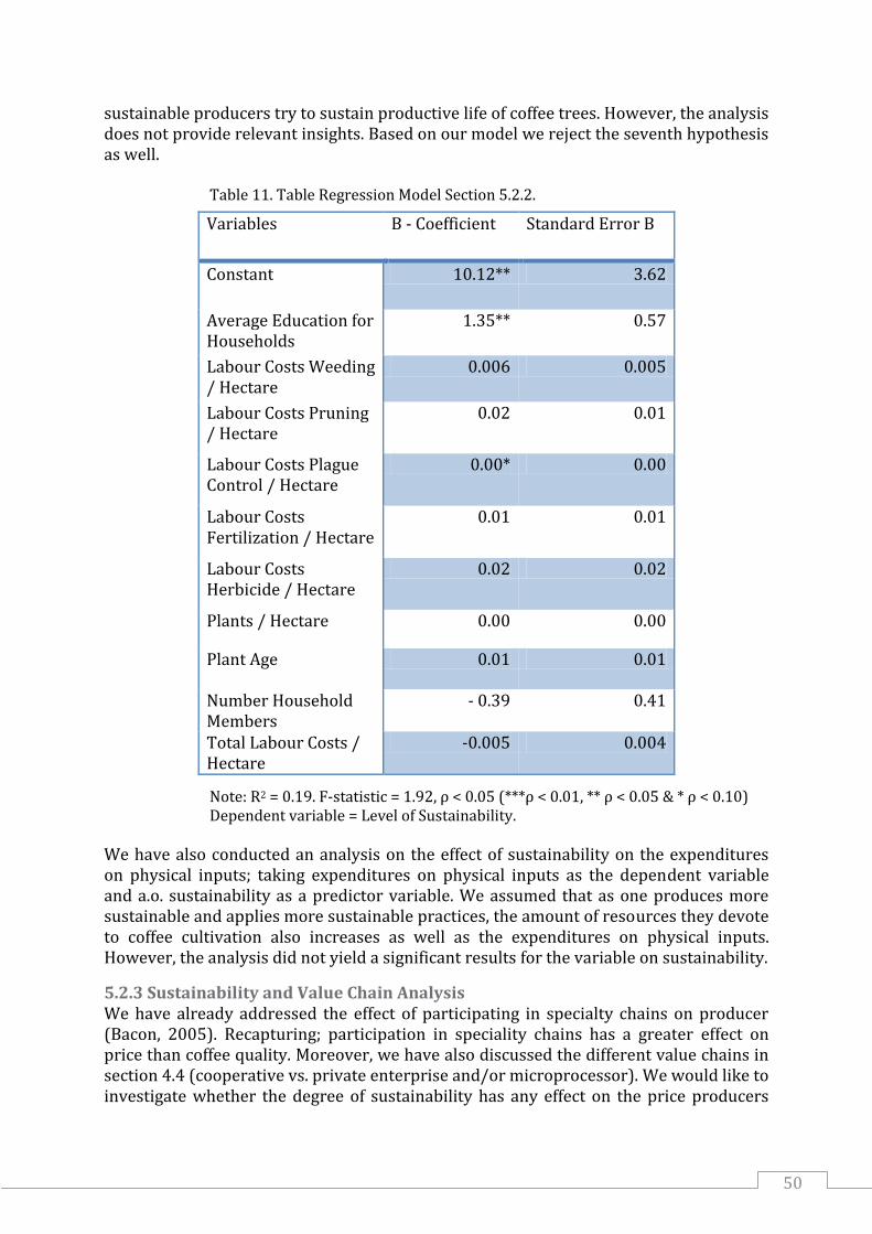
50

sustainable producers try to sustain productive life of coffee trees. However, the analysis does not provide relevant insights. Based on our model we reject the seventh hypothesis as well. Table 11. Table Regression Model Section 5.2.2.

Note: R2 = 0.19. F-statistic = 1.92, ρ < 0.05 (***ρ < 0.01, ** ρ < 0.05 & * ρ < 0.10) Dependent variable = Level of Sustainability.

We have also conducted an analysis on the effect of sustainability on the expenditures on physical inputs; taking expenditures on physical inputs as the dependent variable and a.o. sustainability as a predictor variable. We assumed that as one produces more sustainable and applies more sustainable practices, the amount of resources they devote to coffee cultivation also increases as well as the expenditures on physical inputs. However, the analysis did not yield a significant results for the variable on sustainability.

5.2.3 Sustainability and Value Chain Analysis We have already addressed the effect of participating in specialty chains on producer (Bacon, 2005). Recapturing; participation in speciality chains has a greater effect on price than coffee quality. Moreover, we have also discussed the different value chains in section 4.4 (cooperative vs. private enterprise and/or microprocessor). We would like to investigate whether the degree of sustainability has any effect on the price producers

Variables B - Coefficient Standard Error B

Constant 10.12** 3.62

Average Education for Households

1.35** 0.57

Labour Costs Weeding / Hectare

0.006 0.005

Labour Costs Pruning / Hectare

0.02 0.01

Labour Costs Plague Control / Hectare

0.00* 0.00

Labour Costs Fertilization / Hectare

0.01 0.01

Labour Costs Herbicide / Hectare

0.02 0.02

Plants / Hectare 0.00 0.00

Plant Age 0.01 0.01

Number Household Members

- 0.39 0.41

Total Labour Costs / Hectare

-0.005 0.004

51

receive and the participation in speciality chains. Our expectations (based on the article by Bacon, 2005) are represented in the following hypothesis. H9 Participation in speciality chains has a positive and significant effect on the

average price per Fanega for producers. H10 the degree of sustainability does not have a significant effect on price per Fanega

for producer or the participation in speciality chains. The first hypothesis is rather straightforward; selling to various buyers and also microprocessors should lead to higher prices that producers receive. Often producer sell a part of their coffee to private enterprises that are trying to acquire foothold in the market and they are often willing to pay higher prices. In addition, selling to micro-processors has already been related to higher prices as well since producers can differentiate their coffee and sell more directly to customers in consuming countries. With regards to the second hypothesis; the degree of sustainability in our case is not associated with certification. To be more precise, our sample does not involve certified and non-certified producers; we are focussing on (sustainable) production methods irrelevant of the inclusion of certification during production. Therefore we do not expect a relation between the degree of sustainability and price per Fanega nor the participation in speciality chains. In this case, we displayed the SPSS output below since it concerns a rather small table. We performed a non-parametric correlation method as we have done as well in previous paragraphs. As you can see, there is significant and positive correlation between the number of buyers as a measure of the participation in speciality chains and the average price per Fanega (ρ < 0.01). We can confirm our first hypothesis. However as we expected, there is no significant correlation between sustainability and average price per Fanega or participation in speciality chains. This is in line with our second hypothesis. Table 12. Kendall’s Tau Correlation Section 5.2.3.

Kendall’s Tau Correlation

Rank Sustainability (N)

Number of Buyers (N)

Average Price per Fanega (N)

Rank Sustainability - 0.00 (104) 0.043 (104)

Number of Buyers

0.00 (104) - 0.395* (104)

Average Price per Fanega

0.043 (104) 0.395* (104) -

* Correlation is significant at the 0.01 level (2-tailed) Besides conducting this exploratory analysis on correlation, there are also other methods available in order to examine what makes producers decide to opt for a specific chain. Logistic regression in this case would be suitable; the outcome or dependent variable in this case ought to be a categorical (or binary) variable instead of a continues variable as in the previous section (i.e. variable on harvest). With binary logistic regression we are able to predict the likelihood of a respondent being in a specific category while considering certain information (Hair et al., 2010). More specifically we would like to find out the probability for producers belonging to e.g. the diversified

52

chain in case they are more sustainable than other producers. We have inserted the most relevant information in table 13 below. Overall the model represents a good fit, the chi-square statistic (42.25) is significant (⍴ < 0.01). The R2 suggests that there is considerable improvement as a result of the inclusion of the predictor variables; 1 stands for the model predicting the outcome variable perfectly while 0 means the predictors are not contributing at all. In our case 0.66 is a considerable improvement. This is in line with the other coefficients which can be interpreted similarly (Cox & Snell, Nagelkerke). Table 13. Table Logistic Regression Model Section 5.4.3.

R2 = 0.66 (Hosmer & Lemeshow), 0.34 (Cox & Snell), 0.48 (Nagelkerke). Model X2 = 42.3, ⍴ <.01. *⍴ < .01

With regards to our selection of predictor variables, only one is significant. It seems producers only participate in this diversified value chain due to the price differential. The average price per Fanega is the only significant variable. We can argue that, considering the ‘Odds Ratio’, a producer who sells his coffee to a diversified value chain has an odd that is 1.29 times higher that he receives a better price per Fanega than producers who only focus on the ‘cooperative value chain’. The confidence interval for this variable is also beneficial, moving from an lower to an upper interval it does not cross 1 (1.13 to an interval of 1.47). The others do not make significant contributions. Neither does the level of sustainability; there is again no relation with the degree of sustainability and the likelihood of a producer entering a diversified value chain. One can say that there is no significant relationship between sustainable producers and the likelihood of opting for a diversified value chain. This also applies to the age of the household head and a family’s educational level. The analyses in the previous paragraphs mostly concern our second research questions, the following part is also in line with its main conclusions. Due to this section’s focus on sustainability especially we have performed a Mann-Whitney test, which is suitable for non-parametric variables, on the two groups of producers focussing on the two value chains and testing whether the ranks in the two groups is significantly different. We can conclude from this test that sustainability levels among producers in diversified value

95% Confidence Intervals for Odds Ratio

Variables B (SE) Lower Odds Ratio Upper Constant - 52.18* (13.86) - - -

Level of Sustainability

- 0.02 (0.05) 0.89 0.98 1.08

Age of Household Head

- 0.01 (0.03) 0.94 0.99 1.04

Average Price per Fanega

0.25* (0.07) 1.13 1.29 1.47

Average Household Education

0.16 (0.28) 0.68 1.17 2.02

53

chains (mean rank = 53.73) in different value chains do not differ significantly (⍴ > 0.05) from sustainability levels in the cooperative value chain (mean rank = 51.98).

5.2.4. Coffee Producers and Environmental Services This part focuses especially on the last research question. We have enquired among producers to the reasons why they would like to produce sustainable or more specifically why they tend to incorporate specific sustainable practices (e.g. shadow provision, limiting pesticide use etc.). It proved to be difficult answering that question for the majority of producers; often coming up with repetitive responses, they reverted to the question or avoided direct answers (.e.g. ‘because it is good for the environment’). Research has indicated that the attitudes and beliefs farmers hold with regards to either sustainable or conventional agriculture is an unconscious and diverse dimension. It requires elaborated techniques in order to let opinions on sustainable agriculture resurface. To conclude, their opinion or motivations for sustainable agriculture is often influenced by underlying values and beliefs and require specific paradigms in order to examine these notions effectively among producers (Comer et al., 2009). We have investigated only on the reasons which have provided us a very basic view on the motivations of producers. Therefore we are not able to answer the final research question well. We will limit ourselves in that case only to discussing the main reasons that producers brought forward. Most producers are quite consistently motivated, meaning that independent of specific circumstances they will keep caring for the environment. Very few producers agree that production volume or the price of pesticides influences them for conserving of the environment (N = 100). All but one (99%) producer claimed that they will not use more pesticides and keep conserving the environment the way they do already regardless of the price of pesticides. The production volume shows similar information; almost 92% claim that they will keep protecting the environment also if production volume deviates. Only 8% argue that they will protect the environment differently; either more conservation or less. The effect on the conservation of the environment seems to matter most in case of soil fertility and the chance of erosion. In case of low erosion and high soil fertility, almost 73% claim that they would not change their conservation efforts. However, 26% claim that they would put less effort into conserving the environment. This is the other way around in case of low fertility and high chances of erosion. According to a small share of the producers their conservation efforts seem to deviate due to fertility and the likelihood of erosion. The coffee price is the last determinant we have asked the producers; 85% will not change conservation efforts regardless of price. About 15% of the producers state that a good price allows them to conserve the environment more. This is again the other way around; in case of a bad coffee price they believe that they would likely conserve the environment less than they did before. To summarize, although we cannot statically indicate significant results on determinants for motivation it seems that at least a share of the producers believe that erosion/soil fertility is most important followed by coffee prices. Considering table 14 on the next page that summarizes the most prevalent reasons among our sample we can argue that the most popular reasons are similar to the statement made in the previous paragraph. Producers were asked, by posing open questions, what benefits they pursue or relate to sustainable production or sustainability in general. Depending on the number of benefits they would mention (maximum is 4), we attached a weight to each benefit. Mentioning only ‘Soil Fertility’

54

and ‘Improve Health’ would correspond to each benefit acquiring 0.5 points. We have done so for 103 respondents who were able to come up with at least one benefit. Producers found it increasingly difficult to come up with more than one reasons and, there are fewer producers that could come up with 3 or 4 different reasons for conserving the environment. Clearly, soil fertility and conservation are most frequently mentioned benefits. Other benefits related mainly to plant health, product quality while the rest of the benefits mainly relate to improved or more economical production. Table 14. Summary Sustainable Production Benefits Section 5.4.4.

In addition we have also enquired whether they could identify benefits that the community at large could receive if they would incorporate more sustainable production methods. They do seem to be able to separate benefits derived from production and benefits that can be received by the community. Clean water and fresh air are often associated and interpreted as possible benefits for the community. Another common answer include a vague one; namely ‘Conserving the Environment’ or ‘No Contamination’. Usually when producers were not able to come up with an answer they ‘circulated’ back to the questions by stating that there is ‘No Contamination’ / ‘Conserve Environment’. Other benefits relate to the improvement of health,

Benefits For Producers For Community Soil Conservation 19.7 % 2.2 % Soil Fertility 16.3 % - Plant Health 9.9 % 0.4 % Improve Product Quality 8.5 % 2.6 % No Contamination / Conserve Environment

8.0 % 19.2 %

Improved Production 6.5 % 0.4 % Improve Health 5.8 % 12.7 % Fresh Air 4.9 % 22.2 % Economical Production 4.8 % 2.8 % Animal Diversity 3.0 % 3.1 % Clean Water 2.5 % 15.9 % Improve Ecosystem & Nature 2.1 % 4.1 % Revert Global Warming 1.7 % 0.4 % Less Plagues 1.7 % 1.1 % Higher Food Availability 1.1 % 5.3 % Food Provision for Animals 1.1 % 1.7 % More Vegetation 0.8 % - Better Marketing / Price 0.5 % - Being Human 0.3 % - Equilibrium with Nature 0.2 % - Future Generations 0.2 % - Efficient Management 0.2 % - Source of Employment 0.2 % 4.2 % Snowball Effect of Positive Behaviour / Setting Example

- 1.9 %

55

5.3. Credit The opportunity to acquire a loan has also been investigated during our survey. We have enquired whether respondents have made use of credit, its terms, the source and if they would have liked to lend more money. In our sample, slightly over 65% have made use of credit during the last 3 years. If respondents acquired more than 1 loan in the past 3 years, a code was assigned to each specific loan. About 31% of the respondents have acquired 2 loans from different sources while only 4.8% (5 respondents) has received 3 loans from different sources/institutions. The majority (72%) of the loans were given out by coffee cooperatives. Only 16.5% are acquired from private or governmental banks, 5.2% from private enterprises while the residual relates to loans from NGO, Icafe and ‘Others’. The type of guarantee required by source mainly relate to land or a derivative of land (e.g. last year’s harvest); 92% of the loans require ‘land’ as a security measure or base the size of the loan on land holdings. The majority of the loans are paid back within a year; 77% has a term shorter than 12 months. The other 23% of the loans’ term vary between 2.5 years and 12 years; the largest group (9%) within the remaining 23% consists of loans concerns loans that need to paid back within 5 years. Non parametric tests involve ranking the respondents; we have done so based on the size of each individual loan. In case respondents have the same loan-sizes (i.e. a lot of tied ranks) the potential ranks are summed up and divided by the number of respondents holding that same score. For example; 2 loans equal in size of $16,070 with a potential ranking of 97 and 98 now both hold an actual rank 97.5. The output for the Kendall’s Tau correlation is similar to the output of the Pearson’s correlation. Table 15. Kendall’s Tau Correlation Section 5.3

*Correlation is significant at the 0.01 level (2-tailed) Conducting this analysis yields the results displayed in table 15 displayed. There is a significant correlation between the size of each individual loan and the quantity harvested and size of a producers’ land holdings, their correlations are 0.34 and 0.46 respectively and they are all significant.

Kendall’s Tau Correlation

Rank Loan Size (N)

Size Coffee Plots (N)

Income Enterprise (N)

Total Coffee Harvest (N)

Household Income (N)

Rank Loan Size

- 0.46 * (97)

0.26 * (97)

0.34 * (97)

0.36 * (97)

Size Coffee Plots

0.46 * (133)

- 0.19 * (133)

0.65 * (133)

0.50 * (133)

Income Enterprise

0.26 * (97)

0.19 * (133)*

- 0.04 (133)

0.19 * (133)

Total Coffee Harvest

0.34 * (97)

0.65 * (133)

0,035 (133)

- 0.62 * (133)

Total Household Income

0.36 * (97)

0.50 * (133)

0.19 * (133)

0.62 * (133)

-

56

Moreover, the output seems to suggest that income derived from business other than agriculture also seem to improve access to loans (especially the amount one can borrow). However, the income derived from other business’ is also correlated with land holdings and harvest quantity, as well the variables addressing a household’s total income (profit from coffee production + income salary worker + Income other business’). Land holdings and/or harvest quantity both affect loan size and income from other businesses. Conducting partial correlation might resolve this issue; controlling for land holdings and harvest size. The results can be found in appendix 4.4. Keeping land holdings and harvest size fixed still yields a significant correlation coefficient (ρ < 0.013) between income derived from enterprises and loan size. The results for household income do not hold; there is not a significant correlation coefficient (ρ < 0.094).

5.4. Off-Farm Income Acquiring information on off-farm income has also been conducted among our respondents. Food security is strongly associated with involvement in off-farm activities. In addition, income derived from off-farm activities enables farmers to increase agricultural yield by investing more in external inputs and it is able to increase labour productivity (Ruben & van den Berg, 2001). Diversifying household income can also cause more rapid growth with regards to earnings and household consumption (Barrett et al., 2001). We have considered 2 different sources of non-farm income; wage labourers and non-farm enterprises. In our sample about 36.5% of the household acquire income working as labourers on other (mainly coffee) farms. While only 13% acquire income derived from other business than coffee cultivation. Type of business is mainly related to trade (44%) while beekeeping comprises the second most common business (17%). Other important activities include retailing and craft (both 11%). Others mainly relate to tourism and the sale of agricultural inputs. With regards to wage labour, the most common relates to ‘Agricultural Worker’ (38%). Construction is the second popular (19%); that is probably due to the construction of a dam in the region for which the project employed labour from the region as well. Food processing (13%) mainly refers to being temporary employed be the cooperative during the harvest season. On average, households earn about $5,450 from wage labour per year and this concerns 48% of their total household income. Households that earn income derived from nonfarm enterprises earn almost $20,000 on average per year. However, almost 70% of the household focussing on nonfarm enterprises earn up to approximately $8,400 per year.

57

6. Conclusion Significant correlation coefficients, often related to the production process itself, were in line with basic characteristics on agricultural production. It enabled us to decide what relevant variables to include. Conducting multiple regression analysis revealed the contribution of several variables to output levels. We have applied a cobb-Douglas production function during regression analysis which was performed by converting relevant variables to their natural logarithms. First of all, conducting a primary regression analysis revealed that input costs, land, age of coffee trees and number of coffee trees per hectare all significantly contribute to harvest, whereas expenditures in new coffee plants is not significant. Labour on the other hand is not significant in our model, probably due to the correlation it holds with land. Education does not significantly contribute to the model either. Further analysis on the contribution of specific labour activities and physical inputs did not yield to additional insights. All regression models reveal a considerable goodness of fit, most adjusted R2 ranging from 0.70 to 0.75. With regard to the environmental dimension in agriculture, again we started off by exploring potential correlations between sustainability levels and variables on household characteristics, production resources and input and output levels. The level of sustainability is significantly correlated with the expenditures on organic fertilizers, labour costs on pruning and desuckering. As well as total labour costs and labour costs per hectare. Moreover, there is also a relationship between the average educational level for families and their corresponding sustainability level. Incorporating these into a multiple regression model yielded only a significant contribution for the model for the variables on education. We were not able to come up with significant relationships between sustainability and number of plants per hectare and their age and labour costs. With regard to our first research question and considering the correlation coefficients only, we can argue that sustainable producers are the ones that are more educated and are willing to devote more resources in terms of costs to agriculture. However, including these variables into a regression model forced us to nuance these arguments; only the coefficient related educational levels remain significant. In addition, we have not encountered any evidence that suggest a production gain related to the level of sustainability. Nor is there any indication in our sample that the degree of sustainability is associated with less intensive production or a longer productive lifetime of coffee trees. Moreover, with regards to our second research question, examining the relation between the probabilities that sustainable producers are likely to opt for a diversified value chain has yielded interesting insight as well. Logistic binary regression has been performed in order to analyse the contribution of specific variables to the probability that producers are situated in either chain. The model shows a considerable goodness of fit. However that is mainly due to the inclusion of the variable on average price per Fanega. To be more specific, the variable on the degree of sustainability is not significant in this model. Sustainable producers are not more likely to participate in a diversified value chain. The ones that do participate seem to do so mainly for the beneficial price premium that is associated with the diversified value chain; there is a positive and significant effect (⍴ < 0.01) with the average price per Fanega and the probability of producers participating in a diversified value chain.

58

Concerning the final research question, we were not able to come up with statistic and significant results, mainly due to the complexness of attitudes, opinions and motivations associated with sustainability in general. Enquiring to the benefits associated with sustainable production that producers and the community at large receives only yielded explorative insights. Benefits for the producer mainly refer to soil conservation/fertility, plant health, product quality and economic/improved production. With regards to the community; producers argued that they are likely to receive other benefits related to fresh air, clean water, improved health and the conservation of the ecosystem. However, we were not able to compare any difference on the perceptions on benefits among sustainable and ‘conventional’ producers or any differences between producers participating in the two different value chains.

59

7. References Arnold, U. (2000) ‘New Dimensions of Outsourcing; A Combination of Transaction Costs Cost Economics and the Core Competencies Concept’, European Journal of Purchasing & Supply Management, 6 (1), pp. 23-29. Bacon, C. (2005) ‘Confronting the Coffee Crisis: Can Fair Trade, Organic and Specialty Coffee Reduce Small-Scale Farmer Vulnerability in Northern Nicaragua?’, World Development, 33 (3), pp. 497-511. Barrett, C.B., Reardon, T. & Webb, P. (2001) Nonfarm Income Diversification and Household Livelihood Strategies in Rural Africa: Concepts, Dynamics and Policy Implications. Ithaca, NY: Cornell University. Barquero, M. (2011) ‘Mas Cafetaleros Procesan su Grano en Busca de Mejor Precio’, La Nación Economia, 27 September [Online]. Available at: http://www.nacion.com/2011-09-27/Economia/mas-cafetaleros-procesan-su-grano-en-busca-de-mejor-precio.aspx (Accessed: 3 May 2012). Bitzer, V., Francken, M. & Glasbergen, P. (2008) ‘Intersectoral Partnership for a Sustainable Coffee Chain: Really Addressing Sustainability or just Picking (Coffee) Cherries?’, Global Environmental Change, 18 (2), pp. 271-284. Blackman, A. & Naranjo, M. (2010) Does Eco-Certification Have Environmental Benefits? Organic Coffee in Costa Rica? Washington, DC: Resources For the Future (RFF DP 10-58). Bolwig, S. et al. (2010) ‘Integrating Poverty and Environmental Concerns into Value Chain Analysis; A Conceptual Framework’, Development Policy Review, 28 (2), pp. 173-194. Burns, C. & Bush F. (2006) Marketing Research. 5th edn. Upper Saddle River, New Jersey: Pearson Education Inc. Calo, M. & Wise, T.A. (2005) Revaluing Peasent Coffee Production: Organic and Fair Trade Markets in Mexico. Medford, USA: Global Development and Environment Institute Tufts University. Chaves, R. & Solano, C. (2003) Panorama del Café , Costa Rica. Managua, Nicaragua: VECO Mesoamérica (no report code). Comer, S., Ekanem, E., Muhammad, S., Singh, S.P. & Tegegne, F. (1999) ‘Sustainable and Conventional Farmers: A Comparison of Socio-Economic Characteristics, Attitude and Beliefs’, Journal of Sustainable Agriculture, 15 (1), pp. 29-45. De Lima et al. (2009) Does Certification Make a Difference? Impact Assessment Study on FSC/SAN Certification in Brazil. Piracicaba, Brazil: Imaflora.

60

Duesterhaus, R. (1990) ‘Sustainability’s Promise’, Journal of Soil and Water Conservation, 45 (1), pp. 1. Eakin, H. et al. (2006) ‘Responding to the Coffee Crisis: A Pilot Study of Farmers’ Adaptations in Mexico, Guatemala and Honduras’, The Geographical Journal, 172 (2), pp. 156-171. Field, A. (2009) Discovering Statistics Using SPSS. 3rd edn. London: SAGE Publications Ltd. Fold, N. & Larsen, M.N. (2011) ‘Upgrading of Smallholder Agro-Food Production in Africa: The Role of Lead Firm Strategies and New Markets’, International Journal of Technological Learning, Innovation and Development, 4 (2), pp. 39-66. Fritz, M., Martino, G. & Surci, G. (2008) ‘Trust Conditional on Governance Structure; Theory and Evidence from Case Studies’, Journal on Chain and Network Science, 8 (1), pp. 33-46. Gold, M.V. (2007) Sustainable Agriculture: Definitions and Terms. Beltsville, MD: U.S. Department of Agriculture (ISSN 1052-5368). Gamboa, A. (2011) ‘Preparatory interview on Coffee Sector Los Santos’. Interview by Thom van Wesel [Recorder]. Gereffi, G. (2001a) ‘Beyond the Producer-Driven/Buyer-Driven Dichotomy; The Evolution of Global Value Chains in the Internet Area’, IDS Bulletin, 32 (3), pp. 30-40. Gereffi, G. (2001b) ‘Shifting Governance Structures in Global Commodity Chains; With Special Reference to the Internet’, American Behavioral Scientist, 44 (10), pp. 1616-1637. Gereffi, G. (2002) The International Competitiveness of Asian Economies in the Apparel Commodity Chain. Manila: Asian Development Bank (ERD Working Paper No. 5). Gereffi, G., Humphrey, J. & Sturgeon, T. (2005) ‘The Governance of Global Value Chains’, Review of International Political Economy, 12 (1), pp. 78-104. Gibbon, P. (2001), ‘Upgrading Primary Production; A Global Commodity Chain Approach’, World Development, 29 (2), pp. 345-363. Ghosh, M. & John, G. (1999) ‘Governance Value Analysis and Marketing Strategy’, Journal of Marketing, 63 (special issue) pp.131-145. Gobbi, J.A. (1999) ‘Is Biodiversity-friendly Coffee Financialy Viable? An Analysis of Five Different Coffee Production Systems in Western El Salvador’, Ecological Economics, 33 (2), pp. 267-281. Gonzales, V. (2011) Costa Rica Coffee Annual Coffee Production, Consumption and Trade. Washington DC: United States Department of Agriculture (no report code).

61

Hair, J.F., Black, W.C., Babin, B.J. & Anderson, R.E. (2010) Multivariate Data Analysis; A Global Perspective. 7th edn. Upper Saddle River, New Jersey: Pearson Education. Hobbs, J.E. (1996) ‘A Transaction Cost Approach to Supply Chain Management’, Supply Chain Management, 1 (2), pp. 15-27. Humphrey, J. & Schmitz, H. (2002a) Developing Country Firms in the World Economy: Governance and Upgrading in Global Value Chains. Duisburg: Institut fur Entwicklung and Frieden der Gerhard-Mercator-Universitat Duisburg (INEF Report, Heft 61/2002). Humphrey, J. & Schmitz, H. (2002b) ´How Does Insertion in Global Value Chains Affect Upgrading in Industrial Clusters?´, Regional Studies, 36 (9), pp. 1017-1027. Humphrey, J. & Schmitz, H. (2008), ´Inter-firm Relationships in Global Value Chains: Trends in Chain Governance and their Policy Implications´, International Journal of Technological Learning, Innovation and Development, 1 (3), pp. 258-282. IFOAM (2006) The IFOAM Basic Standards for Organic Production and Processing. Berlin: International Federation of Organic Agricultural Movements. Instituto Del Café de Costa Rica (2007) Censo Cafetalero; Turrialba y Coto Brus 2003, Valle Central y Valle Central Occidental 2004 y Pérez Zeledón, Tarrazu y Zona Norte 2006. [Online]. Available at: http://www.icafe.go.cr/ (Accessed: 10 July 2011). Instituto Del Café de Costa Rica (2010) Informe Sobre la Actividad Cafetalera de Costa Rica. San Jose, Costa Rica: Instituto Del Cafe de Costa Rica. Instituto Del Café de Costa Rica (2011a) Estadísticas Países Productores Costa Rica. Available at: http://www.icafe.go.cr/sector_cafetalero/estadsticas/informacion_estadisticas.html (Accessed: 22 April). Instituto Del Café de Costa Rica (2011b) Informe Sobre la Actividad Cafetalera de Costa Rica. San José, Costa Rica: Instituto Del Café de Costa Rica (no report code). Instituto Del Café de Costa Rica (2011c) Icafe; Instituto Del Cafe de Costa Rica. Available at: http://www.icafe.go.cr/# (Accessed: 23 June). Instituto Del Café de Costa Rica (2011xx) Reporte Mundial del Mercado de Café. San Jose, Costa Rica: Instituto Del Cafe de Costa Rica (no report code). International Coffee Organization (2009) La Volatilidad de los Precios del Café. London, UK: International Coffee Organization (ICC 103-7). International Coffee Organization (2010) Relación entre las Existencias y los Precios del Café. London, UK: International Coffee Organization (ICC 105-2). Jaffee, S. (2003) From Challenge to Opportunity; Transforming Kenya’s Fresh Vegetable Trade in the Context of Emerging Food Safety and Other Standards in Europe.

62

Washington: The International Bank for Reconstruction and Development (Agriculture & Rural Development Discussion Paper 1). Jimenez, A.G. (1998) Diagnóstico de la Competitividad de la Industria del Café en Costa Rica. Alajuela: INCAE (CEN 550). Jimenez, R. (2011) ‘Preparatory Interview on Coffee Sector Los Santos’. Interview by Thom van Wesel [Recorder]. Kaplinsky, R. & Morris, M. (2003) ´Governance Matters in Value Chains´, Development Alternatives, 9 (1), pp. 11-18. Kilian, B. et al. (2004) ‘Can the Private Sector be Competitive and Contribute to Development Through Sustainable Agriculture Business? A Case Study of Coffee in Latin America’, International Food and Agribusiness Management Review, 7 (3), pp. 21 – 45. Loader, R. (2007) ‘Assessing Transaction Costs to Describe Supply Chain Relationships in Agri-Food Systems’, Supply Chain Management, 2 (1), pp. 23-35. Lyngbaek, A.E, Muschler, R.G. & Sinclair, F.L. (2001) ‘Productivity and Profitability of Multistrata Organic Versus Conventional Coffee Farms in Costa Rica’, Agroforestry Systems, 53, (2), pp. 205-213. Millennium Ecosystem Assessment (2005) Ecosystems and Human Well-being; A Framework for Assessment. Washington D.C.: Island Press. Morales J., Rivera C. & Mora A. (2007) ‘Tarrazu y Orosi: Cambios en la Cadena de Comercializacion del Café y Estrategias ante la Liberalizacion del Mercado, 1989-2006’, Revista Historia, 55-57, pp. 99-117. Pelupessy, W. & van Kempen, L. (2005), ‘The Impact of Increased Consumer-orientation in Global Agri-food Chains on Smallholders in Developing Countries’, Competition and Change, 9 (4), pp. 357-381. Picado, E.J. (2010) ‘Café Procesado en Microbeneficios Obentdrá Mejores Precios’, Mi Cartago, 1 March [Online]. Available at: http://www.micartago.com/index.php?news=1876 (Accessed: 3 May 2012). Ponte, S. & Gibbon, S. (2005) ‘Quality Standards, Conventions and the Governance of Global Value Chains’, Economic and Society, 34 (1), pp. 1-31. Ponte, S. (2008) Developing a ‘Vertical’ Dimension to Chronic Poverty Research: Some Lessons from Global Value Chain Analysis. Copenhagen: Danish Institute for International Studies (Working Paper no. 111). Potts, J., Van der Meer, J. & Daitchman, J. (2010) The State of Sustainability Initiatives Review 2010: Sustainability and Transparency. Winnipeg, Canada: International Institute for Sustaianble Development.

63

Pietrobelli, C. & Saliola, F. (2007) Power Relationships Along the Value Chain: Multinational Firms, Global Buyers and Local Suppliers’ Performance. CREI Working Paper no. 2/2007. Centro di Ricerca Interdipartimentale di Economia delle Instituzioni: Rome. Prado, R. (2011) ‘Preparatory Interview on Coffee Sector Los Santos’. Interview by Thom van Wesel [Recorder]. Ramirez, J.E. (2009) Hacia La Caficultura Sostenible. San Jose, Costa Rica: Instituto del Cafe de Costa Rica. Rijsgaard, L. et al. (2010) ‘Integrating Poverty and Environmental Concerns into Value-Chain Analysis; A strategic Framework and Practical Guide’, Development Policy Review, 28 (2), pp. 195-216. Ruben, R. & Van den Berg, M. (2001) ‘Nonfarm Employment and Poverty Alleviation of Rural Farm Households in Honduras’, World Development, 29 (3), pp. 549-560. Samper, M. (2010) ‘Costa Rica’s Response to the Coffee Crisis’, Latin American Perspectives, 37 (2), pp. 72-92. Saxton, D.W. (No Year) The Impact of Differentiated Coffee Production on Income Generation for Costa Rican Producers. Bachelor Of Art in Environmental Studies. Universidad Nacional. Schmitz, H. & Knorringa, P. (2000) Learning from Global Buyers. London: Department for International Development (IDS Working Paper 100). Sturgeon, T.J. (2008) From Commodity Chains to Value Chains; Interdisciplinary Theory Building in an Age of Globalization in Frontiers of Commodity Chains, Ch. 6. Stanford University Press: California. Sustainable Agriculture Standard (2010) San Jose, Costa Rica: Sustainable Agricultural Network. Starbucks Coffee Company (2007) C.A.F.E Practices Generic Evaluation Guidelines 2.0. [Online]. Available at: http://www.starbucks.com/responsibility/sourcing/coffee (Accessed: 7 July 2011). Subieta, S.D.A. (2006) Estrategias de Diferenciación Ambiental en la Agrocadena del Café Costarricense. MSc. thesis. Universidad Nacional. Talbot, J.M. (1997) ‘Where Does Your Coffee Dollar Go; The Division of Income and Surplus Along the Coffee Commodity Chain’, Studies in Comparative International Development, 32 (1), pp. 56-91. Tintner, G. & Brownlee, O.H. (1944) ‘Production Functions Derived from Farm Records’, Journal of Farm Economics, 26 (3), pp. 566-571.

64

United States Department of Agriculture (2011) Coffee: World Markets and Trade. Washington DC: USDA (no report code). Valkila, J. (2009) ‘Fair Trade Organic Coffee Production in Nicaragua – Sustainable Development or a Poverty Trap?’, Ecological Economics, 68 (12), pp. 3018 – 3025. Van der Vossen, H.A.M. (2005) ‘A Critical Analysis of the Agronomic and Economic Sustainability of Organic Coffee Production’, Experimental Agriculture, 41 (4), pp. 449-473. Zajac, E.J. & Olsen, C.P. (1993) ‘From Transaction Costs to Transactional Value Analysis: Implications for the Study of Interorganizational Strategies’, Journal of Management Studies, 30 (1), pp. 131-145.

65

8. Appendices

Appendix 1. Elaborate Discussion on TCE and GVC Theory Transaction costs refer to the costs for running the economic system or more specifically the resource inputs for transacting in the market i.e. defining and enforcing property rights. The TCE theory is often brought forward as a tool to analyse singe firm decision making when transacting with other firms (a.o. supply chain management) (Loader, 2007). The main analytical dimension includes the following (Hobbs, 1996): Opportunism - Intentionally taking advantage of a certain situation Bounded Rationality - Limited ability to evaluate decisions and their impact Asset Specificity - The level to which certain resources are specific to a transaction only (e.g. new machinery). Information Asymmetry - Unequal access to information or intentionally withholding someone from certain information. Especially the last two analytical dimensions are fairly similar to the first two developments leading to the reconsideration of the GCC model. There is a strong link with the amount of asset specificity and the decision to outsource or internalize certain activities. Governance structures are influenced by transaction costs; chain governance reflects the structures of control and monitoring activities. If the costs of planning and carrying out control activities increases, the width of the chain tends to decrease towards a more ‘firm led control’ structure in the chain i.e. different activities internalized within on firm (Fritz, Martino & Surci, 2008). Investments or transactions with low asset specificity can easily be outsourced (making them transactions). By doing so, such actors can bundle activities, achieve economies of scale and likewise produce more efficiently. In cases of high asset specificity, large amounts of information needs to be exchanged when goods or services are exchanged, implying high transaction costs as well. This makes it more efficient to internalize such activities (Arnold, 2000). Asset specificity thus exerts significant influence on the structure of the value chain. As stated earlier; asset specificity has been decreasing which has been an incentive to outsource activities that divided up the value chain into more different stages. As a consequence, transactions with low asset specificity hold less risk as well. When firm A invested in e.g. machinery with little value in other transaction it bears significant risk with regards to opportunistic behaviour of firm B. If firm B is aware that firm A is ‘locked in’ to the exchange, it can try to e.g. renegotiate the contract and pay a lower price. The dimension on ‘Information Asymmetry’ in the TCE theory is also fairly related to the developments leading to the GVC model. Improvements in technology for codifying information have already been brought forward as a driving force. When information asymmetry decreases so will the decision to outsource (making it a transaction) become more prevalent. A firm can then be made responsible for supplying that specific firm (and probably a pool of firms) and by doings so achieve economies of scale. However, that implies more risk for the suppliers’ account. The best governance structure seems

66

to rely more and more on supplier capabilities and thus involve more complex governance structures according to Zahn and Soehnle (Arnold, 2000). But how does the inclusion of TCE justify the use of the term ‘value’ instead of the term ‘commodity’ used previously? The analysis by Ghosh and John (1999) can justify the use of this term. They claim that the amount of ‘joint value creation’ which two firms can accomplish is determined by the extent to which an exchange or relation is exposed to three different aspects: Investment Insecurity - i.e. Asset specificity Adaptation to Uncertainty – The dilemma, due to market volatility with regards to supply and especially demand, between internalizing activities or outsourcing in order to isolate the company from market volatility risks and likewise maintaining flexibility. Performance Measurement Difficulties – i.e. Information asymmetry; in case supplying activities are internalized, information asymmetry will be lowest while with higher information asymmetry (e.g. difficulty to conduct quality inspection) the more likely a firm will internalize that phase. One can clearly distinct the dimensions’ similarity with the TCE theory dimensions ‘Information Asymmetry’ and ‘Asset Specificity. The absence or prevalence of these TCE dimensions above determine the amount ‘joint value’ which transacting parties can achieve together. The amount of ‘joint value creation’ two transacting firms can achieve together (while no firm can do so on its own) can outweigh additional transaction costs which the companies might accrue (Zajac & Olsen, 1993). While the TCE theory focuses more on single firm costs minimization and risk control, there is also ‘transactional value’ that a firm cannot achieve on its own. As a consequence, a governance structure might be one focussing more on this transactional value and include on that is less efficient and carries more risk from a transaction costs point of view. Applying the TCE theory is only one side of the coin; Zajac and Olsen (1993, p. 141) succeed into clarifying this point very well by stating that: “the transaction cost approach emphasizes the costs of minimizing an exploitation risk that is magnified by the market structure surrounding the exchange relations; a transactional value approach, on the other hand, views this risk as only one of many elements to consider as firms try to maximize the cooperative opportunity that is magnified by the relationship’s developmental processes”

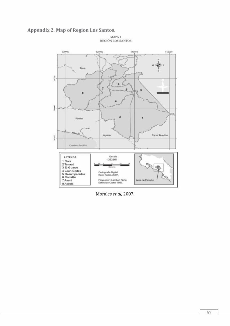
67

Appendix 2. Map of Region Los Santos.

Morales et al, 2007.

Appendix 3. Relevant Limitations and Solution This section ought to introduce a sense of criticality and nuance to our analysis. We will discuss the most important limitations to our research.

Appendix 3.1 Addressing Multi-Collinearity; Factor Analysis First of all, a common phenomenon in statistics is the issue of multi collinearity. Multi-collinearity exists when there is a strong correlation between two or more predictor variables in a regression. It can considerably bias the analysis. An effective way to deal with multi-collinearity is the application of factor analysis; this analysis is a mean of dimension reduction. It is able to identify clusters of large correlation coefficients between a subset of different variables that might be measuring the same underlying aspects (Hair et al. 2010). Factor analysis groups these variables into a single variable (factor) that shows significantly less correlation or is not associated with multi-collinearity. First thing to consider is what variables one should include. A correlation matrix between these variables can clarify this issue. Variables that frequently have correlation coefficients less than 0.3 should not be included. Table 17 at the end of this section provides the rather elaborate table necessary in order to acquire on overview on which variables to include. After reviewing this table, we omitted the variable on ‘Input Costs for Organic Fertilizer’, ‘Income Enterprise’, ‘Income Salary’ and ‘Average Educational Level’. All the other variables frequently show a correlation coefficient above 0.3. Table 15. Principal Component Analysis The table to right summarizes the results on the factor analysis. The factor analysis was conducted using principal component analysis using orthogonal rotation (varimax). The KMO measure should be higher than at least 0.5. In our case it did so we can argue that it verified the sampling adequacy for this analysis (0.875). Moreover, the Bartlett’s test has a value of 1260.41 and is significant (ρ < 0.01).

Rotated Factor Loadings

Variables Communalities 1 2

LabourCosts_Herbicide 0.773 .854 LabourCosts_Fertilization 0.686 .824 LabourCosts_Weeding 0.754 .817 Expenditures New Coffee Trees

0.684 .786

InputCosts Herbicides 0.777 .773 LabourCosts_Desucker 0.910 .677 LabourCosts_Pruning 0.635 .673 .426 InputCosts_ChemFertilizer 0.616 .616 .595 LabourCosts_PlagueContr 0.733 - .924 InputCosts_Insecticides 0.729 - .849 InputCosts_Transportation 0.687 .783 InputCosts_Fungicides 0.659 .514 .651 Size_CoffeePlots 0.733 .619 .625

% Of Variance - 41.6 % 30.5% Eigenvalues - 5.41 3.96

Factor 1 - 1.000 0.000 Factor 2 - 0.000 1.000

Note: KMO = 0.875, Bartlett’s = 1260.41 (ρ < 0.01). Non-redundant residuals = 47%.

This information mainly relates to the quality of the factors which is sufficient. In addition, the goodness of fit can also be measured. The differences between the observed correlations and the correlations based on the model are referred to as residuals. In order to be sufficient, these residuals on the correlation coefficients between the variables we have used should not exceed 0.05. Fields (2009) states that there is a reason for concern if more than 50% of the residuals exceed this number. In our case we have do not seem to have a reason for concern since the proportion of residuals that exceeds 0.05 is only 47%. Only the information on the communalities is somewhat negative, they should actually not exceed 0.7. Although the communalities for most variables are above 0.7, a considerable share lies below that number but still reasonably close to 0.7.

Appendix 3.2 Addressing Multi-Collinearity; Factors & Regression Analysis Returning to the issue of multi-collinearity; the two factors that can be interpreted as new variables do not share variation with the variables we have incorporated anymore. This is shown in the bottom part of the table on the previous page, which specifies the covariance between the two factors. It indicates the relationship between factor scores; the factor scores are uncorrelated since the diagonal elements are equal to 1. To conclude, this factor analysis has been successful in resolving the issue of multi-collinearity. A remark on the factor analysis itself relates the unbeneficial communality scores for the variables. In addition, classifying and interpreting the variables that pertain to a specific factor was also difficult. They both included some variables on labour costs and inputs costs, which make this factor analysis somewhat difficult to interpret. However, due to the focus on regression analyses in the previous chapters we will incorporate these two new variables into a multiple regression analysis in order to create more predictive power. This is contrary to the case when a regression model faces high level of multi-collinearity; this leads to difficulties in obtaining unique estimates of the regression coefficients. A plausible explanation for the high level of multi-collinearity between the variables on inputs and labour costs especially is related to the role of land. The assumption is made that labour and inputs tend to vary due to the variation in land; variation in these variables is similar since it is most likely subject to the variation in land (i.e. size of coffee plots). As the size of coffee plots tend to increase the use of input and labour tends to increase as well. The table on the next page shows the multiple regression model which incorporates these new factors. This time we have included the statistics on multi-collinearity on the right hand-side of the table. The largest VIF should not exceed 10 while the average should not be substantially bigger than 1. In addition, tolerance levels below 0,2 indicate a problem with regards to multi-collinearity (Field, 2009). Reading from the table, we do not have any cause for concern.

Table 16. Regression Model with Factors

Note: R2 = 0.71. F-statistic = 61.81, ρ < 0.01. (** ρ < 0.01).

Appendix 3.3 The Level on Sustainability The second limitations we need to add refer to the method on differentiating producers with regards to sustainability. We already mentioned that our primary focus was to compare certified to a control group of non-certified producers. However, this was not possible due to the lack of certified producers. The approach we came up with was based on ‘checklist’ of sustainable practices. The points associated with each practice should likewise lead to enable producers to increase their sustainability score by applying a specific practice. If producer would apply a specific practice they would earn the points associated with that practice. To conclude; differentiating between producers was a vital part of our research and attaching a score enabled us to do so. The scores are meant to reflect the number of sustainable practices producers incorporates during coffee production. Although the approach we chose might be arbitrary, it did lead to insights on producer characteristics while using the score we computed.

Variables B - Coefficient Standard Error B

Β1 Collinearity statistics Tolerance VIF

Constant 97.76** 25.39 -

Factor 1 69.43** 5.60 0.69 0.93 1.07

Factor 2 49.31** 5.41 0.49 0.99 1.002

Level of Sustainability

-0.33 0.96 -0.02 0.89 1.13

Average Household Education

2.01 5.31 -0.02 0.93 108

Table 17. Correlation Coefficients for Factor Analysis (** = ρ < 0.01, * = ρ < 0.05).

Size Coffee Plots

Labour Fertilization

Labour Weeding

Labour Herbicide

Labour Plague Control

Labour Pruning

Labour Desucker

Input Org. Fertilizers

Input Chem. Fertilizers

Input Insecticides

Input Fungicides

Input Herbicides

Size Coffee Plots

- ,779** ,588** ,542** ,672** ,743** ,624** ,421** ,795** ,528** ,692** ,517**

Labour Fertilization

,779** - ,648** ,673** ,442** ,701** ,612** ,458** ,670** ,318** ,526** ,621**

Labour Weeding

,588** ,648** - ,629** ,362** ,514** ,598** ,024 ,547** ,125 ,598** ,561**

Labour Herbicide

,542** ,673** ,629** - ,433** ,597** ,662** ,078 ,576** ,369** ,570** ,853**

Labour Plague Control

,672** ,442** ,362** ,433** - ,519** ,524** ,235* ,639** ,813** ,722** ,438**

Labour Pruning

,743** ,701** ,514** ,597** ,519** - ,664** ,298** ,737** ,420** ,524** ,487**

Labour Desucker

,624** ,612** ,598** ,662** ,524** ,664** - ,242* ,560** ,424** ,516** ,552*

Input Org. Fertilizer

,421** ,458** ,024 ,078 ,235** ,298** ,242** - ,178 ,059 ,132

Input Chem. Fertilizer

,795** ,670** ,547** ,576** ,639** ,737** ,560** ,178 - ,722** ,620**

Input Insecticides

,528** ,318** ,125 ,369** ,813** ,420** ,424** ,222* ,461** - ,457** ,286**

Input Fungicides

,692** ,526** ,598** ,570** ,722** ,524** ,516** ,059 ,722** 457** - ,565**

Input Herbicides

,517** ,621** ,561** ,853** ,438** ,487** ,552** ,132 ,620** ,286** ,565** -

Input Transportation

,676** ,476* ,425** ,454** ,777** ,457** ,551** ,220* ,665** ,541** ,720** ,550**

Expenditures New Trees

,621** ,714** ,632** ,756** ,442** ,592** ,569** ,250* ,565** ,444** ,531** ,602**

Income Enterprise

,352** ,126 ,023 ,111 ,553** ,159 ,236* ,157 ,313** ,608** ,380** ,085

Income Salary -,07 -,03 -,023 ,029 -,038 -,088 -,048 -,087 -,050 -,033 -,049 -,003

Average Education

,04 ,077 ,243* ,092 ,027 ,119 ,114 -,111 -,193* ,022 ,092 ,089

72

Table 17. Correlation Coefficients Factor Analysis, Continued (** = ρ < 0,01, * = ρ< 0,05)

Transportation Expenditures New Trees

Income Enterprise

Income Salary

Average Education

Size Coffee Plots

,676** ,621** ,352** -,073 ,043

Labour Fertilization

,476** ,714** ,126 -,025 ,077

Labour Weeding

,425** ,632** ,023 -,023 ,243**

Labour Herbicide

,454** ,756** ,111 ,029 ,092

Labour Plague Control

,777** ,442** ,553** -,038 ,027

Labour Pruning ,457** ,592** ,159 -,088 ,119

Labour Desucker

,551** ,569** ,236** -,048 ,114

Input Org. Fertilizer

,220* ,250* ,157 -,087 -,111

Input Chem. Fertilizer

,665** ,565** ,313** -,050 ,193*

Input Insecticides

,541** ,444** ,608** -,033 ,022

Input Fungicides

,720** ,531** ,380** -,049 ,092

Input Herbicides

,550** ,602** ,085 -,003 ,089

Input Transportation

- ,388** ,397** -,026 ,132

Expenditures New Trees

,388** - ,209* ,016 ,109

Income Enterprise

,397** ,209* - -,089 ,019

Income Salary -,026 ,016 -,089 - ,302**

Average Education

,132 ,109 ,019 ,302** -

73

Appendix 4. SPSS Output Files

Appendix 4.1. Multiple Regression ‘General Model’

74

Appendix 4.2. Multiple Regression Analysis Input Ratios

75

Appendix 4.3. Multiple Regression Analysis Labour Ratios

76

Appendix 4.4. Multiple Regression Dummy Variables Sustainability

77

Appendix 4.5. Partial Correlation; Loan Size controlling Land Size/Harvest.

78

Appendix 4.6. Multiple Regression on Degree of Sustainability

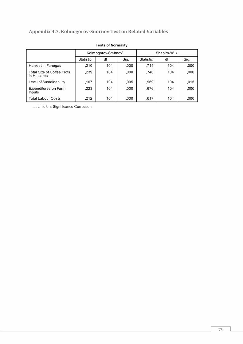
79

Appendix 4.7. Kolmogorov-Smirnov Test on Related Variables

Appendix 4.8. Kendall’s Tau Correlation Coefficients for Producer Rank on Sustainability

Appendix 4.8. Kendall’s Tau Correlation Coefficients for Producer Rank on Sustainability (Continued)

Appendix 3. Household Questionnaire

A. UBICACIÓN GEOGRÁFICA

CÓDIGO

Provincia

Distrito

Nombre

Categoría(*)

B. PERSONAL DE LA ENCUESTA CIUDAD................................................................................................1

Datos del Encuestador PUEBLO.......................................................................................2

Primer Nombre Segundo Nombre Apellido Paterno Apellido Materno Cod CASERÍO...........................................................33

ANEXO................................................................44

VILLA................................................................................................5

777

Dirección:

Masculino..........1

Femenino...........2

Relación con Jefe de Hogar (código):

Jefe de Hogar........................1 Hijo (a).....................................3 (Solo si es mayor de edad)

Cónyuge..................................2 Otro (especifique)……….....777

Años

***OBSERVACIONES (Referencias sobre la ubicación del hogar, etc):

INVESTIGACION EN EL MEDIO

AMBIENTE Y LA CADENA DE CAFE

Encuesta a hogares

Otros (Especificar)…………………………………………………………….

Centro Poblado

CÓDIGO DE

ENCUESTA

Hora de inicio:Hora de fin:

(*) Categoría de Centro Poblado:

C. NÚMERO DE AÑOS QUE EL HOGAR RESIDE EN ESTA LOCALIDAD:

Fecha de Visita

Sexo: Edad (Años cumplidos):

EXPLICACION: Este cuestionario tiene por objeto investigar la

percepción del medio ambiente y vincularlas con las prácticas

agrícolas comunes. Nos gustaría comparar entre los productores

tradicionales y sostenibles y conocer las actitudes y las motivacion

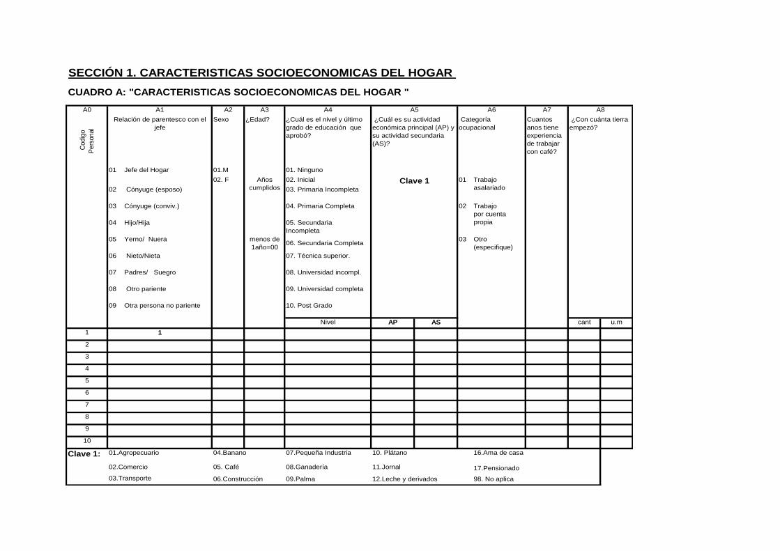
SECCIÓN 1. CARACTERISTICAS SOCIOECONOMICAS DEL HOGAR

CUADRO A: "CARACTERISTICAS SOCIOECONOMICAS DEL HOGAR "

A0 A2 A3 A7

Codig

o

Pers

onal

Sexo ¿Edad? Cuantos

anos tiene

experiencia

de trabajar

con café?

01 Jefe del Hogar 01.M

02. F 01

02 Cónyuge (esposo)

03 Cónyuge (conviv.) 02

04 Hijo/Hija

05 Yerno/ Nuera menos de

1año=00

03

06 Nieto/Nieta

07 Padres/ Suegro

08 Otro pariente

09 Otra persona no pariente

AP AS cant u.m

1

2

3

4

5

6

7

8

9

10

Clave 1: 04.Banano 07.Pequeña Industria 10. Plátano 16.Ama de casa

05. Café 08.Ganadería 11.Jornal 17.Pensionado

06.Construcción 09.Palma 12.Leche y derivados 98. No aplica

A1

1

01.Agropecuario

03.Transporte

02.Comercio

Relación de parentesco con el

jefe

A5

Clave 1 Trabajo

asalariado

A6

¿Cuál es su actividad

económica principal (AP) y

su actividad secundaria

(AS)?

Categoría

ocupacional

Años

cumplidos

07. Técnica superior.

A4

01. Ninguno

02. Inicial

¿Cuál es el nivel y último

grado de educación que

aprobó?

06. Secundaria Completa

10. Post Grado

08. Universidad incompl.

09. Universidad completa

Nivel

A8

¿Con cuánta tierra

empezó?

Otro

(especifique)

03. Primaria Incompleta

04. Primaria Completa Trabajo

por cuenta

propia05. Secundaria

Incompleta

SECCIÓN 2a. CARACTERÍSTICAS DE LA PARCELA

Nota Encuestador: Considerar todas las parcelas, tanto las en propiedad como las en uso.

CUADRO B: TENENCIA

B0 B3 B4

01

Propia y

conducida por

el hogar

01 Herencia

02 Compra

03 Adjudicación

04 Denuncio CLAVE 1

05 Invasión

06 Parcelación

07 Comunal

03 77 Otros

(especificar)

01 Plano catastrado 77 Otros

02 Escritura de la propiedad 88 No Sabe

03 Ambos 99 Ninguno

Alquilada

02

CLAVE 1

Régimen de

tenencia de la

parcela

¿Cómo adquirió

la parcela?

Código

de

Parcela

¿ En qué

año la

adquirió?

B1 B2

Sólo para parcelas propias (códigos 1

y 2 en B1)

En alquiler

¿Qué

documento

de propiedad

tiene?

86

SECCIÓN 2b. CARACTERÍSTICAS DE LA PARCELA

Nota Encuestador: Considerar todas las parcelas, tanto las en propiedad como las en uso.

CUADRO C: "CARACTERISTICAS DE LA PARCELA"

C0 C3 C4 C5 C6

01 Si Clave 1

02 No

01 Bajo 01 plana

02 Moderada 02 leve

03 Alta 03 pronunciada

99 Ninguno 88 No sabe

C2

Uso principal de la parcela

C1

CLAVE 101 Commercio Justo

La actividad

tiene

certificación

Código

de

Parcela

Superficie total

de uso

productivo

77 Otros______

Cuanto tiempo

toma para

llegar al

recibidor mas

cercano ?

¿ Cómo es la

pendiente

del terreno

en su parcela

?

Nota para el encustador: En código de parcela ubicar si se esta

hablando de dos o mas fincas separadas, con actividades diferentes

Como

percibe el

riesgo de

erosion en

su

parcela?

Extensión U.M.

01.Cultivo permanente Café

02 UTZ Certified

03 CAFE Practicas

04 Nespreso (AAA)

05 CCCC

06 Rainforest Alliance

07 Otro (especifique)

SECCIÓN 2c. CARACTERÍSTICAS DE LA PARCELA Y ACTIVOS DEL HOGAR

CUADRO D: "INVERSION EN INSTALACIONES" CUADRO E: ACTIVOS AGROPECUARIOS Y DEL HOGAR Quisiéramos ahora saber si ha

habido algún cambio en la tenencia

de activos agropecuarios en el

D0 E0 E1

Código

de

parcela

01.Vehiculo?

Camion

Pick up

Doble Tracion

Automobil

Cuadrociclo/moto

Carro

02.Bomba de Mochila

03.Tarros de leche

04. Bomba de agua

05. Motobomba

06.Otros, especificar:_________

07.Otros, especificar:_________

Casallia de VerificaciónE3.

Tiene Uds. En el hogar

Pico

Machete

Palas

Palanas

77 Otro__(especifique)

02 Drenajes

03 Naciente

D2

05 Sanitario

E2

04 Casa

¿Tienen Uds. en el hogar ..... ¿Cuántos… tiene

actualmente?

D1

01 Bodega

¿ Hace cuántos años tiene

esta instalación?

¿ Tiene en la parcela

algunas de estas

instalaciones?

¿Hace Cuantos

años lo compro?

SECCIÓN 3a. CARACTERISTICAS DEL ACUERDO

CUADRO F: CARACTERISTICAS DEL ACUERDO DE CADA COMPRADORF1 F2 F3 F4 F6 F7

¿Desde hace

quanto tiempo

le vende?

Tipo de

acuerdo

¿El comprador/

acuerdo estipula la

cantidad de cafe

entregar y cuanto?

¿El comprador /acuerdo

especifica la calidad de

cafe a entregar

(describa la calidad

entregada)?

¿El acuerdo incluye

assistencia

technica?

¿Quién es el

responsable de la

transporte de este

typo de café?

01 Ninguno 01 No 01 No 01 No 01 Productor de

Cafe

02 Acuerdo

Verbal

02 Si (especifique)

…………………

02 Si (especifique)

………………..

02 Si --> Sigue a

F6a

02 Comprador

A quien le

vende el café

03 Contrado

Firmado

F5a F5b F6a

Tipo de Cafe

Comprador

(clave 1)

¿Cuanto?

(¢ ó %)

Cuando tiemo

antes de

cosecha?

Que es la

frequencia de visita?

Clave 1

01 Microbeneficio 03 Empreza Privada

02 Cooperativa

Nota encuestador 1; Esta tabla es para cada uno de comprador al que le vende su café

Sostenible

Tradicional

Otro Typo

¿El comprador da un adelante

por cosecha?

F5

01 No

02 Si --> Sigue a F5a y F5b

SECCIÓN 3b. RELACION POR TIPOS DE COMPRADOR

CUADRO G: LAS ACTITUDES Y LA PERCEPCION SOBRE LA RELACIONMicrobeneficio Cooperativa Empreza Privada Otro Typo

01 Cierto

02 Falso

03 Indifferente

Clave 1.

Cooperacion

Flexibilidad

Dependencia y

Poder

G5. Creo que mantengo la autonomía en la mayoría de mis decisiones y la influencia externa es

limitada.

G6. En el caso que el acuerdo sea cancelado, nos enfrentaremos a problemas considerables (por

ejemplo encontrar un nuevo comprador ó una pérdida de la calidad del producto).

G3. El comprador principal es flexible en una solicitud de cambios de los acuerdo establecidos.

Nota Encuastador 1: Todos los opiniones/declaraciones son por los tipos de

compradores (si hacen negocios con este typo) que compran un tipo de producion.

G1. El comprador le informa a UD sobre el mercado y las tendencias.

G2 El comprador le informa a UD sobre las especificaciones y normas de calidad del grano de cafe.

G4. En caso de eventos inesperados, el comprador está dispuesto a hacer un nuevo acuerdo o

hacer cambios que sean aceptables y de beneficio mutuo.

SECCIÓN 4a. PRODUCCION AGROPECUARIA (Cafe)CUADRO H: INVENTARIO DE CAFETOS Y OTROS FRUTALES

H1 H2 H3 H4 H5 H6

Codigo de

ParcelaCultivo

Modo de

producción de

café

Cuanto mide?

(manzanas)

Nº total de

plantas de

café y de

árboles

Antiquedad

promedio del

lote

¿Qué tipos de café

siembra?

¿Qué otros frutales

tiene?

(Años)

Código variedad de café: 01 Caturra 02 Catuai 03 Otra(especificar)………..

Código de Cultivo: 01 Aguacate 02 Citricus 03 Platanos 04 Otro (especifcar)…………...

CUADRO I: COSECHA DE CAFÉ, FRUTALES Y CULTIVOS SEMI-PERMANENTES EN LOS ÚLTIMOS 12 MESES (Incluir pastos)I1 Cosecha (antes de

Transformación)I2 I3 I4 I5 I6 I7 I8 I9 I10 I11 I12

Totales

Total Produc.

VendidaValor ¢/.

A quien

vendio?

(clave1)

Total Produc.

VendidaValor ¢/.

A quien

vendio?

(clave1)

Total Produc.

VendidaValor ¢/.

A quien

vendio?

(clave1)

Clave 1: Comprador INGRESO TOTAL (en Colones) Σ20

1. Microbeneficio

2.Cooperativa

3. Empreza Privada

Tradicional...1

Sostenible...2

CA

FÉ

Jala

r la

s v

ari

ed

ad

es u

na p

or

un

a

OT

RO

S

FR

UT

AL

ES

OT

RO

S

FR

UT

AL

ES

Transformación Postcosecha Venta

Codigo de

Parcela

CA

FÉ

Unidades

Cosechadas

Primera calidad

Sostenible Tradicional

Otro Typo:

Especifique……………….

SECCIÓN 5. EL MEDIO AMBIENTE

CUADRO J: PERCEPCION Y ACTITUDES SOBRE EL MEDIO AMBIENTEJ4

¿Conoces el Concepto de

Servicios Ambientales?

01 Si

Mi vida cotidiana 02 No

01 Cierto 02 Falso

03 Indifferente 04 No es Aplicable

J1 J2

Produce cuidando el ambiente por

CLAVE1.

Me preocupo por el ambiente y se

refleja en

J3c. Si el estado de mi suelo (fertilidad /

J3e. Si la producion de mi cafetal es alto

CLAVE 1.

Mis practicas de

producción

Certificacion.

Otras personas (vecinos, amigos,

familia).

Produciria cuidando el medio ambiente….

J3

J3a. Si el precio de café es bueno

J3b. Si el precio de café es malo

J3h. Si el precio de las agrocuimicas es bajo

J3d. Si el estado de mi suelo (fertilidad /

erosion) es malo.

J3f. Si la producion de mi cafetal es bajo

J3g. Si el precio de las agrocuimicas es alto

92

SECCIÓN 6a. PRACTICAS & MEDIO AMBIENTE

CUADRO K: APPLICACION DE PRACTICAS A SU FINCAK1 K2

Applicado Razon

01 Si 01 Voluntaria

02 No 02 Certificacion

Conservacion del suelo

Conservacion Agronomica

Siembra en Nevel

Barreras Vivas

Coberturas Vivas (chapias)

Coberturas Muertas (dejar hojas)

Sombra

Conservacion con Estructuras Fisicas

Canales de Guardi o Desviacion

Canales de Salida

Drenaje de Ladera

Terrazas de Banco

Terrazas Individuales

Construction de Gavetas contre erosion laminar

Mejorar el Suelo

Fertilizantes Organico

Uso poco de Fertilizantes químicos

Ecosistema

Mantener la animales y naturaleza

(conservacion de ecosistema)

Control Ambiental

Control Ecologico de Plagas y Enfermedades

Uso de Pesitcidas no Estan Prohibidas

Minimizar el uso de Pesticidas

Supervisión y Rendición de Cuentas

Económicas

Registro de los Gastos, Costos y Ingresos

Totales

CUADRO L: PRACTICAS Y LA VINCULACION CON LOS SERVICIOS AMBIENTALES

L1 L2

Categorias de prácticas de producción Que beneficios recibe Uds cuando

produce cuidando el ambiente?

Que beneficios recibe la comunidad

cuando produce cuidando el ambiente?

Conservacion del Suelo

Mejorar el Suelo

Ecosistema

Control Ambiental

Que beneficios recibe su finca?

93

SECCIÓN 7. CREDITO Y PRESTAMOS

Sí………………………………………………….1 Pase siguiente pregunta

No………………………………..2 Por qué? ( ) Muy caro, ( ) Muchos trámites, ( ) Muy riesgoso, ( ) Usa mi propio dinero ( ) No es necesario

Pase Sección 8 (sgte. Página)

Sí………………………………………………….1 REGISTRE LOS DATOS EN EL CUADRO M

No………………………………..2 Pase Sección 8 (sgte. Página)

M0 M3 M4 M5 M6 M7

No. De

orden

¿Cuál es la

tasa de

interés que

le cobra?

¿Cuál es la

unidad de

tiempo a que

se refiere la

tasa de

interés?

¿Cuál es/era

el plazo del

crédito?

¿Qué tipos

de garantía le

exigió?

¿Hubiera

querido un

crédito más

grande?

(a la misma

tasa y plazo )

% Clave 2 (meses)

1. SI

2. NO -->

pase sig

Riesgo

Clave 3

01.Colones 01.Colones

Cod. 02 Dòlares 02 Dólares

1

2

3

4

5

6

7

8

Clave 1 Clave 2 Clave 3

1. Banco estatal 1. Año 1. Tierra titulada

2. Banco privado 2. Mes 2. Vivienda

3. Cooperativa o Asociación de productores 77. Otro, especifique _________________ 3. Quincena 3. La cosecha

4. ONG 4. Semana 4. Ganado

5. Prestamista 5. Día 5.Vehículo/maquinaria

6.Otro agricultor de la zona 6. Aval de otro

7.Familiar o amigo

88.No sabe

D.1 Durante los últimos 3 años, Ud. u otro miembro del hogar solicitó un crédito para la actividad de cafe

D.2 Y durante los últimos 3 años, Ud. u otro miembro del hogar recibió un crédito para la actividad de cafe

CUADRO M: CRÉDITOS RECIBIDOS DURANTE LOS ÚLTIMOS 3 AÑOS (2008-2010)

Tasa de interés:

M1 M2

Fuente del crédito Monto total del

crédito

99.Ninguno

77.Otro (especificar)

M8

Valor

¿Cuánto crédito

adicional hubiera

querido?

Clave 1

Nombre Institución

77.Otro (especificar)

8.Casa comercializadora de insumos agropecuarios y/o equipo

agropecuario

Valor

SECCIÓN 8. Percepción del Riesgo

CUADRO N: ADVERSION DE RIESGO

Está ud de acuerdo, en desacuerdo o es indiferente ante las siguientes afirmaciones:

1.Cierto

2. Falso

3. Indiferente

N.4 Invertir en nuevos cultivos es mucho riesgo, prefiero no hacerlo

N.1 Con tal de ganar dinero, estoy dispuesto a arriesgar y perder

N.2 Solamente invierto cuando estoy seguro de voy a tener una buena ganancia

N.3 Invertir en nuevos variedades de cafe es mucho riesgo, prefiero no hacerlo.

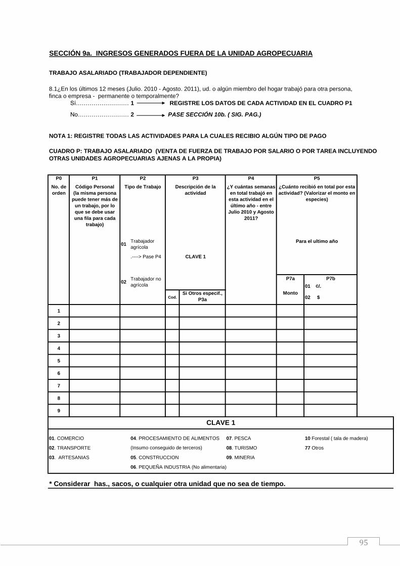
95

SECCIÓN 9a. INGRESOS GENERADOS FUERA DE LA UNIDAD AGROPECUARIA

TRABAJO ASALARIADO (TRABAJADOR DEPENDIENTE)

8.1¿En los últimos 12 meses (Julio. 2010 - Agosto. 2011), ud. o algún miembro del hogar trabajó para otra persona,

finca o empresa - permanente o temporalmente?

Sí………………………………………………….1 REGISTRE LOS DATOS DE CADA ACTIVIDAD EN EL CUADRO P1

No………………………………..2 PASE SECCIÓN 10b. ( SIG. PAG.)

NOTA 1: REGISTRE TODAS LAS ACTIVIDADES PARA LA CUALES RECIBIO ALGÚN TIPO DE PAGO

P0 P1 P4

No. de

orden

01Trabajador

agrícola

.----> Pase P4

P7a P7b

01 ¢/.

Cod.Si Otros especif.,

P3a 02 $

1

2

3

4

5

6

7

8

9

04. PROCESAMIENTO DE ALIMENTOS 07. PESCA 10 Forestal ( tala de madera)

(Insumo conseguido de terceros) 08. TURISMO 77 Otros

05. CONSTRUCCION 09. MINERIA

06. PEQUEÑA INDUSTRIA (No alimentaria)

* Considerar has., sacos, o cualquier otra unidad que no sea de tiempo.

CUADRO P: TRABAJO ASALARIADO (VENTA DE FUERZA DE TRABAJO POR SALARIO O POR TAREA INCLUYENDO

OTRAS UNIDADES AGROPECUARIAS AJENAS A LA PROPIA)

CLAVE 1

02Trabajador no

agrícola

Monto

Código Personal

(la misma persona

puede tener más de

un trabajo, por lo

que se debe usar

una fila para cada

trabajo)

¿Y cuántas semanas

en total trabajó en

esta actividad en el

último año - entre

Julio 2010 y Agosto

2011?

P2

Tipo de Trabajo

03. ARTESANIAS

02. TRANSPORTE

01. COMERCIO

CLAVE 1

P3

Descripción de la

actividad

¿Cuánto recibió en total por esta

actividad? (Valorizar el monto en

especies)

Para el ultimo año

P5

96

SECCIÓN 9b. INGRESOS GENERADOS FUERA DE LA UNIDAD AGROPECUARIA

TRABAJO NO AGROPECUARIO POR CUENTA PROPIA (TRABAJADOR INDEPENDIENTE)

Sí………………………………………………….1 REGISTRE LOS DATOS DE CADA ACTIVIDAD EN EL CUADRO Q

No………………………………..2 PASE A Secc. 11a. (Sigu. Pag.)

CUADRO Q: TRABAJO NO SALARIAL NO AGROPECUARIO

Q0 Q2 Q3 Q4

No. de

orden

¿En promedio, cuánto recibió

al mes por este

negocio/actividad ?

¿Y cuánto invirtió o gastó

por mes, en los últimos 12

meses en este

negocio/actividad ?

(Colones) (Colones)

1

2

3

4

5

6

7

8

05. CONSTRUCCION 08. TURISMO 12. PISCICULTURA

06. PEQUEÑA INDUSTRIA (No alimentaria) 09. MINERIA 13. LOMBRICULTURA

07. PESCA 10. RECOLECCION 14. FORESTAL

04. PROCESAMIENTO DE ALIMENTOS (Insumo obtenido de terceros) 11. APICULTURA 77. OTROS (ESPECIFIQUE)

03. ARTESANIAS

02. TRANSPORTE

Q1

Tipo de

negocio/actividad

CLAVE 1

Q1 77 especificarCod.

CLAVE 1

8.2 ¿En los últimos 12 meses (Julio. 2010 - Agosto 2011), ud. o algún miembro del hogar ha manejado un negocio o

trabajado por cuenta propia?

01. COMERCIO

¿Cuántos semanas

trabajó en total en este

último año en esta

actividad? (Julio 2010 a

Agosto 2011)

SECCIÓN 10a. Produccion Agropecuaria

En la actividad agrícola ¿Cuánto gastó

en:

Gasto Café

Sostenible

Gasto Café

Convencional

Monto Total

( Colones )

R11. Gastos en abonos y fertilizantes

Organicos

R22. Gastos en abonos y fertilizantes

Químicos

R3 3. Insecticidas

R4 4. Atomisos (fungicidas)

R5 5. Herbicidas

R6 6. Otros Agroquímicos

R7 7. Asesoramiento técnico

R88. Gasto en compra de sacos, canastas,

cajones, u otros envases, etc

R99. Gasto en transportes (gasolina,

lubricación, pago de flete, etc.)

Total de gastos agrícolas

CUADRO R: GASTOS EN ACTIVIDADES AGRÍCOLAS

DEL CAFÉ PARA LA PRODUCCION DE LOS ULTIMOS

12 MESES

Nota encuestador 1: En el caso de la actividad agrícola considerar los gastos para la

totalidad del último ciclo agrícola las campañas ejecutadas

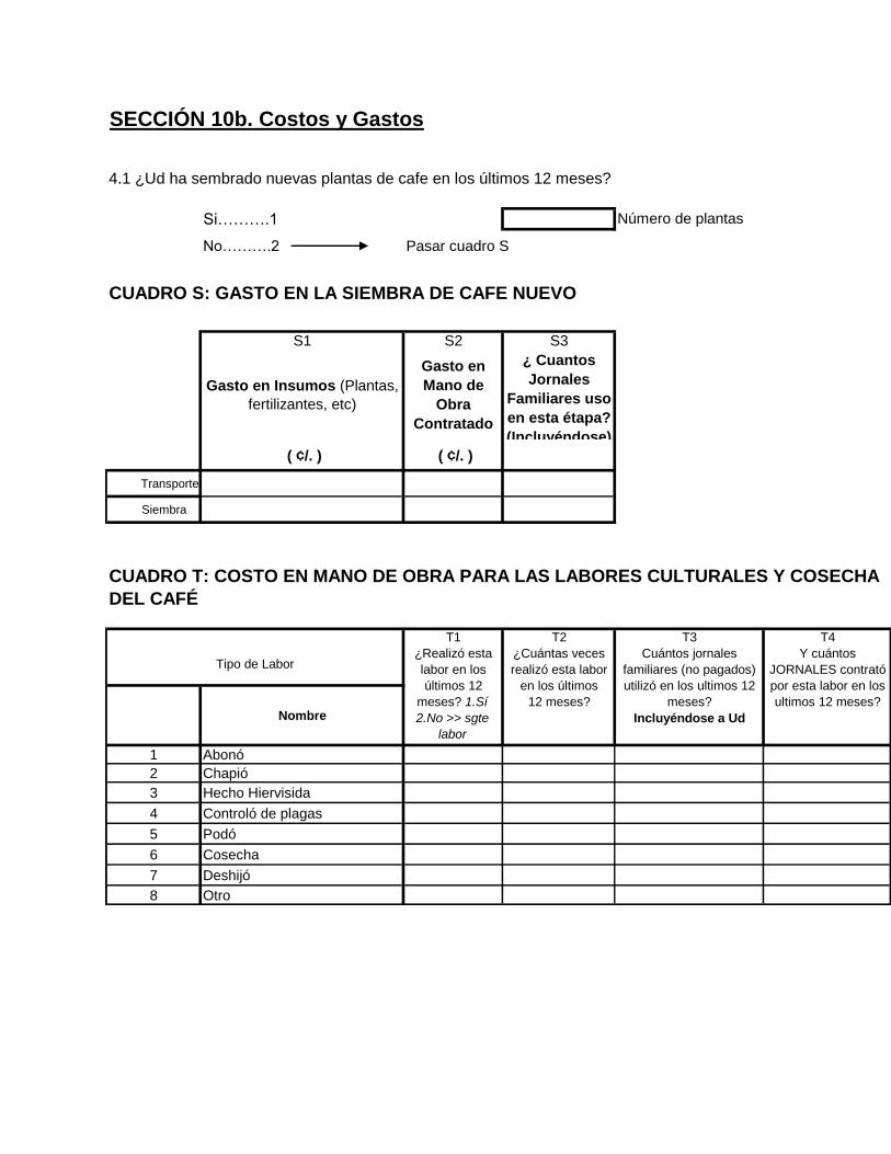
SECCIÓN 10b. Costos y Gastos

4.1 ¿Ud ha sembrado nuevas plantas de cafe en los últimos 12 meses?

Si……….1 Número de plantas

No……….2 Pasar cuadro S

CUADRO S: GASTO EN LA SIEMBRA DE CAFE NUEVO

S1 S2 S3

( ¢/. ) ( ¢/. )

Transporte

Siembra

Nombre

1 Abonó

2 Chapió

3 Hecho Hiervisida

4 Controló de plagas

5 Podó

6 Cosecha

7 Deshijó

8 Otro

T2

¿Cuántas veces

realizó esta labor

en los últimos

12 meses?

T3

Cuántos jornales

familiares (no pagados)

utilizó en los ultimos 12

meses?

Incluyéndose a Ud

T4

Y cuántos

JORNALES contrató

por esta labor en los

ultimos 12 meses?

¿ Cuantos

Jornales

Familiares uso

en esta étapa?

(Incluyéndose)

CUADRO T: COSTO EN MANO DE OBRA PARA LAS LABORES CULTURALES Y COSECHA

DEL CAFÉ

Gasto en Insumos (Plantas,

fertilizantes, etc)

Gasto en

Mano de

Obra

Contratado

Tipo de Labor

T1

¿Realizó esta

labor en los

últimos 12

meses? 1.Sí

2.No >> sgte

labor