Economics of location: A selective surveyecon2.econ.iastate.edu/faculty/kilkenny/Killk Thisse COR...

qWe thank H.A. Eiselt and a referee for useful comments and suggestions.*Corresponding author.

Computers & Operations Research 26 (1999) 1369}1394

Economics of location: A selective surveyq

Maureen Kilkenny!,*, Jacques-Franc7 ois Thisse",#

!Department of Economics, Iowa State University, IA 50011, USA"CORE, Universite& Catholique de Louvain, Belgium

#CERAS, Ecole National des Ponts et Chausse& es, France

Received 2 February 1998; received in revised form 22 June 1998

Abstract

We present a selective survey of the main results obtained in spatial economic theory. Our focus is on "rmlocation. We start with the simplest location problem and proceed to recent models of industrial location ingeneral equilibrium. The middle section is a review of what has been accomplished in the literature on spatialpricing and spatial competition. We conclude with a discussion of recent models of economic geographywhich explain the uneven spatial distribution of economic activity. ( 1999 Elsevier Science Ltd. All rightsreserved.

Keywords: Industrial location; Economic geography

1. Introduction

Economists model how scarce resources are allocated among alternatives. This paper is abouthow they model the choice among alternative geographic locations. Most of the emphasisin economics concerns location in characteristics space, where products are di!erentiated bytheir features. Geographic location choice, however, can determine the success or failure of"rms, communities, and even nations. Thus, we focus on "rm location problems in geographicspace. The selected treatments range from micro or partial equilibrium level to macro and generalequilibrium.

Micro location decisions are the kind made by "rms or people under the assumption that theirchoices do not a!ect their economic environment. For example, in a partial equilibrium model of"rm location, the opening of a new "rm is assumed to have no e!ect on local rents or wage rates. By

0305-0548/99/$ - see front matter ( 1999 Elsevier Science Ltd. All rights reserved.PII: S 0 3 0 5 - 0 5 4 8 ( 9 9 ) 0 0 0 4 1 - 6

relaxing one by one these exogeneity assumptions, economists analyze the implications of eachadditional level of complexity. Macro location models are explicit about the interdependencebetween individual location choices by people and "rms. Some models focus on the interdependen-cies between "rms; some focus on the interdependencies between industries and consumers(residential users of space), and between industries and factor markets. Classical models ofgeographic "rm location are micro models, while urban/regional models of land use patterns aremacro models.

While Regional Science, Geography, Operations Research, and other disciplines are concernedwith locational choice per se, economists are particularly concerned with the implications of thosechoices for output, prices and welfare. These correspond to economists' concerns with grossnational product, employment, in#ation, and welfare; and the public policies which a!ect thoseeconomic indicators across regions. Many economists are concerned either with national entitiesor &no place in particular'. In contrast, subsets of economists specializing in urban and regionaleconomics, local public "nance, international trade, development, and agricultural economistsconcerned with rural development are very interested in being able to explain &what happenswhere'. Urban and regional economists study spatial pricing and output, urban land use by "rmsand households, and competitive "rm location, among other topics. They explain the locations,sizes and shapes of market areas. International economists study spatial supply and demand, toexplain what will be supplied for local consumption, for export, or not at all. Developmenteconomists study the contribution to regional growth due to increasing returns to scale and cities.

Economists apply a range of mathematical techniques to location problems. The choice ofa single location may be the only variable in a "rm's decision problem. If so, it is a simplemathematical programming problem. More realistically, the choice of location is related to thechoices of product or the method of production, but it is still a micro or partial equilibrium topicamenable to analytical and mathematical programming solutions. Interdependencies among "rmsand people make some "rm location topics macro or general equilibrium problems. For interde-pendencies among "rms, game theory is employed. For interdependencies among "rms and peopleas workers and/or consumers, "xed point theorems and linear complementarity algorithms, asdeveloped by operations researchers, are often used. In this survey, we emphasize the economicproblem addressed rather than the solution technique employed.

A successful economic model rationalizes a widely observed choice pattern, or, provides insightinto how speci"ed exogenous changes a!ect choices. It must also be refutable. The basic elements ofan economic model are listed in Table 1. These include (1) the actors: who are the decision-makingagents whose choices are endogenous; (2) the objective(s): what are the goals of these agents?; (3) theendogenous variables; what instruments may the agents use to achieve their objective(s)? (4) theexogenous variables: what constrains the agents from achieving unlimited amounts of theirobjective(s)? Constraints include, for example, the parameters which de"ne the environment andthe nature of competition or market structure. The "nal aspect of an economic model is (5) what isthe relevant time horizon?

In this paper we survey models in which the objective of producers is, explicitly or implicitly, tomaximize (the expected utility of) pro"t. As suggested by Table 1, we consider a wide range ofinstruments under a variety of constraints, market structures, environments, and time horizons.The features common to economic models of location are a distance function measuring the relativeposition of places in a given space, and non-zero transport cost.

1370 M. Kilkenny, J.-F. Thisse / Computers & Operations Research 26 (1999) 1369}1394

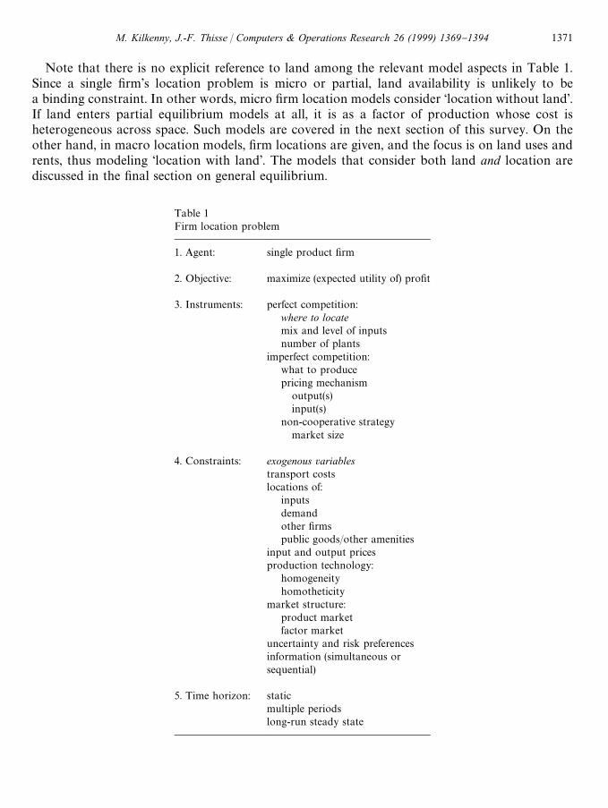
Table 1Firm location problem

1. Agent: single product "rm

2. Objective: maximize (expected utility of) pro"t

3. Instruments: perfect competition:where to locatemix and level of inputsnumber of plants

imperfect competition:what to producepricing mechanism

output(s)input(s)

non-cooperative strategymarket size

4. Constraints: exogenous variablestransport costslocations of:

inputsdemandother "rmspublic goods/other amenities

input and output pricesproduction technology:

homogeneityhomotheticity

market structure:product marketfactor market

uncertainty and risk preferencesinformation (simultaneous orsequential)

5. Time horizon: staticmultiple periodslong-run steady state

Note that there is no explicit reference to land among the relevant model aspects in Table 1.Since a single "rm's location problem is micro or partial, land availability is unlikely to bea binding constraint. In other words, micro "rm location models consider &location without land'.If land enters partial equilibrium models at all, it is as a factor of production whose cost isheterogeneous across space. Such models are covered in the next section of this survey. On theother hand, in macro location models, "rm locations are given, and the focus is on land uses andrents, thus modeling &location with land'. The models that consider both land and location arediscussed in the "nal section on general equilibrium.

M. Kilkenny, J.-F. Thisse / Computers & Operations Research 26 (1999) 1369}1394 1371

It is relevant background to recall that there are two economic theories of competition andvalue: Marshall and Arrow}Debreu [1]. Although Arrow}Debreu theory has been most popularamong non-spatial economists, Marshallian theory is more appropriate for "rm location issues.First of all, Marshallian theory is explicit about the "xed costs of production. Second, it allows forthe possibility (prevalent when space is taken into account) that "rms are large relative to demandin each market. Space puts only a few competitors in the same market area. Thus, each "rm'squantity (or pricing) decisions a!ect the price signals facing other "rms. To complement theMarshallian theory of competition and equilibrium, spatial economists use game theory to dealwith the interdependent decision-making by "rms. Noncooperative game theory models thebehavior of agents in any situation where their optimal choices depend on their forecasts of theiropponents' choices [2]. Models of location in a strategic context are considered in the third section.

Another form of interdependence among "rms in their location decisions are agglomerationeconomies. Economies of scale were described by Marshall [3] to include (i) internal scaleeconomies: declining average costs of mass production in one location, (ii) localization economies,which are external to "rms but internal to an industry, due to the formation of a specializedworkforce or expansion of specialized input provision in one location, and (iii) urbanizationeconomies which are external to industries and depend on the overall scale and scope of theeconomic activity in one location. The concentration of production activity in space is accom-panied by a concentration of population (as long as commuting to work is costly). The location ofconsumers is thus also ultimately endogenous to the location of "rms, and vice versa. There ispositive feedback between the location choices of workers/consumers and "rms. We consider thesegeneral equilibrium models last.

2. Neoclassical 5rm location

The "rst question in the neoclassical economic theory of the "rm is &what will be produced'. Theanswer is the supply curve, which expresses the level of output of a product as a function of itsmarket price, the prices of other products, prices of factors of production; and the relevanttechnological and other parameters. A powerful economic insight from location theory is that thequestions &what to produce' and &where to produce' are interchangeable, depending on consumers'preferences. Do consumers prefer homogeneous products or variety? Consider the former case:imagine a world of ubiquitous consumers who want only one type of thing. To satisfy customers, all"rms will supply the same product. If transporting the good is costly, consumers will maximizetheir utility by patronizing the "rm o!ering the lowest delivered price. Thus, "rms will maximizepro"ts by spreading out. Now consider a world where consumers prefer variety. Any number of"rms producing di!erentiated products may be able to maximize pro"t even if they all locate in thesame place. This would be reinforced if localization or urbanization scale economies also exist.Thus, spatial dispersion and/or concentration can depend on consumer preferences for concentra-tion or dispersion in characteristics space.

The second question in the neoclassical theory of the "rm is &what mix of inputs to use? Theanswer is the derived demand curve for factors of production. This question is related to the "rm'slocation decision if there is technological #exibility, or if factors prices vary across locations. In thissection, we outline the main contributions from economics on the question of "rm location. We


start with models in which location is the only choice variable in a deterministic environment, andclose with models in which location, output, and input choices are all simultaneously determinedunder uncertainty.

The basic "rm location problem is to choose one site at which pro"ts are maximized; everythingelse is given. Demand for output is parametric at constant prices everywhere. Inputs are alsoavailable at the same price across known locations. The production technology is deterministic andLeontief ("xed input coe$cients). The "rm pays the costs of transporting both inputs and outputs.The "rm is assumed to be in"nitesimally small; equivalently, markets are perfectly competitive. Thedominant paradigm in this partial equilibrium "rm location theory has been that the "rm's optimallocation is the point minimizing the weighted sum of Euclidean distances to the "nite numberof points representing markets and input sources. This is the solution to the well-knownLaunhardt}Weber problem [4].

Weber [5] approached the "rm location problem explicitly as a transport-cost minimizationproblem. He focused on multiple input sources and abstracted from any consideration of marketsales or supply areas. Isard [6] and Moses [7] showed that (given exogenous output requirements)"rms maximize pro"ts when they choose the site that minimizes transport costs if and only if inputsare used in "xed proportions.

This is an extremely partial equilibrium model insofar as the levels, mixes, and market prices forboth outputs and inputs (most variables of interest to economists) are assumed to be parametric.One location is to be chosen among the set of points on a line, in a plane, or on a topologicalnetwork. We discuss only the network representation because it resembles the real-world locationalternatives for "rms among di!erent towns (non-uniform density consumer populations) connec-ted by roads; see LabbeH et al. [8] for a comprehensive survey of location on networks.

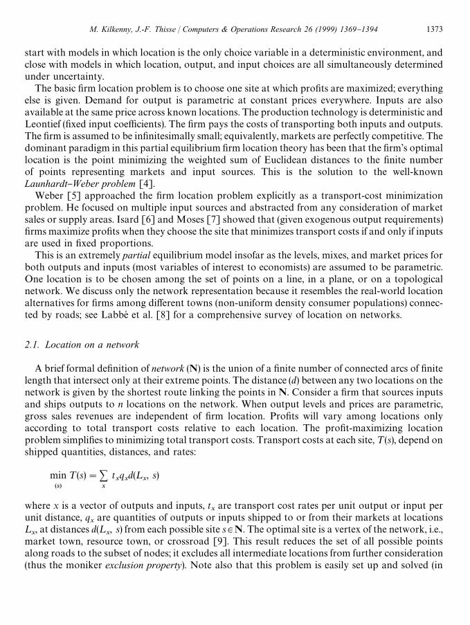
2.1. Location on a network

A brief formal de"nition of network (N) is the union of a "nite number of connected arcs of "nitelength that intersect only at their extreme points. The distance (d) between any two locations on thenetwork is given by the shortest route linking the points in N. Consider a "rm that sources inputsand ships outputs to n locations on the network. When output levels and prices are parametric,gross sales revenues are independent of "rm location. Pro"ts will vary among locations onlyaccording to total transport costs relative to each location. The pro"t-maximizing locationproblem simpli"es to minimizing total transport costs. Transport costs at each site, ¹(s), depend onshipped quantities, distances, and rates:

min(s)

¹(s)"+x

txqxd(¸

x, s)

where x is a vector of outputs and inputs, tx

are transport cost rates per unit output or input perunit distance, q

xare quantities of outputs or inputs shipped to or from their markets at locations

¸x, at distances d(¸

x, s) from each possible site s3N. The optimal site is a vertex of the network, i.e.,

market town, resource town, or crossroad [9]. This result reduces the set of all possible pointsalong roads to the subset of nodes; it excludes all intermediate locations from further consideration(thus the moniker exclusion property). Note also that this problem is easily set up and solved (in


matrix form) for the optimal location of a "rm among any predetermined and discrete number oflocation alternatives at marketplaces, resource locations, and in-between.

If transportation entails a su$ciently large "xed cost, the optimal location is a market; seeLouveaux et al. [10]. A positive discontinuity in the transport cost function at the origin isanalogous to inventory holding costs. McCann [11] models the location problem of the "rm whichalso chooses the length of time to hold inventory and the frequency of making shipments over theWeber triangle version of a network in space. Two vertices of the Weber triangle are input sourcelocations and the third is the market location. He shows that the higher the value-added, the largerthe inventory holding costs, and the stronger the motivation to economize on distance by movingcloser to the market.

Finally, if the weight of a market, de"ned as the quantities shipped to and from there times thecorresponding transport rates, exceeds the sum of the weights of the others, this market is the optimallocation of the "rm. Such a simple result may explain the locational decision made by seeminglydi!erent "rms to set up in a large metropolitan area as well as it allows us to understand the locationof steel mills next to the iron mines in the 19th century and later next to their main markets.

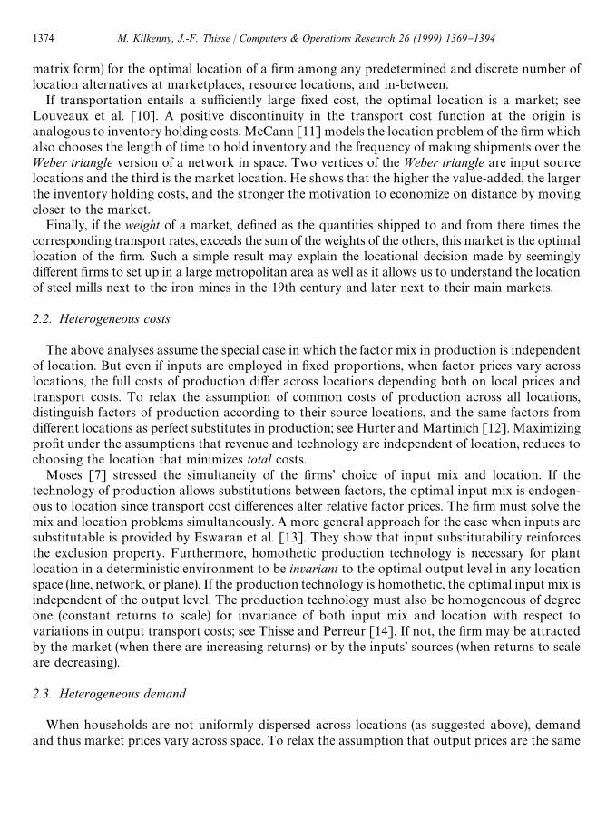
2.2. Heterogeneous costs

The above analyses assume the special case in which the factor mix in production is independentof location. But even if inputs are employed in "xed proportions, when factor prices vary acrosslocations, the full costs of production di!er across locations depending both on local prices andtransport costs. To relax the assumption of common costs of production across all locations,distinguish factors of production according to their source locations, and the same factors fromdi!erent locations as perfect substitutes in production; see Hurter and Martinich [12]. Maximizingpro"t under the assumptions that revenue and technology are independent of location, reduces tochoosing the location that minimizes total costs.

Moses [7] stressed the simultaneity of the "rms' choice of input mix and location. If thetechnology of production allows substitutions between factors, the optimal input mix is endogen-ous to location since transport cost di!erences alter relative factor prices. The "rm must solve themix and location problems simultaneously. A more general approach for the case when inputs aresubstitutable is provided by Eswaran et al. [13]. They show that input substitutability reinforcesthe exclusion property. Furthermore, homothetic production technology is necessary for plantlocation in a deterministic environment to be invariant to the optimal output level in any locationspace (line, network, or plane). If the production technology is homothetic, the optimal input mix isindependent of the output level. The production technology must also be homogeneous of degreeone (constant returns to scale) for invariance of both input mix and location with respect tovariations in output transport costs; see Thisse and Perreur [14]. If not, the "rm may be attractedby the market (when there are increasing returns) or by the inputs' sources (when returns to scaleare decreasing).

2.3. Heterogeneous demand

When households are not uniformly dispersed across locations (as suggested above), demandand thus market prices vary across space. To relax the assumption that output prices are the same


everywhere opens the possibility that total revenues also depend on location. As with spatiallyvarying input prices, we can distinguish products by their origin}destination coordinates, and treatthem as perfect substitutes in supply. The optimal site(s) are found by choosing the levels of locatedoutputs at sites(s) which maximize pro"t at the (exogenous) delivered output prices (Pm

o) less

transport costs to each of the (m) markets, and the (exogenous) factor prices (Pni) plus transport

costs from each of the (n) input locations:

max(xns

ik,xsmok )

%"

K+k/1

M+

m/1

(Pmo!t

odsm)xsm

ok!

K+k/1

N+i/1

(Pni#t

idns)xsn

ik

s. t.M+

m/1

xsmok"f (xns

ik, As) ∀k;

xsmok*0 and xns

ik*0 ∀m, i, k,

where S is the set of all possible sites, M of which are market locations (m3S; m"1,2, M), N areinput locations, (n3S, n"1,2, N), and there are K plants. F(x, As) is the production function ofoutput (indicated by subscript 0) from input x

i(from location n) and amenities As at site s3S. The

transport cost rate for output is t0, and distance between plant size s and the market at m is denoted

dsm. Likewise, transport cost rates for inputs are ti, and the distance between input source locations

n and plant site s is denoted dns. The exclusion property has been shown to hold in this context too;see Louveaux et al. [10].

2.4. Multiple plants

Due to spatial heterogeneity in resource endowments or demand, "rms may "nd it optimal toopen plants at disperse locations. If more than one site is to be considered, the key trade-o! isbetween "xed production and transport costs. LoK sch [15] and Koopmans [16] argued thatindivisibilities and/or scale economies generating "xed costs of production are essential to locationproblems. Fixed costs, however, imply that the number of plants are endogenously determined inimperfectly competitive markets. We "rst consider the multi-plant location problem with respect togiven demand at an exogenous price. There are two versions of this problem. First, a "rm mayintegrate spatially dispersed plants that are specialized, with each plant's activity chosen accordingto regional comparative advantages. Most contributions to solving the latter problem, called themulti-plant Weber problem, are rooted in Operations Research. A survey may be found inWesolowsky [4]. When inter-plant #ows are not relevant (for example, the issue is the location ofstand-alone fast-food outlets), we have the simple plant location problem. The solution to the simpleplant location problem is the number, size, and location of plants that satisfy a given demand whileminimizing "xed, variable, and transportation costs, as developed, e.g. by Manne [17], Operationsresearchers have been very active in "nding the e$cient algorithms to solve this problem; surveysare contained in Drezner [18] as well as in Mirchandani and Francis [19].

A more general version of the multi-plant location problem relaxes the assumption of perfectlyinelastic demand. In that case we may have to account for decisions concerning pricing, which willbe discussed in the next section. Hansen and Thisse [20] model the pro"t-maximizing choice ofplant numbers, sizes, locations, and pricing policy simultaneously. They con"rmed that nodes are


the optimal locations for the multi-plant "rm. They also show that when inputs are perfectsubstitutes and are supplied perfectly elastically, each input is bought by each plant from onesupply location. We must emphasize that the "rm's optimal location depends on its optimal choiceof pricing policy.

2.5. Uncertainty

The pro"tability of a site over time is not known with certainty at the time when the "xed cost ofsetting up the plant is incurred. Thus, the ex ante location decision is risky. Economists use vonNeumann}Morgenstern utility functions to represent "rms' preferences over risky alternatives.Expected pro"ts for each location strategy can be ranked by von Neumann}Morganstern utilityfunctions according to the decision-maker's degree of risk-aversion.

Hurter and Martinich [12] survey theorems regarding "rm location on linear and networkspaces with respect to output or input price, technology, and transport cost rate uncertainty. First,they consider the location problem assuming that location and input mix are determined simulta-neously, before all prices are revealed. Mathur [21] showed that the exclusion property continuesto hold if the uncertainty is in output or input prices (given transport costs that are concave indistance). Hurter and Martinich [12] explain that this follows because the variance in pro"ts due toinput or output price randomness is independent of location, assuming the input mix is determinedat the same time as the location, and the production technology is homothetic. So far, uncertaintydoes not lead to di!erent implications about location than we have already seen.

Risk matters in location choice if the location is chosen "rst, then the input mix and output level.Whether or not the exclusion property holds depends on the nature of the "rm's risk preferencesand the extent to which expected pro"ts depend on location. When uncertainty arises fromrandomness in technology, however, the variance of pro"t does depend on "rm location. It ispossible that interior locations display lower degrees of overall risk. In the same spirit, when thereare several demand points, Louveaux and Thisse [22] have shown that risk-averse "rms spreadrisks inherent in the geographical dispersion of demand by locating on an intermediate point.

The most useful way to represent technological uncertainty in an economic model of "rm locationis to formalize that the rate of output depends on #ows of input services that are random withrespect to the quantity of the inputs supplied. The randomness may re#ect variations in inputquality, supply uncertainities, or output quality variations, as well as variations in the performance(return to) of the "rm's capital. The exclusion property may not apply for risk-averse "rms if therandomness in technology varies across locations. But the solution corresponds again to thesolution in a deterministic environment, when decisions are made with respect to full prices(inclusive of risk premia). Firms substitute and/or locate away from the locus of uncertainty, andtowards the less risky locations.

The nature of risk preferences also a!ects optimal location. Consider the location problem of"rms producing one output using two inputs from di!erent locations, in a linear space. Assumethat only the price of input 1 is uncertain. The more risk averse the "rm, the less of input 1 and themore of 2 it will employ, and the closer to the input 2's source will the "rm locate. The less riskaverse "rm stays closer to input 1. In this case, di!erent locations re#ect di!erences in the degree ofrisk aversion. Also, since the full costs vary, the optimal input mix will vary from location tolocation. Even the linear homogeneity restriction that guaranteed invariance in the absence of risk


or risk aversion is insu$cient under general risk preferences and input price uncertainty. Forrisk-averse "rms, when relative input prices are uncertain, risk premia are di!erent at di!erentlevels of output. Thus, unless all "rms' risk preferences exhibit the same constant relative riskaversion, optimal input ratios can also vary at the same location because the output price plus therisk premium varies.

2.6. Summary

This section concerned partial equilibrium "rm location in a world in which perfect competitionprevails, primary factor prices are the same everywhere, but input availability and thus prices mayvary across places. The main implications are summarized by two properties: invariance andexclusion. When revenue is independent of decisions concerning costs, optimal locations (chosen tominimize total transport costs) are invariant with respect to changes (or uncertainty) in demand.The conditions for this independence include (1) market prices are exogenous (perfect competition);(2) "rms bear all transport costs; (3) the production process is homogeneous of degree 1. Ifa location problem satis"es the conditions for invariance, the cost-minimizing solution is also thepro"t-maximizing solution [13]. Regarding the second property: when (the expected utility of )pro"ts are convex over location, existing input and output market locations (nodes) are optimal(e.g., [23]) and intermediate locations are excluded. The conditions for convexity include (1)transport costs are positive and concave in distance, (2) homotheticity of the production techno-logy and (3) risk neutrality. If the problem displays these conditions, the solution to the discretelocation problem (set of nodes) is also the solution to the network one.

3. Spatial pricing and competition

Note that the "rst condition for the invariance property (above) is price exogeneity. It is rare. Themost likely reason for the endogeneity of market prices with respect to a "rm's location is thatspace gives rise to market power; see Eaton and Lipsey [24]. Perfect competition requiresnumerous alternative suppliers at comparable costs to each market location. But "rms do notlocate ubiquitously at in"nitesimally small scale. Production involves "xed costs, so industryeconomizes on the number of plants or "rms serving each market. Furthermore, transport costspenalize distant competitors, so that space gives rise to market power regardless of the totalnumber of "rms in the industry. For these reasons, a few "rms (at best) serve each local market.These few "rms are likely to be large relative to the market and thus imperfectly competitive in thesense anticipated by Marshall. The market price is not parametric, but endogenous to thequantities each "rm attempts to sell at each location. Furthermore, marginal cost pricing isincompatible with equilibrium in the presence of "xed costs. With this understanding, throughoutthis section we drop the assumption that there is an exogenous market price. Firms choose boththeir prices and their locations relative to one another.

There are (at least) two degrees of market power: monopoly and oligopoly. Note that a "rm, bydi!erentiating its product (choosing what to produce), e!ectively chooses whether to compete withother "rms or be a local monopolist. If it is a monopolist, the "rm is constrained only by the entirelocal demand (for the variety or product it supplies). The decision problem of the spatial


monopolist is to choose the spatial pricing policy and/or market area that maximizes their ownpro"ts. The extensive margin of the spatial monopolist's market size depends critically on thepricing mechanism selected. In the case of oligopoly or competitive facility location, there is at leastone competitor in the same market. Note also that market power can arise with respect to factormarkets. Monopsony can also be expected in spatial markets for inputs which are prohibitivelycostly to transport (especially land).

Greenhut et al. [25] demonstrated how critical alternative spatial pricing policies are in thelocation choice under monopoly and oligopoly. There are at least two common pricing mechan-isms: mill pricing and discriminatory pricing. Under mill pricing, the "rm o!ers the product for saleat a price p

Mto all customers. The customers travel to the "rms and bear the cost of transport.

Thus, the mill pricing mechanism is also known as the shopping mechanism. The full price toconsumers under mill pricing is p

M#ts6 . Under discriminatory pricing, the "rm incurs the transport

costs, but it charges a potentially di!erent delivered price to each consumer, chosen to maximize"rm pro"ts. The full price is p(s)"p

D(s). This latter mechanism is known as the shipping model.

Consider the distinction between shopping and shipping. Under the shopping mechanism, "rms donot observe the location of their customers. They know only the aggregate demand for theirproduct. With shipping, customers stay put while the product is delivered to them. The "rms mustknow each customer's location, and can charge a di!erent delivered price to each. In e!ect, spacesegments consumers into markets across which the monopolist can price discriminate. Theshipping model is obviously spatial price discrimination which is a particular form of third degreeprice discrimination when it charges the same (delivered) price to all consumers at the samelocation no matter how much each purchases [26].

3.1. Spatial monopoly

We begin with the single product "rm in a given location that has no competitors. The locationissue is the size of the spatial monopolist's market. Consider a one-dimensional market withcontinuously distributed consumers. The single product "rm is located at the origin (or center). Weask: (1) what pricing policy maximizes the "rm's pro"ts? (2) what will the price level be? (3) who willbear the costs of transport? (4) how large a market will the "rm serve? and "nally, (5) what are thewelfare implications of these choices? See [78] and Beckmann and Thisse [27] for a thoroughreview.

The simplest model assumes all consumers display the same linear demand behavior:

q(s)"1!p(s)

where q(s) is the quantity demanded and p(s) is the full price (price inclusive of transport costs) paidby consumers, at a distance s from the "rm. Assume also that transport costs are a simple linearfunction of distance:

t(s)"ts

and that the production technology displays constant average and marginal costs:

C(q)"cq,

where c is a positive constant.


Pro"ts (%) are prices received by the "rm net of production (and transport costs, if the "rm isresponsible for them), times demand by consumers, given consumer density *(s) over the entiremarket whose length is denoted by S:

%"PS

0

[p(s)!c!ts][1!p(s)]*(s) ds.

Clearly, the optimal monopoly price depends on the pricing mechanism, or who bears transportcosts. We focus "rst on given market with the extent of total distance S. Thus, the total marketpopulation served, M, is given by

M"PS

0

*(s) ds.

When demand is linear (1!p(s)) at each location, the total shipping distance can be expressed asthe average distance shipped times the total population served. This notation simpli"es theexpression of equilibrium price and pro"t in the shopping model. The average distance shipped, s6 ,is given by

s6":S0s*(s) ds

:S0*(s) ds

.

Consider "rst the shopping model. When customers do the shopping, pro"ts %M

are mill pricesnet of costs, times consumer demand at the average full price consumers pay:

%M"(p

M!c)M(1!p

M!ts6 ).

The "rst order condition for the shopping price, pHM, that maximizes pro"t %

Mimplies

PHM"(1#c!ts6 )/2.

Consider now the shipping model. Pro"ts under discriminatory pricing are given by

%D"P

S

0

[pD(s)!c!ts6 ][1!p

D(s)]*(s) ds.

The "rst order condition for the optimal shipping prices, pHD, are obtained by maximizing pro"t at

each location s:

pHD"(1#c#ts)/2.

Hence the pro"t-maximizing shipping monopolist absorbs half the transport costs. Accordinglycustomers have no incentives to arbitrage among themselves.

Given the market size, demand, and the respective optimal prices, we can verify that thepro"t-maximizing output is the same under both policies:

qHM"qH

D"M(1!c!ts6 )/2.

Clearly pro"ts under discriminatory pricing are higher than under mill pricing. All pro"tsdepend on the size M and the extent S of the market, as well as the density of customers.

When average costs of production are constant, any market size can be served at the same perunit production cost. Above, we assumed that the size of the market area, S, was predetermined.


Under mill or discriminatory pricing, the market extends to the distance from the "rm at whichdemand vanishes. Setting the demand function to zero and solving for SH

Mor SH

Dwe "nd

SHM"(1!pH

M)/t,

SHD"(1!c)/t.

The shipping monopolist's market is larger to the extent that the optimally chosen shoppingprice, pH

M, exceeds the marginal production cost, c, which is obviously the case. Thus the shipping

xrm will serve a larger market than the xrm patronized by shoppers. Because both market size andprice are now instruments, it can be shown that social welfare is higher under spatial pricediscrimination [28,29].

3.2. Monopolistic competition

If there are no barriers to entry to a market in which "rms are earning revenues in excess of totalcosts, other "rms will enter the industry too. Fixed costs are, however, a likely barrier to entry. Inthis section we discuss monopolistic competition, in which the size of "xed costs, relative toavailable resources or budget, limits the number of "rms in an area.

There are two models of monopolistic competition. In the "rst one, each "rm competessymmetrically with every other "rm [30]: "rms do not interact strategically because competition isnon-localized. This means that one "rms' price reduction will only marginally a!ect the demandserved by other "rms. Thus, other "rms do not react to the negligible decrease in their sales. Thearchetype of this model is by Dixit and Stiglitz [31]. This approach is used extensively in &neweconomic geography' models discussed in the next section. The second one [32] assumes thata "rm can a!ect the sales of its neighboring "rms, but not distant ones. The impact of its pricereduction is not symmetric across all locations: competition is localized. This kind of marketstructure must be studied using the tools of non-cooperative game theory. We consider bothapproaches below.

Dixit and Stiglitz [31] described monopolistic competition as a market structure determined byconsumers' preference for variety and "rms' "xed requirements for limited productive resources.Each "rm produces one variety (monopolistic), and, with freedom of entry, pro"ts will be justsu$cient to cover average costs (competition) as in Marshallian long-run equilibrium. Consumersdistinguish varieties of the &same' type of good produced by di!erent "rms, and utility is increasingin the number of varieties. Alternatively, di!erent consumers prefer and consume di!erent varieties.The varieties are demanded by each consumer to maximize intrasectoral utility represented bya constant elasticity of substitution (CES) function over the varieties from the sector:

;"C+i,s

(qsi)oD

1@o

where 0(o(1 guarantees convex preferences (convex level sets) and measures the degree ofdi!erentiation between varieties (when oP1, varieties are homogeneous). The elasticity of substi-tution, p, is related to the degree of product di!erentiation o by the relationship o"1!(1/p).When consumers choose the mix of varieties that maximize utility subject to their budgetconstraints, the "rst-order condition for pro"t maximization reveals that p is (also) the price


elasticity of demand for each variety. Hence, the demand functions are exponential, implying (asdiscussed above) that mill pricing is as pro"table as discriminatory pricing.

The simplest models assume that one variable factor of production (e.g., labor) is needed by each"rm (denoted by subscript i) to produce each unit of output for sale, Q

i, and to reproduce each unit

of "xed investment, K, which is the same for all "rms in the industry:

Qi"¸

i!K.

Note that the marginal cost of production is the local wage rate, w. Firms will price to exploit theirmonopolies over their unique varieties. Facing the constant elasticity of demand, p, "rms maximizepro"ts by equating marginal revenue to marginal cost, so that each "rms' pro"t-maximizing millprice, P

Mi, is a parametric markup over the local wage:

PMi

[1!(1/p)]"PMi

o"w

so that the equilibrium price is equal to a markup (1/o) times the local wage.Pro"ts are revenues at mill prices over costs of production:

%i"P

MiQ

i!w(Q

i#K).

Free entry drives pro"ts to zero. Thus, locations where "rm pro"ts are positive will be chosen bynew entrants. Furthermore, the implied spatial and interregional mobility of factors of productionsuggests that local wages should not be considered parametric to "rm location, and that a generalequilibrium approach is required. These extensions are discussed in the upcoming section on &neweconomic geography'.

Since PMi

equals w/o, the pro"t-maximizing level of output is a function of the elasticity ofdemand and the level of "xed costs:

Qi"oK/(1!o)"K(p!1).

The number of "rms in an area, ns, is limited by the area's supply of labor, ¸. Expressing Qiin terms

of K shows that the free entry pro"t-maximizing employment of a "rm is ¸Hi"pK, so that the

free-entry number of "rms is

ns"¸/pK

and the total number of "rms increases when products are more di!erentiated (p is smaller).When applied to spatial problems [33,34] there is an inconsistency between the local factor

supply limitation on the number of "rms and the assumption that the number of "rms is largeenough to treat each "rm as inframarginal with respect to prices and wages. The second di$culty isthe assumption that "rms establish monopoly power by di!erentiating their product(s), but thatthey do not exploit strategic opportunities with respect to other "rms. Yet, this model has provento be remarkably useful in the new economic geography models discussed below. d'Aspremontet al. [35] explain how the Dixit}Stiglitz approach can be amended to include the e!ect ofindividual pricing decisions on the price index as well as the feedback e!ect on income. Archibaldet al. [36], Lancaster [37] and Salop [38] questioned the realism of the Chamberlin/Dixit}Stiglitzassumption that the entry of a new "rm has a negligible impact on the demands facing theincumbents for spatial models. A new "rms' product necessarily crowds demand for substituteproducts. Thus, we turn to the variant which takes this into account.


The model of localized monopolistic competition focuses on the optimal size of each "rms'market assuming that "rms are mill pricers and consumers will patronize the "rm o!ering thelowest full price. The analysis determines the number and spacing of "rms that will serve a giventotal area across which consumers with limited resources are distributed. Since "rms choose pricesand locations, market areas are endogenous. The equilibrium outcome is equally spaced oligopolis-tic "rms that cover the entire market. Hence a few "rms su$ce to serve a local market. Sucha market structure requires new analytical tools.

3.3. Spatial oligopoly

The interdependence among a few "rms' location and pricing choices is best studied usingnon-cooperative game theory (see Eiselt et al. [39], for an annotated bibliography). The "rstmodern treatment of competitive "rm location is generally agreed to be Hotelling's [40] paper onduopoly in a linear market (&two ice-cream vendors on a strip of beach'). Consumers buy anundi!erentiated product from one of them. Each "rm must take the other's full price into account.We now understand Hotelling's model to be a non-cooperative game in which the players are two"rms, strategies are their locations and (mill) prices, and payo!s are "rm pro"ts. Production entailsconstant marginal costs, and transportation costs (borne by customers) are linear in distance. Thedemand side is simpli"ed dramatically: each consumer is assumed to buy only one unit of theproduct. To minimize expenditure subject to achieving the utility, consumers obviously patronizethe "rm with the lower full price.

Hotelling suggested that competition between sellers for markets would lead to concentration ofsellers in the center of the market; the Principle of minimum diwerentiation. Spatial duopolists areoften viewed as simultaneously choosing locations and prices so that neither "rm has an incentive tochange its strategy. Unfortunately, no such price-and-location equilibrium exits. Consider either ofthe following two possible location pairs. In the "rst one, "rms have di!erent locations and makedi!erent positive pro"ts; e.g., "rm 2's pro"t is higher. This induces "rm 1 to locate where "rm 2 is,and to capture the market by pricing slightly below "rm 2. If "rm 1 could increase its pro"t bychoosing the same location, di!erent locations is not an equilibrium for the duopoly. Alternatively,if both "rms choose the same location, they will compete in prices until price equals marginal cost.This is also not an equilibrium, because any unilateral deviation in price and location allows a "rmto earn positive pro"ts.

Hotelling's actual approach to the problem was to model "rms sequentially, choosing locationsthen prices. Then, the solution of the spatial duopoly problem depends critically on the nature oftransport costs and pricing policy. Consider the shopping model and assume two sellers locatealong a linear market of size l at a and b measured from the left and right endpoints of the market(a#b)l; a, b*0); and consumers are uniformly distributed along the market with a density ofone. Firm 1 understands that if it chooses a price lower than the full price customers would pay for"rm 2's product, p

1(p

2!t(l!a!b), it would capture the whole market. Alternatively, if "rm

1 prices between "rm 2's net and full price: p2!t(l!a!b))p

1)p

2#t(l!a!b), the market

boundary (at which consumers are indi!erent between "rms) will be the distance s from "rm1 where the two full prices equate

s"(p2!p

1#t(l!a!b))/2t


so that the demand facing "rm 1 is from 0 to a (left side) and s (right side). The last possibility isp1'p

2#t(l!a!b), in which "rm 2's product is cheaper to all consumers, and demand for "rm

1's product is zero.It was shown by d'Aspremont et al. [41] for a"l!b ("rms are back to back) the unique mill

price equilibrium for spatial duopolists is the competitive price: p1"p

2"c, where c denotes cost.

That "rms in a duopoly fail to raise market prices above costs to extract pro"ts is known as theBertrand Paradox [42]. For aOl!b, there is a price equilibrium under speci"c conditions onlocations [41]. In general, "rms must either both be at the center, or far apart. If "rms are neitherfar enough apart nor at the same point, mill price competition results in inde"nitely #uctuatingprices. In that case, one "rm will have an incentive to undercut the price of its rival and capture theentire market; including the rival's hinterland. The resulting discontinuity and the correspondinglack of quasiconcavity explain why an equilibrium in pure strategies does not exist when mill-pricing "rms are &too close'. If "rms are far apart, the price decrease which would allow one "rm tocapture the entire market is too much to be pro"table. These "ndings clari"ed Hotelling's claimabout the tendency of "rms to cluster at the market center while invalidating his claim that spatialdi!erentiation would yield price stability.

The inherent di$culty with the shopping version of the Hotelling duopoly problem is thediscontinuity in prices, sales, and pro"ts. One way to &smooth out' the discrete full price di!erencesis applied by d'Aspremont et al. [41]. If transport costs are quadratic rather than linear, bothdemand and pro"ts are continuous and concave in prices, and a Bertrand}Nash equilibrium existsin pure strategies. The equilibrium "rm locations are at the endpoints of the market (maximaldiwerentiation). Another approach is to relax the perfect substitutes assumption, so that the cheaperone will not always be the one purchased. de Palma et al. [43] showed that by characterizingconsumer preferences as a distribution, demand is continuous and pro"t is quasi-concave in price.In this case, as long as the distribution in preferences is disperse enough, given linear transportcosts; "rms locate at the market center and price at the same markup over cost, see also [77].

In contrast, there is no existence problem in the shipping version of the model. Under discrimina-tory pricing, "rms compete with each other for each consumer, rather than over the whole market.Since they choose a price for each consumer at each location, "rms have as many strategic variablesas there are locations. Also, "rms incur the cost of transport, so the full cost to serve consumersvaries with the locations of the consumers relative to the "rms. A "rm farther away froma particular customer can undercut its competitor's price no lower than marginal cost of produc-tion plus transport costs to that customer. The closer "rm can charge a lower price and be assuredof the sale. Thus, transport costs provide some insulation from competition for spatially price-discriminating "rms.

As a consequence, regardless of the locations of the "rms, there exists a unique equilibriumshipping price schedule over customer locations, s, which is the larger of the two full prices:

p1(s)"p

2(s)"max[c#t(s, a), c#t(s, l#b)]

as formally proven by Lederer and Hurter [44]. Note that if the "rms choose the same location(a"l!b), each customer faces a price equal to marginal plus transport costs from either shipping"rm. Note also that this price will be lower than the optimal duopoly shopping (mill) price, so thatcontrary to naive opinion, consumer welfare is higher under the discriminatory shipping regimethan shopping. Finally, the same authors show that the unique optimal locations for the two "rms


are at the "rst and third quartiles, that is, the locations minimizing total transportation costs; seealso Gabszewicz and Thisse [45].

Alternatively, the "rms' alternative to choosing prices is to choose the pro"t-maximizingquantities to sell (competition a la Cournot). It is already veri"ed that the "rms' price-locationchoice in the spatial monopoly is una!ected by which instrument (price or quantity) is chosen. Thisis not so for the shipping duopoly problem.

When transport costs are low enough such that both "rms can compete on the entire market, theequilibrium con"gurations are di!erent when the second stage is quantity rather than pricecompetition. Cournot "rms always agglomerate (locate at the center) while Bertrand "rms locate inthe "rst and third quartiles; see Hamilton et al. [46]. Thus, prices and total transport costs arelower under Bertrand competition. Finally, Cournot competition leads to node optimality (exclu-sion property); see Anderson and Neven [47] and Thisse [48].

3.4. Spatial monopsony

So far we have considered the location choices of "rms which may monopolize output markets.Now we turn to the location choices of "rms which may monopsonize input markets. A "rms'opportunity to pro"t by exploiting suppliers of a factor of production by paying a return that is lessthan the factor's marginal value depends on the elasticity of factor supply facing the "rm; see therecent literature reviewed by Boal and Ransom [49]. The more alternative employers there are, themore elastic the factor supply to any one "rm, and the less likely is monopsony power. Similarly,the more mobile the factor of production, the more elastic is factor supply, the less likely ismonopsony. Thus, immobile land is more susceptible to exploitation than mobile labor, whichexpalins why there is virtually no work on the location choice of a labor-monopsonizing "rm.There are also very few studies of land-monopsonizing "rm location, because "rm owners arerarely distinct from land owners. An exemplary exception is the colonial plantation. Models thatconsider the location of "rms which use land extensively are called plantation models.

Jones [50] presents an analysis of the optimal location, output level, input mix, factor price, andsupply area of a monopsonistic "rm that processes the raw product using a technology thatexhibits increasing returns to scale. He extends the von ThuK nen spatial land use model to "rms withmonopsony power. In general, monopsonists employ fewer inputs and produce lower output. Thismeans a monopsonist would be more market-oriented than a competitive "rm. The monopsonywould locate closer to the market, but because it uses a smaller land area, the extensive margin ofthe plantation is farther from the market than a competitive "rms'. Also, monopsony powerreduces the input's relative factor price, so the "rm uses relatively more of it and less of the otherinputs.

The spatial monopolist has been much studied. By contrast, very few papers have been writtenabout its mirror image: the spatial monopsonist. The main reason is that most results can betransferred from one to the other. LoK fgen [51] shows the analogies (as well as some minordi!erences) and argues that the spatial monopsony is worth studying because of its relevance innatural resource economics.

Yeh et al. [52] sketch the implications for a cost-minimizing monopsonist's optimal location andproduction level in a space de"ned by two input locations and one market (the &Weber triangle').They consider the location problem of a "rm that has monopsony power in only one input market,


is a price-taker in the other input and the output markets, and whose production technology ishomothetic. They argue that the optimal location is closer to the competitive input market as theoptimal output level rises. This follows because the relative price of the monopsonized input rises asoutput expands, which is o!set by a substitution away from the monopsonized input. This resultsin an increase in the locational pull of the competitively supplied input.

3.5. Central place theory

Central place theory originally described the spatial distribution of retail activity [15,53]. Itposits a hierarchy of communities in terms of numbers and diversity of retail outlets. An empiricalregularity is that the larger the population class, the fewer towns in that class, and the morenumerous and various is retail activity. The town(s) in the top population or variety category is(are) called highest order place(s). Central place theory also posits that the higher-order places o!erall of the goods o!ered at the lower order ones, but not vice versa. In its original form, central placetheory described but did not model location choice, since it identi"ed no economic force, reasonfor, or bene"t from, agglomeration [54]. The bulk of the theory has been directed towardsidentifying geometric conditions under which a superposition of regular structures is possible.However, this literature has focused far too much on geometric considerations. The models haveno economic forces which lead "rms selling di!erent goods to cluster, so it is hard to see whycentral places should emerge. In this section we discuss recent models of economically rationalagents that generate hierarchical location patterns.

Transport for certain items would be cheaper to consumers than to "rms when there are scaleeconomies unique to consumer transport. Consumers would thus have more to spend on shoppingthan shipped goods [55]. Eaton and Lipsey [54] list three forms of indivisibilities that implydecreasing average transport costs: discrete customers, discrete transport infrastructure, anddiscrete items. The "rst, in conjunction with transport activity being a disutility to consumers givesrise to multi-purpose shopping, which favors clustering. The second, for example, refers to a vehicle.The third leads to the holding of inventories, formally equivalent to a positive displacement of theorigin in each good's transport cost function equal to the inventory holding cost.

With these and a few other assumptions (including scale economies in production), Eaton andLipsey are able to generate a spatial distribution of retail "rms that does not contradict the patternshypothesized by Christaller and Losch. Di!erent goods are worth travelling di!erent distances toacquire with di!erent frequencies. Those purchased least frequently from suppliers with signi"canteconomies of scale will be o!ered only at the highest order place. Those purchased frequently fromsmall scale providers will be o!ered by "rms spacing themselves frequently to maximize salesrevenue by minimizing transport expenditures by customers.

The force driving the formation of clusters involving "rms selling di!erent goods is the occurenceof multi-purpose shopping; see Thill and Thomas [56] for a survey showing the empirical relevanceof such behavior. Consumers group their purchases of di!erent goods in order to reduce transportcosts. This creates demand externalities which "rms exploit by locating in proximity to "rms sellingother goods. Assuming nonprice competition, Eaton and Lipsey identify a set of conditions underwhich the only equilibria verify the hierarchical principle. Relaxing the assumption of anexogenous price, Thill [57] shows that a "rm selling goods of orders 1 and 2 does not locate witha "rm selling only good 1 because price competition is strong enough to push them apart. Since the


multiproduct "rm is more attractive to consumers, however, its rival locates closer than it would ifthere were only one good over which they compete.

Thus, a hierarchy may arise from economies of scope in demand. Fujita et al. [58] formalize thecentral place hierarchy by assuming that some goods are complements in demand (goods i and j arecomplements if demand for good i increases when the price of good j decreases, whenever bothgoods are consumed). They "rst show that a central location is optimal for a shopping-goodmonopolist, which establishes the highest-order central place. Next, they show that other monop-oly "rms supplying complementary will also optimally locate at the center. Ultimately they showthat multi-plant "rms will optimally open n outlets at locations to minimize transport costs.

Finally, using the Eaton}Lipsey framework, Quinzii and Thisse [59] prove that the sociallyoptimal con"guration of "rms always involves the clustering of "rms selling goods of orders 1 and2. Although these results seem to be promising, it is fair to say that the economics of central placetheory is still in infancy.

4. General equilibrium models of location

The "fth aspect of the "rm location problem outlined in Table 1 is the time horizon. Models thattake household locations as given are medium-run models at best. In the long run, people as well asxrms choose locations. Thus, in the most complex models of "rm location, household and "rmchoices are interdependent. Households compete with each other and with "rms for space, andhousehold locations determine spatial labor supply as well as spatial product demand, at full wagesand prices. Firms compete with households and each other for space, for factors of production, andfor sales. In this section we build up to the general equilibrium problem in three stages. First, wediscuss "rm location with respect to factors (i.e., labor) and the similarities with international tradetheory. Next, we overview "rm location with respect to consumer location (ignoring the labor-supply link). Finally, we outline the &new economic geography' models in which "rm, labor, andconsumer locations are interdependent in closed systems where industrial revenue equals incomeand expenditure.

4.1. Factors and technology

The "rst perspective on general spatial equilibrium (as with partial equilibrium) concerns factorendowments across locations. Di!erent types of "rms compete with each other for factors ofproduction and sales. What types of industries locate where? When a perfectly competitive marketstructure is assumed, this is the huge body of work otherwise known as the neoclassical interna-tional trade theory [60]. Taking the locations of factors as given and heterogeneous across space,the theories of comparative advantage explain why countries (locations) tend to specialize inthe production of goods that employ their relatively abundant factor(s) relatively intensively(Heckscher}Ohlin}Samuelson factor proportions models), or, in which they are relatively moreproductive (Ricardian models).

Currently, theories of comparative advantage are applied to questions raised in countries intransition from central planning to market economies as to whether or not "rms can compete inworld markets from the locations determined by the old political or &social' objectives rather than


market forces. Note that the locations of industries predicted by neoclassical trade models areequivalent to those of the neoclassical locations model with heterogeneous costs discussed earlier inthis paper. Transport costs, however, play two (minor) roles. First, they distinguish tradable fromnon-tradable goods, the latter being prohibitively expensive to transport. Second, they insulatelocal markets from distant competition (as discussed in Section 3) so that trade economists equatetransport costs with import tari!s and/or export taxes, and ignore distance per se.

Both neoclassical trade and location models explain how di!erent types of industrial "rmsoptimally match with di!erent types of locations. According to trade theory, locations aredi!erentiated by factor endowments or labor productivity. In the extreme, each location specializesin producing one thing, and trades with other locations for other products (interindustry trade).Accordingly, in location models, places are di!erentiated by their populations or material endow-ments. Each type attracts either market-oriented or materials-oriented industries. The challengehas been to explain the observed diversixcation and intraindustry trade in the context of spatialheterogeneity in factor endowments, populations, or productivity.

With respect to diversi"cation, central place theory can explain why some goods are locallysupplied in all places while other goods, produced with scale economies, are supplied only in themore populous ones, the critical trade-o! being between transport costs and "xed costs. But it doesnot explain intraindustry trade. One way to motivate intraindustry trade is through an explicitconsumer preference for variety, such as in the monopolistic competition paradigm. The monopol-istic competition model also provides a closed-form solution for long-run equilibrium underincreasing returns to scale. Krugman's [61] application of the Dixit}Stiglitz model of monopolisticcompetition formally reconciled scale economies with freedom of entry, explained intraindustrytrade, and ushered in the era of &new trade theory'. The new trade theory explains how countriesobtain comparative advantages because of scale economies, while importing and exporting thedi!erentiated goods to satisfy their tastes for variety; see Helpman and Krugman [62].

4.2. Consumer/xrm location

A broad statement of the (partial equilibrium) household problem is that residential locationsare chosen to maximize (expected) household utility over a bundle of goods, housing, leisure, andlocal public goods; given wages, employment probabilities, goods prices, commute and transportcost rates, and the locations of jobs and marketplaces. Models of urban form focus on consumers'utility over just their lot size and the quantity of the consumption good available from a centralbusiness district. The equilibrium is characterized by a spatial distribution of a given number ofconsumers that equalizes household utility at a common maximum across locations within a givenarea. Fujita [63] provides a remarkable discussion of the state of the art. The bid rent functionspeci"es the maximum rent per unit of land that a consumer can bid at any location while enjoyingthe common utility level. Land owners rent to the highest bidder. Since transport costs rise withdistance, bid rent decreases with distance.

One partial equilibrium approach to the joint "rm/consumer location problem ignores the laborsupply/"rm employment aspect as well as land use by "rms. Fujita and Thisse [64] show how anexplicit land market keeps the corresponding spatial distribution non-degenerate (not all at onepoint). They present a von Thunen}Alonso-type model of household consumption of urban land,which establishes the spatial distribution of demand facing "rms, which then compete by choosing


locations as in Hotelling. Papageorgiou and Thisse [65] and Fujita [66] model the interplay ofcentripetal/centrifugal forces with respect to interdependent consumer/"rm location. Consumerhouseholds are attracted to places with large numbers of "rms (i.e., varieties) but are repulsed bythe high rents in the desirable locations. Firms are attracted to concentrations of consumers (tominimize transport costs) but are repulsed by the competition with the other "rms also attractedthere (principle of di!erentiation). If consumers' preference for variety is strong enough, thecentripetal forces outweigh the dispersive forces, and concentration occurs. Both papers explain theformation of a downtown area around which there are relatively higher concentrations of smallretail "rms and residents.

4.3. New economic geography

Economies of scale of any type can lead to the spatial concentration of activities. Roughlyspeaking, scale economies take two forms: technological or pecuniary. Technological economiesare strictly internal to "rms. A "rm's production technology exhibits increasing returns to scale ifa doubling of inputs leads to more than a doubling of output. A "rm enjoys pecuniary economies ofscale if average revenues rise, or average costs of production decline, with volume. If average costsdecline with output because of "xed costs, the pecuniary scale economy is still internal to "rms.Average costs, however, may also decline because of the scale of an industry; for example, when anindustry becomes large enough such that a "ner division of labor is possible [67]. Scale economiesthat are external to "rms but internal to the industry within geographically delineated markets arecalled localization economies. Scale economies that are external to both the industry and "rm arecalled urbanization economies. Examples of urbanization economies include the bene"ts of labormarket pooling and extensive public infrastructure, "rst discussed by Marshall [3].

Localization economies, such as lower input prices that are available only when the size of theindustry and the level of their input demand in the locale is su$cient to support the input industryat minimum e$cient scale, are centripetal forces favoring clustering or concentration, in contrastwith the centrifugal force of competition among those same industries for customers. As discussedin the above, spatial competition leads to "rms locating far apart. In contrast, Krugman [33,34]demonstrated with his &new economic geography' models that when "rms do not competestrategically, they concentrate when transport costs are low enough.

Krugman modeled the general equilibrium problem of "rm location relative to worker/con-sumer location assuming a monopolistically competitive market structure. His formalizes twotypes of scale economies: "rms incur "xed costs (internal pecuniary scale economies) and bene"tfrom nominal wage reductions as the number of varieties available locally increases (pecuniarylocalization economies) and local population rises. Recall the monopolistic competition model byDixit and Stiglitz [31]. The elasticity of cost (percentage change in cost with respect to percentageincrease in quantity), directly expressed as the ratio of marginal (MC) to average (AC) cost, is lessthan unitary under this model:

MC/AC"w(p!1)/wp"o.

Hence the lower is p, i.e., the less substitutable varieties are in demand, the slower labor costsincrease with the scale of production; and vice versa. In sum, p is an (inverse) measure of


localization returns to scale. These ideas underline most of the analysis developed by Krugman andothers; see Fujita and Thisse [68] for a detailed survey of this literature.

The prototype model is as follows. There are two regions, two sectors, and two types of labor.A homogeneous agricultural good (A-good), ubiquitously produced (transport costs are zero)under constant returns using one type of labor (A-workers) and sold on a competitive nationalmarket. The varieties q

icorrespond to di!erentiated industrial goods (M-goods), produced by

using the other type of labor (M-workers) and sold on monopolistically competitive regionalmarkets (transport costs are positive). The A-workers are immobile whereas the M-workers areperfectly mobile. Finally, all workers/consumers have a preference for variety. In this model, theimmobility of A-workers is a centrifugal force because they consume both types of goods. Thecentripetal force is more complex. It "nds its origin in a demand ewect generated by the preference forvariety. If a larger number of producers are located in a region, the number of regional productsand consumer utility is greater. Also, because M-good "rms are mill pricers, the full equilibriumprices are lower there than in any other region. The two forces generate a real income e!ect for thecorresponding worker/consumers. This inspires workers to migrate toward the region. The result-ing increase in the local population creates a larger demand for the M-goods in the region, whichalso leads more "rms to locate there. This implies the availability of even more varieties of thedi!erentiated good, and ever higher consumer utility, in the region in question. There is circularcausation.

Krugman shows that this mechanism may give rise to a core}periphery pattern in which thewhole production of M-goods concentrates in one region. The core-periphery pattern is likely tooccur when (i) the transportation rate of the M-goods is low relative to the "xed costs ofproduction, (ii) when the M-goods are su$ciently di!erentiated, and (iii) when the share of theindustrial sector in the national economy is large enough. Minor changes in the values of thecritical parameters, furthermore, lead to dramatically di!erent equilibrium spatial con"gurations.In particular, concentrations will occur in the locations that were relatively more concentrated tobegin with. This suggests that history matters in explaining modern actual industrial locationpatterns, while the circular causation is a snowball e!ect that leads manufacturing "rms to belocked-in the same region for long time periods (examples are provided by the &industrial belt' inthe US or the so-called &blue banana' corresponding to the most industrialized areas of Europe).

Henderson [69] points out that Krugman's formalization of scale economies, however, di!ersfrom the way most urban system modelers characterize the bene"ts of localization. Urban systemsmodelers highlight the role of external economies of scale in industry}industry and indus-try}factor-market relations. Scale economies which are external to the "rm but internal to theindustry include (i) the bene"ts from the division of labor which can arise when there is enoughdownstream demand for intermediate inputs to support upstream "rms at their (larger) minimume$cient scale [67]; (ii) Marshallian labor-pooling in which workers face less unemployment riskand "rms face less adjustment cost risk in deeper labor markets; thereby lowering the transactionscosts associated with urban employment; and (iii) the bene"ts of information spillovers withinas well as between industries, and other congestable local public goods; see Rivera-Batiz andRomer [70].

A critical di!erence between urban systems and new economic geography models is that theformer are explicit about the fact that many of these forces are subject to spatial decay. Thus, thesize of the area where "rms can bene"t from localization are urbanization economies is limited. For


example, Abdel-Rahman and Fujita [71] prove the "niteness of urban areas in a model where thescale economies arise from variety in intermediate good use, so there are localization economies(even though "nal goods production is subject to constant returns to scale). A similar device isemployed by Walz [72] in his dynamic model of interdependent regions.

Another particular assumption in Krugman-style models is the perfect spatial mobility of theM-workers. While this may be reasonable for models of some countries (e.g., the US), this ceases tobe true when we come to studying the economic integration of several countries separated bycultural barriers (as in the case of the EU). Assuming that workers are spatially immobile, Venables[73] has formalized the interindustry localization form of agglomeration. He models the linkagesbetween upstream and downstream industries (as in the multifacility Weber problem) where bothindustries are assumed to be monopolistically competitive. Venables' simulations show that astransportation costs fall from high (which supports the proliferation of plants) to intermediate,"rms agglomerate to economize on the costs of shipping intermediate and "nal goods. Whicheverlocation initially has more "rms, gets more "rms; there is circular causation. However, the unevendemand for labor that follows from the geographic concentration of "rms leads to regional wagedi!erentials which cannot be sustained when transportation cost are very low. When transportcosts are very low, dispersion emerges as the equilibrium.

Helpmann [74] obtains a wider array of results about the relationship between the degree ofagglomeration and the level of transportation costs in a related model. Unlike Krugman, thedispersive forces lies in the existence of a "xed stock of land to be used for housing while individualsare all assumed to be mobile. Helpman shows that both regions accommodate industrial "rms,even though transportation costs are very low, when the demand for land is high or when productsare close substitutes. However, industrial concentration arises provided that the demand for land islow or products are di!erentiated enough, despite high transport costs. The di!erence with Krug-man lies in the fact that dispersion is here driven by region-speci"c supplies (the supply of land)instead of region-speci"c demands (the demand for manufactured goods by agricultural workers).Within Krugman's framework, this amounts to assuming arbitrarily large transport costs for theA-goods.

5. Summary

A few general principles emerge from the foregoing review. We recap in reverse: from macroto micro location decisions. First, the trade-ow between xxed production costs and transportationcosts is central to the spatial organization of an economy. This has been known since the workof LoK sch, and has been re-con"rmed recently by the numerous new economic geographycontributions triggered by Krugman. Higher "xed production costs constrain the number ofplaces where economic activities develop. Also, a reduction in transportation costs allowsfor a decline in the number of economic centers. In other words, an economy characterized by largeinvestments and low transport costs, even though endowments may be spatially homogeneous, islikely to experience uneven spatial development with many activities concentrated in only a fewplaces.

Second, product diwerentiation fosters economic agglomeration to the extent that it relaxes pricecompetition, thus allowing "rms to select close-to-market locations which minimize transport


costs. This seems to play a major role in our modern economies where di!erentiation in character-istics space substitutes for the more traditional form of geographic di!erentiation.

Third, the choice of spatial price policy also in#uences the location of "rms. Antitrust authoritiesshould be aware of that when they make (or do not make) recommendations regarding pricepolicies. Their attitude will a!ect the way "rms distribute themselves over a given territory. Firmsthat cannot charge prices to pro"tably cover transport costs do not serve as large a market as "rmsthat can. By the same token, when governments impose uniform delivered prices in attempts toimprove social welfare (or spatial equity), they actually achieve the opposite result. The moreinstruments "rms have, including pricing policy, the more e$cient they can be. Thus, social welfareis often higher when "rms are allowed to spatially price discriminate.

Fourth, transportation infrastructures have a major impact on the spatial distribution ofeconomic activities. However, this impact turns out to be very di!erent from what many regionalplanners expected. Instead of springing up anywhere along the main transportation lines, humanactivities tend to occur at the main nodes and/or the markets. The exclusion property is operative atall levels of generality: micro to macro. Thus, insights from both neoclassical location theory andnew economic geography are useful in predicting the impact of new transport technologies,characterized by low variable costs and high "xed costs, on spatial patterns in general and "rmlocation in particular. Such changes should strengthen the tendency for activity to agglomerate atexisting centers of population.

Fifth, location and production decisions are often interdependent. Similarly, the choice ofa location matters in the "rm's choice of price, and vice versa. If "rms make these decisionsindependently, they may lead to substantial losses in "rms' pro"ts. This is why facility locationanalysis would probably gain in relevance if pricing and strategic competition are integrated into theoperational models. This admittedly di$cult task could be achieved by combining, for example,operational locations models (such as those discussed in LabbeH et al. [8]) together with oligopolymodels solved by means of variational inequality techniques; see e.g., Nagurney [75] as well asLabys and Yang [76] for recent surveys.

References

[1] Novshek W, Sonnenschien H. General equilibrium with free entry. Journal of Economic Literature1987;25:1281}306.

[2] Fudenberg D, Tirole J. Game theory. Cambridge, MA: MIT Press, 1991.[3] Marshall A. Principles of economics. London: Macmillan, 1890. 8th edition published in 1920.[4] Wesolowsky G. The Weber problem: history and procedures. Location Science 1993;1:355}86.[5] Weber A. Ueber den Standort der Industrieni. TuK bingen: J.C.B. Mohr, 1909. [English translation: The Theory of

the Location of Industries. Chicago: Chicago University Press, 1929].[6] Isard W. A general location principle of an optimum space economy. Econometrica 1951;33:318}28.[7] Moses L. Location and the theory of production. Quarterly Journal of Economics 1958;72:259}72.[8] LabbeH M, Peeters D, Thisse JF. Location on networks. In: Ball MO et al., editors. Handbooks in operations

research and management science, vol. 8. Amsterdam: North-Holland, 1995:551}624.[9] Hakimi SL. Optimum location of switching centers and the absolute centers and medians of a graph. Operations

Research 1964;13:462}75.[10] Louveaux F, Thisse JF, Beguin H. Location theory and transportation costs. Regional Science and Urban

Economics 1982;12:529}45.


[11] McCann P. The logistics-cost location-production problem. Journal of Regional Science 1993;33:503}516.[12] Hurter A, Martinich JS. Facility location and the theory of production. Dordrecht: Kluwer Press, 1989.[13] Eswaran M, Kanemoto Y, Ryan D. A dual approach to the locational decision of the "rm. Journal of Regional

Science 1981;21:469}90.[14] Thisse JF, Perreur J. Relations between the point of maximum pro"t and the point of minimum transportation cost:

a restatement. Journal of Regional Science 1977;17:227}34.[15] LoK sch A. Die RaK umliche Ordnung der Wirtschaft. Jena: Gustav Fischer Verlag, 1940. [English translation: The

economics of location. New Haven, CT: Yale University Press, 1954].[16] Koopmans T. Three essays on the state of economic science. New York: McGraw-Hill, 1957.[17] Manne A. Plant location under economies of scale } Decentralization and computation. Management Science

1964;11:213}35.[18] Drezner Z, editor. Facility location: a survey of applications and methods. Heidelberg: Springer, 1995.[19] Mirchandani PB, Francis RL, editors. Discrete location theory. New York: Wiley, 1990.[20] Hansen P, Thisse JF. Multiplant location for pro"t maximisation. Environment and Planning A 1977;9:63}73.[21] Mathur VK. Location theory of the "rm under price uncertainty. Regional Science and Urban Economics

1983;13:411}28.[22] Louveaux F, Thisse JF. Production and location on a network under demand uncertainty. Operations Research

Letters 1985;4:145}9.[23] Gruver GW, Xu D. Optimal location and production: a pro"t function analysis in cartesian space. Journal of

Urban Economics 1994;35:46}70.[24] Eaton BC, Lipsey RG. The introduction of space into the neoclassical model of value theory. In: Artis M, Nobay A,

editors. Studies in modern economics. Oxford: Basil Blackwell, 1977:59}96.[25] Greenhut M, Mai Cc, Norman G. Impacts on optimum location of di!erent pricing strategies, market structure,

and consumer distributions over space. Regional Science and Urban Economics 1986;16:329}51.[26] Phlips L. The economics of price discrimination. Cambridge: Cambridge University Press, 1983.[27] Beckmann MJ, Thisse JF. The location of production activities. In: Nijkamp P, editor, Handbook of regional and

urban economics, vol. 1. Amsterdam: North-Holland, 1986:21}95.[28] Holahan WL. The welfare e!ects of spatial price discrimination. American Economic Review 1975;65(3):

498}503.[29] Hwang H, Mai Cc. E!ects of spatial price discrimination on output, welfare, and location. American Economic

Review 1990;80:567}75.[30] Chamberlin EH. The theory of monopolistic competition. Cambridge (MA): Harvard University Press, 1933.[31] Dixit AK, Stiglitz JE. Monopolistic competition and optimum product diversity. American Economic Review

1977;67:297}308.[32] Kaldor N. Market imperfection and excess capacity. Economica 1935;2:35}50.[33] Krugman P. Increasing returns and economic geography. Journal of Political Economy 1991;99:483}99.[34] Krugman P. Geography and trade. Cambridge (MA): MIT Press, 1991.[35] d'Aspremont C, Dos Santos Ferreira R, GeH rard-Varet LA. On the Dixit-Stiglitz model of monopolistic competi-

tion. American Economic Review 1996;86:623}9.[36] Archibald G, Eaton BC, Lipsey RG. Address models of value. In: Stiglitz J, Mathewson F, editors. New

Developments in the analysis of market structure. Cambridge (MA): MIT Press, 1986:3}47.[37] Lancaster K. Variety, equity, and e$ciency. New York: Columbia University Press, 1979.[38] Salop SC. Monopolistic competition with outside goods. Bell Journal of Economics 1979;10:141}56.[39] Eiselt HA, Laporte G, Thisse JF. Competitive location models: a framework and bibliography. Transportation

Science 1993;27:44}54.[40] Hotelling H. Stability in competition. Economic Journal 1929;39:41}57.[41] d'Aspremont C, Gabszewicz JJ, Thisse JF. On Hotelling's &Stability in competition'. Econometrica

1979;47:1045}50.[42] Tirole J. The theory of industrial organization. Cambridge (MA): The MIT Press, 1988.[43] de Palma A, Ginsburgh V, Papageorgiou YY, Thisse JF. The principle of minimum di!erentiation holds under

su$cient heterogeneity. Econometrica 1985;53:767}81.


[44] Lederer Ph, Hurter AP. Competition of "rms: discriminatory pricing and location. Econometrica 1986;54:623}40.[45] Gabszewicz JJ, Thisse JF. Location. In: Aumann RE, Hart S, editors. Handbook of game theory, vol. 1. Amsterdam:

North-Holland, 1992:282}304.[46] Hamilton J, Thisse JF, Weskamp A. Spatial discrimination: Bertrand vs. Cournot in a model of location choice.

Regional Science and Urban Economics 1989;19:87}102.[47] Anderson S, Neven D. Cournot competition yields spatial agglomeration. International Economic Review

1991;32:793}808.[48] Thisse J-F. Oligopoly and the polarization of space. European Economic Review 1993;37(April):299}307.[49] Boal W, Ransom M. Monopsony in the labor market. Journal of Economic Literature 1997;35:86}112.[50] Jones DW. Monopsony and plant location in a Thunen land use model. Journal of Regional Science

1988;28:317}27.[51] LoK fgren KG. The spatial monopoly: a theoretical analysis. Journal of Regional Science 1986;26:707}30.[52] Yeh Cn, Mai Cc, Shieh Yn. Location and the theory of production under monopsony. Papers in Regional Science

1996;75:433}40.[53] Christaller W. Die Zentralen Orte in SuK ddeutschland. Jena: Gustav Fischer Verlag, 1933. [English translation: The

central places of Southern Germany. Englewood Cli!s, NJ: Prentice-Hall, 1966].[54] Eaton BC, Lipsey RG. An economic theory of central places. Economic Journal 1982;92:56}72.[55] Groneberg T, Meyer J. Transport ine$ciency and the choice of spatial pricing mode. Journal of Regional Science

1981;21:541}9.[56] Thill JC, Thomas I. Toward conceptualizing trip chaining: a review. Geographical Analysis 1987;19:1}17.[57] Thill JC. Spatial duopolistic competition with multipurpose and multistop shopping. Annals of Regional Science

1992;26:287}304.[58] Fujita M, Ogawa H, Thisse JF. A spatial competition approach to central place theory: some basic principles.

Journal of Regional Science 1988;28:477}94.[59] Quinzii M, Thisse JF. On the optimality of central places. Econometrica 1990;58:1101}19.[60] Dixit AK, Norman V. Theory of international trade. Cambridge: Cambridge University Press, 1980.[61] Krugman PR. Intraindustry specialization and the gains from trade. Journal of Political Economy

1981;89(5):959}73.[62] Helpman E, Krugman P. Market structure and foreign trade. Cambridge (MA): MIT Press, 1985.[63] Fujita M. Urban economic theory. Land use and city size. Cambridge: Cambridge University Press, 1989.[64] Fujita M, Thisse JF. Spatial competition with a land market: Hotelling and von ThuK nen uni"ed. Review of

Economic Studies 1986;53:819}41.[65] Papageorgiou YY, Thisse JF. Agglomeration as spatial interdependence between "rms and households. Journal of

Economic Theory 1985;37:19}31.[66] Fujita M. A monopolistic competition model of spatial agglomeration: a di!erentiated product approach. Regional

Science and Urban Economics 1988;18:87}124.[67] Stigler G. The division of labor is limited by the extent of the market. Journal of Political Economy 1951;59:185}93.[68] Fujita M, Thisse JF. Economics of agglomeration. Journal of Japanese and International Economies

1996;10:339}78.[69] Henderson JV. Ways to think about urban concentration: neoclassical urban systems versus the new economic

geography. International Regional Science Review 1996;19:31}6.[70] Rivera-Batiz L, Romer P. Economic integration and endogenous growth. Quarterly Journal of Economics

1991;106:531}55.[71] Abdel-Rahman H, Fujita M. Product variety, Marshallian externalities, and city sizes. Journal of Regional Science

1990;30:165}83.[72] Walz U. Long-run e!ects of regional policy in an economic union. The Annals of Regional Science 1996;30:165}83.[73] Venables AJ. Equilibrium locations of vertically linked industries. International Economic Review 1996;37:

341}59.[74] Helpman E. The size of regions. In: Pines D, Sadka E, Zilcha Y, editors. Topics in public economics. New York:

Cambridge University Press, 1998:33}54.[75] Nagurney A. Network economics: A variational inequality approach. Dordrecht: Kluwer, 1993.


[76] Labys WC, Yang CW. Spatial price equilibrium as a foundation to uni"ed spatial commodity modeling. Papers inRegional Science 1997;76:1999}1228.

[77] Anderson S, de Palma A, Thisse JF. Discrete choice theory of product di!erentiation. Cambridge, MA: MIT Press,1992.

[78] Beckmann MJ. Spatial price policies revisited. Bell Journal of Economics 1976;7:619}30.


Economics of location: A selective surveyecon2.econ.iastate.edu/faculty/kilkenny/Killk Thisse COR...

Documents

Transcript of Economics of location: A selective surveyecon2.econ.iastate.edu/faculty/kilkenny/Killk Thisse COR...