Economics 173Business Statistics

Lecture 2

Fall, 2001

Professor J. Petry

http://www.cba.uiuc.edu/jpetry/Econ_173_fa01/

2

Numerical Descriptive Measures• Measures of central location

– arithmetic mean, median, mode, (geometric mean)• Measures of variability

– range, variance, standard deviation, (coefficient of variation)• Measures of association

– covariance, coefficient of correlation

3

nx

x in

1i

– This is the most popular and useful measure of central location

Sum of the measurementsNumber of measurements

Mean =

Sample mean Population mean

Nx i

N1i

Sample size Population size

nx

x in

1i

Arithmetic mean

Measures of Central Location

Sum of the measurementsNumber of measurements

Mean =

4

6xxxxxx

6x

x 654321i6

1i

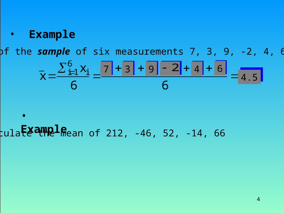
• Example

The mean of the sample of six measurements 7, 3, 9, -2, 4, 6 is given by

77 33 99 44 664.54.5

2 2

• Example

Calculate the mean of 212, -46, 52, -14, 66

5

26,26,28,29,30,32,60,31

Odd number of observations

26,26,28,29,30,32,60

Example 4.4

Seven employee salaries were recorded (in 1000s) : 28, 60, 26, 32, 30, 26, 29.Find the median salary.

– The median of a set of measurements is the value that falls in the middle when the measurements are arranged in order of magnitude.

Suppose one employee’s salary of $31,000was added to the group recorded before.Find the median salary.

Even number of observations

26,26,28,29, 30,32,60,3126,26,28,29, 30,32,60,31

There are two middle values!First, sort the salaries.Then, locate the value in the middle

First, sort the salaries.Then, locate the values in the middle26,26,28,29, 30,32,60,3129.5,

The median

6

– The mode of a set of measurements is the value that occurs most frequently.

– Set of data may have one mode (or modal class), or two or more modes.

The modal class

The mode

7

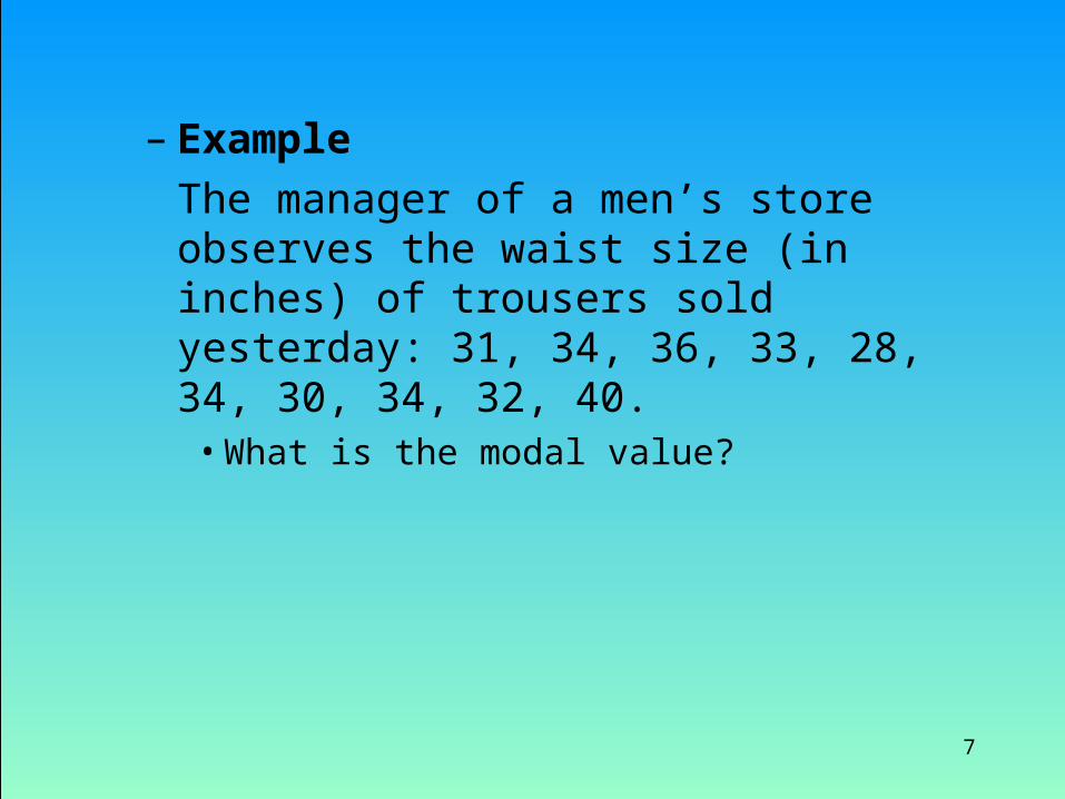
– Example

The manager of a men’s store observes the waist size (in inches) of trousers sold yesterday: 31, 34, 36, 33, 28, 34, 30, 34, 32, 40.

• What is the modal value?

8

Relationship among Mean, Median, and Mode

• If a distribution is symmetrical, the mean, median and mode coincide

• If a distribution is non symmetrical, and skewed to the left or to the right, the three measures differ.

A positively skewed distribution(“skewed to the right”)

MeanMedian

Mode

9

`

• If a distribution is symmetrical, the mean, median and mode coincide

• If a distribution is non symmetrical, and skewed to the left or to the right, the three measures differ.

A positively skewed distribution(“skewed to the right”)

MeanMedian

Mode MeanMedian

Mode

A negatively skewed distribution(“skewed to the left”)

10

Measures of variability(Looking beyond the average)

• Measures of central location fail to tell the whole story about the distribution.

• A question of interest still remains unanswered:

How typical is the average value of all the measurements in the data set?

How spread out are the measurements about the average value?

or

11

Observe two hypothetical data sets

The average value provides a good representation of thevalues in the data set.

Low variability data set

High variability data set

The same average value does not provide as good presentation of thevalues in the data set as before.

This is the previous data set. It is now changing to...

12

– The range of a set of measurements is the difference between the largest and smallest measurements.

– Its major advantage is the ease with which it can be computed.

– Its major shortcoming is its failure to provide information on the dispersion of the values between the two end points.

? ? ?

But, how do all the measurements spread out?

Smallestmeasurement

Largestmeasurement

The range cannot assist in answering this questionRange

The range

13

– This measure of dispersion reflects the values of all the measurements.

– The variance of a population of N measurements x1, x2,…,xN having a mean is defined as

– The variance of a sample of n measurementsx1, x2, …,xn having a mean is defined as

N

)x( 2i

N1i2

N

)x( 2i

N1i2

x

1n

)xx(s

2i

n1i2

1n

)xx(s

2i

n1i2

The variance

14

Consider two small populations:Population A: 8, 9, 10, 11, 12Population B: 4, 7, 10, 13, 16

1098

74 10

11 12

13 16

8-10= -2

9-10= -111-10= +1

12-10= +2

4-10 = - 6

7-10 = -3

13-10 = +3

16-10 = +6

Sum = 0

Sum = 0

The mean of both populations is 10...

…but measurements in Bare much more dispersedthen those in A.

Thus, a measure of dispersion is needed that agrees with this observation.

Let us start by calculatingthe sum of deviations

A

B

The sum of deviations is zero in both cases,therefore, another measure is needed.

15

1098

74 10

11 12

13 16

8-10= -2

9-10= -111-10= +1

12-10= +2

4-10 = - 6

7-10 = -3

13-10 = +3

16-10 = +6

Sum = 0

Sum = 0

A

B

The sum of deviations is zero in both cases,therefore, another measure is needed.

The sum of squared deviationsis used in calculating the variance.

16

Let us calculate the variance of the two populations

185

)1016()1013()1010()107()104( 222222B

25

)1012()1011()1010()109()108( 222222A

Why is the variance defined as the average squared deviation?Why not use the sum of squared deviations as a measure of dispersion instead?

After all, the sum of squared deviations increases in magnitude when the dispersionof a data set increases!!

17

Which data set has a larger dispersion?Which data set has a larger dispersion?

1 3 1 32 5

A B

Data set Bis more dispersedaround the mean

Let us calculate the sum of squared deviations for both data sets

SumA = (1-2)2 +…+(1-2)2 +(3-2)2 +… +(3-2)2= 10

SumB = (1-3)2 + (5-3)2 = 8

5 times 5 times

However, when calculated on “per observation” basis (variance), the data set dispersions are properly ranked

A2 = SumA/N = 10/5 = 2

B2 = SumB/N = 8/2 = 4!

18

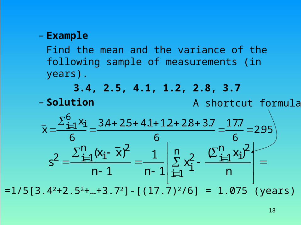
– Example

Find the mean and the variance of the following sample of measurements (in years).

3.4, 2.5, 4.1, 1.2, 2.8, 3.7– Solution

n

)x(x

1n1

1n

)xx(s

2i

n1i2

i

n

1i

2i

n1i2

95.26

7.176

7.38.22.11.45.24.36

xx i

61i

A shortcut formula

=1/5[3.42+2.52+…+3.72]-[(17.7)2/6] = 1.075 (years)

19

– The standard deviation of a set of measurements is the square root of the variance of the measurements.

– Example

Rates of return over the past 10 years for two mutual funds are shown below. Which one have a higher level of risk?

Fund A: 8.3, -6.2, 20.9, -2.7, 33.6, 42.9, 24.4, 5.2, 3.1, 30.05Fund B: 12.1, -2.8, 6.4, 12.2, 27.8, 25.3, 18.2, 10.7, -1.3, 11.4

2

2

:deviationandardstPopulation

ss:deviationstandardSample

2

2

:deviationandardstPopulation

ss:deviationstandardSample

20

– Solution– Let’s use the Excel printout that is run from the

“Descriptive statistics” sub-menu

Fund A Fund B

Mean 16 Mean 12Standard Error 5.295 Standard Error 3.152Median 14.6 Median 11.75Mode #N/A Mode #N/AStandard Deviation 16.74 Standard Deviation 9.969Sample Variance 280.3 Sample Variance 99.37Kurtosis -1.34 Kurtosis -0.46Skewness 0.217 Skewness 0.107Range 49.1 Range 30.6Minimum -6.2 Minimum -2.8Maximum 42.9 Maximum 27.8Sum 160 Sum 120Count 10 Count 10

Fund A Fund B

Mean 16 Mean 12Standard Error 5.295 Standard Error 3.152Median 14.6 Median 11.75Mode #N/A Mode #N/AStandard Deviation 16.74 Standard Deviation 9.969Sample Variance 280.3 Sample Variance 99.37Kurtosis -1.34 Kurtosis -0.46Skewness 0.217 Skewness 0.107Range 49.1 Range 30.6Minimum -6.2 Minimum -2.8Maximum 42.9 Maximum 27.8Sum 160 Sum 120Count 10 Count 10

Fund A should be consideredriskier because its standard deviation is larger

21

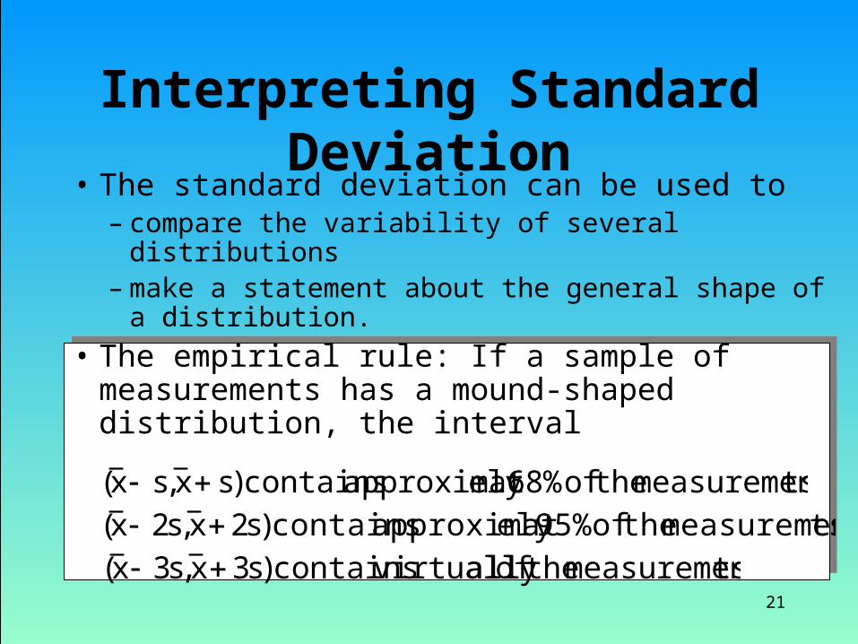
Interpreting Standard Deviation• The standard deviation can be used to

– compare the variability of several distributions– make a statement about the general shape of a

distribution. • The empirical rule: If a sample of measurements has

a mound-shaped distribution, the interval

tsmeasuremen the of 68%ely approximat contains )sx,sx( tsmeasuremen the of 95%ely approximat contains )s2x,s2x(

tsmeasuremen the of allvirtually contains )s3x,s3x(

22

– Example

The duration of 30 long-distance telephone calls are shown next. Check the empirical rule for the this set of measurements.

• Solution First check if the histogram has an approximate mound-shape

0

2

4

6

8

10

2 5 8 11 14 17 20 More

23

• Calculate the intervals:

14.55) (5.97,4.29)10.26 4.29,-(10.26 )sx,sx(

18.84) (1.68, )s2x,s2x(

23.13) (-2.61, )s3x,s3x(

• Calculate the mean and the standard deviation: Mean = 10.26; Standard deviation = 4.29.

Interval Empirical Rule Actual percentage5.97, 14.55 68% 70%1.68, 18.84 95% 96.7%-2.61, 23.13 100% 100%

Interval Empirical Rule Actual percentage5.97, 14.55 68% 70%1.68, 18.84 95% 96.7%-2.61, 23.13 100% 100%

24

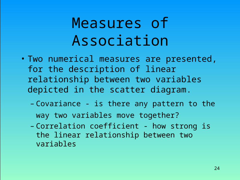
Measures of Association

• Two numerical measures are presented, for the description of linear relationship between two variables depicted in the scatter diagram.– Covariance - is there any pattern to the way two

variables move together? – Correlation coefficient - how strong is the linear

relationship between two variables

25

N

)y)((xY)COV(X,covariance Population yixi

N

)y)((xY)COV(X,covariance Population yixi

x (y) is the population mean of the variable X (Y)

N is the population size. n is the sample size.

1-n

)y)((xY)cov(X,covariance Sample yixi

1-n

)y)((xY)cov(X,covariance Sample yixi

The covariance

26

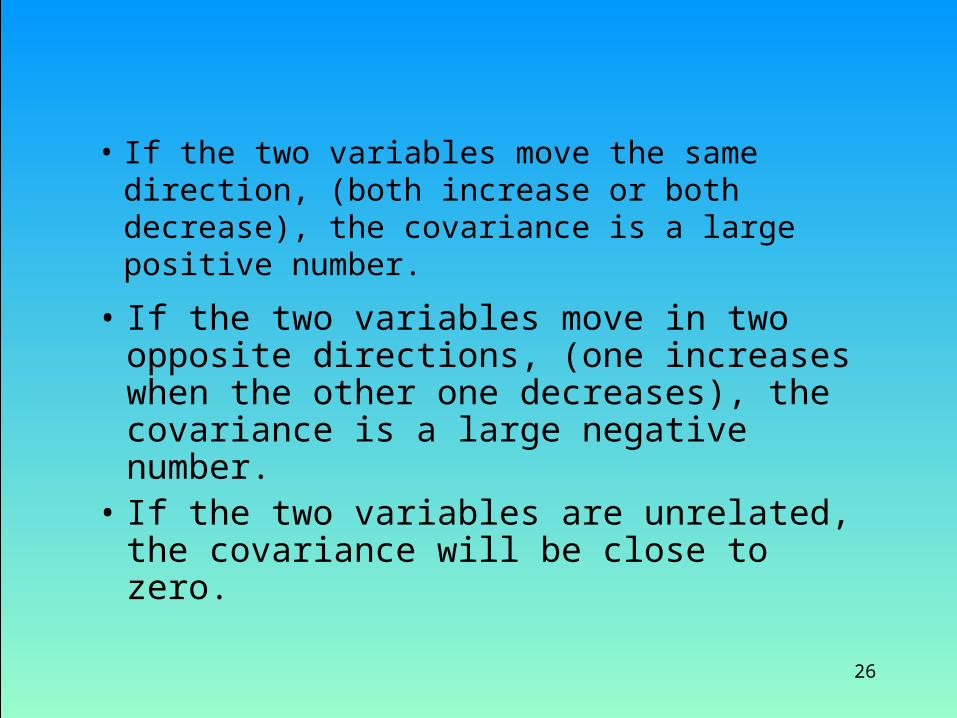
• If the two variables move in two opposite directions, (one increases when the other one decreases), the covariance is a large negative number.

• If the two variables are unrelated, the covariance will be close to zero.

• If the two variables move the same direction, (both increase or both decrease), the covariance is a large positive number.

27

– This coefficient answers the question: How strong is the association between X and Y.

yx

)Y,X(COV

ncorrelatio oft coefficien Population

yx

)Y,X(COV

ncorrelatio oft coefficien Population

yxss)Y,Xcov(

r

ncorrelatio oft coefficien Sample

yxss

)Y,Xcov(r

ncorrelatio oft coefficien Sample

The coefficient of correlation

28

COV(X,Y)=0 or r =

+1

0

-1

Strong positive linear relationship

No linear relationship

Strong negative linear relationship

or

COV(X,Y)>0

COV(X,Y)<0

29

• If the two variables are very strongly positively related, the coefficient value is close to +1 (strong positive linear relationship).

• If the two variables are very strongly negatively related, the coefficient value is close to -1 (strong negative linear relationship).

• No straight line relationship is indicated by a coefficient close to zero.

30

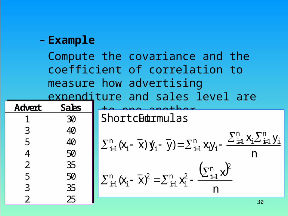
– Example

Compute the covariance and the coefficient of correlation to measure how advertising expenditure and sales level are related to one another.

n

xx)xx(

nyx

yx)yy)(xx(

FurmulasShortcut

2n1i2

in

1i2

in

1i

in

1iin

1iii

n1iii

n1i

Advert Sales1 303 405 404 502 355 503 352 25

Advert Sales1 303 405 404 502 355 503 352 25

31

• Use the procedure below to obtain the required summations

Month1 1 30 30 1 9002 3 40 120 9 16003 5 40 200 25 16004 4 50 200 16 25005 2 35 70 4 12256 5 50 250 25 25007 3 35 105 9 12258 2 25 50 4 625

Sum 25 305 1025 93 12175

x y xy x2 y2

797.839.8458.1

268.10ss

)Y,Xcov(r

yx

268.10830525

102571

nyx

yx1n

1

1n)yy)(xx(

)Y,Xcov(

in

1iin

1iii

n1i

iin

1i

458.1554.1s

554.18

2393

71

nx

x1n

1s

x

22n1i2

i2x

Similarly, sy = 8.839

32

• Excel printout

• Interpretation– The covariance (10.2679) indicates that

advertisement expenditure and sales level are positively related

– The coefficient of correlation (.797) indicates that there is a strong positive linear relationship between advertisement expenditure and sales level.

Covariance matrix Correlation matrix

Advertsmnt salesAdvertsmnt 2.125Sales 10.2679 78.125

Advertsmnt salesAdvertsmnt 2.125Sales 10.2679 78.125

AdvertsmntsalesAdvertsmnt 1Sales 0.7969 1

AdvertsmntsalesAdvertsmnt 1Sales 0.7969 1