Economic geography and wages in Brazil: Evidence...

Journal of Development Economics 91 (2010) 155–168

Contents lists available at ScienceDirect

Journal of Development Economics

j ourna l homepage: www.e lsev ie r.com/ locate /devec

Economic geography and wages in Brazil: Evidence from micro-data

Thibault Fally a, Rodrigo Paillacar b,⁎, Cristina Terra c

a PSE – Paris School of Economics, France and University of Colorado at Boulder, United Statesb CES – University of Paris 1, Paris School of Economics, Francec Université de Cergy-Pontoise: THEMA, France and EPGE –Fundação Getulio Vargas, Brazil

⁎ Corresponding author.E-mail address: [email protected] (R.

0304-3878/$ – see front matter © 2009 Elsevier B.V. Aldoi:10.1016/j.jdeveco.2009.07.005

a b s t r a c t
a r t i c l e i n f o
Article history:Received 6 May 2006Received in revised form 18 June 2009Accepted 17 July 2009

JEL classification:F12F16R12J31

Keywords:Economic geographyMarket potentialRegional disparitiesBrazilWage equation

This paper estimates the impact of market and supplier access on wage disparities across Brazilian states,incorporating the control for individual characteristics into the new economic geography methodology. Weestimate market and supplier access disaggregated by industry, and we compute access to local, national andinternational markets separately. We find a strong correlation between market access and wage differentials,even after controlling for individual characteristics, market access level (international, national or local), andusing instrumental variables.

© 2009 Elsevier B.V. All rights reserved.

1. Introduction

Brazil, the world's fifth largest country in surface area, also has oneof the highest levels of inequality. Its inequality is reflected not only atthe individual level, but also in its geographic distribution. Lall et al.(2004) report that per capita income in São Paulo, the wealthiestBrazilian state, is 7.2 times higher than in Piauí, the poorest north-eastern state. In addition, population density and market size varysubstantially across regions. Most of the population lives in the coastalareas of the north-east and south-east. While the average density inthe south-east of Brazil is over 150 inhabitants per square kilometer,this number drops below 4 for the states in the north.

New economic geography (NEG) models focus on the impact ofmarket proximity on economic outcomes, hence providing an inter-esting framework to study regional wage inequalities in Brazil. Animportant relationship put forward by NEG models is the impact oftrade costs on firm profits. Trade costs are captured by two structuralterms referred to in the literature as “market access” and “supplieraccess”. The first term measures access to potential consumers, whilethe latter refers to access to intermediate inputs. Since market andsupplier access have a positive impact on profits, the maximumwagesthat firms can afford to pay are positively related to these variables.

Paillacar).

l rights reserved.

This paper estimates a structural NEG model in order to studywage disparities across states and industries in Brazil. We use esti-mates of market and supplier access to explain regional wages, as inRedding and Venables (2004), and Head and Mayer (2006). We drawon industry-level trade data across states and control for individuals'characteristics in our estimations. Thereby, we are able to isolate theimpact of location on wage inequality from other sources of wageinequality such as differences in the composition of the labor force orthe local diversity of industries.

In two seminal works, Hanson (2005) and Redding and Venables(2004) test structural models of the new economic geography. Thefirst is applied to US counties and the second to a sampling of coun-tries. Both find a significant impact of trade costs on wages. Inspiredby this approach, intranational studies have looked at European NUTSregions (Head andMayer, 2006), US states (Knaap, 2006) and Chineseprovinces (Hering and Poncet, forthcoming).1

Our empirical framework makes two noteworthy methodologicalcontributions. First, we control for individual characteristics. Thespatial distribution of individuals could be such that their character-istics are correlated with structural NEG variables, thus leading to

1 All these papers use the methodology proposed by Redding and Venables (2004),performing a structural estimation of NEG models. Other empirical studies usealternative frameworks, such as Mion and Naticchioni (2005) for Italy, Combes et al.(2008) for France, and Lederman et al. (2004) and Da Mata et al. (2007) for Brazil.

mailto:[email protected]

http://dx.doi.org/10.1016/j.jdeveco.2009.07.005

http://www.sciencedirect.com/science/journal/03043878

156 T. Fally et al. / Journal of Development Economics 91 (2010) 155–168

spurious results in the estimation of the NEG wage equation.2 Suchcontrols are particularly important in the case of Brazil, since in-dividual diversity is vast and it is an important determinant ofwage inequalities in the country. For instance, Barros et al. (2000)show that the distribution of education and its return account forabout half of the wage inequality from observed sources in Brazil. Inaddition, we observe large differences in human capital distributionacross regions: workers from southern regions are on average moreeducated than those from northern regions. Ferreira et al. (2006) showthat over 55% of the difference in the return to labor between the north-eastern and the south-eastern regions are due to differences ineducational attainment. This substantial difference in the workforce'slevel of education across regions may be explained by sorting (Combeset al., 2008) or endogenous differences in returns to schooling (Reddingand Schott, 2003). In any case, by controlling for education we correctfor the bias induced by the differences in workforce composition acrossregions.

The secondmethodological contribution is an estimation ofmarketand supplier access using trade flows at industry level. Other studiesuse aggregate trade flows.3 This procedure alleviates the colinearityproblem found in the literature when attempts are made to estimatethese two variables simultaneously. While it is true that supply anddemand should be naturally correlated at aggregate level, sinceworkers are also consumers, it is less likely to be true at industrylevel. A firmmay rely intensively on inputs from a particular industry,while selling its product to consumers at large. Supplier access willthen be higher for regions specialized in that particular industry.Hence, by adopting this procedure we are better equipped to dis-entangle the effects of market and supplier access. As a matter offact, in the case of Brazil, the distribution of economic activity acrossregions varies a great deal across industries. Chemicals, for example,are mainly produced in Bahia, whereas transportation industries aremostly located in São Paulo.

With data on intranational and international trade flows, all dis-aggregated at industry level, we are also able to isolate local, nationaland internationalmarket and supplier access. Consequently,we are ableto establish which kinds of trade (intranational or international) havethe greatest impact on wages using a NEG mechanism.

Our empirical strategy uses a three-step procedure. Firstly, wagesare regressed on worker characteristics, controlling for state–industryfixed effects. Secondly, we estimate gravity equations by industry inorder to calculate market and supplier access for each industry ineach state. We can also compute access to international, national andlocal markets separately. Lastly, market access and supplier accessderived in the second step are used as explanatory variables for thewage disparities captured by the state–industry fixed effects in thefirst step.

We find a positive and significant effect of market and supplieraccess on the state–industry wage premium, with the impact of marketaccess being stronger than the effect of supplier access. Internationalmarket access turns out to have a greater impact than national orlocal market access. The positive impact of market access on wagesis robust after controlling for several variables, such as firm produc-tivity, taxes, regulation, endowments, and after using instrumentalvariables. The results are also unchanged in regressions at municipallevel, where we are able to further control for local amenities andendowments.

The paper is organized as follows. Section 2 describes themethodology, with a brief summary of the theoretical backgroundand a description of the empirical strategy used. The data are de-

2 To our knowledge, only Hering and Poncet (forthcoming) control for workercharacteristics in a NEG framework, and no other study has introduced firmproductivity. Mion and Naticchioni (2005) also control for individual characteristics,but in a different framework.

3 Head and Mayer (2006) also use industry-level data, but they compute marketaccess only.

scribed in Section 3, while Sections 4 and 5 discuss the results and themain robustness checks. Section 6 concludes.

2. Methodology

2.1. Theoretical framework

In economic geography models, transport costs make thegeographic distribution of demand an important determinant ofprofits. We follow in the footsteps of Head and Mayer (2006) andRedding and Venables (2004) and derive profits and market andsupplier access from Dixit–Stiglitz preferences. We present a brief de-scription of the main hypothesis and results, rather than a full-fledgedmodel, since such models are now standard in the literature.

As in the standard version of the Dixit–Stiglitz–Krugman model oftrade, we assume preferences have a constant elasticity of substitu-tion across product varieties. Each variety is produced by a single firmundermonopolistic competition. Producers and consumers are spreadover different regions, and we assume ad valorem trade costs, τrsi,between any two regions r and s.

Given these assumptions, in a symmetric equilibrium with nrifirms in region r and industry i, the value of total sales from region r toregion s, in industry i, Xrsi, can be shown to be:

Xrsiunriprixrsi =nri priτrsið Þ1−σ

P1 − σsi

Esi; ð1Þ

where xrsi represents sales of a firm in region r to region s, in industryi, pri is the price received by the firm, so that priτrsi is the price paid bya consumer in region s for a good from region r in industry i, σ is theelasticity of substitution between product varieties, and Esi is the totalregion s spending on industry i. Psi is the price index for industry i inregion s, defined as:

PsiuXr

nri priτrsið Þ1−σ

" #1=1−σ

: ð2Þ

As for production costs, we assume that firms use labor andintermediate goods as inputs, and incur a fixed cost. More precisely, inindustry i, intermediate inputs consist in a composite of goods fromall industries where ϖji is the share of expenditure on inputs fromindustry j, and, for each industry i,

Pjϖ = 1. The total price index of

intermediate inputs is equal toQjPϖji

rj .4 ‘Supplier access’ for a firm in

region r and sector i, SAri, is defined as the price index of intermediateinputs, raised to the power 1−σ, as in:

SAriuYj

P1−σrj

� �ϖji ð3Þ

It is worth noting that, in this paper, we adopt a more precisedefinition of supplier access than the NEG literature, by computingsupplier access separately for each industry, and taking into accountinter-industry linkages. This procedure helps to disentangle supplieraccess from market access. Given the definition of supplier access, totalcosts of a firm in region r and industry i may be represented bySAα = 1 − σð Þ

ri wβri fi +

Psxrsi

� �, where α and β are parameters, fi indicates

the fixed cost in industry i, andwri is the wage in region r and industry i.5

Supplier access is a measure of the firm's access to intermediate inputs,and it is negatively related to trade costs. The greater the supplier access,the lower the cost of intermediate inputs.

4 This specification of the price index of intermediate inputs may be derived from aCobb–Douglas production function, using input from all other industries.

5 We assume that labor migration across regions is not high enough to arbitrageaway all regional wage disparities.

8 In keeping with most of the labor literature, we focus on male workers betweenthe ages of 25 and 65, because the wage dynamics and labor supply of the femaleworkforce are often affected by non-economic factors, such as fertility decisions.

9 In Section 5.4, on robustness checks, this equation will be estimated adding inproductivity as the explanatory variable. In that case, the regression will incorporatethe firm dimension.

157T. Fally et al. / Journal of Development Economics 91 (2010) 155–168

In maximizing profits, prices are set as a constant mark-up overmarginal cost. Profits, then, can be shown to be given by:

Πri =1σ

SAα = 1−σð Þri wβ

ri

� �1−σMAri − fiSA

α = 1 − σð Þri wβ

ri ð4Þ

where MAri is ‘market access’, or ‘real market potential’, as referred toby Head and Mayer (2006), defined as:

MAriuXs

τ1 − σrsi EsiP1 − σsi

!ð5Þ

Market access will be greater when trade costs are lower and thereal expenditure of the importing region is larger. The greater themarket access, the higher the potential demand for the region'sproducts in industry i.

We are able to relate regional wages to market access and supplieraccess (hereafter, MA and SA, respectively). With free entry, profits arenecessarily zero in equilibrium. Given the profit function in Eq. (4), thisequilibrium condition yields:

wri =MAri

σ fi

� � 1βσ

SAα

β σ − 1ð Þri ð6Þ

Hence, wages are higher in regions with greater MA, that is, withlow trade costs to importing regions with high spending. Also, wagesare higher in regions with greater SA, that is, where inputs can bebought at low prices due to low transport costs to suppliers.

2.2. Empirical strategy

Our empirical use of the theoretical framework described aboveinvolves a three-step strategy in a cross-sectional analysis for 1999.6

Firstly, wages are regressed on worker characteristics, includingstate–industry fixed effects. The wage premium captured by thesefixed effects is the variable to be explained by market and supplieraccess. Secondly, in keeping with the new economic geography liter-ature, we estimate gravity equations in order to calculate market andsupplier access for each state and industry pair. Finally, market accessand supplier access derived in the second step are used as explanatoryvariables for wage disparities captured by state–industry fixed effectsfrom the first step.7 We explain each step in turn.

2.2.1. First stepAlthough the theoretical framework described in the previous

subsections treats labor as a homogeneous factor of production, weknow that this is not the case. There is extensive literature explainingwage differences across individuals by means of their characteristics,such as educational attainment, experience in years, gender andmarital status, among many other variables. For Brazil, in particular,Langoni's seminal work (1973) presents evidence of the importanceof worker heterogeneity in income inequality. If patterns of diversityamong individuals in the labor force were similar across regions, wecould still explain average regional wages by regional market andsupplier access differences, as proposed in Eq. (6). Previous empiricalwork, however, has identified substantial differences in the compo-sition of the labor force across Brazilian regions, especially withrespect to educational attainment (see Ferreira et al., 2006). Thus, ourresults would be biased if we did not control for individual char-

6 We limit our analysis to 1999 due to the lack of intranational trade data for otherperiods in Brazil, as explained in Section 3.

7 We thank an anonymous referee for suggesting an empirical procedure wherefixed effects from the wage equation are regressed on market and supplier access.

acteristics and sorting across regions and sectors. The first step of ourempirical study consists in estimating the following equation:

logwl;ri = λ1agel;ri + λ2age2l;ri +

X9m=1

μmedml;ri + ωri + nl;ri ð7Þ

where wl,ri is the wage of a male8 worker l working in industry i, ofregion r, agel,ri is the worker's age, edl,rim is a dummy variable for eachof the nine educational levels (see Appendix A1), and ωri are dummyvariables for each state–industry pair.9

State–industry fixed effects capture wage disparities that are notexplained by worker characteristics. In the third step of our empiricalprocedure, these fixed effects will be explained by market access andsupplier access.

2.2.2. Second stepThe second step consists in estimating MA and SA as follows. Total

sales from region r to region s in industry i, from Eq. (1), can bewritten as:

logXrsi = log nriprið Þ + 1− σð Þlogτrsi + logEsi

P1 − σsi

ð8Þ

The first term in the right-hand side of Eq. (8) comprises variablesrelated to the exporting region, while the third term involvesvariables exclusively from the importing region. Hence, these twoterms are captured empirically by exporting and importing regionfixed effects, FXri and FMsi, respectively. As for the second term, thereis no single variable to capture trade costs between two regions. Tradecosts will then be captured by a set of variables, TCk,rs, such as thedistance between the regions (in log), whether they share borders, alanguage, or whether they have a colonial link.10 In sum, Eq. (8) isestimated by means of a gravity equation as follows:

logXrsi = FXri +Xk

δkiTCk;rs + FMsi + ersi ð9Þ

where Xrsi stands for exports from region r to region s in industry i,and εrsi is an error term. A region may be defined as either a Brazilianstate or one of the 210 countries in our dataset.

In order to render our results comparable to those in the literature,we have also estimated Eq. (9) for aggregate trade flows, instead ofdisaggregating by industry. In this way, we can compute MA and SAmeasures comparable to those in Redding and Venables (2004),Knaap (2006), Head and Mayer (2006), and Hering and Poncet(forthcoming).

We would like to note that an estimation based on gravity re-gressions has the advantage of using information on the economicmechanism that our theoretical model intends to stress, namely,spatial interactions arising from trade.Wewould thus be less prone tocapture other effects of proximity, such as technological or urbanexternalities. Nevertheless, we will perform a number of robustnesschecks to investigate a potential correlation between the tradechannel and other covariates and competing explanations.

10 A number of alternative sets of variables could be chosen, but changing gravityequation specifications makes little difference to the final-step results. Similar resultsare obtained, for example, when we introduce a dummy for pairs of countriesbelonging to MERCOSUR, when we introduce distances by road (for intranational tradeonly) instead of physical distance, and when we estimate differentiated distancecoefficients for intranational versus international trade. Lastly, Paillacar (2007) showsthat Gamma PML yields similar results to OLS.

12 Because of the huge number of observations, we run our regressions on randomsamples of 500,000 or 800,000 employees (out of 2,786,852 employees in the fullsample). Changing the size of the sample does not affect our coefficients nor does it


Despite their empirical success in explaining trade flows, gravityequations have an important caveat: they treat the size of regions asexogenous (Knaap, 2006). We acknowledge this limitation in explain-ing the long-term evolution of a country's economic geography, andwe see ourwork as an effort to uncover the impact ofmarket access onwages, taking the spatial distribution of economic activity as given.

From Eq. (5), the estimated coefficients in Eq. (9) can be used tocompute market access as in:

MAriuXs

expFMsið ÞYk

expTCk;rsi

� �δki" #ð10Þ

We have, then, a market access measure for each separate industryin each Brazilian state.

The estimated value of SA, defined in Eq. (3), is computed in asimilar fashion, but using the coefficient from the exporting regiondummy variables. To account for vertical linkages across industries,we use coefficients from the input–output matrix, ϖ, to weigh theimpact of each industry in supply access. We, then, compute:

SAriuYj

Xs

expFXsj

� �Yk

expTCk;rsj

� �δkj" #( )ϖji

ð11Þ

which yields an SA measure for each industry in each Brazilian state.This paper is the first to weigh industry supplier access using an

input–output matrix in the structural approach proposed by Reddingand Venables (2004). Amiti and Cameron (2007) also take intoaccount industry vertical linkages in a study for Indonesia, but with asomewhat different empirical strategy. In their computation of SA,they use the shares of GDP by industry for each Indonesian districtinstead of exporter fixed effects derived from gravity equations.

2.2.3. Third stepLastly, the MA and SA values estimated in the second step are used

to explain wage differences across states and industries. Wage Eq. (6)can be written as:

logwri = − 1βσ

logσ fi +1βσ

logMAri +α

β σ − 1ð Þ logSAri ð12Þ

As previously discussed in the beginning of this section, differencesin human capital allocation across regions may distort the impact ofmarket and supplier access on regional wages, and previous empiricalstudies suggest that this is a relevant issue for Brazil. Therefore, insteadof adopting wages as a dependent variable, we use the state–industryfixed effects estimated in Eq. (7). They represent the wage differen-tials across states and industries that are not explained by age andeducation, thus controlled for composition of labor force with respectto these variables. We estimate the equation as follows:

ωri = θ0 + θ1log MAri + θ2log SAri + θ3Di + fri ð13Þ

where Di are the industry dummies, ωri are the state–industry fixedeffects estimated in the wage regression (7), and ζri is an error term.11

Two issues arise from the use of estimated values for the variablesin the NEG wage equation.

Firstly, the use of estimated wage premia means that the errorterm ζri in the NEG equation will contain part of the variance of theerror term from the wage premium estimation (Eq. (7)), which can

11 Combes et al. (2008) employ similar methodology, but they estimate location andindustry fixed effects separately due to computational problems and insufficient data(they have 341 locations and 99 industries, see p. 727, footnote 7). Our aggregationlevel, with 27 Brazilian states and 22 industries, precludes such problems. The onlyexception is in Section 5.5, where we adopt municipalities and not states as regionalunits. For 3439 municipalities (instead of 27 Brazilian states), we only consider thespatial dimension.

generate heteroskedasticity. This has led some researchers to useweighted least squares (WLS), using as weights the inverse of thestandard error of the wage premium estimates from the first stage(see, for example, Pavcnik et al., 2004). Nevertheless, Monte Carloexperiments by Lewis and Linzer (2005) suggest that WLS can onlysurpassWhite standard error estimates in efficiency when a very highproportion (80% or more) of the residual in the final regression resultsfrom errors in the dependent variable estimation. Moreover, they findthat WLS can actually produce biased standard error estimates if thecontribution of the error term is low in the first stage. In our case, wehave a very high number of individual observations, yielding highlyprecise estimations of the wage premium. Consequently, we choose toreport regressions with robust standard errors.

Secondly, the use of MA and SA estimates from trade equations asindependent variables implies that trade equation residuals also affectζri. As Head and Mayer (2006) point out, this invalidates standarderrors, but it has no impact on the estimated coefficient. In this case, anumber of researchers (Redding and Venables, 2004; Hering andPoncet, forthcoming) have used bootstrap to obtain unbiased confi-dence intervals in order to make inferences. We, therefore, have alsocomputed bootstrapped standard errors.

Furthermore, there are additional potential problems with theestimation of Eq. (13) due to the simultaneous impact of othervariables on both wage differentials and MA, and the possibility of theendogeneity of MA.We discuss and deal with these issues in Section 5,where we perform a number of robustness checks.

3. Data

In this paper, we use three sets of data: individual characteristics,trade flows and country characteristics. We perform a cross-sectionalanalysis for 1999, since intranational trade data by industry for Brazilis only available for that year (Vasconcelos and Oliveira, 2006).

Individual characteristics are drawn from the RAIS database(Relação Anual das Informações Sociais issued by the Brazilian LaborMinistry), which covers all workers in the formal sector.12 We focuson the manufacturing sector for compatibility with the trade data.Whenmore than one job is recorded for the same individual, we selectthe highest paying one.13 The database provides a number of indi-vidual characteristics (wages, educational level, age, gender, etc.) aswell as worker and firm identification numbers, which allows us tomatch the RAIS database with the manufacturing survey.

The manufacturing survey, PIA (Pesquisa Industrial Anual pro-duced by IBGE, the Instituto Brasileiro de Geografia e Estatística),includes all firms with thirty employees or more from 1996 to 2003,covering the majority of the workforce in the manufacturing sector.This dataset provides a wide range of variables on production, in-cluding sales, labor, materials, energy and investments, which allowsfor the measurement of productivity (see Appendix A3). We roundout the PIA with IBRE-FGV (Instituto Brasileiro de Economia –

Fundação Getulio Vargas) balance sheet data from 1995, from whichwe draw initial fixed capital, and with patent data from INPI (InstitutoNacional da Propriedade Industrial). All datasets can be matched dueto firm identification numbers.14

particularly affect the estimation of state–industry fixed effects. Table A1 providessummary statistics of individual characteristics.13 For example, a worker may change occupation or place of work over time, or mayeven hold two recorded jobs at the same time. To assess the robustness of our results,we alternatively choose the average wage, the total wage, in December or over theyear, and the choice does not affect the results.14 Note that firm-level data is employed exclusively to compute the productivitymeasure used in one of the robustness checks in Section 5.4. Otherwise, we useworker- and industry-level data.

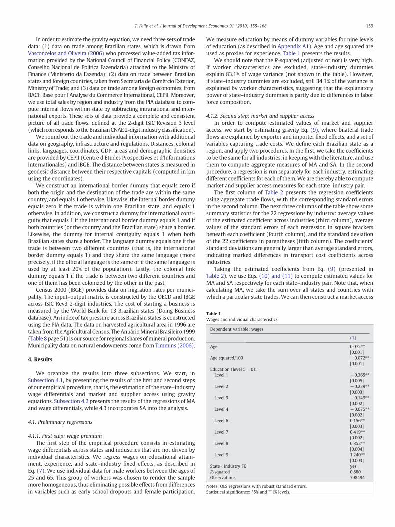
Table 1Wages and individual characteristics.

Dependent variable: wages

(1)

Age 0.072⁎⁎[0.001]

Age squared/100 −0.072⁎⁎[0.001]

Education (level 5=0):Level 1 −0.365⁎⁎

[0.005]Level 2 −0.239⁎⁎

[0.003]Level 3 −0.149⁎⁎

[0.002]Level 4 −0.075⁎⁎

[0.002]Level 6 0.156⁎⁎

[0.003]Level 7 0.419⁎⁎

[0.002]Level 8 0.852⁎⁎

[0.004]Level 9 1.240⁎⁎

[0.003]State×industry FE yesR-squared 0.880Observations 798494

Notes: OLS regressions with robust standard errors.Statistical significance: *5% and **1% levels.


In order to estimate the gravity equation, we need three sets of tradedata: (1) data on trade among Brazilian states, which is drawn fromVasconcelos and Oliveira (2006) who processed value-added tax infor-mation provided by the National Council of Financial Policy (CONFAZ,Conselho Nacional de Politica Fazendaria) attached to the Ministry ofFinance (Ministerio da Fazenda); (2) data on trade between Brazilianstates and foreign countries, taken from Secretaria de Comércio Exterior,Ministry of Trade; and (3) data on trade among foreign economies, fromBACI: Base pour l'Analyse du Commerce International, CEPII. Moreover,we use total sales by region and industry from the PIA database to com-pute internal flows within state by subtracting intranational and inter-national exports. These sets of data provide a complete and consistentpicture of all trade flows, defined at the 2-digit ISIC Revision 3 level(which corresponds to theBrazilianCNAE2-digit industry classification).

We round out the trade and individual informationwith additionaldata on geography, infrastructure and regulations. Distances, coloniallinks, languages, coordinates, GDP, areas and demographic densitiesare provided by CEPII (Centre d'Etudes Prospectives et d'InformationsInternationales) and IBGE. The distance between states is measured ingeodesic distance between their respective capitals (computed in kmusing the coordinates).

We construct an international border dummy that equals zero ifboth the origin and the destination of the trade are within the samecountry, and equals 1 otherwise. Likewise, the internal border dummyequals zero if the trade is within one Brazilian state, and equals 1otherwise. In addition, we construct a dummy for international conti-guity that equals 1 if the international border dummy equals 1 and ifboth countries (or the country and the Brazilian state) share a border.Likewise, the dummy for internal contiguity equals 1 when bothBrazilian states share a border. The language dummy equals one if thetrade is between two different countries (that is, the internationalborder dummy equals 1) and they share the same language (moreprecisely, if the official language is the same or if the same language isused by at least 20% of the population). Lastly, the colonial linkdummy equals 1 if the trade is between two different countries andone of them has been colonized by the other in the past.

Census 2000 (IBGE) provides data on migration rates per munici-pality. The input–output matrix is constructed by the OECD and IBGEacross ISIC Rev3 2-digit industries. The cost of starting a business ismeasured by the World Bank for 13 Brazilian states (Doing Businessdatabase). An index of tax pressure across Brazilian states is constructedusing the PIA data. The data on harvested agricultural area in 1996 aretaken from theAgricultural Census. TheAnuárioMineral Brasileiro 1999(Table 8 page 51) is our source for regional shares ofmineral production.Municipality data on natural endowments come from Timmins (2006).

4. Results

We organize the results into three subsections. We start, inSubsection 4.1, by presenting the results of the first and second stepsof our empirical procedure, that is, the estimation of the state–industrywage differentials and market and supplier access using gravityequations. Subsection 4.2 presents the results of the regressions of MAand wage differentials, while 4.3 incorporates SA into the analysis.

4.1. Preliminary regressions

4.1.1. First step: wage premiumThe first step of the empirical procedure consists in estimating

wage differentials across states and industries that are not driven byindividual characteristics. We regress wages on educational attain-ment, experience, and state–industry fixed effects, as described inEq. (7). We use individual data for male workers between the ages of25 and 65. This group of workers was chosen to render the samplemore homogeneous, thus eliminating possible effects from differencesin variables such as early school dropouts and female participation.

We measure education by means of dummy variables for nine levelsof education (as described in Appendix A1). Age and age squared areused as proxies for experience. Table 1 presents the results.

We should note that the R-squared (adjusted or not) is very high.If worker characteristics are excluded, state–industry dummiesexplain 83.1% of wage variance (not shown in the table). However,if state–industry dummies are excluded, still 34.1% of the variance isexplained by worker characteristics, suggesting that the explanatorypower of state–industry dummies is partly due to differences in laborforce composition.

4.1.2. Second step: market and supplier accessIn order to compute estimated values of market and supplier

access, we start by estimating gravity Eq. (9), where bilateral tradeflows are explained by exporter and importer fixed effects, and a set ofvariables capturing trade costs. We define each Brazilian state as aregion, and apply two procedures. In the first, we take the coefficientsto be the same for all industries, in keepingwith the literature, and usethem to compute aggregate measures of MA and SA. In the secondprocedure, a regression is run separately for each industry, estimatingdifferent coefficients for each of them.We are thereby able to computemarket and supplier access measures for each state–industry pair.

The first column of Table 2 presents the regression coefficientsusing aggregate trade flows, with the corresponding standard errorsin the second column. The next three columns of the table show somesummary statistics for the 22 regressions by industry: average valuesof the estimated coefficient across industries (third column), averagevalues of the standard errors of each regression in square bracketsbeneath each coefficient (fourth column), and the standard deviationof the 22 coefficients in parentheses (fifth column). The coefficients'standard deviations are generally larger than average standard errors,indicating marked differences in transport cost coefficients acrossindustries.

Taking the estimated coefficients from Eq. (9) (presented inTable 2), we use Eqs. (10) and (11) to compute estimated values forMA and SA respectively for each state–industry pair. Note that, whencalculating MA, we take the sum over all states and countries withwhich a particular state trades. We can then construct a market access

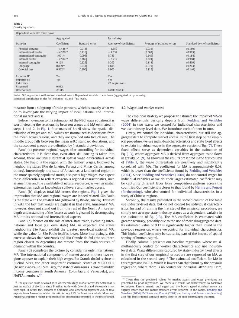
Table 2Gravity equations.

Dependent variable: trade flows

Aggregated By industry

Statistics Coefficient Standard error Average of coefficients Average of standard errors Standard dev. of coefficients

Physical distance −1.448⁎⁎ [0.018] −1.359 [0.031] (0.180)International border −4.326⁎⁎ [0.116] −4.534 [0.563] (0.983)International contiguity 1.001⁎⁎ [0.095] 0.785 [0.249] (0.184)Internal border −2.594⁎⁎ [0.386] −3.212 [0.224] (0.968)Internal contiguity 0.128 [0.225] 0.205 [0.118] (0.469)Language 0.839⁎⁎ [0.043] 0.604 [0.071] (0.263)Colonial link 0.832⁎⁎ [0.100] 0.903 [0.115] (0.140)

Exporter FE Yes YesImporter FE Yes YesIndustries 22 RegressionsR-squared 0.982Observations 25315 Total: 246833

Notes: OLS regressions with robust standard errors. Dependent variable: trade flows (aggregated or by industry).Statistical significance in the first column: *5% and **1% levels.


measure from a subgroup of trade partners, which is exactly what wedo to investigate the varying impact of local, national and interna-tional market access.

Before moving on to the estimation of the NEG wage equation, it isworth viewing the relationship between wages and MA estimated insteps 1 and 2. In Fig. 1, four maps of Brazil show the spatial dis-tribution of wages and MA. Values are normalized as deviations fromthe mean across regions, and they are grouped into five classes. Themiddle group falls between the mean ±0.5 standard deviations, andthe subsequent groups are delimited by 1 standard deviation.

Panel (a) presents regional wages after controlling for individualcharacteristics. It is clear that, even after skill sorting is taken intoaccount, there are still substantial spatial wage differentials acrossstates. São Paulo is the region with the highest wages, followed byneighboring states (Rio de Janeiro, Paraná and Minas Gerais, amongothers). Interestingly, the state of Amazonas, a landlocked region inthe more sparsely populated north, also posts high wages. We expectthese differentials to reflect exogenous regional characteristics, suchas amenities and the availability of natural resources, as well as spatialexternalities, such as knowledge spillovers and market access.

Panel (b) displays total MA across the regions. Fig. 1 gives theimpression that MA and regional wages are indeed related. São Paulois the state with the greatest MA (followed by Rio de Janeiro). This tiesin with the fact that wages are highest in that state. Amazonas' MA,however, does not stand out from the rest of the North. A more in-depth understanding of the factors at work is gleaned by decomposingMA into its national and international aspects.

Panel (c) focuses on the role of inter-state trade, excluding inter-national and local (i.e. own state) MA. As expected, the statesneighboring São Paulo exhibit the greatest non-local national MA,while the value for São Paulo itself is lower. More interestingly, thisexercise shows that Amazonas and Rio Grande do Sul (the southernregion closest to Argentina) are remote from the main sources ofdemand within the country.

Panel (d) completes the picture by considering only internationalMA. The international component of market access in these two re-gions appears to explain their highwages. Rio Grande do Sul is close toBuenos Aires, the other important economic center of MERCOSUR(besides São Paulo). Similarly, the state of Amazonas is close tomiddleincome countries in South America (Colombia and Venezuela), andNAFTA members.15

15 The question could be asked as to whether this high market access for Amazonas isjust an artifact of the data, since Brazilian trade with Colombia and Venezuela is notvery high. In actual fact, exports to Colombia and Venezuela represent 20% of totalexports from Amazonas, while this ratio is only 2.4% for Brazil as a whole. Moreover,Amazonas exports a higher proportion of its production compared to the rest of Brazil.

4.2. Wages and market access

The empirical strategywe propose to estimate the impact of MA onwage differentials basically departs from Redding and Venables(2004) in two ways: we control for individual characteristics andwe use industry-level data. We introduce each of them in turn.

Firstly, we control for individual characteristics, but still use ag-gregate data to compute market access. In the first step of the empir-ical procedure, we use individual characteristics and state fixed effectsto explain individual wages in the aggregate version of Eq. (7). Thesefixed effects serve as dependent variables in the estimation ofEq. (13), where aggregate MA is derived from aggregate trade flowsin gravity Eq. (9). As shown in the results presented in the first columnof Table 3, the wage differentials are positively and significantlycorrelated with MA. The coefficient for MA is approximately 0.08,which is lower than the coefficients found by Redding and Venables(2004). Since Redding and Venables (2004) do not control wages forindividual variables as we do, their larger estimated coefficient maybe capturing different labor force composition patterns across thecountries. Our coefficient is closer to that found by Hering and Poncet(forthcoming), who also control for individual characteristics in astudy of Chinese regions.

Secondly, the results presented in the second column of the tableuse industry-level data, but do not control for individual character-istics. Instead of running the first step of the empirical procedure, wesimply use average state–industry wages as a dependent variable inthe estimation of Eq. (13). The MA coefficient is estimated withgreater accuracy, probably due to the use of more disaggregated data.Its estimated value of 0.17 is significantly higher than found in theprevious regression, where we control for individual characteristics.This higher coefficient may be capturing part of the impact of spatialsorting of human capital.

Finally, column 3 presents our baseline regression, where we si-multaneously control for worker characteristics and use industry-level data. Wage differentials captured by state–industry fixed effectsin the first step of our empirical procedure are regressed on MA, ascalculated in the second step.16 The estimated coefficient for MA inthis regression is 0.14, which is lower than that found by the previousregression, where there is no control for individual attributes. Here,

16 Given that the predicted values for market access and wage premiums aregenerated by prior regressions, we check our results for sensitiveness to bootstraptechniques. Results remain unchanged and the bootstrapped standard errors areslightly lower than the robust standard errors reported in the Tables. Redding andVenables (2004), De Sousa and Poncet (2007) and Hering and Poncet (forthcoming)also find bootstrapped standard errors close to the non-bootstrapped estimate.

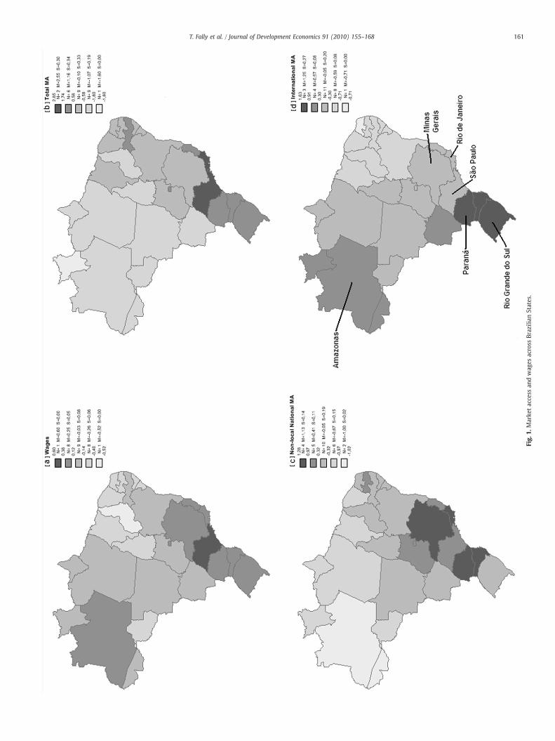
Fig.

1.Marke

taccess

andwag

esacross

Brazilian

States.


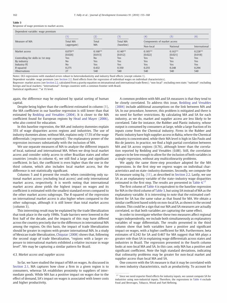
Table 3Response of wage premium to market access.

Dependent variable: wage premium

(1) (2) (3) (4) (5) (6)

Measure of MA Total MA(aggregate)

TotalMA

Total MA(baseline)

Components of market access

Non-local National International

Market access 0.079⁎⁎ 0.168⁎⁎ 0.140⁎⁎ 0.185⁎⁎ 0.162⁎⁎ 0.228⁎⁎[0.026] [0.013] [0.012] [0.022] [0.021] [0.018]

Controlling for skills in 1st step Yes No Yes Yes Yes YesBy industry No Yes Yes Yes Yes YesIndustry FE No Yes Yes Yes Yes YesR-squared 0.275 0.432 0.350 0.255 0.248 0.294Observations 27 540 540 540 540 540

Notes: OLS regressions with standard errors robust to heteroskedasticity and industry fixed effects (except column 1).Dependent variable: wage premium (see Section 2.2, fixed effects from the regression of individual wages on individual characteristics).Regressor: market access (see Section 2.2, calculated from a gravity equation on intranational and international trade flows); “non-local”: excluding own state; “national“: excludingforeign and local markets; “international”: foreign countries with a common frontier with Brazil.Statistical significance: **at 1% level.

17 Since we need exporter fixed effects for industry inputs, we cannot compute SA forindustries using non-industrial inputs. Therefore, the regressions in Table 4 excludeFood and Beverages, Tobacco, Wood and Fuel Refining.


again, the difference may be explained by spatial sorting of humancapital.

Despite being higher than the coefficient estimated in column (1),the MA coefficient in our baseline regression is still lower than thatestimated by Redding and Venables (2004). It is closer to the MAcoefficient found for European regions by Head and Mayer (2006),who also control for education.

In this baseline regression, the MA and industry dummies explain35% of wage disparities across regions and industries. The use ofindustry dummies alone, withoutMA, explains only 17.5% of the wagedifferentials (regression not reported): The explanatory power of theregression increases substantially with the inclusion of MA.

We use separate measures of MA to analyze the different impactsof local, national and international MA. When we drop local marketaccess and consider solely access to other Brazilian states and othercountries (results in column 4), we still find a large and significantcoefficient. In fact, the coefficient is even higher than the one in thethird column, which also includes local market access, but thedifference is not statistically significant.

Columns 5 and 6 present the results when considering only na-tional market access (excluding local access) and only internationalmarket access, respectively. It is worth noting that internationalmarket access alone yields the highest impact on wages and itscoefficient is estimated with the smallest standard errors compared tothe other market access subgroups. The R-squared of the regressionon international market access is also higher when compared to theother subgroups, although it is still lower than total market access(column 3).

This interesting result may be explained by the trade liberalizationthat took place in the early 1990s. Trade barriers were lowered in thefirst half of the decade, and the impacts of this may have differedacross the country precisely due to the differences in international MAamong the regions. On this basis, the impact of trade liberalizationshould be greater in regions with greater international MA. In a studyof Mexican trade liberalization, Chiquiar (2008) shows that, followingthe second stage of trade liberalization, “regions with a larger ex-posure to international markets exhibited a relative increase in wagelevel”. We may be capturing a similar pattern for Brazil.

4.3. Market access and supplier access

So far, we have studied the impact of MA onwages. As discussed inSection 2.1, MA captures how close a firm in a given region is toconsumers, whereas SA establishes proximity to suppliers of inter-mediate goods. While MA has a positive impact on wages due to theeffect of demand, SA's impact on wages is associated with lower costsand higher productivity.

A common problem with MA and SA measures is that they tend tobe closely correlated. To address this issue, Redding and Venables(2004) include additional assumptions on the link between MA andSA. In our procedure, however, this problem is mitigated and there isno need for further restrictions. By calculating MA and SA for eachindustry, as we do, market and supplier access are less likely to becorrelated. Take for instance, the Rubber and Plastic industry, whoseoutput is consumed by consumers at large, while a large fraction of itsinputs come from the Chemical industry. Firms in the Rubber andPlastic industry have high supplier access in Bahia,where the Chemicalindustry is concentrated, while their MA level is high in São Paulo andRio de Janeiro. In practice, we find a high partial correlation betweenMA and SA across regions (0.76), although lower than the correla-tion reported by Redding and Venables (0.88). Still, the correlationappears to be low enough to allow for the inclusion of both variables ina single regression, without any multicolinearity problems.

We apply the same three-step procedure adopted for the MAregressions. In the first step we regress wages on individual char-acteristics and on state–industry dummies. Secondly, we compute theSA measure using Eq. (11), as described in Section 2.2. Lastly, we useSA as an explanatory variable of the state–industry wage disparitiesestimated in the first step. The results are presented in Table 4.17

The first column of Table 4 is equivalent to the baseline regressionforMA in the third column of Table 3, but using SA instead ofMA as theexplanatory variable. It is interesting to note that the estimated coef-ficient for SA has the same value as that found for MA. We obtain asimilar coefficient based solely onnon-local SA, as shown in the secondcolumn. This could be a sign that ourMA and SAmeasures are actuallycorrelated, so that both variables are capturing the same effect.

In order to investigate whether these two measures affect regionalwages independently, we include both simultaneously as explanatoryvariables of wage differentials. The results presented in the thirdcolumn show that both variables have a positive and significantimpact on wages, with a higher coefficient for MA. Furthermore, betaestimates of 0.242 for SA and 0.467 for MA suggest that MA plays agreater role than SA in explaining wage differentials across states andindustries in Brazil. The regression presented in the fourth columnlooks at non-local MA and SA. In this case, only MA has a positive andsignificant coefficient. Note the high standard deviations, indicatingthat colinearity problems may be greater for non-local market andsupplier access than local MA and SA.

One concern with the SA measure is that it may be correlated withits own industry characteristics, such as productivity. To account for

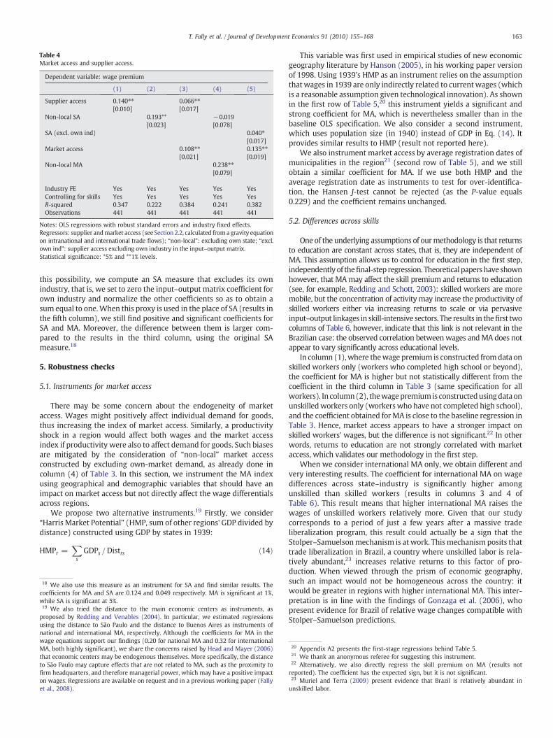
Table 4Market access and supplier access.


(1) (2) (3) (4) (5)

Supplier access 0.140⁎⁎ 0.066⁎⁎[0.010] [0.017]

Non-local SA 0.193** −0.019[0.023] [0.078]

SA (excl. own ind) 0.040⁎[0.017]

Market access 0.108⁎⁎ 0.135⁎⁎[0.021] [0.019]

Non-local MA 0.238⁎⁎[0.079]

Industry FE Yes Yes Yes Yes YesControlling for skills Yes Yes Yes Yes YesR-squared 0.347 0.222 0.384 0.241 0.382Observations 441 441 441 441 441

Notes: OLS regressions with robust standard errors and industry fixed effects.Regressors: supplier andmarket access (see Section 2.2, calculated froma gravity equationon intranational and international trade flows); “non-local”: excluding own state; “excl.own ind”: supplier access excluding own industry in the input–output matrix.Statistical significance: *5% and **1% levels.


this possibility, we compute an SA measure that excludes its ownindustry, that is, we set to zero the input–output matrix coefficient forown industry and normalize the other coefficients so as to obtain asum equal to one.When this proxy is used in the place of SA (results inthe fifth column), we still find positive and significant coefficients forSA and MA. Moreover, the difference between them is larger com-pared to the results in the third column, using the original SAmeasure.18

5. Robustness checks

5.1. Instruments for market access

There may be some concern about the endogeneity of marketaccess. Wages might positively affect individual demand for goods,thus increasing the index of market access. Similarly, a productivityshock in a region would affect both wages and the market accessindex if productivity were also to affect demand for goods. Such biasesare mitigated by the consideration of “non-local” market accessconstructed by excluding own-market demand, as already done incolumn (4) of Table 3. In this section, we instrument the MA indexusing geographical and demographic variables that should have animpact on market access but not directly affect the wage differentialsacross regions.

We propose two alternative instruments.19 Firstly, we consider“Harris Market Potential” (HMP, sum of other regions' GDP divided bydistance) constructed using GDP by states in 1939:

HMPr =Xs

GDPs =Distrs ð14Þ

18 We also use this measure as an instrument for SA and find similar results. Thecoefficients for MA and SA are 0.124 and 0.049 respectively. MA is significant at 1%,while SA is significant at 5%.19 We also tried the distance to the main economic centers as instruments, asproposed by Redding and Venables (2004). In particular, we estimated regressionsusing the distance to São Paulo and the distance to Buenos Aires as instruments ofnational and international MA, respectively. Although the coefficients for MA in thewage equations support our findings (0.20 for national MA and 0.32 for internationalMA, both highly significant), we share the concerns raised by Head and Mayer (2006)that economic centers may be endogenous themselves. More specifically, the distanceto São Paulo may capture effects that are not related to MA, such as the proximity tofirm headquarters, and therefore managerial power, which may have a positive impacton wages. Regressions are available on request and in a previous working paper (Fallyet al., 2008).

This variable was first used in empirical studies of new economicgeography literature by Hanson (2005), in his working paper versionof 1998. Using 1939's HMP as an instrument relies on the assumptionthat wages in 1939 are only indirectly related to currentwages (whichis a reasonable assumption given technological innovation). As shownin the first row of Table 5,20 this instrument yields a significant andstrong coefficient for MA, which is nevertheless smaller than in thebaseline OLS specification. We also consider a second instrument,which uses population size (in 1940) instead of GDP in Eq. (14). Itprovides similar results to HMP (result not reported here).

We also instrument market access by average registration dates ofmunicipalities in the region21 (second row of Table 5), and we stillobtain a similar coefficient for MA. If we use both HMP and theaverage registration date as instruments to test for over-identifica-tion, the Hansen J-test cannot be rejected (as the P-value equals0.229) and the coefficient remains unchanged.

5.2. Differences across skills

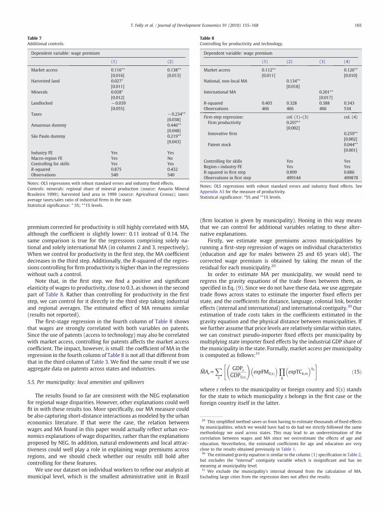
One of the underlying assumptions of ourmethodology is that returnsto education are constant across states, that is, they are independent ofMA. This assumption allows us to control for education in the first step,independently of thefinal-step regression. Theoretical papershave shownhowever, that MAmay affect the skill premium and returns to education(see, for example, Redding and Schott, 2003): skilled workers are moremobile, but the concentration of activity may increase the productivity ofskilled workers either via increasing returns to scale or via pervasiveinput–output linkages in skill-intensive sectors. The results in thefirst twocolumns of Table 6, however, indicate that this link is not relevant in theBrazilian case: the observed correlation betweenwages andMA does notappear to vary significantly across educational levels.

In column (1),where thewage premium is constructed fromdata onskilled workers only (workers who completed high school or beyond),the coefficient for MA is higher but not statistically different from thecoefficient in the third column in Table 3 (same specification for allworkers). In column(2), thewagepremiumis constructedusingdataonunskilledworkers only (workerswho have not completed high school),and the coefficient obtained forMA is close to the baseline regression inTable 3. Hence, market access appears to have a stronger impact onskilled workers' wages, but the difference is not significant.22 In otherwords, returns to education are not strongly correlated with marketaccess, which validates our methodology in the first step.

When we consider international MA only, we obtain different andvery interesting results. The coefficient for international MA on wagedifferences across state–industry is significantly higher amongunskilled than skilled workers (results in columns 3 and 4 ofTable 6). This result means that higher international MA raises thewages of unskilled workers relatively more. Given that our studycorresponds to a period of just a few years after a massive tradeliberalization program, this result could actually be a sign that theStolper–Samuelsonmechanism is at work. Thismechanism posits thattrade liberalization in Brazil, a country where unskilled labor is rela-tively abundant,23 increases relative returns to this factor of pro-duction. When viewed through the prism of economic geography,such an impact would not be homogeneous across the country: itwould be greater in regions with higher international MA. This inter-pretation is in line with the findings of Gonzaga et al. (2006), whopresent evidence for Brazil of relative wage changes compatible withStolper–Samuelson predictions.

20 Appendix A2 presents the first-stage regressions behind Table 5.21 We thank an anonymous referee for suggesting this instrument.22 Alternatively, we also directly regress the skill premium on MA (results notreported). The coefficient has the expected sign, but it is not significant.23 Muriel and Terra (2009) present evidence that Brazil is relatively abundant inunskilled labor.

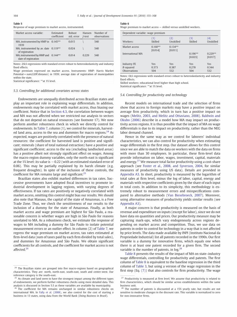
Table 6Wage premium to market access — skilled versus unskilled workers.


(1) (2) (3) (4)Workers: Skilled Unskilled Skilled Unskilled

Market access 0.160⁎⁎ 0.134⁎⁎[0.014] [0.011]

International MA 0.196⁎⁎ 0.229⁎⁎[0.023] [0.017]

Industry FE Yes Yes Yes YesR-squared 0.373 0.387 0.278 0.344Observations 504 532 504 532

Notes: OLS regressions with standard errors robust to heteroskedasticity and industryfixed effects.Skilled workers: educational level higher than high school.Statistical significance: **at 1% level.

Table 5Response of wage premium to market access, instrumented.

Market access variable: Estimatedcoefficient

Robuststd. error

HansenJ-test

Number ofobservations

MA, instrumented by HMP in1939

0.145⁎⁎ 0.015 \ 540

MA, instrumented by av. dateof registration

0.119⁎⁎ 0.024 \ 540

MA, instrumentedbyHMPanddate of registration

0.144⁎⁎ 0.014 0.229 540

Notes: 2SLS regressions with standard errors robust to heteroskedasticity and industryfixed effects.Wage premium regressed on market access. Instruments: HMP: Harris MarketPotential=sum(GDP/distance) in 1939; average date of registration of municipalitieswithin the state.Statistical significance: **at 1% level.


5.3. Controlling for additional covariates across states

Endowments are unequally distributed across Brazilian states andplay an important role in explaining wage differentials. In addition,endowments may be correlated with market access, thus biasing ourcoefficient. Notice that in Section 4.3, the correlation between wagesand MA was not affected when we restricted our analysis to sectorsthat do not depend on natural resources (see footnote 17). We nowperform another robustness check in which we directly control forendowments. In Table 7, column (1), we control for minerals, harvest-ed land area, access to the sea and dummies for macro regions.24 Asexpected, wages are positively correlated with the presence of naturalresources: the coefficient for harvested land is positive and signifi-cant; minerals (share of total national extraction) have a positive andsignificant coefficient; access to the sea (excluding landlocked areas)has a positive albeit not strongly significant effect on wages. Amongthe macro-region dummy variables, only the north-east is significantat the 1% level: its value is−0.22 (with an estimated standard error of0.06). This may be partially explained by its harsh climate (e.g.frequent droughts). In spite of the inclusion of these controls, thecoefficient for MA remains large and significant.25

Brazilian states also exhibit marked differences in tax rates. Suc-cessive governments have adopted fiscal incentives to promote in-dustrial development in lagging regions, with varying degrees ofeffectiveness. If tax rates are positively or negatively correlated withmarket access, omitting this control might bias our results. We shouldalso note that Manaus, the capital of the state of Amazonas, is a FreeTrade Zone. Thus, we check the sensitiveness of our results to theinclusion of a dummy for the state of Amazonas. Finally, as bothmarket access and wage premium are highest for São Paulo, a rea-sonable concern is whether wages are high in São Paulo for reasonsunrelated to MA. As a robustness check, we estimate the response ofwages to MA including a dummy for São Paulo to isolate potentialmeasurement errors or an outlier effect. In column (2) of Table 7, weregress the wage premium on market access, tax rates estimated atfirm-level data (sum of taxes paid by each firm divided by total sales),and dummies for Amazonas and São Paulo. We obtain significantcoefficients for all controls, and the coefficient for market access is notaffected.26

24 The Brazilian states are grouped into five macro-regions based on geographicalcharacteristics. They are: north, north-east, south-east, south and center-west. Ourreference category is the south-east.25 As climate and land seem to have the strongest impact among the different typesof endowments, we perform further robustness checks using more detailed data. Thisanalysis is discussed in Section 5.5 as these variables are available by municipality.26 The coefficient for MA remains unchanged in similar robustness checks oninternational MA. In Fally et al. (2008), we also control for the cost of starting abusiness in 13 states, using data from the World Bank (Doing Business in Brazil).

5.4. Controlling for productivity and technology

Recent models on international trade and the selection of firmsshow that access to foreign markets may have a positive impact onaverage firm productivity, which in turn has a positive impact onwages (Melitz, 2003, and Melitz and Ottaviano, 2008). Baldwin andOkubo (2006) describe in a model how MA may impact on produc-tivity across regions. It is thus possible that the impact of MA on wagedifferentials is due to its impact on productivity, rather than the NEGlabor demand channel.

Hence in the same way as we control for laborers' individualcharacteristics, we can also control for productivity when estimatingwage differentials in the first step. Our dataset allows for this controlsince we are able to match the data on workers with the data on firmswith more than 30 employees. In particular, these firm-level dataprovide information on labor, wages, investment, capital, materialsand energy.27 We measure total factor productivity using a cost-shareapproach (see Foster et al., 2008, and Syverson, 2004, for similarmeasures of productivity using US data). Details are provided inAppendix A3. In short, productivity is measured by the logarithm oftotal sales at firm level, minus the log of labor, capital, energy andmaterials with respective coefficients given by the share of each inputin total costs. In addition to its simplicity, this methodology is ex-tremely robust to measurement errors and misspecifications com-pared to alternative methods (Van Biesebroeck, 2007). Moreover,using alternative measures of productivity yields similar results (seeAppendix A3).

A major concern is that productivity is measured on the basis ofrevenue and expenditure on inputs (except for labor), since we do nothave data on quantities and prices. Our productivity measure may becapturing mark-ups, which vary endogenously across regions de-pending on market access and competition. Thus, we use data onpatents in order to control for technology in a way that is not affectedby price levels. The data made available by INPI (Instituto Nacional daPropriedade Industrial) list all patents recorded in the 1990s. Our firstvariable is a dummy for innovative firms, which equals one whenthere is at least one patent recorded for a given firm. The secondvariable is the number of patents, in log.28

Table 8 presents the results of the impact of MA on state–industrywage differentials, controlling for productivity and patents. The firstcolumn of Table 8 is equivalent to the baseline regression in the thirdcolumn of Table 3, but using a version of the wage regression in thefirst step (Eq. (7)) that also controls for firm productivity. The wage

27 Productivity is measured at firm level. We assume that productivity is related tofirm characteristics, which should be similar across establishments within the samebusiness unit.28 The number of patents is discounted at a 15% yearly rate, but results are notsensitive to moderate changes in the discount rate. This variable is normalized to zerofor non-innovative firms.

29 This simplified method saves us from having to estimate thousands of fixed effectsby municipalities, which we would have had to do had we strictly followed the samemethodology we used across states. This may lead to an underestimation of thecorrelation between wages and MA since we overestimate the effects of age andeducation. Nevertheless, the estimated coefficients for age and education are veryclose to the results obtained previously in Table 1.30 The estimated gravity equation is similar to the column (1) specification in Table 2,but excludes the “internal” contiguity variable which is insignificant and has nomeaning at municipality level.31 We exclude the municipality’s internal demand from the calculation of MA.Excluding large cities from the regression does not affect the results.

Table 7Additional controls.


(1) (2)

Market access 0.116** 0.138**[0.016] [0.013]

Harvested land 0.027*[0.011]

Minerals 0.028*[0.012]

Landlocked −0.039[0.055]

Taxes −0.234**[0.038]

Amazonas dummy 0.446**[0.048]

São Paulo dummy 0.219**[0.043]

Industry FE Yes YesMacro-region FE Yes NoControlling for skills Yes YesR-squared 0.875 0.432Observations 540 540

Notes: OLS regressions with robust standard errors and industry fixed effects.Controls: minerals: regional share of mineral production (source: Anuario MineralBrasileiro 1999); harvested land area in 1999 (source: Agricultural Census); taxes:average taxes/sales ratio of industrial firms in the state.Statistical significance: * 5%; **1% levels.

Table 8Controlling for productivity and technology.


(1) (2) (3) (4)

Market access 0.112** 0.126**[0.011] [0.010]

National, non-local MA 0.134**[0.018]

International MA 0.201**[0.017]

R-squared 0.403 0.328 0.388 0.343Observations 466 466 466 534

First-step regression: col. (1)–(3) col. (4)Firm productivity 0.297**

[0.002]Innovative firm 0.259**

[0.002]Patent stock 0.044**

[0.001]

Controlling for skills Yes YesRegion×industry FE Yes YesR-squared in first step 0.899 0.886Observations in first step 499144 499878

Notes: OLS regressions with robust standard errors and industry fixed effects. SeeAppendix A3 for the measure of productivity.Statistical significance: *5% and **1% levels.


premium corrected for productivity is still highly correlated with MA,although the coefficient is slightly lower: 0.11 instead of 0.14. Thesame comparison is true for the regressions comprising solely na-tional and solely international MA (in columns 2 and 3, respectively).When we control for productivity in the first step, the MA coefficientdecreases in the third step. Additionally, the R-squared of the regres-sions controlling for firm productivity is higher than in the regressionswithout such a control.

Note that, in the first step, we find a positive and significantelasticity of wages to productivity, close to 0.3, as shown in the secondpart of Table 8. Rather than controlling for productivity in the firststep, we can control for it directly in the third step taking industrialand regional averages. The estimated effect of MA remains similar(results not reported).

The first-stage regression in the fourth column of Table 8 showsthat wages are strongly correlated with both variables on patents.Since the use of patents (access to technology) may also be correlatedwith market access, controlling for patents affects the market accesscoefficient. The impact, however, is small: the coefficient of MA in theregression in the fourth column of Table 8 is not all that different fromthat in the third column of Table 3. We find the same result if we useaggregate data on patents across states and industries.

5.5. Per municipality: local amenities and spillovers

The results found so far are consistent with the NEG explanationfor regional wage disparities. However, other explanations could wellfit in with these results too. More specifically, our MA measure couldbe also capturing short-distance interactions as modeled by the urbaneconomics literature. If that were the case, the relation betweenwages and MA found in this paper would actually reflect urban eco-nomics explanations of wage disparities, rather than the explanationsproposed by NEG. In addition, natural endowments and local attrac-tiveness could well play a role in explaining wage premiums acrossregions, and we should check whether our results still hold aftercontrolling for these features.

We use our dataset on individual workers to refine our analysis atmunicipal level, which is the smallest administrative unit in Brazil

(firm location is given by municipality). Honing in this way meansthat we can control for additional variables relating to these alter-native explanations.

Firstly, we estimate wage premiums across municipalities byrunning a first-step regression of wages on individual characteristics(education and age for males between 25 and 65 years old). Thecorrected wage premium is obtained by taking the mean of theresidual for each municipality.29

In order to estimate MA per municipality, we would need toregress the gravity equations of the trade flows between them, asspecified in Eq. (9). Since we do not have these data, we use aggregatetrade flows across states to estimate the importer fixed effects perstate, and the coefficients for distance, language, colonial link, bordereffects (internal and international) and international contiguity.30 Ourestimation of trade costs takes in the coefficients estimated in thegravity equation and the physical distance between municipalities. Ifwe further assume that price levels are relatively similar within states,we can construct pseudo-importer fixed effects per municipality bymultiplying state importer fixed effects by the industrial GDP share ofthemunicipality in the state. Formally, market access per municipalityis computed as follows:31

MAruXs

GDPsGDPS sð Þ

!expFMS sð Þ� �Y

k

expTCk;rs

� �δk" #ð15Þ

where s refers to the municipality or foreign country and S(s) standsfor the state to which municipality s belongs in the first case or theforeign country itself in the latter.

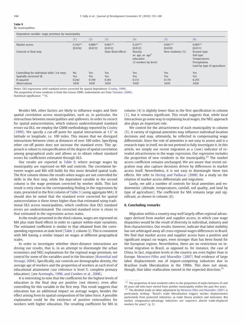
Table 9By municipalities.

Dependent variable: wage premium by municipality

(1) (2) (3) (4) (5) (6)

Market access 0.162⁎⁎ 0.086⁎⁎ 0.091⁎⁎ 0.107⁎⁎ 0.091⁎⁎ 0.095⁎⁎[0.016] [0.013] [0.012] [0.012] [0.010] [0.011]

Controls in final step State fixed effects Density New residents (%) Erosion typeav. age, av. age2 Soil typeeducation Temperatures(% workers by level) Precipitation

Land by type of agriculture

Controlling for individual skills (1st step) No Yes Yes Yes Yes YesSpatially corrected SE Yes Yes Yes Yes Yes YesR-squared 0.242 0.109 0.301 0.151 0.170 0.255Observations 3439 3439 3439 3439 3439 3439

Notes: OLS regressions with standard errors corrected for spatial dependence (Conley, 1999).The proportion of new residents is from the Census 2000; endowments are from Timmins (2006).Statistical significance: **1%.

32 The proportion of new residents refers to the proportion of males between 25 and65 years old who have moved from another municipality within the past five years.33 The detailed study on labor adjustment by Menezes-Filho and Muendler (2007) isparticularly striking: “Brazil's trade liberalization triggers worker displacementsparticularly from protected industries, as trade theory predicts and welcomes. Butneither comparative-advantage industries nor exporters absorb trade-displacedworkers for years” (p. 2).


Besides MA, other factors are likely to influence wages and theirspatial correlation across municipalities, such as, in particular, theinteractions between municipalities and spillovers. In order to correctfor spatial autocorrelation, which induces underestimated standarderrors via OLS, we employ the GMMmethodology reported by Conley(1999). We specify a cut-off point for spatial interactions at 1.5° inlatitude or longitude, i.e. 100 miles. This means that we disregardinteractions between cities at distances of over 100 miles. Specifyingother cut-off points does not increase the standard error. This ap-proach is robust to misspecification of the degree of spatial correlationamong geographical units and allows us to obtain robust standarderrors for coefficients estimated through OLS.

Our results are reported in Table 9, where average wages bymunicipality are regressed on MA and controls. The correlation be-tween wages and MA still holds for this more detailed spatial scale.The first column shows the results when wages are not controlled forskills in the first step, while the dependent variable in the secondcolumn is the wage premium corrected by worker skills. This lastresult is very close to the corresponding finding in the regressions bystate, presented in the first column of Table 3 (using aggregate MA). Itshould also be noted that the standard error corrected for spatialautocorrelation is three times higher than that estimated using tradi-tional OLS across municipalities, which confirms that OLS standarderrors are underestimated. The corrected standard error is closer tothat estimated in the regressions across states.

In the results presented in the third column, wages are regressed onMA plus state fixed effects in order to capture within-state variations.The estimated coefficient is similar to that obtained from the corre-sponding regression at state level (Table 3, column 3). This is consistentwith MA having a similar impact on wages at different geographicalscales.

In order to investigate whether short-distance interactions aredriving our results, that is, in an attempt to disentangle the urbaneconomics and NEG explanations for the regional wage premium, wecontrol for some of the variables used in the literature (Rosenthal andStrange, 2004). Specifically, our controls are demographic density, theaverage age of workers and the proportion of workers at each level ofeducational attainment (our reference is level 5: complete primaryeducation) (see Acemoglu, 1996, and Combes et al., 2008).

It is interesting to note that the coefficients for the highest levels ofeducation in the final step are positive (not shown), even aftercontrolling for this variable in the first step. This result suggests thateducation has an additional impact on average wages, besides theeffect arising from its spatial composition of the labor force. A possibleexplanation could be the existence of positive externalities forworkers with higher education. The resulting coefficient for MA in

column (4) is slightly lower than in the first specification in column(1), but it remains significant. This result suggests that, while localinteractions go someway to explaining local wages, the NEG approachalso plays an important role.

We control for the attractiveness of each municipality in column(5). A variety of regional amenities may influence individual locationdecisions and may, ultimately, be reflected in compensating wagedifferentials. Since the role of amenities is not easy to assess and is aresearch topic in itself, we do not pretend to fully investigate it. In thisarticle, we simply use recent migration as a (raw) indicator of re-vealed attractiveness in the wage regression. Our regression includesthe proportion of new residents in the municipality.32 The marketaccess coefficient remains unchanged. We are aware that recent mi-gration may also capture decisions driven by differences in marketaccess itself. Nevertheless, it is not easy to disentangle these twoeffects. We refer to Hering and Paillacar (2008) for a study on therelation of market access differentials and migration.

Lastly, we add a number of controls for local amenities and en-dowments (altitude, temperatures, rainfall, soil quality, and land bytype of agriculture). The coefficient for MA remains large and sig-nificant, as shown in column (6).

6. Concluding remarks

Migration within a country may well largely offset regional advan-tages derived from market and supplier access, in which case wagedisparities would be the result of diversity in individual, industry andfirm characteristics. Our results, however, indicate that labor mobilityhas not arbitraged away all cross-regional wages differences in Brazil.We find that market access and supplier access have a positive andsignificant impact on wages, even stronger than has been found forthe European regions. Nevertheless, there are no restrictions on in-ternal migration in Brazil, as opposed to, for instance, the case ofChina. In fact, migration levels in the country are even higher than inEurope. Menezes-Filho and Muendler (2007) find evidence of largelabor displacements out of import-competing industries due toBrazilian trade liberalization in the 1990s. This does not mean,though, that labor reallocation moved in the expected direction.33

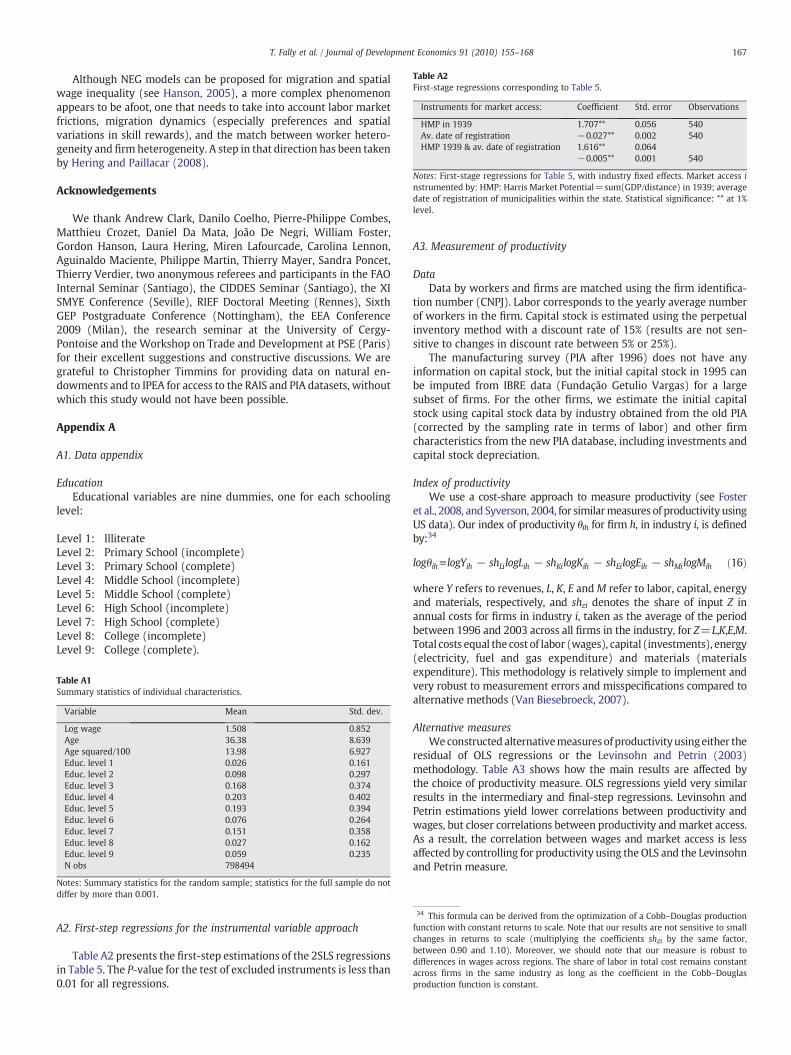
Table A2First-stage regressions corresponding to Table 5.

Instruments for market access: Coefficient Std. error Observations

HMP in 1939 1.707** 0.056 540Av. date of registration −0.027** 0.002 540HMP 1939 & av. date of registration 1.616** 0.064

−0.005** 0.001 540

Notes: First-stage regressions for Table 5, with industry fixed effects. Market access instrumented by: HMP: Harris Market Potential=sum(GDP/distance) in 1939; averagedate of registration of municipalities within the state. Statistical significance: ** at 1%level.


Although NEG models can be proposed for migration and spatialwage inequality (see Hanson, 2005), a more complex phenomenonappears to be afoot, one that needs to take into account labor marketfrictions, migration dynamics (especially preferences and spatialvariations in skill rewards), and the match between worker hetero-geneity and firm heterogeneity. A step in that direction has been takenby Hering and Paillacar (2008).

Acknowledgements

We thank Andrew Clark, Danilo Coelho, Pierre-Philippe Combes,Matthieu Crozet, Daniel Da Mata, João De Negri, William Foster,Gordon Hanson, Laura Hering, Miren Lafourcade, Carolina Lennon,Aguinaldo Maciente, Philippe Martin, Thierry Mayer, Sandra Poncet,Thierry Verdier, two anonymous referees and participants in the FAOInternal Seminar (Santiago), the CIDDES Seminar (Santiago), the XISMYE Conference (Seville), RIEF Doctoral Meeting (Rennes), SixthGEP Postgraduate Conference (Nottingham), the EEA Conference2009 (Milan), the research seminar at the University of Cergy-Pontoise and the Workshop on Trade and Development at PSE (Paris)for their excellent suggestions and constructive discussions. We aregrateful to Christopher Timmins for providing data on natural en-dowments and to IPEA for access to the RAIS and PIA datasets, withoutwhich this study would not have been possible.

Appendix A

A1. Data appendix

EducationEducational variables are nine dummies, one for each schooling

level:

Level 1: IlliterateLevel 2: Primary School (incomplete)Level 3: Primary School (complete)Level 4: Middle School (incomplete)Level 5: Middle School (complete)Level 6: High School (incomplete)Level 7: High School (complete)Level 8: College (incomplete)Level 9: College (complete).

34 This formula can be derived from the optimization of a Cobb–Douglas productionfunction with constant returns to scale. Note that our results are not sensitive to smallchanges in returns to scale (multiplying the coefficients shZi by the same factor,between 0.90 and 1.10). Moreover, we should note that our measure is robust todifferences in wages across regions. The share of labor in total cost remains constantacross firms in the same industry as long as the coefficient in the Cobb–Douglasproduction function is constant.

Table A1Summary statistics of individual characteristics.

Variable Mean Std. dev.

Log wage 1.508 0.852Age 36.38 8.639Age squared/100 13.98 6.927Educ. level 1 0.026 0.161Educ. level 2 0.098 0.297Educ. level 3 0.168 0.374Educ. level 4 0.203 0.402Educ. level 5 0.193 0.394Educ. level 6 0.076 0.264Educ. level 7 0.151 0.358Educ. level 8 0.027 0.162Educ. level 9 0.059 0.235N obs 798494

Notes: Summary statistics for the random sample; statistics for the full sample do not

A2. First-step regressions for the instrumental variable approach

Table A2 presents the first-step estimations of the 2SLS regressionsin Table 5. The P-value for the test of excluded instruments is less than0.01 for all regressions.

differ by more than 0.001.

A3. Measurement of productivity

DataData by workers and firms are matched using the firm identifica-

tion number (CNPJ). Labor corresponds to the yearly average numberof workers in the firm. Capital stock is estimated using the perpetualinventory method with a discount rate of 15% (results are not sen-sitive to changes in discount rate between 5% or 25%).

The manufacturing survey (PIA after 1996) does not have anyinformation on capital stock, but the initial capital stock in 1995 canbe imputed from IBRE data (Fundação Getulio Vargas) for a largesubset of firms. For the other firms, we estimate the initial capitalstock using capital stock data by industry obtained from the old PIA(corrected by the sampling rate in terms of labor) and other firmcharacteristics from the new PIA database, including investments andcapital stock depreciation.

Index of productivityWe use a cost-share approach to measure productivity (see Foster

et al., 2008, and Syverson, 2004, for similarmeasures of productivity usingUS data). Our index of productivity θih for firm h, in industry i, is definedby:34

logθihulogYih − shLilogLih − shKilogKih − shEilogEih − shMilogMih ð16Þ

where Y refers to revenues, L, K, E andM refer to labor, capital, energyand materials, respectively, and shzi denotes the share of input Z inannual costs for firms in industry i, taken as the average of the periodbetween 1996 and 2003 across all firms in the industry, for Z=L,K,E,M.Total costs equal the cost of labor (wages), capital (investments), energy(electricity, fuel and gas expenditure) and materials (materialsexpenditure). This methodology is relatively simple to implement andvery robust to measurement errors and misspecifications compared toalternative methods (Van Biesebroeck, 2007).

Alternative measuresWeconstructed alternativemeasuresofproductivityusingeither the

residual of OLS regressions or the Levinsohn and Petrin (2003)methodology. Table A3 shows how the main results are affected bythe choice of productivity measure. OLS regressions yield very similarresults in the intermediary and final-step regressions. Levinsohn andPetrin estimations yield lower correlations between productivity andwages, but closer correlations between productivity and market access.As a result, the correlation between wages and market access is lessaffected by controlling for productivity using the OLS and the Levinsohnand Petrin measure.

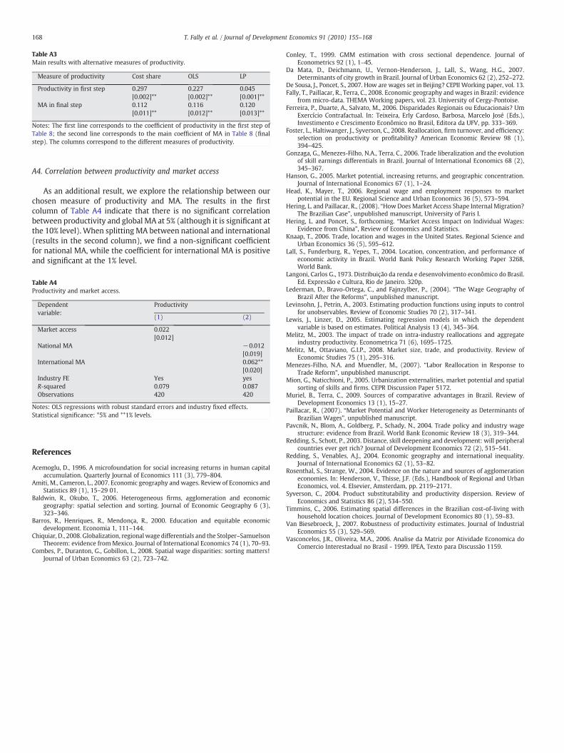
Table A3Main results with alternative measures of productivity.

Measure of productivity Cost share OLS LP

Productivity in first step 0.297 0.227 0.045[0.002]** [0.002]** [0.001]**

MA in final step 0.112 0.116 0.120[0.011]** [0.012]** [0.013]**

Notes: The first line corresponds to the coefficient of productivity in the first step ofTable 8; the second line corresponds to the main coefficient of MA in Table 8 (final


A4. Correlation between productivity and market access

As an additional result, we explore the relationship between ourchosen measure of productivity and MA. The results in the firstcolumn of Table A4 indicate that there is no significant correlationbetween productivity and global MA at 5% (although it is significant atthe 10% level). When splitting MA between national and international(results in the second column), we find a non-significant coefficientfor national MA, while the coefficient for international MA is positiveand significant at the 1% level.

step). The columns correspond to the different measures of productivity.

Table A4Productivity and market access.

Dependentvariable:

Productivity

(1) (2)

Market access 0.022[0.012]

National MA −0.012[0.019]

International MA 0.062**[0.020]

Industry FE Yes yesR-squared 0.079 0.087Observations 420 420

Notes: OLS regressions with robust standard errors and industry fixed effects.Statistical significance: *5% and **1% levels.

References

Acemoglu, D., 1996. A microfoundation for social increasing returns in human capitalaccumulation. Quarterly Journal of Economics 111 (3), 779–804.

Amiti, M., Cameron, L., 2007. Economic geography andwages. Review of Economics andStatistics 89 (1), 15–29 01.

Baldwin, R., Okubo, T., 2006. Heterogeneous firms, agglomeration and economicgeography: spatial selection and sorting. Journal of Economic Geography 6 (3),323–346.

Barros, R., Henriques, R., Mendonça, R., 2000. Education and equitable economicdevelopment. Economia 1, 111–144.

Chiquiar, D., 2008. Globalization, regionalwage differentials and the Stolper–SamuelsonTheorem: evidence fromMexico. Journal of International Economics 74 (1), 70–93.

Combes, P., Duranton, G., Gobillon, L., 2008. Spatial wage disparities: sorting matters!Journal of Urban Economics 63 (2), 723–742.

Conley, T., 1999. GMM estimation with cross sectional dependence. Journal ofEconometrics 92 (1), 1–45.

Da Mata, D., Deichmann, U., Vernon-Henderson, J., Lall, S., Wang, H.G., 2007.Determinants of city growth in Brazil. Journal of Urban Economics 62 (2), 252–272.

De Sousa, J., Poncet, S., 2007. How are wages set in Beijing? CEPII Working paper, vol. 13.Fally, T., Paillacar, R., Terra, C., 2008. Economic geography and wages in Brazil: evidence

from micro-data. THEMA Working papers, vol. 23. University of Cergy-Pontoise.Ferreira, P., Duarte, A., Salvato, M., 2006. Disparidades Regionais ou Educacionais? Um

Exercício Contrafactual. In: Teixeira, Erly Cardoso, Barbosa, Marcelo José (Eds.),Investimento e Crescimento Econômico no Brasil, Editora da UFV, pp. 333–369.

Foster, L., Haltiwanger, J., Syverson, C., 2008. Reallocation, firm turnover, and efficiency:selection on productivity or profitability? American Economic Review 98 (1),394–425.

Gonzaga, G., Menezes-Filho, N.A., Terra, C., 2006. Trade liberalization and the evolutionof skill earnings differentials in Brazil. Journal of International Economics 68 (2),345–367.

Hanson, G., 2005. Market potential, increasing returns, and geographic concentration.Journal of International Economics 67 (1), 1–24.

Head, K., Mayer, T., 2006. Regional wage and employment responses to marketpotential in the EU. Regional Science and Urban Economics 36 (5), 573–594.

Hering, L. and Paillacar, R., (2008). “HowDoes Market Access Shape Internal Migration?The Brazilian Case”, unpublished manuscript, University of Paris I.

Hering, L. and Poncet, S., forthcoming. “Market Access Impact on Individual Wages:Evidence from China”, Review of Economics and Statistics.

Knaap, T., 2006. Trade, location and wages in the United States. Regional Science andUrban Economics 36 (5), 595–612.

Lall, S., Funderburg, R., Yepes, T., 2004. Location, concentration, and performance ofeconomic activity in Brazil. World Bank Policy Research Working Paper 3268,World Bank.

Langoni, Carlos G., 1973. Distribuição da renda e desenvolvimento econômico do Brasil.Ed. Expressão e Cultura, Rio de Janeiro. 320p.

Lederman, D., Bravo-Ortega, C., and Fajnzylber, P., (2004). “The Wage Geography ofBrazil After the Reforms”, unpublished manuscript.

Levinsohn, J., Petrin, A., 2003. Estimating production functions using inputs to controlfor unobservables. Review of Economic Studies 70 (2), 317–341.

Lewis, J., Linzer, D., 2005. Estimating regression models in which the dependentvariable is based on estimates. Political Analysis 13 (4), 345–364.

Melitz, M., 2003. The impact of trade on intra-industry reallocations and aggregateindustry productivity. Econometrica 71 (6), 1695–1725.

Melitz, M., Ottaviano, G.I.P., 2008. Market size, trade, and productivity. Review ofEconomic Studies 75 (1), 295–316.

Menezes-Filho, N.A. and Muendler, M., (2007). “Labor Reallocation in Response toTrade Reform”, unpublished manuscript.

Mion, G., Naticchioni, P., 2005. Urbanization externalities, market potential and spatialsorting of skills and firms. CEPR Discussion Paper 5172.

Muriel, B., Terra, C., 2009. Sources of comparative advantages in Brazil. Review ofDevelopment Economics 13 (1), 15–27.

Paillacar, R., (2007). “Market Potential and Worker Heterogeneity as Determinants ofBrazilian Wages”, unpublished manuscript.

Pavcnik, N., Blom, A., Goldberg, P., Schady, N., 2004. Trade policy and industry wagestructure: evidence from Brazil. World Bank Economic Review 18 (3), 319–344.

Redding, S., Schott, P., 2003. Distance, skill deepening and development: will peripheralcountries ever get rich? Journal of Development Economics 72 (2), 515–541.

Redding, S., Venables, A.J., 2004. Economic geography and international inequality.Journal of International Economics 62 (1), 53–82.

Rosenthal, S., Strange, W., 2004. Evidence on the nature and sources of agglomerationeconomies. In: Henderson, V., Thisse, J.F. (Eds.), Handbook of Regional and UrbanEconomics, vol. 4. Elsevier, Amsterdam, pp. 2119–2171.

Syverson, C., 2004. Product substitutability and productivity dispersion. Review ofEconomics and Statistics 86 (2), 534–550.

Timmins, C., 2006. Estimating spatial differences in the Brazilian cost-of-living withhousehold location choices. Journal of Development Economics 80 (1), 59–83.

Van Biesebroeck, J., 2007. Robustness of productivity estimates. Journal of IndustrialEconomics 55 (3), 529–569.

Vasconcelos, J.R., Oliveira, M.A., 2006. Analise da Matriz por Atividade Economica doComercio Interestadual no Brasil - 1999. IPEA, Texto para Discussão 1159.

Economic geography and wages in Brazil: Evidence...

Documents

Transcript of Economic geography and wages in Brazil: Evidence...