- 1-

Economic Analysis in Support of Bilateral and Multilateral Trade Negotiations

ECONOMIC IMPACT

OF POTENTIAL OUTCOME OF THE DDA II

CEPII-CIREM

This report has been prepared by

Yvan Decreux and Lionel Fontagné

Research assistance: Emmanuel Milet

Final Report

October 2011

Disclaimer

This study benefited from the financial support of the European Commission DG Trade.

The views and opinions presented in this document do not necessarily reflect those of DG Trade or the European

Commission.

- 2-

Content

Executive summary ................................................................................................................................................. 3

1. Introduction ..................................................................................................................................................... 5

2. Why trade facilitation matters ......................................................................................................................... 8

Definition ............................................................................................................................................................ 8 Assessing the red tape costs ................................................................................................................................ 9 The potential benefits of trade facilitation .......................................................................................................... 9 Methods for assessing trade facilitation effects................................................................................................. 11

3. Sources and modelling assumptions ............................................................................................................. 13

Draft modalities ................................................................................................................................................. 13 The MIRAGE model ......................................................................................................................................... 14 GTAP and protection data ................................................................................................................................. 15 Baseline and modelling of the shocks ............................................................................................................... 15 The different scenarios ...................................................................................................................................... 19

4. Details of the scenarios concerning trade in agricultural goods .................................................................... 21

5. Modalities for the NAMA ............................................................................................................................. 25

6. Overall results of the central scenario ........................................................................................................... 27

7. Sectoral impact of the central scenario.......................................................................................................... 33

8. Detailed impacts on factor incomes of the central scenario .......................................................................... 37

9. Sectoral initiatives ......................................................................................................................................... 42

10. How do these results compare with the related literature? ............................................................................ 46

11. Conclusion .................................................................................................................................................... 49

12. References ..................................................................................................................................................... 50

13. Appendix ....................................................................................................................................................... 54

- 3-

Executive summary

The current Round of multilateral negotiations that took was launched in Doha in November 2001

has reached a critical point. Following a Ministerial meeting in July 2008 that came close to

reaching agreement on modalities for non-agricultural market access (NAMA) and agriculture,

work has continued in Geneva, but the whole process looked to be at risk in mid-2011. In April

2011, the negotiations on NAMA encountered the stumbling block of sectoral initiatives. By June

2011, it was clear that completion of a comprehensive agreement on all topics was impossible by

the end of this year, but it was hoped that agreement could be reached on an “LDC plus” including

trade facilitation. Currently, this looks to be in doubt as well, and the 8th WTO Ministerial

Conference in December 2011 is expected to discuss a more productive way forward in the

negotiations.

In this report, we tentatively address the economic impact of a deal integrating the most recent

proposals circulated in the multilateral trade negotiations arena, especially sectorals in NAMA, in

order to shed some light on the gains that a successful outcome would imply, including as regards

an agreement on trade facilitation.

The sources used to assess the consequences of the negotiations are highly technical and complex,

reflecting the difficulties involved for negotiators to find a politically acceptable deal (e.g.

exceptions as well as compensatory import commitments, such as tariff rate quotas, are

introduced). The consequences of an agreement, involving cuts that differ by country and by

product, cannot be assessed without recourse to quantitative and detailed representation of the

world economy. This report tries to assess the impact of the proposals on the world economy. We

measure border protection at the most detailed level possible (product, importer, exporter), and

through computation of the liberalisation resulting from a tariff-cutting formula. Bound and

applied duties (ad valorem, specific, mixed or compound) are measured at the Harmonised System

6-digit (HS-6) product level (the most disaggregated level for which we have harmonised

information).

The data are from the Global Trade Analysis Project (GTAP) and Market Access Map (MAcMap),

and describe the 2004 economy. We run a “pre-experiment” introducing the accumulated changes

affecting the world economy in the period 2004 to 2010. In 2012 (and subsequent years depending

on the timing of phasing out of the protection) the scenarios described below will be implemented.

Phasing out is applied linearly over a five-year period for developed countries (10 years for

developing countries). Recently acceded countries will be granted respectively longer periods, here

we make the simplifying assumption that these countries will have 12 years for phasing out of

protection. Finally, we compare situations for the world economy between 2013 and 2025, with

- 4-

and without liberalisation. The Least Developed Countries (LDCs) will not be asked to reduce

their tariffs, only to increase binding coverage.

The first scenario depicts the joint effect of modalities for agriculture and NAMA. The three

pillars of agriculture are introduced. NAMA data are based on the coefficients for the Swiss

formula as contained in the 2008 draft modalities text. The second scenario adds a 3% reduction

to protection for trade in services. The third scenario should be considered the core scenario in

this exercise: it combines liberalisation of trade in goods and services with a rather ambitious trade

facilitation scenario. The remaining four scenarios are systematically benchmarked against this

central scenario. The fourth scenario adds improved port efficiency; the fifth scenario adds

sectoral initiatives for chemicals, electronic products and machinery; the sixth adds a duty free

initiative for environmental goods;1 the final, the seventh scenario is a ‘softer’ version of scenario

six: tariffs are applied to environmental goods according to a more aggressive Swiss formula

(smaller coefficient) than for other NAMA goods, as opposed to zero tariffs in scenario six.

We observe a $US70bn world Gross Domestic Product (GDP) long run gain when agriculture and

industry are liberalised, a $US85bn gain when a 3% reduction in protection for services is added to

certain services sectors. Calculation of the gains associated with trade facilitation suggests roughly

a doubling of the expected gains ($US152bn); port efficiency adds another $US35bn.

In total, the $US187bn gains identified here in the scenario combining liberalisation in trade in

goods and services with trade facilitation and port efficiency, would accumulate to world GDP

every year in the medium term, compared to the situation without agreement. Recent proposals for

sectoral initiatives would add a further $US15bn on top of these gains.

Interestingly, in value terms the European Union (EU) would reap the second largest increase in

industrial exports, just after China, and the highest increase for its exports of services. Other

emerging economies and the USA would benefit from an ambitious conclusion to the Round,

although US gains appear rather limited when expressed as percentage of GDP.

1We use the WTO list of environmental products. See Committee on Trade and Environment Special Session, 21

April 2011.

- 5-

1. Introduction

The multilateral negotiations launched in Doha in November 2001 have reached a critical point.

On 19 May 2008, Crawford Falconer, Chairman of the agriculture negotiations, circulated revised

draft modalities, and on the same day Don Stephenson released the revised draft negotiating text

for Non-Agricultural Market Access (NAMA). However, ministerial level agreement and

consensus on associated fine tuning of the proposals were not achieved. On 12 December 2008,

the Secretary General of the World Trade Organization (WTO) decided there would be no

ministerial level meeting that month. Work continued in Geneva, but in mid 2011 the whole

process looks to be very much at risk. In April 2011 the negotiating group on NAMA was

confronted by the seemingly irresolvable problem of sectoral initiatives. Following the collapse in

world trade, there was renewed interest in re-visiting the Doha Development Agenda (DDA) deal.

However, the political willingness to conclude negotiations seemed very uncertain, possibly due to

the world financial crisis. On 29 March 2011, the Director General of the WTO declared that “[it

is] time (…), to reflect on the consequences of failure” stating that “The absence of progress in

NAMA sectorals constitutes today a major obstacle to progress on to the remaining market access

issues”. By June 2011, it was clear that completion of a comprehensive agreement on all topics

was impossible by the end of this year, but it was hoped that agreement could be reached on an

“LDC plus” including trade facilitation. On 22 June 2011 the Director General of the WTO

suggested focusing on a “December [2011] Ministerial package on trade benefits for the poorest

countries”. On 24th June he reiterated this suggestion in Brussels at the World Customs

Organization, pointing to the gains to be achieved from facilitating trade for developing countries.

It is hoped that the December 2011 Ministerial meeting will reach a deal on this issue which is so

important for development and for keeping the Round alive. Discussion on other issues, such as

market access, could resume in 2012 (possibly after the US Presidential elections), based on the

modalities already discussed. Currently, this looks to be in doubt as well, and the 8th WTO

Ministerial Conference in December 2011 is expected to discuss a more productive way forward in

the negotiations.

In order to understand the reasons for the impasse, we conduct an exercise to examine the

economic impact of a deal integrating the most recent proposals circulated in the arena of the

multilateral trade negotiations, including sectorals in NAMA. This is an important exercise both

because the new proposals include even more precise prescriptions than in the 2008 draft and

because the context has undergone radical changes. The crisis has penalised certain regions of the

world to a greater extent, which has required a revision to growth prospects. New Free Trade

Areas (FTAs) have also been established. Finally, the emerging economies are reluctant to sign up

to the sectoral initiatives, which will have complex impacts when combined with the existing

- 6-

mechanisms to achieve flexibility. We try also to identify the extent of possible windows of

opportunity in terms of the gains to be expected from an agreement on trade facilitation.

In this context of possible, perhaps not very plausible, completion of the negotiations, it is

extremely important precisely to quantify the potential gains associated with the completion of the

Round and how these gains will be shared among countries.

Our exercise reveals impacts that cannot be compared directly with the orders of magnitude

associated with failure of the Round. In the case of failure, a resurgence of protectionism, either

within the strict boundaries of WTO rules (e.g. an increase in tariffs up to their bounds), at the

fringes of it (generalising contingent protection), or outside of it (unilateral increases in protection)

would have a cost corresponding to a multiple of the gains considered here (Bouët and Laborde,

2009).

We should point also to the nature of the gains considered here. In line with the mandate of

negotiators, we compute gains in exports. Steady progress has been made in the General

Agreement on Tariffs and Trade (GATT) arena through the adoption of a rather mercantilist

approach to market access: in order to have offensive interests endorsed by trade partners, the

focal country must open its own market. Indeed, from an analytical point of view, this outcome

leads to real economic gains due to a better allocation of resources, productivity gains and

additional income. In our economic analysis, we refer to income generally (or to value added or

Gross Domestic Product - GDP).

The documents for assessing the consequences of the negotiations are highly technical and

complex documentation, mirroring the degree of imagination among the negotiators to find a

politically acceptable deal. A very simple modality, such as use of a non-linear tariff cut formula

applied to every tariff line as opposed to negotiation product by product, is a very convenient

design. If properly calibrated, such a measure can have an aggressive effect on tariff peaks and,

accordingly, greatly reduce induced distortions. It simplifies negotiation over reciprocal

concessions among the large number of participating countries. However, exceptions arise in the

form of internal resistance among negotiating countries. The designation of exceptions, however,

must still follow certain rules (e.g. non-concentration clauses). Minimum or maximum average

cuts are added to the liberalisation scheme. Less strict treatment is proposed for small and

vulnerable economies; membership of a customs union implies specific treatments for some

members as well as a number of exceptions. Specific issues, such a tropical products or tariff

escalation, are addressed by modification to the general pattern of modalities. All these details are

taken into consideration in this report.

Ultimately, we have an intricate design: the consequences of such an agreement, leading to cuts

that differ by country and by product, certainly cannot be assessed without resorting to a

- 7-

quantitative and detailed representation of the world economy. This report provides an assessment

of the impact of these negotiating proposals on the world economy.

Section 2 explains why trade facilitation plays such a large role in our results. Section 3 presents

the modelling assumptions and Section 4 describes the agricultural negotiations in detail. Section 5

presents NAMA. The overall results of the negotiations are presented in Section 6. Section 7

discusses the impacts of the main scenario on three broad sectors and the impacts on factor

incomes are examined in detail in Section 8. The impact of sectoral initiatives compared to our

central scenario, is examined in Section 9. Section 10 compares our results with findings in the

literature and Section 11 provides some conclusions.

- 8-

2. Why trade facilitation matters

Trade facilitation in the Doha Round negotiations is often seen as an unexpected low-hanging

fruit, “as the seemingly win-win negotiations have moved steadily over the past few years, even as

other areas of the Doha talks have stalled” (a WTO official speaking in 2010).2

Transaction costs imposed on international trade have attracted the interest of empirical research

and policy making. Empirical evidence shows that poor-quality border management and logistics

have a negative effect on trade. For this reason the WTO initiated a process of trade facilitation

relying on “the simplification and the harmonization of trade procedures, i.e. activities, practices

and formalities related to the collection, the presentation, the communication and the treatment of

data required for the movement of goods in international trade” (WTO, 2002).

Definition

Trade facilitation can be defined as a process encompassing five main topics:

- simplification of trade procedures and documentation;

- harmonization of trade practices and rules;

- more transparent information and procedures for international flows;

- recourse to new technologies promoting international trade

- more secure modes of payment for international commerce (more reliable and faster).

These issues can be described as “non-official barriers” or “red-tape costs” because they are not

classified within an official framework that includes governments and organisations.

Most trade facilitation studies are legal or a descriptive (Messerlin and Zarrouk, 1999; Woo and

Wilson, 2000; Wilson et al., 2002; OECD, 2002c, OECD, 2002d, WTO, 2002; OECD, 2002c;

OECD, 2002d). They do not provide an empirical assessment of the effect of trade facilitation, but

examine its legal aspects by analysing Articles V, VIII and X of GATT (which we present later).

In this report, we build on the existing literature to provide a quantitative assessment of the impact

of trade facilitation in general equilibrium.

While trade liberalization refers to the reduction in the traditional barriers impeding international

trade, such as tariffs or quotas, trade facilitation incorporates the elements referred to above which

make trade easier, but will require specific adaptation to our modelling framework. Improving port

efficiency is often considered part of the trade facilitation process, but often requires huge

investment, beyond institutional or administrative adaptations. In what follows, and in our

modelling exercise, we treat port efficiency separately: it is more difficult to ascertain the gains

2 We are indebted to Chahir Zaki (PSE) for his advice on trade facilitation issues.

- 9-

from it, and the cost of implementing such as policy is also hard to evaluate. This makes us less

confident about the results obtained. Our central scenario, therefore, uses trade facilitation only.

We fist consider how to assess red tape costs that can be reduced through trade facilitation.

Assessing the red tape costs

Numerous methods can be applied to quantify red tape costs. Analytical studies generally examine

the level of these costs through cross-section comparison among many countries (OECD, 2002a;

OECD, 2002d). The cost of administrative barriers has been shown to account for 2%-15% of the

value of traded goods. OECD (2002b) argues that this large range can be explained by three

factors: differences in the reference year of the study, aspects of the administrative barriers

considered; and the sample of countries.

Surveys have also been used to provide qualitative analysis of the various costs associated with

each administrative barrier (Asia Pacific Economic Co-operation, 1999; Duval, 2006). They rely

on the opinions of experts and representatives of firms involved in international trade. They found

that it is the costs resulting from the complexity of customs regulations that is the greatest

obstacle: a majority of interviewees classified it as being a serious or very serious barrier.

Finally, the ad-valorem equivalent (AVE) technique has been used to determine the value of time

to transport (Minor and Tsigas, 2008; Hummels, 2001). Zaki (2009) shows that the AVEs of time

depend on both the level of development of the economy and the traded product. For instance,

Tanzania's average AVE of time to export and to import is 80%, while the US AVE is 1%. Also

garment AVEs are higher than tobacco AVEs because the former are more sensitive to time than

the latter.

Instead of introducing tariff equivalents of trade facilitation in our modelling, we adopt a different

and innovative strategy based on the cost of time to trade. We use a modified MIRAGE model in

order to incorporate trade costs that add up to ordinary freight costs. Data on trade costs are

provided by Minor and Tsigas (2008). Their measure of trade costs is based on the time necessary

to ship a good from one country to another, taken from the World Bank’s Doing Business reports.

The details of our modelling assumptions are explained in Section 3.

The potential benefits of trade facilitation

To remove red-tape costs, a country must bear the cost of implementing trade facilitation

measures. OECD (2003b) and Duval (2006) show that implementation involves six types of costs:

legislative, institutional, training, infrastructure, operational and political. As already mentioned,

we treat infrastructure, especially concerning ports, separately.

- 10-

Legislative costs are related to new regulations necessary to provide a sound legal framework for

trade facilitation. Institutional costs are linked to the establishment of new institutions (new

customs), new services (the single window) and new teams (the risk management teams). Training

costs are associated with training existing staff in new software, computerized customs, etc.

Financial aid or trade aid might help developing countries to defray these unavoidable costs.

Operational costs are associated with the maintenance of trade facilitation measures (Duval, 2006).

The amount of time (and therefore costs) involved is not trivial in relation to items such as

updating software and upgrading computer machinery in existing customs authorities (Roy and

Bagai, 2005). The last type of cost, political costs, has two facets. On the one hand, existing staff

may be opposed to the introduction of a new system seeing the existing one as still generating

rents. On the other hand, policy makers may be more or less keen to pursue implementation of the

reforms (Duval, 2006).

Nevertheless, the benefits of trade facilitation have been shown to be more important than its

underlying costs. Zaki (2010) runs a simulation for the Egyptian economy to assess the benefits of

trade facilitation, obtaining net positive effects for the whole economy. The process is shown to

increase public sector efficiency and enable government to cut redundant resources.

It should be noted, however, that these benefits vary at different levels and developing countries

gain more than developed ones. The Organisation for Economic Cooperation and Development

(OECD) has carried out many studies which show that developing countries gain two-thirds of the

full benefits of trade facilitation (OECD, 2003b). Similarly, Francois et al. (2005) find that the

developing countries gains from trade facilitation are higher than the share of developed ones.

Wilson, Mann and Otsuki (2004) posit very large GDP per capita gains for certain developing

countries and forecast that trade flows should increase by 40.3% for South Asia, 30% for Central

and Eastern European countries, 24% for East Asia and 20% for the Caribbean and Latin America

against 4% for the OECD countries (Wilson et al., 2004). These figures reveal that developing

countries where trade procedures are especially cumbersome and outdated, should gain more from

trade facilitation than developed economies.

At the product level, trade in perishable (e.g. vegetables), seasonal (e.g. textiles and garments),

high value-added commodities (high-technology products with a short market-lifetime) is boosted

because these goods are time-sensitive.

Finally, at the firm level, small and medium sized enterprises (SMEs) benefit more and their gains

are important since SME incur much higher costs than multinationals. The costs for SMEs from

developing countries are made higher by the fact that they do not have good historical experience

with with the customs authorities in the richer countries. They are also seen as high-risk firms and

flows involving developed economies are subject to numerous physical checks and more complex

- 11-

documentation. To increase the benefits to SMEs, the effects of trade facilitation measures must be

the same for large firms and SMEs.

Methods for assessing trade facilitation effects

Empirical studies investigating the effect of trade facilitation on trade and welfare use mainly one

of two methodologies: gravity models or Computable General Equilibrium (CGE) models.

Gravity models are appropriate for measuring the impact of aspects of trade facilitation on trade.

They have become an essential tool for measuring the impact of tariff and non-tariff barriers on the

flow of goods and services (Anderson, 1979; Bergstrand, 1989, 1990; Baier and Bergstrand,

2001). The literature on trade facilitation and gravity models falls into three main categories. The

first includes studies that emerged in the wake of McCallum's (1995) work which uses models to

quantify border effects. However, trade facilitation is not explicitly included since it is introduced

either in terms of the border effect term or other border related costs. The second encompasses

models that treat just one aspect of trade facilitation, referred to as “mono-dimensional models”.

For instance, Freund and Weinhold (2000) examine the impact of the internet on trade, Hummels

(2001) and Djankov et al. (2006) examine the impact of time, Limao and Venables (2000) the

impact of efficient infrastructure and Dutt and Traca (2007) study the effect of corruption on trade.

Third are the models that incorporate several aspects of trade facilitation, or “multi-dimensional

models”. Wilson, Mann and Otsuki (2003 and 2004) and Kim et al. (2004), did some pioneering

work on multi-dimensional models, quantifying the impact of trade facilitation measures using a

gravity model that takes account of port efficiency, e-business intensity, and the regulatory and

customs environments. They apply this model to the Asia-Pacific Economic Cooperation (APEC)

countries and then extend it to a larger sample of countries.

CGE models are the second tool used to assess the welfare effect of trade facilitation on either a

particular economy using a monocountry model, or on the whole world using a multinational

models. We use the CGE model MIRAGE for the analysis in this report. Hertel et al. (2001) was

one of the first studies to use a modified Global Trade Analysis Project (GTAP) model to analyse

the Japan-Singapore free trade agreement, introducing time costs as a technical shift in the

Armington import demand function. Fox et al. (2003) also use the GTAP model, but introduce an

import-augmenting technical change which allowed them to simulate the removal of an iceberg

tariff by applying a positive shock to the technical efficiency of the trade flow. APEC (1999)

models trade facilitation, using the GTAP model; it shows an increase in the productivity of the

international transportation sector to capture the downward shift in the supply line of imports

resulting from the implementation of cost-reducing measures.

- 12-

Francois et al. (2003, 2005) show that trade facilitation explains one-third of the gains in

productivity showing that these barriers are a “pure deadweight loss”, for Asia-Pacific developing

countries. Dennis (2006) shows that welfare gains could triple if regional trade agreements

between some Mediterranean countries and the European Union are complemented by improved

trade facilitation. Along the same lines, Hoekman and Konan (1999) assess the impact of a deep

integration between Egypt and the European Union (EU). They show that a shallow agreement

(elimination of Egyptian tariffs) with the EU can lead to a welfare decline. Meanwhile, if deep

integration efforts are pursued by eliminating regulatory barriers and red-tape costs, welfare gains

may increase significantly.

Zaki (2010) adopts a two-tier approach, combining a gravity and a CGE model. In a first step, Zaki

(2009) uses a gravity model to estimate the AVEs of administrative barriers. First, the transaction

time to import and export is estimated, which sheds light on some important determinants of

transaction time: documents (capturing the impact of time-increasing bureaucracy), the internet (as

a proxy for technological intensity which reduces time), geographic variables (such as being

landlocked, which hinders trade), corruption (as a proxy for customs fraud) and the number of

procedures involved in setting up a business (which is an indication of the efficiency of the

institutional environment). The predicted time to trade is introduced in the gravity model to

determine its effect on bilateral trade. Adopting Kee et al.’s (2008) methodology to estimate the

AVEs of non-tariff barriers, the gravity model outcome can be used to compute the AVEs of the

administrative barriers to trade and show that the internet, bureaucracy, corruption and geographic

variables significantly affect the transaction time to trade. If sectoral characteristics are taken into

account, perishable (food and beverages), seasonal (apparel) and high-value added products appear

to be more sensitive to transaction time than other products. The AVEs of these goods are much

higher than the AVE for other manufactured goods.

In a second step the estimated AVEs are introduced into the MIRAGE model in the form of an

iceberg cost. Two simulations are performed. First, partial removal of the administrative barriers is

simulated by reducing the trade cost for all countries by 50%. Second, in order to compare trade

facilitation and trade liberalization effects, a similar shock is applied to tariffs. This exercise

confirms that developing countries in Africa and Asia, especially Sub-Saharan Africa, the Middle

East and North Africa, gain much more than developed countries and the process enables

important export diversification. At the sectoral level, food, textiles and electronics benefit more

than other products. Lastly, the impact of trade facilitation is shown to be large compared to tariff

reductions.

- 13-

3. Sources and modelling assumptions

The intricate nature of the proposals discussed by negotiators, which include numerous exceptions

to a series of rules applied at product level, imposes a specific modelling strategy. The state of the

art is measurement of border protection at the most detailed level possible (product, importer,

exporter), and computation of liberalisation resulting from a tariff-cutting formula. Bound and

applied duties (whether ad valorem, specific, mixed or compound) need to be measured at the HS-

6 product level (the most disaggregated level for which harmonised information is available).

Draft modalities

The “Fourth revision of draft modalities for Non-Agricultural Market Access” published

December 2008, updated 21 April 2011, and including updated information on the actual

percentage to be applied to different modalities (e.g. 20% rather than x%), and information

collected on the option chosen by the main negotiating developing countries are the sources

informing our scenarios scenarios for the negotiation on non-agricultural goods (or NAMA).3

Sectoral initiatives concerning chemicals, machinery and electronic products and especially

environmental products have increased as a result of pressure from the developed countries. We

take these sectoral initiatives into account in additional simulations. Finally, we examine a less

strict version of the environmental simulation, in which tariffs on products identified as

environmental are not removed, but are replaced by the application of a more demanding Swiss

formula.

The sources of our data on agricultural goods include draft modalities and the report of the

Chairman of the Trade Negotiations Committee dated 21st April 2011.

4 We rely on the HS6 tariffs.

As exceptions are defined at the tariff line level, it allows more efficient use of flexibilities. This

affects the proposals, which allow an additional 2% of HS6 products to be classed as sensitive for

countries where protection is defined at the HS6 level. This is in line with previous estimations

based on a list of selected products in the EU from the 2,200 Combined Nomenclature 8-digit

(CN8) agricultural codes (out of 677 HS6 positions). We add this 2% to all countries that were

conceded sensitive products in agriculture. First, each tariff reduction scenario is quantified at

country, product and year level before being aggregated with the GTAP classification and

introduced in a CGE model for the global economy. In the context of agriculture, tariff rate quotas

(TRQs) are important. Reduced tariffs apply to many lines within quotas (inside tariff), with the

outside tariff providing greater protection. This is related to the selection of exceptions. When

3WTO, Negotiating Group on Market Access, document # TN/MA/W/103/Rev.3. The update is published as

“textual report by the chairman Ambassador LuziusWasescha, on the state of play in the NAMA negotiations”, 4 See WTO, Negotiating Group on Agriculture, documents, WTO, Negotiating Group on Agriculture, document

# TN/AG/26.

- 14-

agriculture tariff lines are classed as sensitive, an additional tariff quota must be opened.5

Industrial countries have the possibility of limiting the tariff cut to two-thirds of what it would be

based on the simple use of tiered formulas, and of compensating for this by a small quota.

Alternatively, they can choose to halve the cut and open a larger quota or keep only one third of

the cut and open a large quota. Modelling quotas should be done at the HS6-level, but this is very

demanding in terms of computing resources. In order to avoid explicitly modelling quotas, we use

the outside tariff under the assumption that the quota will quickly be filled as a result of growth in

world demand. Given the time horizon considered in our exercise, for most sectors this will be the

case. We assume also that countries choose the last option (a one-third cut). The likely impact of

this modelling assumption is underestimation of the impact of the DDA on EU agriculture in the

short run, in particular sectors with relatively high tariff protection, such as meat, ethanol, butter

and sugar. For this reason, we do not discuss short run changes; we consider only the long term

horizon where this assumption has very little effect.

The MIRAGE model

In the MIRAGE model the demand side is modelled for each region through a representative

agent. Domestic products are assumed to benefit from a specific status for consumers, making

them less substitutable by foreign products than foreign products among each other. Also,

manufactured products originating in developing and developed countries are assumed to belong

to different (price or) quality ranges. Hence, the competition among different quality products is

less tough than that between products of similar quality. To model the supply side, producers use

five factors: capital, labour (skilled and unskilled), land, and natural resources. The structure of

value-added is intended to take account of the well-documented skill-capital relative

complementarity. The production function assumes perfect complementarity between value-added

and intermediate consumption. The sectoral composition of the intermediate consumption

aggregate stems from a nested Constant Elasticity of Substitution (CES) function. For each sector

of origin, the sector bundle determining the origin of products has the same structure for final and

intermediate consumption.

In agricultural sectors, we assume constant returns to scale and perfect competition; in industry

and service sectors firms are assumed to face increasing returns to scale and imperfect

competition. In relation to market clearing and macroeconomic closure, capital goods are

accumulated every year as a result of investments in the most profitable sectors, but capital cannot

5 Since tariff rate quotas are not considered an optimal policy instrument, there have been requests for the

opening of new TRQs to be limited. Several options were considered; we adopted the intermediate suggestion

proposed at a special session of the Committee on Agriculture (6 December 2008, TN/AG/W/6) that the opening

of new TRQs should be limited to a maximum of 1% of agricultural tariff lines.

- 15-

change its sector allocation once installed. Natural resources are considered to be perfectly

immobile and not cumulative, both types of labour are assumed to be perfectly mobile across

sectors, and imperfect land mobility is modelled by a constant elasticity of transformation

function. Production factors are assumed to be fully employed; thus, negative shocks are absorbed

by changes in prices (factor rewards) rather than in quantities. All production factors are immobile

internationally. With respect to macroeconomic closure, the current balance is assumed to be

exogenous (and equal to its initial value in proportion to world GDP), while real exchange rates

are endogenous.

GTAP and protection data

MIRAGE relies on GTAP-8 data6 for 2004. This version of the database is preferred to the 2007

pre-release: the latter contains GDP projections that are already present in the dynamic baseline of

MIRAGE, while at the time of the present analysis, trade data had not been updated with actual

data. For internal consistency we use our own projections and rely on the trade matrices generated

by our model for the period 2004-2007. Tariff data on goods comes from Market Access Map

(MAcMap), version HS6-V3, hence, the most granular level of international trade classification of

products common to all countries refers to 2004. Further information on the construction of these

data, especially ad valorem equivalents, is provided in Bouët et al. (2008). Tariff equivalents of

services barriers previously were mainly based on Park (2002). We use here recent estimates by

CEPII (Fontagné et al., 2011).

Protection in services can take two forms. In communication and transport, we assume that it

consists of a barrier allowing the selected companies to increase their profit margins to their own

benefit. It is modelled as an export tax, thus mostly benefiting the exporting country. In other

services it is assumed to be cost-increasing, and is modelled as implying an additional iceberg

trade cost. In other words, this cost implies an additional use of all inputs (intermediate

consumption and factors) is needed to deliver the service to its final user.

Baseline and modelling of the shocks

The data available in GTAP and in MAcMap describe the 2004 economy. However, we know how

the world economy has behaved over the period 2004-2010. The model can be constrained to

comply with these macroeconomic observed developments. Accordingly, we run a “pre-

experiment” introducing the changes accruing to the world economy between 2004 and 2010. In

2012 (and subsequent years, depending on the timing of phasing out of protection), each of the

6 See https://www.gtap.agecon.purdue.edu/ for more details.

- 16-

scenarios described below is implemented. We then compare the situation of the world economy in

2013…2025, with and without this liberalisation. The reference situation over the whole period is

defined by the trajectory of the world economy up to 2013 forecast by the International Monetary

Fund (IMF), and from 2013 onwards as forecast by CEPII using a three-factor (labour, capital,

energy) growth model (Fouré et al., 2010).7 In this model, total population and labour force are

from the usual sources (International Labour Organization – ILO and United Nations – UN),

human capital formation is forecast on the basis of a catching up process, investment relies on

savings, savings are derived from a life cycle assumption, and total factor productivity (TFP) and

energy efficiency are also forecast.

Population and GDP are imposed on MIRAGE for every country or region and TFP is

endogenously adjusting at country level in the pre-experiment, with no difference between sectors.

Lastly, we perform simulations of the various shocks using these TFP changes as exogenous

variables; the oil (and primary resources) price is endogenous in the model and 2004 resources are

kept constant. Thus, the oil price is multiplied by 2.2 compared to world GDP price for 2004-2025

in the reference scenario.

Trade barriers are calculated on the 2004 picture of the world economy which takes account of the

Indian reform, augmented by the EU-Korea trade agreement.

Note that harmonised tariff data across countries is available at the HS6 level. In a global CGE

model such as MIRAGE, it is necessary to rely on information at this degree of detail, and for

every country in the world vis-à-vis each of their partners. Nevertheless, even this level of detail is

an approximation of actual negotiations at the tariff line level. In our exercise, tariffs are averaged

across tariff lines within HS6 positions. This inevitably leads to underestimation of the impact of

any tariff cut at the tariff line level. Partial equilibrium approaches possibly rely on more detailed

data, but they miss an explicit modelling of general equilibrium feed-backs.

For the NAMA as well as for agriculture, we model yearly tariff cuts at the product (HS6) and

country levels, before aggregation into the regional and sectoral decompositions of the model (see

Appendix 1). This takes account of the difference between bound and applied tariffs. In addition,

we model the reduction in internal support for agricultural products and the phasing out of export

subsidies. Lastly, because we lack precise information on potential liberalisation in services and

given the lack of ambition of negotiators in this field, we assume a 3% reduction in protection,

limited to all industrialised, most Latin American countries, and Asia except Central Asia. We

introduce flexibilities for special and sensitive products; we exempt the LDCs from tariff

reductions, consolidate the unbound tariffs, and take account of all additional elements contained

in the most recent Draft Modalities (see next section). Sectoral initiatives are modelled, starting

7 Centre d’Etudes Prospectives et d’Informations Internationales (CEPII).

- 17-

with chemical products. The reference agreement is the Chemical Tariff Harmonisation

Agreement (CTHA), which provides for a reduction in chemicals tariffs to 0%, 5.5% or 6.5% for

HS Chapters 28 to 39. The products include inorganic and organic chemicals, fertilisers and plant

protection chemicals, soaps and cosmetics, other chemicals and plastics. The 1995 agreement is

plurilateral.8 Next is machinery and then electronics. In these two sectors, the more ambitious

option is to set the bound tariffs to zero. The EU position is more accommodating than the US and

stresses that developing countries should be granted some flexibility even for sectorals.9 We adopt

the European approach. Also there is a published list of environmental goods for which tariffs

could be set to 0; we propose a phasing out of the corresponding tariffs in two simulations, based

on this list.

An important issue in the Round is trade facilitation. Although not at the forefront of negotiations,

progress on trade facilitation is crucial for developing economies, as we show below. In order to

measure the gains that would accrue from the implementation of a trade facilitation programme,

we propose a modified MIRAGE model to incorporate trade costs that add up to the ordinary

freight costs already present in the model. Data on trade costs are from Minor and Tsigas (2008),

based on work for the United States Agency for International development (USAID).10

Their

measure of trade costs is based on the time necessary to ship a good from a country to another, as

provided by the World Bank Doing Business reports. Transaction time is divided between time to

export and time to import. Within each of these categories, a distinction is made between inland

transportation from/to the port, customs procedure time, and time at the port to process the good

into/out of the ship. In the World Bank database, time does not depend on the good, but goods are

differentiated because the cost of time depends on the product. Minor and Tsigas provide a

measure of the daily cost of time as a percentage of the value of the good. The cost of time is

evaluated based on the preference for air or sea transport. Data are computed at the detailed level

and then aggregated to the GTAP aggregation level weighted by trade.

While we use the daily cost provided by Minor and Tsigas, we update the data on time using the

latest available data from the Doing Business website. In our experiment, only time at the frontier

(customs procedures and time at the port) is reduced. Transportation time to/from the port can vary

widely due to the different country sizes, but no improvement has been assumed for this trade cost.

8 Armenia, Australia, Bulgaria, Canada, Chile, Ecuador, EU, Hong Kong, Iceland, Japan, Jordan, Kirgizstan,

Republic of Korea, Mongolia, New Zealand , Norway, Oman, Panama, China, Qatar, Singapore, Switzerland,

Taiwan, Turkey, United Arab Emirates and the United States. 9 See EU statement at the TNC, 29 April 2011. This compromise would be threefold. Developed countries

eliminate tariffs for all products; developing countries eliminate tariffs for some products and reduce the end-

rates generated by the Swiss formula by a further fixed percentage point; in chemicals all developing countries

reduce their tariffs to at least the levels of the CTHA-tariff if it is lower than the result of the former rule. 10

USAID 2007. “Calculating Tariff Equivalents for Time in Trade”, March, downloadable from:

http://bizclir.com/cs/calculating_tariff_equivalents_for_time_in_trade

http://www.nathaninc.com/?downloadid=208

- 18-

Our trade facilitation experiment consists of dividing by two the processing time exceeding the

median level, for each category of trade costs (customs and port).11

Only members of the WTO

engage in the process. In a broader perspective, we consider another experiment where we add an

improvement to port efficiency.

After computing the costs before and after trade facilitation at the GTAP level, this information is

aggregated using trade as the weights, to match the aggregation level of the study.

In the simulation, we assume that trade facilitation can be achieved at no cost, although countries

may incur some costs to implement it, for example, the need to purchase modern equipment to

process goods at the ports and to cope with customs procedures. Trade facilitation can also

generate a cost by diverting qualified people from other productive sectors. These costs are not

incorporated in the model because of the absence of data. However, the gains implied by a rather

moderate scenario are quite significant and, thus, likely to outweigh any costs within a short period

of time.12

Since industrialised countries also benefit from trade facilitation, they may contribute to

the upgrading of developing countries’ infrastructures through the “aid for trade” scheme.

Also, since the EU-Korea agreement has been signed, we model this explicitly in the baseline

scenario. This reduces the gains for Korea from a conclusion of the Round, since most of the

liberalisation already applies.

A recent addition to the agenda, pushed by the American administration and partially endorsed by

the European Commission, is the introduction of sectoral initiatives in the final package for

chemical products, electronic products and machinery. There are two possible approaches. One

could be to define sectors where sensitive products cannot be chosen, but the liberalisation in these

sectors is not necessarily reinforced. The other could be to push forward the liberalisation in

certain pre-defined sectors, for example, those with a zero tariff initiative. In both approaches,

products concerned by sectorals cannot be selected as sensitive, so that sensitive products will

accrue to other industries. As a consequence, even though sectorals increase overall liberalisation,

they cannot be strictly speaking considered as only additional cuts in some sectors: tariffs in other

sectors will be cut slightly less. This has to be kept in mind when analysing detailed results as

compared to the benchmark simulation. We took account of this element of complexity in our

tariff simulation. Sectors of interests are defined based on the lists circulated by the chair on April

21, 2011. We adopt the following strategy for the three sectors:

- Chemical products are defined as NAMA products in chapters 28 to 39. Tariffs are

set to 0 in 5 years in developed countries. Developing members can bind 4% of

11

Actually, performance may vary considerably across regions, so we group countries by continents to compute

this median and chose the closest median, world or continent, in order to avoid simulating unrealistic

improvements in Europe or Asia. 12

See the recent and extensive work by OECD dicussed above.

- 19-

national chemical tariff lines at 4%, provided that they do not exceed 4% of the total

value of the Member's chemical products imports; this result is to be achieved in 10

years.

- For machinery defined as agricultural equipment, construction equipment, power

generating machinery and equipment and pumps, valves, compressors and filtration

equipment tariffs are set to 0 in 4 years in developed countries. Developing

countries can bind up to 4% of national industrial tariff lines at 5%, provided that

they do not exceed 4% of the total value of the Member's industrial machinery

imports; liberalisation is to be achieved in 7 years.

- For electronics tariffs are reduced to 0 in 3 years by developed countries, while

developing members can bind up to 5% of national electronics tariff lines at 5%,

provided that they do not exceed 5% of the total value of the Member's electronics

imports and should reduce their tariffs in 5 years. This tariff cut concerns all

developed countries (including Korea) and the following developing: Argentina,

Brazil, Chile, Colombia, Peru, Paraguay, Uruguay, Mexico, China, India, Indonesia,

Malaysia, Philippines, Taiwan, Thailand.

- As for environmental goods, we use the official list of corresponding products and

implement a zero tariff initiative.

o

The scenarios

The scenarios proposed here are defined in terms of product categories and initiatives. There are

two product categories: agricultural and non-agricultural. Services are treated separately (they do

not belong to the GATT). Agricultural (raw agricultural and food) products correspond to 677 HS6

products in the HS classification of 1996 used in the tariff database MAcMap. Fisheries are part of

NAMA. Japan, Switzerland, Tunisia and Turkey apply a slightly different list.

Table 1 summarises the different shocks introduced in the exercise. Phasing out is linearly applied

over a 5 years period for developed countries (10 years for developing countries). Recently

acceded members are conceded longer periods; we make the simplifying assumption of 12 years.

This tariff cut concerns all developed countries (including Korea) and the following developing

countries: Argentina, Brazil, Chile, Colombia, Peru, Paraguay, Uruguay, Mexico, China, India,

Indonesia, Malaysia, Philippines, Taiwan, Thailand.

Least Developed Countries are not asked to reduce their tariffs; they just increase the binding

coverage. They also benefit from the 97% initiative according to which 97% of their tariff lines

- 20-

will be open to export by developed countries, with 0 tariffs and no quota. Note that this initiative

has no impact in the EU case, due to the Everything but Arms initiative.

The first scenario concerns the joint effect of the modalities for agriculture and the NAMA. The

three pillars for agriculture are introduced while NAMA uses the coefficients for the Swiss

formula as contained in the 2008 draft modalities text.

The second scenario adds a 3% reduction in protection on trade in services.

The third scenario should be considered the central scenario in this exercise: it combines

liberalisation of trade in goods and services with a rather ambitious scenario in terms of trade

facilitation. The next four scenarios are benchmarked systematically against this central scenario.

The fourth scenario adds improvements to port efficiency.

The fifth scenario adds the sectoral initiatives on chemicals, electronic products and machinery.

The sixth scenario adds an initiative on environmental goods.

The seventh and last scenario assumes a less strict version of the environmental simulation in

which the removal of tariffs on products identified as environmental, assumed in the sixth

scenario, is replaced by the application of a more demanding Swiss formula.

Table 1: Description of the scenarios

Agriculture NAMA Services Trade facil°

Port efficy

Chemicalselectronicsmachinery

Envt. goods

Swiss 4-10/11 on envt

S1 Goods x x S2 Goods & serv. x x x

S3 Central x x x x S4 Port x x x x x

S5 Sectoral x x x x

x S6 Environment x x x x

x

S7 Envirt Swiss x x x x

x

- 21-

4. The scenarios concerning trade in agricultural goods

The three pillars for agricultural products are protection at the border (tariffs), internal support and

export subsidies. Export subsidies must be phased out by 2013, but the evolution in world prices

has reduced the impact of this commitment. In relation to internal support, the green box is not

affected by reductions; they apply to measures in the orange box, but the difficulty is that caps are

defined in nominal terms. Accordingly, inflation (and economic growth) will make these

commitments tighter and this must be taken into account. With 2% inflation, and according to our

baseline economic growth, the rate of support will have to be reduced by 40% in Europe by 2025

to respect the current commitments regarding domestic support. We apply this target to Europe

(including the European Free trade Agreement - EFTA countries) and the USA.

Tariffs will be reduced in bands, using two different schemes depending on the development level

of importers (Table 2). The higher the initial bound tariff, the larger will be the cut. Importantly,

since agricultural tariffs are often specific (in dollars per unit, not percentage of the value), AVEs

are defined and cut. We cut the AVEs present in MAcMap.

Table 2: Agricultural tariff reduction rates: the central scenario

Developed countries Developing countries

Initial bound tariff Reduction rate Initial bound tariff Reduction rate

AVE ≤ 20 % 50 % AVE ≤ 30 % ⅔ × 50 %

20 % < AVE ≤ 50 % 57 % 30 % < AVE ≤ 80 % ⅔ × 57 %

50 % < AVE ≤ 75 % 64 % 80 % < AVE ≤ 130 % ⅔ × 64 %

AVE > 75 % 70 % AVE > 130 % ⅔ × 70 %

Source: Draft modalities

There are exceptions and flexibilities, however. We have integrated all the elements described

below.

The first exception concerns tariffs on tropical products: they are reduced more severely in

developed importing countries.

Second, maximum tariffs are defined. No bound tariff can be above 100% after implementation

of the formula, with the exception of the sensitive tariffs defined below.

- 22-

Tariff escalation is a situation where tariffs increase down the value added chain, that is, when

transformed products are afforded more protection than raw materials. This tariff escalation must

be reduced. In practice, for transformed products, the tariff cut must refer to the band that is

immediately above (e.g. 64% if a 57% cut is normally due) if there is a difference in the bound

tariffs between the raw and the transformed product larger than 5 percentage points. In the higher

band, a 6 pp additional reduction is applied. However, after this additional reduction, the tariff on

the transformed product has a lower bound which is the tariff of the raw product. For computing

convenience, we make the assumption that these mechanisms are applied before the choice of

sensitive products (the draft modalities for agriculture stipulate that tariff escalation treatment shall

not apply to any product that is declared as sensitive). The cuts in the model for the few processed

product lines classed as sensitive may be larger than negotiators can agree about. This leads to a

slight overestimation of the impact of the DDA on EU agriculture.

Sensitive products are a fundamental element of flexibility. Countries can choose tariff lines that

will be less subject to liberalisation provided that multilateral tariff quotas at a limited tariff rate

are open (the size of the quota increase is an increasing function of the degree of flexibility). The

tariff reduction can be reduced by one-third, one half or two-thirds. As already noted, we do not

model quotas explicitly due to numerical constraints. We make the assumption that countries

choose the highest level of flexibility and reduce their tariffs by one-third of the “normal”

reduction for sensitive products. Developed countries are conceded 4% of sensitive products.

Since this mechanism is more favourable to countries defining their sensitive products at the tariff

line level (they can target products better), countries that define them at the HS6 level are

conceded 2% more sensitive products. Because we work at the HS6 level, we adopt this

assumption and select 6% sensitive HS6 lines for developed countries. This means that the number

of tariff lines to be declared sensitive is smaller in reality than in the model: the actual DDA

impact will likely be slightly higher for those countries (such as the EU) that choose their lines at a

more disaggregated level of the product classification.

The more protected countries (defined as countries where more than 30% of tariffs are in the upper

bound) are conceded 2% additional sensitive lines. We apply this rule (Table 3). In our database,

only EFTA is affected (Iceland, Switzerland and Norway). Canada and Japan asked for more lines

in exchange of more generous tariff quotas. We consider that the Canadian proposal is accepted in

full, and that half of the Japanese request is accepted. We select the sensitive products using the

method proposed by Jean, Laborde and Martin (2008): we chose the lines where the product of the

value of imports and the difference between the AVE after normal and sensitive treatment is

largest.

- 23-

Table 3: Percentage of sensitive agricultural products for developed countries in the central

scenario

Developed countries Number of sensitive products (HS6

positions)

EU, USA, Australia, New-Zealand 6 % = 41 HS6 products

EFTA, Canada 8 % = 54 HS6 products

Japan 9 % = 61 HS6 products

Source: Draft modalities

A minimal cut is imposed on tariffs: each country must have a simple average cut of 54%. In

practice this threshold is not binding for developed countries when the other rules are enforced. A

maximal cut is also considered: each developing country has an upper cap on its liberalisation in

agriculture: the average cut cannot be larger than 36% (30% for Venezuela) after implementation

of the special products (see below). If the tariff cut is too large, it is reduced proportionally to

approach the objective.

Special products: this flexibility is open to developing countries only. They do not open quotas in

compensation. Accordingly, we make the assumption that developing countries do not rely on

sensitive products.

Small and vulnerable economies: the tariff cut can be moderated by 10 percentage points.

Congo, Cote d’Ivoire and Nigeria are not on the official list of affected countries, but we adopt the

consensus view that they will benefit from this provision.

Recently acceded members: these countries have already reduced their tariffs to comply with

accession conditions. This applies particularly to China. Therefore, the effort for them is reduced.

They can moderate their cuts by 10 percentage points. Also, tariff lines bound below 10% are

exempt from tariff reduction. These two provisions are cumulative. Very recently acceded

members, small size recently acceded members and countries in transition will not reduce their

agricultural tariffs. Georgia becomes part of this list for agricultural products only (it is a recently

acceded member for the NAMA).

Special products: developing countries can have 5% of their tariff lines excluded from any tariff

cut and 7% of tariff lines (8% for recently acceded members) can have a reduced cut. We model

this at the HS6 level thus adding 2% of lines to apply the principle referred to above. On average,

the tariff rate reduction for special products must be 11% (10% for newly acceded members): for

- 24-

reasons of simplification we apply this rate to every special product except the 7% of HS6

positions with a zero tariff rate.

Maximal cut for small and vulnerable economies: after application of special products, the

average tariff cut cannot be larger than 24%. We reduce all tariff cuts proportionally if one

economy does not respect this cap.

Surinam: This member of the Caribbean Community (CARICOM) has a more open tariff

structure than its partners in the agreement. In order to not destabilise this agreement, it is

exempted from tariff reductions.

Turkey: there is no special treatment for Turkey in principle. However, we have to consider that

tariffs applied by Turkey will adjust to EU tariffs for manufactured agro-food products, through

application of the customs union.

Least Developed Countries: These countries may be asked to bind, but not to reduce their tariffs.

As we work with bound tariffs, this has no implications for our exercise.

- 25-

5. Modalities for the Non-Agricultural Market Access

All NAMA products are affected by reductions of bound tariffs. Unbound tariff lines must be

bound using the applied tariff and adding 25 percentage points. Countries with a very small

proportion of bound tariffs will be conceded special treatment.

Developed countries apply the Swiss formula with a coefficient of 8%; developing countries also

apply the Swiss formula, but there is some room for manoeuvre.

- Developing countries are conceded sensitive products for a certain percentage of the lines,

for which the tariff cut may be halved or zero.

- According to paragraphs 7(a), 7(b) or 7(c), developing countries can choose between 20%,

22% or 25% for their Swiss formula.

i. Within the 20% Swiss option, there are two possibilities:

1. Paragraph 7(a1) authorises lower than formula cuts for up to 14% of

tariff lines provided that “the cuts are no less than half the formula

cuts and that these tariff lines do not exceed 16 percent of the total

value of a Member's non-agricultural imports”. For countries

choosing this possibility (Argentina, Brazil, Columbia, Mexico,

South-Africa) we apply half the cut.

2. Paragraph 7(a2) allows for not applying formula cuts for up to 6.5%

of NAMA tariff lines provided they do not exceed 7.5% of the total

value of imports. We apply full exemption of the tariff cut, within the

mentioned limits (6.5% and 7.5%), for countries choosing this

possibility (China, Egypt, Indonesian, Morocco, Malaysia,

Philippines, Thailand).

ii. Within the 22% Swiss option, there are two possibilities:

1. Paragraph 7(b1) authorises lower than formula cuts for up to 10% of

tariff lines provided that “that the cuts are no less than half the

formula cuts and that these tariff lines do not exceed 10% of the total

value of a Member's non-agricultural imports”. To the best of our

knowledge, there are no countries to which this option applies.

2. Paragraph 7(b2) allows for not applying formula cuts for up to 5% of

NAMA tariff lines provided they do not exceed 5% of the total value

of imports. We apply full exemption of the tariff cut, within the

mentioned limits (5% and 5%), for India only.

- 26-

iii. The 25% Swiss option comprises no flexibilities and should not be chosen by

developing countries.

South-Africa receives special treatment. This member of the South-African Customs Union

(SACU) has a more open tariff structure than its partners in the regional agreement. In order not to

destabilise this agreement, South-Africa is conceded a 25% coefficient in the tariff formula. The

rest is unchanged.

Sensitive products have to be selected. Compared to agricultural products we chose a different

method to define sensitive products for the NAMA. Weighting the difference in tariffs by

imports would lead to saturation in the upper cap in terms of trade affected (10%), without using

the full range of tariff lines. Hence, we do not weight these differences.

An anti-concentration clause must be introduced. Developing countries must apply the general

formula to at least 9% of the tariff lines and 20% of their imports in each of the HS2 chapters.

Members of the Mercado Comun del Sur (MERCOSUR) regional agreement will all apply the

same tariff cuts, even though Uruguay and Paraguay could be considered Small and Vulnerable

Economies. For simplicity, we select sensitive products on the basis of Brazilian tariffs (tariff

structures do not differ widely in the region) and apply them to each national tariff structure

separately.

A recently acceded member, Oman, is conceded the possibility of not reducing its tariffs below

5%. In exchange, Oman must apply the Swiss formula with a coefficient of 22%, with 10% of

sensitive products limited to products with a tariff of 5%.

Small and vulnerable economies are not committed to applying the Swiss formula. They must

simply cap the average of their bound tariffs below a cap depending on the initial average of their

bound tariffs. If the initial average is below 20%, these countries reduce the tariff on 95% of their

tariff lines, by 5%, or apply an average 4.75% reduction to their bound tariffs. In practice, this

means that Georgia is the only country that has to reduce its tariffs, and it is below the 20%

threshold. However, Georgia country has a very small proportion of bound tariffs and must apply

the previously mentioned clause (applied plus 25 percentage points). For simplicity, we reduce all

bound tariffs for this country by 5%, and keep 5% of sensitive lines.

There is no special treatment for Turkey in principle. However, we have to consider that tariffs

applied by Turkey will adjust to the EU ones on all manufactured goods except steel, through

application of the customs union.

- 27-

6. Overall results: the central scenario

Table 4 shows the overall impact of the main simulation scenarios. The long run effect of the

envisaged trade liberalisation in goods (only) amounts to 0.09% of world GDP annually, that is

$US70bn in 2025.13

There is an overall increase in world exports of goods of 1.25%, or

$US230bn, as a result of the series of flexibilities introduced. Below, we consider the impact of

sectoral initiatives, separate from the central and more plausible completion of the Round scenario.

Table 4: World GDP and exports: Long run changes from the baseline

Goods + Services + Trade

Facilitation

World exports

% 1.25 1.44 1.95

$US bn 230 264 359

World GDP

% 0.09 0.11 0.20

$US bn 70 85 152

Note: Long run is 2025. Gains are in constant 2004 dollars, relative to 2025 economic values.

Source: Author’s calculation using MIRAGE

Given the very conservative assumption of a 3% liberalisation in certain services, limited to certain

importers, we add $US15bn gains in world GDP. In trade terms, changes are more important: we

obtain an additional $US34bn world trade.

When we add the gains from trade facilitation (more efficient customs procedures only), we can

expect a further $US68bn annual increase in world GDP from 2025 onwards. This is a very

important issue, in particular because a large part of the additional gains would accrue to

developing economies.

Figure 1 shows the evolution of annual GDP gains during the implementation of the DDA. In

dynamic terms, the gains are equally distributed over the period, especially in the case of goods

and services liberalisation. However, the inclusion of trade facilitation results in other important

gains. There is a jump in the first year, which accounts for a third of the total expected gains. Also,

the slopes of the curves are steeper than in the case of liberalisation in goods and services only.

The inclusion of trade facilitation allows large gains, which accumulate more quickly over the

years.

13

In this report, “long run” implies year 2025 even though dynamic welfare/GDP gains will continue for longer,

leading to slightly larger actual long term gains (see Figure 1). Percentage deviations are translated into $US on

the basis of current year value (for GDP, exports, etc.) at constant 2004 prices. Hence, the long run gain in $US

is the deviation from the baseline in 2025, at constant prices.

- 28-

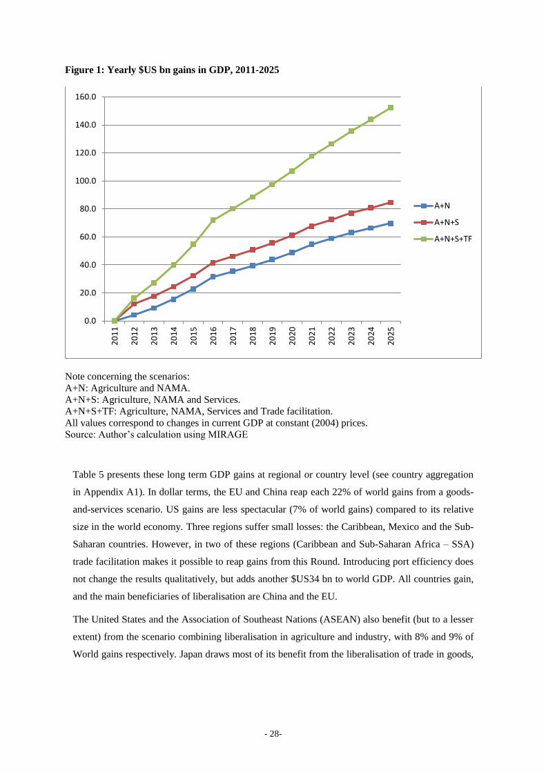
Figure 1: Yearly $US bn gains in GDP, 2011-2025

Note concerning the scenarios:

A+N: Agriculture and NAMA.

A+N+S: Agriculture, NAMA and Services.

A+N+S+TF: Agriculture, NAMA, Services and Trade facilitation.

All values correspond to changes in current GDP at constant (2004) prices.

Source: Author’s calculation using MIRAGE

Table 5 presents these long term GDP gains at regional or country level (see country aggregation

in Appendix A1). In dollar terms, the EU and China reap each 22% of world gains from a goods-

and-services scenario. US gains are less spectacular (7% of world gains) compared to its relative

size in the world economy. Three regions suffer small losses: the Caribbean, Mexico and the Sub-

Saharan countries. However, in two of these regions (Caribbean and Sub-Saharan Africa – SSA)

trade facilitation makes it possible to reap gains from this Round. Introducing port efficiency does

not change the results qualitatively, but adds another $US34 bn to world GDP. All countries gain,

and the main beneficiaries of liberalisation are China and the EU.

The United States and the Association of Southeast Nations (ASEAN) also benefit (but to a lesser

extent) from the scenario combining liberalisation in agriculture and industry, with 8% and 9% of

World gains respectively. Japan draws most of its benefit from the liberalisation of trade in goods,

0.0

20.0

40.0

60.0

80.0

100.0

120.0

140.0

160.0

20

11

20

12

20

13

20

14

20

15

20

16

20

17

20

18

20

19

20

20

20

21

20

22

20

23

20

24

20

25

A+N

A+N+S

A+N+S+TF

- 29-

reaping 15% of World gains in this scenario.14

The EU benefits most from liberalisation in services

(50% of world gains accrue to the EU27). SSA gains $US6.4bn of GDP from trade facilitation.

Table 5: Long run deviations from the baseline, GDP, $US mn

Goods + Services

+ Trade

Facilitation

Argentina 694 730 890

ASEAN 6,492 7,319 12,973

Australia& New Zealand 1,401 1,545 1,714

Brazil 366 456 2,044

Canada 859 1,197 1,302

Caribbean -718 -696 131

China 15,981 18,443 36,465

EFTA 7,289 7,669 7,669

European Union 11,847 18,571 30,731

India 3,821 4,328 6,932

Japan 10,194 10,703 13,772

Korea 635 887 4,512

Mexico -473 -353 -296

North Africa 1,062 1,150 1,279

Rest of Africa (except South

Africa) -549 -394 6,024

Rest of Mercosur 438 480 889

Rest of South America 977 1,057 2,533

Rest of South Asia 454 582 1412

Rest of World 1,001 1,809 7,390

Taiwan 2,498 2,622 4,524

USA 5,344 6,450 9,480

Note: Long run is 2025. Gains are in constant 2004 dollars, relative to 2025 economic values.

Source: Author’s calculation using MIRAGE

In addition to changes in the amounts of GDP, individual countries may be affected by terms of

trade changes and by efficiency gains or losses. This can be examined using the decomposition of

welfare changes in Table 6. Taiwan, Japan, the ASEAN and the North African countries benefit

from sizeable gains in allocative efficiency due to specialisation in activities in which they have

advantages. This contributes to the GDP gains observed earlier. However, for the North African

14

Detailed analysis reveals a very significant increase of Japanese car production as a result of Doha.

- 30-

countries these gains are reduced due to terms of trade losses, yielding an overall negative welfare

gain.15

Terms of trade are also adversely affected in Mexico and Canada, two countries that currently

generally benefit from the North-American Free Trade Agreement (NAFTA). However, only

Mexico experiences a welfare loss (-0.15% for Mexico, compared to 0.02% for Canada). Korea

experiences only a small improvement in welfare since most trade liberalisation applies in the

reference scenario which integrates the recent EU-Korea agreement.

Table 6: Decomposition of long run welfare gains (agric. + NAMA + services) (percentages)

Welfare

Allocation

efficiency

Capital

accumulation

Land

supply

Terms

of

trade Variety Other

Argentina 0.23 0.09 0.09 0.04 0.05 -0.03 -0.00

ASEAN 0.56 0.11 0.21 0.01 0.15 0.01 0.09

Australia& New Zealand 0.15 0.05 0.04 0.03 0.06 -0.02 -0.00

Brazil 0.03 0.07 0.01 0.02 0.02 -0.06 -0.04

Canada 0.02 0.06 -0.00 0.01 -0.03 -0.02 0.01

Caribbean -0.11 0.01 -0.02 0.01 0.04 -0.05 -0.11

China 0.19 0.04 0.10 0.00 0.06 0.01 -0.01

EFTA 0.84 0.66 0.09 -0.02 0.04 0.03 0.04

European Union 0.06 0.08 -0.00 -0.00 -0.06 0.00 0.05

India 0.15 0.06 0.04 0.00 0.01 0.01 0.02

Japan 0.32 0.09 0.03 -0.00 0.07 0.02 0.10

Korea 0.07 0.08 0.02 -0.00 -0.00 -0.07 0.04

Mexico -0.15 0.07 -0.03 0.01 -0.10 -0.03 -0.07

North Africa -0.13 0.19 -0.01 0.01 -0.18 -0.08 -0.07

Rest of Africa (except South Africa) -0.10 0.00 -0.02 0.00 -0.05 -0.02 -0.02

Rest of Mercosur 0.16 0.05 0.06 0.01 0.10 -0.00 -0.06

Rest of South America 0.21 0.02 0.08 0.04 0.07 -0.01 0.01

Rest of South Asia 0.14 0.02 0.05 0.01 0.06 0.01 -0.01

Rest of World -0.00 0.01 0.00 0.00 -0.03 0.00 0.00

Taiwan 0.44 0.24 0.10 0.00 0.01 0.03 0.07

USA 0.03 0.02 0.00 -0.01 -0.04 0.00 0.04

Source: Authors’ calculation using MIRAGE

The case of Sub-Saharan Africa is important for the Round and deserves additional comment. It

should be remembered that this region does not liberalise overall (or only to a very small extent),

due to the combined presence of LDCs, Paragraph 6 Annex b countries and other flexibilities

15

Due to the computation of GDP at constant prices, short-term GDP evolutions are not affected by terms of

trade. However, terms of trade affect a country’s capacity to invest, so they will translate into dynamic GDP

gains or losses in the long run.

- 31-

conceded to developing countries. In simple bilateral liberalisation schemes, it is usually assumed

that a country which opens less benefits from terms of trade gains, to the detriment of its partner.

In a multilateral framework however, things are not so simple. In particular, improved market

access is usually more limited for SSA countries, which already benefit from preferential schemes

in some important markets. The improved market access granted to SSA countries’ competitors

actually works to decrease some of the SSA countries’ export prices, leading to terms of trade

losses even in the absence of liberalisation. This could result in reduced domestic production in

several industries, increased average costs and less variety for local and foreign consumers.

However, the introduction of trade facilitation yields very large welfare gains for the SSA region

(up to 0.5% of GDP). Nevertheless, these results are very conservative compared to Minor and

Tsigas’s (2008) estimates, which show GDP gains of 1.1% to 4.2%.

While a reduction in tariff barriers generally deteriorates terms of trade for the opening economy,

the converse is true when a country facilitates imports. Trade facilitation data and our scenario

assumption suggest that a trade facilitation programme in the SSA countries would mostly reduce

the time to import goods, making imported goods cheaper for importers compared to exported

goods. Hence, terms of trade gains improve (+0.1%) if trade facilitation is added, as shown in

Table 7. In the absence of trade facilitation, terms of trade are deteriorating for this region. Also,

capital accumulation is encouraged and contributes to half of the recorded welfare gains for SSA.

The inclusion of port efficiency in our scenario adds to the expected outcomes. The results (not

reported here) show that welfare would increase by more than 0.8% in SSA, driven mainly by

allocation efficiency and capital accumulation gains.

- 32-

Table 7: Decomposition of long run welfare gains (agric. + NAMA + services + TF), percentages

Of which:

Welfare Allocation

efficiency

Capital

accumulation

Land

supply

ToT Variety Trade-cost

(exporter)

Argentina 0.24 0.08 0.09 0.04 0.03 -0.03 0.04

ASEAN 0.84 0.13 0.31 0.01 0.13 0.03 0.15

Austr. New Z 0.13 0.05 0.04 0.03 0.03 -0.03 0.01

Brazil 0.10 0.08 0.04 0.03 -0.01 -0.06 0.05

Caribbean 0.04 0.02 0.01 0.01 0.05 -0.04 0.04

China 0.40 0.05 0.20 0.00 0.14 0.04 0.03

EFTA 0.78 0.66 0.08 -0.02 -0.00 0.03 0.03

EU 0.12 0.08 0.01 -0.00 -0.07 0.00 0.05

India 0.24 0.07 0.06 0.00 0.02 0.01 0.03

Japan 0.35 0.10 0.04 -0.00 0.05 0.02 0.05

Korea 0.27 0.10 0.06 -0.00 -0.12 -0.05 0.17

Mexico -0.16 0.07 -0.03 0.02 -0.11 -0.03 0.01

North Africa -0.17 0.20 -0.01 0.01 -0.21 -0.08 0.02

Canada -0.00 0.06 -0.01 0.01 -0.06 -0.02 0.02

Rest of Africa 0.45 0.07 0.22 0.01 0.07 0.03 0.04

R.o Mercosur 0.22 0.06 0.08 0.01 0.11 -0.00 0.05

R. o South Am. 0.41 0.03 0.15 0.05 0.07 -0.00 0.09

R. o South Asia 0.28 0.03 0.09 0.01 0.08 0.01 0.05

R. o World 0.05 0.03 0.03 0.00 -0.05 0.00 0.04

Taiwan 0.64 0.26 0.13 0.00 -0.14 0.07 0.23

USA 0.05 0.02 0.00 -0.01 -0.03 0.01 0.01

Source: Authors’ calculation using MIRAGE

- 33-

7. Sectoral impact of the central scenario

We should also discuss some sectoral and regional results of a central scenario combining

liberalisation in agriculture and services as defined above, with the NAMA and trade facilitation.

Table 8 shows changes in the value of exports for the different regions in the three broad sectors of

interest: agriculture, industry and services.

In agriculture, the two main beneficiaries of the DDA in terms of exports are the EU (+$US9.8 bn)

and Australia and New Zealand (+$US8.3bn). Brazil also gains in agriculture in this Round (+$US

6.7 bn). The strong specialisation of Australia, New-Zealand, Brazil and to some extent Canada in

agriculture, implies that the bulk of their export gains are concentrated in this sector. The second

largest gains in industrial exports are in the EU (+$US 53 bn or 18% the increase in world exports

in this sector), followed by Japan (+$US 40 bn) and the US (+$US 38bn). The largest gainer in

industry will be China (+67.8 bn), but the EU will export an additional $US 15.4 bn of services,

representing more than half of the increase in world trade in services, a sector where Chinese

exports will stagnate. Other regions with major increases in exports of industrial products are

Japan (+$US 40.1 bn), the USA (+$US 38.1 bn) and other Asian countries (ASEAN, Korea and

Taiwan together represent a larger gain than the EU). In services, the US is the only other country

to achieve sizeable gains (+$US 8.4 bn).

Table 9 shows the combined impacts of changes in exports, imports and demand, for every broad

sector. Changes in production are deduced from these three components. Internal demand is less

sensitive than trade to price changes, and generally represents a large proportion of total demand.

Consequently, changes in production are cushioned compared to trade variations. It is interesting

that not both production and content in terms of intermediate inputs adjust. Accordingly, we need

to consider changes in value added by sector.

- 34-

Table 8: Long run change in the value of exports (Goods + Services + TF), $US bn

Agriculture Industry Services

Argentina 1.65 -0.16 0.08

ASEAN 3.48 25.95 -3.48

Australia& New Zealand 8.35 1.28 0.29

Brazil 6.70 1.13 0.13

Canada 4.27 -2.47 1.50

Caribbean 0.76 0.79 -0.06

China 1.68 67.78 -0.70

EFTA 0.58 3.75 1.86

European Union 9.78 52.98 15.41

India 0.53 8.65 0.12

Japan 0.63 40.13 -3.30

Korea 0.29 20.86 -0.31

Mexico 0.69 2.19 0.51

North Africa 1.42 4.57 2.34

Rest of Africa (except South Africa) 0.75 5.72 0.77

Rest of Mercosur 0.34 1.40 0.13

Rest of South America 2.28 0.80 -0.06

Rest of South Asia 0.31 1.80 -0.15

Rest of World 1.47 5.19 4.17

Taiwan 0.14 10.50 -0.35

USA -2.38 38.06 8.35

World 43.70 290.91 27.24

Source: Authors’ calculation using MIRAGE

Note: Long run is 2025. Gains are in constant (2004) dollars, relative to 2025 economic values.

- 35-

Table 9: Long run percentage changes in value added by broad sector (Goods + Services + TF)

Agriculture Industry Services

Argentina 3.43 -0.80 0.31

ASEAN 1.04 1.08 0.66

Australia & New Zealand 6.93 -0.92 0.24

Brazil 4.24 -1.04 0.17

Canada 3.29 -0.25 0.17

Caribbean 1.60 -0.24 0.02

China 0.49 0.32 0.56

EFTA -18.68 1.11 0.96

European Union -0.70 0.27 0.33

India 0.35 0.19 0.37

Japan -3.79 1.10 0.32

Korea 0.03 1.16 0.56

Mexico 1.18 -0.20 -0.03

North Africa 1.61 0.42 0.39

Rest of Africa (except South

Africa) 0.80 -0.27 0.69

Rest of Mercosur 0.99 0.32 0.08

Rest of South America 2.58 -0.44 0.35

Rest of South Asia 0.52 0.25 0.18

Rest of World 0.38 -0.05 0.26

Taiwan 1.25 0.98 0.93

USA -0.26 0.27 0.13

Source: Author’s calculation using MIRAGE

In terms of overall agricultural value added, Australia and New Zealand benefit the most from

increased exports because they are more open to international trade (+6.9%). Argentina, Canada

and Brazil (3.3% and 4.2% increases) are ranked next. EU value added reduces by -0.7%. Japan

experiences a significant decrease in agricultural value added of -3.8%. Due to their very strong

initial protection, the EFTA countries face the strongest reduction for agriculture value added (-

18.7%) and reorient their resources toward the other sectors. China and India are hardly affected.

In aggregate industry, all variations of regional level value added are in the range +/-1%, the main

winners being ASEAN, Japan and Korea. Australia, New-Zealand and Brazil show value added

losses in this sector, compensating for their gains in agriculture. Canada, the Caribbean countries

and Mexico are also negatively affected by losing their initially favourable access to the US

market for industrial goods. Asia is the largest gainer from these changes. The US and European

industries show a +0.3% increase in value added thanks to the further openness of foreign markets

(as big as that for China).

Value added in services is less affected, with variations of less than 1% (in absolute terms) as a

result of the Round’s limited ambitions for services.

- 36-

The results by broad sector are detailed in Appendix 3, for each region and each sector. In terms of

agriculture value added, the largest negative shocks are in the EFTA countries (meat: -43.0%;

sugar -26.4%; fibres and crops -21%; vegetable and fruits -22.0%; cereals -19.5%). Some of this

effect is compensated for by an increase in oil and fats value added (+14.1%). These results are a

direct result of the initial level of protection for agriculture in this region. In countries benefiting

from a comparative advantage in agriculture, increases in value added are large: Australia and

New-Zealand show an increase in value added in every sector of agriculture. It is below 3% for

vegetable and fruits, oils and fats, and sugar, but between 5% and 6% for fibres, cereals and meat,

and +24.1% for dairy products. North Africa benefits from improved market access for oil and fats

(+22.4%). Brazil’s and Argentina’s trade barriers for meat and Brazil’s trade barriers for fibre, are

reduced resulting in a visible increase in value added for these sectors (meat: +7.9% in Brazil and

+7.0% in Argentina; fibres: +7.0% and + 2.8% respectively).With some exceptions the figures are

not so large, especially if we keep in mind that these are deviations from the baseline and that

agricultural production should increase at the horizon on the baseline for food and agro-industry

purposes. Changes in EU value added in different agricultural sectors are smaller, with the

exception of sugar (-12.9%). For vegetable and fruits, fibres and crops, cereals, dairy, and even

meat, changes are below 2% for the EU, but oils and fats show a drop of -4.2% over the long run.

When considering these figures, it should be noted that we are measuring deviations from a

baseline that comprises increased demand for agricultural products at the European and world

levels, as a result of economic growth.

The effects of industry value added changes are seen mainly in labour intensive activities in North

America, Australia and New Zealand, Canada and Mexico. In textile and clothing, value added

reduces by -21.5% in Australia and New Zealand, -17.2% in Canada, -11.4% in the USA, and -

8.8% in Mexico. The largest shifts in value added at the world level are in the industrial sector.

Countries specialising in this sector are the Caribbean (+7.8%, to serve the NAFTA countries) and

Asia (Taiwan +32.1%, Korea +11.1%, ASEAN +7.3%, China +5.6%).

The next most affected sector is automobiles, to the benefit of Japan, which is specialised in this

sector (+12.2%). India is ranked next, with a 1.3% increase in value added in this sector. Australia

and New Zealand lose value added in automobiles (-10.4%), the reverse of the large gains in the

agricultural sector. Assembly lines in North Africa, Canada, Brazil and Argentina shrink

moderately (between -3% and -4%). The impact on the European car industry is limited (-2.1%)

compared to the recent shocks experienced in this sector. Other changes are below two digit

figures in every pair region-sector, pointing to a limited impact of the Round on industrial value

added when imports and exports are considered jointly for every region, making the Round easier

to conclude on political grounds. In services, the changes are virtually not visible provided that

liberalisation is limited.

- 37-

8. Central scenario: Detailed impacts on factor incomes

The changes in specialisation and related changes in value added induce displacement of workers

across sectors, and a progressive reorientation of the capital stock towards the most competitive

activities. Since not all activities displace or attract skilled and unskilled workers in equal

proportions, there will be excess demand (or supply) in a given type of labour which will translate

into an increase (decrease) in related wages. This mechanism is based on the assumption of a

flexible labour market and no unemployment. Note that substitutions will occur not only between

skills, but also between factors (e.g. capital substituted by labour). These substitutions cushion the

changes in factor returns, with factors in less demand becoming relatively cheaper and more

intensively used.

Against this theoretical setting, we can examine the extent of factor displacement in the long run,

after adjustments. Table 10 shows the displacement of workers (unskilled and skilled) across broad

activities. With the exception of agriculture in the EFTA countries, displacements are limited and

work force percentages remain under two digits. Within the EU, displacements are a maximum of

1% in each broad sector and for each category of workers. These figures reflect regional

specialisation advantages: in Argentina, Australia and New Zealand, Canada, the Caribbean,

Mexico and Africa employment of both skilled and unskilled workers increases in agriculture, but

decreases in industry. The pattern is reversed for China, Japan and Korea. With the exception of

the EFTA, the trend is towards lower displacement in agricultural employment than the changes

driven by demographic changes and the progressive shift towards service economies. However,

displacement will be more pronounced in certain activities in a given sector, for example the case

of sugar in the EU (see Table 11).

- 38-

Table 10: Long run percentage changes in employment by sector (central scenario)

Agriculture Industry Services

Skilled Unskilled Skilled Unskilled Skilled Unskilled

Argentina 2.49 2.79 -1.61 -1.85 0.10 -0.09

ASEAN 0.55 -0.11 0.76 0.83 -0.23 -0.50

Australia & New Zealand 6.37 6.35 -2.45 -3.05 0.06 -0.19

Brazil 3.12 3.66 -1.29 -1.37 0.03 -0.02

Canada 2.48 3.11 -0.51 -0.91 0.02 0.02

Caribbean 0.61 1.02 -0.10 -0.09 -0.01 -0.21

China -0.06 -0.15 0.28 0.13 -0.08 -0.05

EFTA -17.68 -20.70 0.87 1.18 0.07 0.29

European Union -0.88 -1.01 0.02 -0.07 0.02 0.13

India 0.11 -0.01 0.00 -0.11 -0.01 0.04

Japan -3.29 -4.05 0.94 0.74 -0.15 -0.02

Korea -0.47 -0.36 0.23 0.33 -0.05 -0.09

Mexico 0.25 0.82 -0.22 -0.56 0.02 -0.13

North Africa 0.98 1.39 -2.09 -2.31 0.16 0.22

Rest of Africa (excl. S. Africa) 0.03 0.17 -0.68 -0.82 0.05 0.08

Rest of Mercosur 0.70 0.87 -0.81 -0.87 0.11 0.18

Rest of South America 1.22 1.85 -1.17 -1.47 0.04 -0.11

Rest of South Asia 0.39 0.11 0.46 0.39 -0.03 -0.09

Rest of World 0.02 0.15 -0.29 -0.35 0.02 0.06

Taiwan -0.55 0.07 -0.13 0.24 0.05 -0.15

USA -0.17 -0.60 0.28 -0.11 -0.04 0.04

Source: Authors’ calculation using MIRAGE

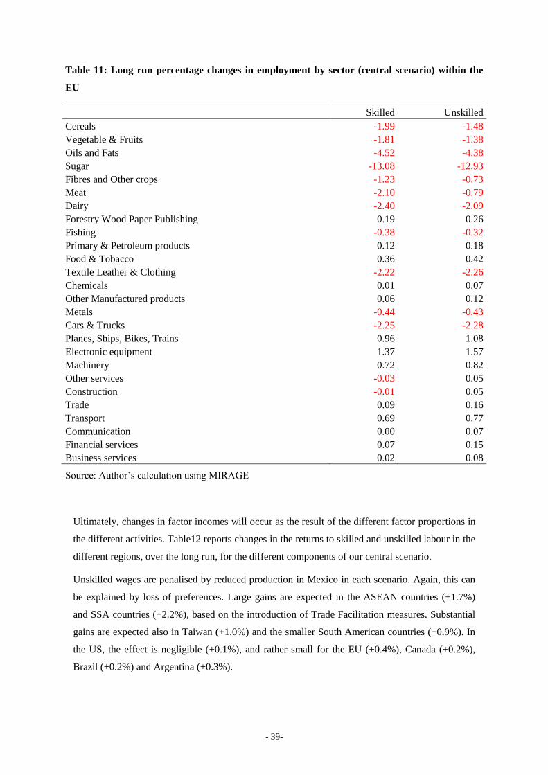
- 39-

Table 11: Long run percentage changes in employment by sector (central scenario) within the

EU

Skilled Unskilled

Cereals -1.99 -1.48

Vegetable & Fruits -1.81 -1.38

Oils and Fats -4.52 -4.38

Sugar -13.08 -12.93

Fibres and Other crops -1.23 -0.73

Meat -2.10 -0.79

Dairy -2.40 -2.09

Forestry Wood Paper Publishing 0.19 0.26

Fishing -0.38 -0.32

Primary & Petroleum products 0.12 0.18

Food & Tobacco 0.36 0.42

Textile Leather & Clothing -2.22 -2.26

Chemicals 0.01 0.07

Other Manufactured products 0.06 0.12

Metals -0.44 -0.43

Cars & Trucks -2.25 -2.28

Planes, Ships, Bikes, Trains 0.96 1.08

Electronic equipment 1.37 1.57

Machinery 0.72 0.82

Other services -0.03 0.05

Construction -0.01 0.05

Trade 0.09 0.16

Transport 0.69 0.77

Communication 0.00 0.07

Financial services 0.07 0.15

Business services 0.02 0.08

Source: Author’s calculation using MIRAGE

Ultimately, changes in factor incomes will occur as the result of the different factor proportions in

the different activities. Table12 reports changes in the returns to skilled and unskilled labour in the

different regions, over the long run, for the different components of our central scenario.

Unskilled wages are penalised by reduced production in Mexico in each scenario. Again, this can

be explained by loss of preferences. Large gains are expected in the ASEAN countries (+1.7%)

and SSA countries (+2.2%), based on the introduction of Trade Facilitation measures. Substantial

gains are expected also in Taiwan (+1.0%) and the smaller South American countries (+0.9%). In

the US, the effect is negligible (+0.1%), and rather small for the EU (+0.4%), Canada (+0.2%),

Brazil (+0.2%) and Argentina (+0.3%).

- 40-

The wages for skilled workers increase almost everywhere (with the exception of Brazil where

they are stable) when the effects of liberalisation in agriculture, industry, services and trade

facilitation are combined. The gains small in Korea 0.6%, in the US, Australia and New-Zealand

0.2% and in the EU 0.4%. Trade facilitation benefits the SSA and ASEAN countries the most,

with gains of 2.3% and 1.3% respectively.

In countries specialised in agriculture, such as Australia, New Zealand and Canada, and also in

South America, the returns to land increase by at least 2% in the long run (up to 3% in Brazil and

3.6% in Canada). This contrasts with the decrease in the returns to land for the US, EU and Japan

(-7% on average), and the huge 39% decrease for EFTA. Real returns to land in Asia and India are

barely affected in any of the scenarios: changes never exceed 1% in absolute terms. Changes in the

returns to capital are limited throughout these regions, and never reach 1%.

- 41-

Table 12: Long run percentage changes in real wages

Skilled

Unskilled

Goods

+

Services

+ Trade

Facilitation Goods

+

Services

+ Trade

Facilitation

Argentina 0.17 0.19 0.17 0.30 0.32 0.29

ASEAN 0.56 0.64 1.33 0.87 0.91 1.20

Australia &

New Zealand 0.09 0.11 0.19 0.37 0.40 0.46

Brazil -0.11 -0.11 0.02 0.01 0.02 0.13

Canada 0.01 0.04 0.13 0.03 0.05 0.14

Caribbean -0.18 -0.17 0.09 0.11 0.11 0.25

China 0.40 0.43 0.87 0.44 0.46 0.71

EFTA 1.30 1.37 1.42 0.68 0.74 0.78

European Union 0.13 0.18 0.38 0.06 0.10 0.22

India 0.24 0.26 0.30 0.23 0.25 0.24

Japan 0.57 0.59 0.68 0.35 0.36 0.43

Korea 0.27 0.32 0.59 0.39 0.42 0.59

Mexico -0.24 -0.24 -0.23 -0.09 -0.07 -0.07

North Africa -0.11 -0.10 0.63 -0.14 -0.13 0.62

Rest of Africa

(except South

Africa)

-0.18 -0.16 2.28 0.01 0.01 1.85

Rest of Mercosur 0.02 0.05 0.10 -0.08 -0.06 -0.05

Rest of South Am. 0.13 0.15 0.43 0.26 0.29 0.48

Rest of South Asia 0.09 0.13 0.32 0.12 0.16 0.29

Rest of World -0.01 -0.00 1.20 -0.01 -0.01 1.19

Taiwan 0.64 0.64 0.95 0.68 0.68 0.91

USA 0.11 0.12 0.20 0.01 0.03 0.08

Note concerning the scenarios:

A+N: Agriculture and NAMA.

A+N+S: Agriculture, NAMA and Services.

A+N+S+TF: Agriculture, NAMA, Services and Trade facilitation

Source: Authors’ calculation using MIRAGE

- 42-

9. Impact of sectoral initiatives

In three broad sectors (chemicals, machinery, electronics) several WTO members are keen to open

global markets further (excluding LDCs) through sectoral initiatives. There is also a separate

initiative for environmental goods. In our analysis, we make the assumption that these initiatives

will be endorsed by all developed countries (including Korea) and also (we assume optimistically)

a number of developing countries, such as Argentina, Brazil, Chile, Colombia, Peru, Paraguay,

Uruguay, Mexico, China, India, Indonesia, Malaysia, Philippines, Taiwan and Thailand.16

For chemicals, the more ambitious proposal is to reach the level of protection defined in the 1995

plurilateral CTHA; for machinery and electronics, the ambition is for zero bound tariffs. Tariff

reductions are not welcomed, therefore, by the emerging countries, and a second proposal has been

advanced by the EU, which allows developing countries more room for manoeuvre. The following

is based on this second approach since the first proposal stands little chance of endorsement by all

WTO members. Not all duties on corresponding products are set to zero after the five years

implementation period because developing countries are allowed to keep in place some protection.

For chemicals, developed countries’ tariffs are reduced to zero in five years; for developing

countries there is a 10 year implementation period. Development countries also can leave 4% of

their tariffs bound at 4% (within a trade volume limit of 4%). A further 5% of tariffs can be

reduced to zero over 15 years.

For electronic products, developed countries’ tariffs are brought to zero in three years.

Developing countries are granted a five year implementation period and they can leave 5% of their

tariffs bound at 5%, provided these lines do not exceed 5% of the total value of the member's

imports of covered products.

Last, for machinery, developed countries’ tariffs are brought to zero in four years. Developing

countries have seven years to implement the tariff cut and can leave 4% of their tariff lines at 5%,

provided they do not exceed 5% of the total value of the member's machinery imports.

The sectoral initiative on environmental goods refers to the official list of environmental products

used in WTO negotiations. Here, tariffs on these products are set at zero. In a less strict version of

the environmental simulation, removal of the tariffs on products identified as environmental is

replaced by application of a more demanding Swiss formula than for other NAMA tariff lines.

In our exercise, countries apply the sectoral initiative first, and choose their sensitive products

afterwards. Goods included in these sectoral initiatives cannot be considered sensitive by

developing countries. Thus, sensitive products must be chosen in a second step, possibly in less

protected sectors, which adds to the initial effects of the initiatives.

16

Recall that in the WTO arena, Korea is considered a developed country for industrial goods, but not for

agricultural goods.

- 43-

Table 13, column (1) presents the long run changes in world trade of agricultural and industrial

goods and services compared to the baseline, associated with the three pillars of the negotiation in

agriculture and the NAMA. The $US2.6bn increase in trade in services is a pure general

equilibrium effect.

Table 13: Long run changes in trade volumes ($US bn)

(1) (2) (3) (4) (5) (6) (7)

Agric+NAMA Services

Trade

facilitation

Port

efficiency

Mach-

Chem-

Electn.

Envt.

zero

Swiss

4-10/11

on envt

Agriculture 32.28 32.51 36.70 38.83 37.83 36.86 36.75

Industry 194.94 195.95 285.41 330.30 430.96 308.96 290.90

Services 2.61 35.23 36.42 37.28 36.41 36.27 36.38

Note: (1) agriculture + NAMA; (2) agriculture + NAMA + services; (3) agriculture + NAMA +

services + trade facilitation; (4) agriculture + NAMA + services + trade facilitation + port efficiency;

(5) agriculture + NAMA + services + trade facilitation + sectorals except environmental goods; (6)

agriculture + NAMA + services + trade facilitation + zero tariffs initiative on environmental goods; (7)

agriculture + NAMA + services + trade facilitation + more demanding Swiss formula on

environmental goods.

Source: Authors’ calculation using MIRAGE

Table 13, column (2) includes limited liberalisation in services. Again, we observe small general

equilibrium effects on trade in goods. Column 3 shows the central scenario. The impact of trade

facilitation is shared among agricultural and industrial goods, and general equilibrium effects on

trade in services are visible again. Columns 4, 5, 6 and 7 must be compared to Column (3).

Column (4) reports the results for port efficiency; Column (5) shows the $US145.6 bn increase in

trade in industrial goods when the first sectoral initiative (chemicals, machinery, electronics) is

added. The general equilibrium effects on agriculture are still visible, though limited, and there is

no effect on trade in services. In Column 6, the first version of the sectoral initiative on

environmental goods is added to the central scenario. Its impact on trade is negligible overall

($US23.6 bn or an additional 8%), compared to the central scenario. Gains are in line with the

limited product coverage of this proposal (168 HS6 lines compared with machinery 430,

electronics 440 and chemicals 910 lines). Column (7) relies on a softer version of the

environmental simulation in which the removal of tariffs on products identified as environmental

is replaced by the application of a more demanding Swiss formula than for the rest of the NAMA.

- 44-

This approach makes only very small differences overall. This outcome is the result of limited

coverage of the list of affected products.

Table 14 examines how the results in Columns 5, 6 and 7 translate into changes in GDP for the

regions. First we consider the effects of the sectoral initiative on chemicals, machinery and

electronics. The overall additional GDP gain is $US17bn in this scenario ($US169 bn compared to

$US152bn for the central scenario). In terms of GDP, the additional effects of the sectoral scenario

are concentrated in a limited number of winners in Asia (Taiwan, ASEAN, Korea, China and to a

lesser extent Japan) plus Mexico (taking advantage of the further opening of markets in the

region), and China and Taiwan.

The environmental goods initiative adds less than $US2bn to world GDP in the long run when a

zero tariff initiative is adopted.

Lastly, replacing this zero initiative with an ambitious Swiss formula has no visible impact on

GDP, due to the quasi-absence of an impact on trade.

- 45-

Table 14: Long run changes in GDP ($US mn)

(1) (2) (3) (4) (5) (6) (7)

Agric+NAMA Services

Trade

facilitation

Port

efficiency

Mach

Chem

Electr

Envt

zero

Envt

Swiss

4-10/11

Argentina 694 730 890 952 893 890 893

ASEAN 6,492 7,319 12,973 16,840 15,534 15,727 15,595

Australia

& New

Zealand 1,401 1,545 1,714 1,979 1,830 1,868 1,843

Brazil 366 456 2,044 2,296 1,960 1,958 1,963

Canada 859 1,197 1,302 1,320 1,266 1,267 1,268

Caribbean -718 -696 131 234 260 266 263

China 15,981 18,443 36,465 39,815 42,309 42,738 42,407

EFTA 7,289 7,669 7,669 7,688 7,819 7,820 7,819

EU 11,847 18,571 30,731 34,931 33,789 33,976 33,824

India 3,821 4,328 6,932 8,525 4,481 4,612 4,521

Japan 10,194 10,703 13,772 14,869 15,472 15,684 15,519

Korea 635 887 4,512 5,125 5,424 5,408 5,422

Mexico -473 -353 -296 -416 1,681 1,639 1,682

North

Africa 1,062 1,150 1,279 1,158 1,116 1,259 1,166

Rest of

Africa -549 -394 6,024 10,866 6,057 6,043 6,056

Rest of

Mercosur 438 480 889 2,837 923 934 926

Rest of

South

America 977 1,057 2,533 4,769 2,850 2,930 2,866

Rest of

South

Asia 454 582 1,412 2,026 1,329 1,373 1,351

Rest of

World 1,001 1,809 7,390 15,236 7,272 7,434 7,284

Taiwan 2,498 2,622 4,524 4,754 5,920 6,037 5,947

USA 5,344 6,450 9,480 11,054 11,012 11,106 11,031

World 69,615 84,552 152,370 186,857 169,198 170,970 169,648

Source: Authors’ calculation using MIRAGE

- 46-

10. Our results compared with those in the related literature

We compare our results with the results from studies that rely on similar methodologies: a paper by

Francois et al. (2005) and three by Bouët and Laborde (2009-a, 2009b, 2010). Table 15 compares

these studies which rely on CGE models. Interested readers can find additional references in

Piermartini and Teh (2005) for CGE studies on the DDA from 2003 to 2005.We present the basic

features of the models and the simulation results for world GDP and world exports from the selected

studies.

Results differ because of different modelling assumptions (static versus dynamic version through

capital accumulation). The base years differ and different scenarios are simulated. A convenient

feature of these studies, however, is that they all rely on the GTAP database (version 6 or 7) and thus

correctly benchmark our results (although we use a more recent version of this dataset). Direct

comparison of results would be misleading, but we can check whether results converge.

Francois et al. proposed various versions of their model. Here, we refer to Francois et al. (2005). It

models two scenarios: a 50% linear reduction in all the measures and a 1.5% reduction in trade costs

in anticipation of future work on trade facilitation, and an OECD-based Trade Round where cuts apply

only to OECD countries. They obtain a 5% to 11% increase in world trade and a 0.3% to 0.5%

increase in world GDP.

Bouët and Laborde (2009) find that following the conclusion of the Doha Round in July 2008, world

exports will grow by 1.46% in 2025 or $US336 bn compared to the situation without agreement.

World GDP will grow by 0.09%, adding $US59 bn from 2025 onwards. Their simulation does not

include services or trade facilitation, and among the scenarios we simulated the one that is closest to

this gives an increase of 1.25% in world exports, and an increase of 0.09% in world GDP. Although

our model assumptions are different (e.g. market structure), our results are not very different from

theirs. Their study is original in the sense that they measure what would be the consequence of a Doha

Round failure. To them, failure of the Round would materialise in a worldwide increase in tariffs (up

to the tariff bound, for instance). Results show that, were that the case, trade would be reduced by

-10%, and welfare would be down by -0.51%.

Bouët and Laborde (2009b) estimate possible outcomes of the Doha Round in the context of failure in

the Cancun discussions. They use a static version of the MIRAGE model and simulate 143 different

trade shocks, which fall into five categories: import duty cuts, degree of harmonisation adopted in the

tariff-reduction formula, provision of Special and Differential Treatment (SDT), global versus sectoral

negotiation, and export subsidies. The scenario that maximises world output includes liberalisation in

services, an ambitious Swiss formula without SDT, and a 75% reduction in export subsidies. In this

scenario, world output grows by 0.41%, equivalent to a gain of $US127 bn. One of the main

conclusions of their study is that agriculture is a key element of negotiations: it increases expected

- 47-

gains for small countries. However, Bouët and Laborde stress that some countries might lose from

international trade, due preference erosion and an increase in world agriculture prices. This last

emerges from our simulation results.

Bouët and Laborde (2010) examine five scenarios, namely the 2003 proposals from WTO chairs, the

October 2005 G-20 proposal, the EU's contribution in October 2005, the US 2005 proposal and the

December 2008 modalities. They show that the December 2008 package would reduce average tariffs

by 25%, a reduction very close to that implied by the 2003 Harbinson and Girard proposals. This

should be compared with the 73% reduction in world agricultural protection by the very ambitious

2005 US proposal. The 2005 G-20 and EU proposals, then, are intermediate proposals. Different

scenarios imply losses for developing countries, reflecting eroding preferences and rising terms of

trade for imported commodities, including food products. However, on the whole, world exports

should increase in the range 2% to 3.7% and world GDP 0.0% to 0.24%.

- 48-

Table 15: Selected CGE assessments of the DDA

- 49-

11. Conclusion

The exercise in this report is based on an updated version of the negotiated DDA draft modalities.

It proposes a representation of the impact of liberalised market access and reduction in farm

support, taking account of the various formulas, exceptions and flexibilities. In the absence of

more detailed information on the possible outcome of negotiations on these issues, we add a

reduction in trade barriers in services. Trade facilitation, port efficiency, sectoral initiatives and

sectoral initiatives in NAMA are considered. These shocks to the world economy are introduced in

MIRAGE, a dynamic CGE model, and we compare the trajectory of the world economy to 2025,

to a dynamic baseline in the absence of final agreement in the Round. We provide results for 21

regions and 26 sectors of the world economy.

Given the political economy of the negotiations, various exceptions and flexibilities limit the

impact of the Swiss formula on manufacturing, and of the tiered formula on agriculture. Also,

several countries are exempt from liberalisation. However, the final mix of rules and exemptions

submitted by the chair persons would lead to a non-negligible impact on the world economy and

also to a positive outcome in terms of GDP for all regions, if not a systematic welfare gain.17

Our

simulations point to a $US70 bn world GDP gain if agriculture and industry were to be liberalised.

Moderate liberalisation in services would add another $US15 bn to world GDP over the long run.

These gains would be added to world GDP every year over the long run compared to the situation

without agreement. In addition, trade facilitation would result in some $US67 bn gains each year

to world GDP over the long term, and port efficiency would add a further $US35 bn. However, we

modelled gains, not the costs of the facilitation programme: its success will be conditional on the

finalisation of a costly Aid for Trade package. Sectoral initiatives do not add much to world gains.

There are three caveats to this. Firstly, the final outcome of the negotiation may include additional

items not modelled here. This is the case for modes 3 and 4 of the General Agreement on Trade in

Services (GATS), an increase in business security and transparency due to additional commitments

and lower bindings, an improvement in the rules managing world trade. Secondly, the cost of not

signing a final agreement is not just reversal of the gains computed here; an agreement around

current proposals would significantly lower bound tariffs and would extend the consolidation

coverage (Bouët and Laborde, 2008). Also, a move towards regionalism and bilateralism would be

unavoidable in the case of failure of the Round, with associated trade diversion effects. Thirdly,

the credibility of the regulatory architecture developed under the umbrella of the WTO would be

put at risk were negotiations to fail.

17

Mexico gains in terms of GDP when sectoral initiatives are considered. Other regions systematically gain

when trade facilitation is included.

- 50-

1. References

Anderson, J. E. (1979), A Theoretical Foundation for the Gravity Equation, American Economic

Review, 69: 106-116.

Asia Pacific Economic Co-operation (APEC) (1999), Assessing APEC Trade Liberalization and

Facilitation: 1999 Update, Economic Committee, September 1999. Singapore.

Asia Pacific Foundation of Canada (1999), Survey on Customs, Standards and Business Mobility

in the APEC Region. APF Canada: Vancouver.

Baier S. L., Bergstrand, J.H. (2001), The Growth of World Trade: Tariffs, Transport Costs, and

Income Similarity, Journal of International Economics, 53(1): 1-27.

Bergstrand J.H. (1990), The Heckscher-Ohlin-Samuelson Model, the Linder Hypothesis and the

Determinants of Bilateral Intra-industry Trade, Economic Journal, 100(403): 1216-29.

Bergstrand J.H.. (1989), The Generalized Gravity Equation, Monopolistic Competition, and the

Factor-Proportions Theory in International Trade, The Review of Economics and Statistics,

71(1):143-53.

Bouët A., Decreux Y., Fontagné L., Jean S. Laborde D. (2008), Assessing Applied Protection

Across the World, Review of International Economics, 16(5): 850-863.

Bouët A., Laborde, D. (2009-a), The Potential cost of a failed DOHA round, IFPRI discussion

paper, 886.

Bouët A., Laborde D. (2009-b), Why is the Doha Development Agenda Failing? And What Can be

Done? IFPRI Discussion Paper, 877.

Bouët A., Laborde D. (2010), Eight Years of Doha Trade Talks, IFPRI Disscussion Paper, 997.

Decreux Y., Ramos M.P. (2007), How does Tariff-rate quota modelling affect CGE results? An

application for MIRAGE, TradeAg Working Paper 2007-16.? Not in text

Dennis A. (2006), The Impact of Regional Trade Agreements and Trade Facilitation in the Middle

East North Africa Region, World Bank Policy Research Working Paper 3837.

Djankov S. Freund C., Pham, C.S. (2006), “Trading on Time,” World Bank, January.

Dutt P., Traca D., (2007), Corruption and Bilateral Trade Flows: Extortion or Evasion? Working

Paper, INSEAD.

Duval Y. (2006), Cost and Benefits of Implementing Trade Facilitation Measures under

Negotiations at the WTO: an Exploratory Survey, Working Papers 306, Asia-Pacific Research and

Training Network on Trade.

- 51-

Fontagné L, Fouré J., Ramos M.P. (2011), A new baseline for MIRAGE, Working Paper , CEPII,

Paris forthcoming.? Not in text

Fontagné L., Guillin A., Mitaritonna, C. (2011), Estimations of Tariff Equivalents for the Services

Sectors, CEPII Working Paper, forthcoming.

Fouré J., Bénassy-Quéré A., Fontagné, L. (2010), The World Economy in 2050: a Tentative

Picture, Working Papers 2010-27, CEPII, Paris.

Fox A., Francois J., Londono-Kent, P. (2003), Measuring Border Crossing Costs and their Impact

on Trade Flows: The United States-Mexican Trucking Case. Document presented at the sixth

conference on Global Economic Analysis. Den Haag.

Francois J., van Meil H., van Tongeren F.(2003), Economic Benefits of the Doha Round for the

Netherlands. Project Report.Den Haag: Agricultural Economics Research Institute.

Francois J., van Meil H., van Tongeren F.(2005), Trade liberalization in the Doha Development

Round, Economic Policy.

Freund C., Weinhold D. (2000), On the Effect of the Internet on International Trade, International

Finance Discussion Papers, No. 693, Board of Governors of the Federal Reserve System.

Gouel C., Guillin A., Ramos M.P. (2008), The Effects of Agricultural Policies on Developing

Countries at a Detail Level, TradeAg Working Paper 2008.? Not in text

Hertel T., Walmsley T., Itakura K. (2001), Dynamic Effect of the "New Age" Free Trade

Agreement between Japan and Singapore. Journal of Economic Integration 16, (4): 446- 84.

Hoekman B., Konan D. (1999), Deep Integration, Nondiscrimination, and Euro-Mediterranean

Free Trade. World Bank Policy Research Working Paper no. 2130. Washington: World Bank.

Hummels D. (2001), Time as a Trade Barrier, Mimeo, Department of Economics, Indiana: Purdue

University.

Jean S., Laborde D., Martin W. (2008), Choosing Sentitive Agricultural Products in trade

Negotiations , CEPII working paper, 2088-18.

Kee H.L., Nicita A., Olarreaga M. (2008), Import Demand Elasticities and Trade Distortions, The

Review of Economics and Statistics, 90(4): 666-682.

Kim S., Lee H., Park I. (2004), Measuring the Impact of APEC Trade Facilitation: A Gravity

Analysis, Paper presented in the Reunion of the Economic Committee of the APEC, 30 September

2004, Santiago, Chile.

Limao N., Venables A. (2000), Infrastructure, Geographical Disadvantage and Transport Costs,

World Bank, Policy Research Working Paper number 2257.

- 52-

McCallum J. (1995), National Borders Matter : Canada-U.S. Regional Trade Patterns, The

American Economic Review, 83(2):615-62.

Messerlin P., Zarrouk J. (1999), Trade Facilitation: Technical Regulation and Customs Procedures.

September 1999 for the WTO/World Bank Conference on Developing Countries in a Millennium

Round.

Minor P., Tsigas M. (2008), Impacts of Better Trade Facilitation in Developing Countries,

Analysis with a New GTAP Database for the Value of Time in Trade, GTAP 11th Conference,

Helsinki.

OECD (2002a), La relation entre les accords commerciaux régionaux et le système commercial

multilatéral: facilitation des echanges, E. Mosé, Working Party of the Trade Committee,

TD/TC/WP(2002)17/FINAL, June.?not in text

OECD (2002b), Avantages pour les entreprises de la facilitation des echanges, T. Matsudaira and

E.Mosé, Working Party of the Trade Committee, TD/TC/WP(2001) 21/FINAL, August.

OECD (2002c), Comment aborder la transparence et la simplification des formalités aux

frontières: réflexions sur la mise en oeuvre des propositions relatives à l'article X du GATT dans

certains pays, E. Mosé, Working Party of the Trade Committee, TD/TC/WP(2002)36/FINAL,

November.

OECD (2002d), Comment aborder la transparence et la simplification des formalités aux

frontières: réflexions sur la mise en œuvre des propositions relatives à l'article VIII du GATT dans

certains pays, E. Mosé, Working Party of the Trade Committee, TD/TC/WP(2002)50/FINAL,

December.

OECD (2003a), Comment aborder la transparence et la simplification des formalités aux

frontières: réflexions sur la mise en oeuvre des propositions relatives à l'article V du GATT dans

certains pays, E.Mosé, Working Party of the Trade Committee, TD/TC/WP(2002)51/FINAL,

September.?

OECD (2003b), Réflexions sur les méthodes possibles pour mettre en oeuvre les principes relatifs

à la facilitation des échanges figurant dans les Articles V, VII et X du GATT, by E.Mosé, Working

Party of the Trade Committee, TD/TC/WP(2003)12/FINAL, October.? Not in text

Park S.-C. (2002), Measuring Tariff Equivalents in Cross-Border Trade in Services. Trade

Working Papers 353, East Asian Bureau of Economic Research.

Piermartini R., Teh, R. (2005), Demystifying Modeling Methods for Trade Policy.WTO working

paper, 10.

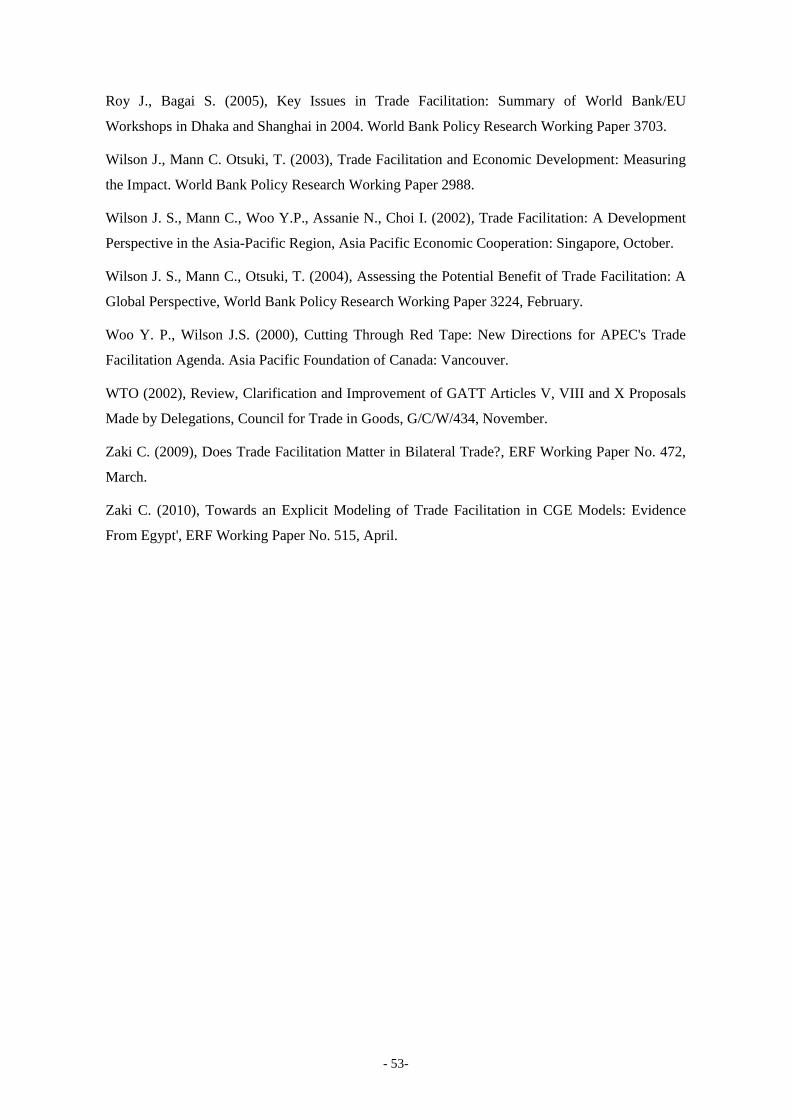
- 53-

Roy J., Bagai S. (2005), Key Issues in Trade Facilitation: Summary of World Bank/EU

Workshops in Dhaka and Shanghai in 2004. World Bank Policy Research Working Paper 3703.

Wilson J., Mann C. Otsuki, T. (2003), Trade Facilitation and Economic Development: Measuring

the Impact. World Bank Policy Research Working Paper 2988.

Wilson J. S., Mann C., Woo Y.P., Assanie N., Choi I. (2002), Trade Facilitation: A Development

Perspective in the Asia-Pacific Region, Asia Pacific Economic Cooperation: Singapore, October.

Wilson J. S., Mann C., Otsuki, T. (2004), Assessing the Potential Benefit of Trade Facilitation: A

Global Perspective, World Bank Policy Research Working Paper 3224, February.

Woo Y. P., Wilson J.S. (2000), Cutting Through Red Tape: New Directions for APEC's Trade

Facilitation Agenda. Asia Pacific Foundation of Canada: Vancouver.

WTO (2002), Review, Clarification and Improvement of GATT Articles V, VIII and X Proposals

Made by Delegations, Council for Trade in Goods, G/C/W/434, November.

Zaki C. (2009), Does Trade Facilitation Matter in Bilateral Trade?, ERF Working Paper No. 472,

March.

Zaki C. (2010), Towards an Explicit Modeling of Trade Facilitation in CGE Models: Evidence

From Egypt', ERF Working Paper No. 515, April.

- 54-

2. Appendix

A-1: regional aggregation

Region Composition

1 EU27

2 USA

3 Canada

4 Japan

5 EFTA EU27

Switzerland

Norway

Iceland

Liechtenstein

6 Australia& New Zealand

7 Korea

8 Taiwan

9 China

10 India

11 Rest of South Asia Bangladesh

Pakistan

Sri Lanka

Afghanistan

Bhutan

Maldives

Nepal

12 ASEAN

13 Mexico

14 Brazil

15 Argentina

16 Rest of Mercosur Paraguay

Uruguay

17 Rest of South America Peru

Bolivia

Equator

Colombia

Venezuela

Guyana

Suriname

18 Caribbean

19 NorthAfrica Moroco

Algeria

Tunisia

Libya

Egypt

20 Rest of Africa except South Africa

21 Rest of World Rest of Europe

Former Soviet Union

Middle East

Rest of Oceania

- 55-

A- 2: sectoralaggregation

Aggregation Code Label

s01 Cereals Paddy rice

Wheat

Cereal grains nec

Processed rice

s02 Vegetable & Fruits Vegetables. fruit. nuts

s03 Oils and Fats Oil seeds

Vegetable oils and fats

s04 Sugar Sugar cane. sugar beet

Sugar

s05 Fibers and Other crops Plant-based fibers

Crops nec

Wool. silk-worm cocoons

s06 Meat Cattle.sheep.goats.horses

Animal products nec

Meat: cattle.sheep.goats.horse

Meat products nec

s07 Dairy Raw milk

Dairy products

s08 Forestry Wood Paper

Publishing Forestry

Wood products

Paper products. publishing

s09 Fishing Fishing

s10 Primary & Petroleum products Coal

Oil

Gas

Minerals nec

Petroleum. coal products

s11 Food & Tobacco Food products nec

Beverages and tobacco products

s12 Textile Leather & Clothing Textiles

Wearing apparel

Leather products

s13 Chemicals Chemical.rubber.plastic prods

s14 Other Manufactured products Mineral products nec

Metal products

Manufactures nec

s15 Metals Ferrous metals

Metals nec

s16 Cars & Trucks Motor vehicles and parts

s17 Planes Ships Bikes Trains Transport equipment nec

s18 Electronic equipment Electronic equipment

s19 Machinery Machinery and equipment nec

s20 Other services Electricity

Gas manufacture. distribution

Water

Recreation and other services

PubAdmin/Defence/Health/Educat

Dwellings

s21 Construction Construction

s22 Trade Trade

s23 Transport Transport nec

- 56-

Appendix 3 Long run impact of central scenario on regional-sectoral value added

Table A-3 Primary and food products

Source: MIRAGE – Authors’ calculations

Note: Central scenario including agriculture, NAMA, services and trade facilitation

Table A-4 Manufactures

Source: MIRAGE – Authors’ calculations

Note: Central scenario including agriculture, NAMA, services and trade facilitation

Cereals

Vegetable

& Fruits

Oils and

Fats Sugar

Fibers and

Other crops Meat Dairy

Forestry

Wood Paper

Publishing Fishing

Primary &

Petroleum

products

Argentina 3.49 0.88 3.58 1.09 2.84 6.99 0.55 -0.05 3.46 0.07

ASEAN 0.53 1.20 1.01 2.81 1.24 0.49 3.51 -0.86 1.35 -0.62

Australia & New Zealand 6.27 2.92 2.81 2.46 4.96 6.26 24.11 0.04 1.87 0.33

Brazil 3.01 0.80 2.28 2.83 7.03 7.88 1.94 0.47 1.96 -0.45

Canada 9.41 3.43 3.22 0.11 5.82 6.69 -5.30 0.76 2.03 0.24

Caribbean 2.71 2.72 0.58 4.36 1.49 1.47 2.29 -0.34 0.08 -0.24

China 1.08 0.55 -1.52 0.64 4.54 0.17 1.02 0.00 0.19 -1.63

EFTA -19.48 -22.06 14.16 -26.43 -21.38 -43.02 -15.28 0.72 -1.14 0.60

European Union -0.49 -1.42 -4.17 -12.89 -0.66 -0.72 -1.85 0.48 -0.76 0.71

India 0.42 0.27 0.47 0.35 0.22 0.14 0.45 0.18 0.29 -0.43

Japan -8.62 -1.59 -4.73 -19.71 -2.71 -13.33 -6.49 -0.52 -1.44 0.31

Korea 1.76 -1.31 -0.18 2.14 0.72 -0.04 3.40 0.51 -3.73 3.59

Mexico 3.83 1.32 2.63 0.40 2.29 1.91 0.29 -0.01 0.40 0.71

North Africa 4.70 0.47 22.35 2.19 0.33 -1.37 3.89 -1.25 -0.19 1.62

Rest of Afr. (except Sth Afr.) 1.58 0.41 0.97 5.79 0.70 0.68 3.08 0.17 0.04 -0.48

Rest of Mercosur 3.13 0.59 1.19 0.37 1.21 1.04 0.60 -0.48 0.59 1.18

Rest of South America 2.47 5.77 1.15 3.52 2.36 1.86 3.10 -0.19 0.74 -0.15

Rest of South Asia 0.57 0.21 0.43 1.16 1.06 0.39 0.07 0.10 0.46 -0.82

Rest of World 1.53 0.01 1.18 0.82 1.44 -0.05 0.13 0.37 0.46 -0.00

Taiwan 5.09 1.01 -1.20 0.79 7.14 1.57 -0.95 0.55 -0.36 1.74

USA -8.40 2.15 -0.52 0.69 -6.32 2.33 1.07 0.41 1.73 0.65

Food &

Tobacco

Textile

Leather &

Clothing Chemicals

Other

Manufactur

ed products Metals

Cars &

Trucks

Planes Ships

Bikes Trains

Electronic

equipment Machinery

Argentina 1.69 -3.33 -3.42 -1.35 -2.95 -4.12 0.71 -0.31 -6.37

ASEAN 1.51 7.32 1.45 -0.20 -4.36 0.22 -1.59 0.08 -2.70

Australia & New Zealand 1.89 -21.50 -0.66 -0.85 -3.22 -10.41 -0.57 0.74 -3.09

Brazil 1.33 -1.38 -1.98 -1.02 -1.20 -3.62 -2.81 -1.94 -2.30

Canada -0.03 -17.17 -0.22 -0.43 0.81 -3.74 2.61 2.53 1.67

Caribbean -0.74 7.81 -0.65 -0.87 -1.64 -1.91 -2.43 -2.11 -1.13

China 0.44 5.62 0.46 0.96 0.28 -0.47 1.04 0.31 0.54

EFTA -5.65 4.82 2.18 1.33 2.76 -0.33 1.20 2.30 3.14

European Union 0.64 -2.04 0.29 0.34 -0.21 -2.05 1.29 1.78 1.03

India 0.47 -0.24 0.12 0.44 0.95 1.33 -0.12 0.50 0.30

Japan -1.23 -5.14 0.75 0.24 0.31 12.22 -2.48 -0.42 -2.55

Korea -0.41 11.05 -2.67 -0.68 -0.28 -0.64 -1.82 3.61 1.37

Mexico -0.12 -8.78 0.05 -0.36 0.58 0.33 0.31 1.26 0.66

North Africa 0.03 -6.76 -5.43 -2.07 2.56 -3.29 3.24 1.48 1.69

Rest of Afr. (except Sth Afr.) -0.12 -3.44 1.16 0.48 3.08 -0.95 1.24 -1.74 -2.48

Rest of Mercosur 0.50 -3.79 -0.74 -1.14 0.70 -0.82 1.63 1.26 -2.81

Rest of South America 0.24 -3.35 -0.33 -0.51 -3.01 -0.62 -0.65 6.22 -3.56

Rest of South Asia 0.41 1.52 0.45 0.07 -1.48 -1.40 -3.25 -1.19 -1.61

Rest of World 0.10 -1.96 -0.85 -0.13 -0.54 0.35 1.77 1.80 0.07

Taiwan -0.87 32.05 10.91 0.90 5.01 -11.21 5.96 -1.94 2.02

USA 0.55 -11.44 0.60 0.15 0.79 -0.17 0.84 2.68 1.06

- 57-

Table A-5 Services

Source: MIRAGE – Authors’ calculations

Note: Central scenario including agriculture, NAMA, services and trade facilitation

Other

services Construction Trade Transport

Communicat

ion

Financial

services

Business

services

Argentina 0.31 0.44 0.29 0.45 0.18 0.18 0.25

ASEAN 0.84 1.50 0.81 1.49 0.06 -0.03 -1.25

Australia & New Zealand 0.23 0.39 0.31 0.51 0.13 0.19 0.04

Brazil 0.17 0.30 0.18 0.48 0.04 0.03 0.17

Canada 0.16 0.13 0.14 0.65 0.18 0.24 0.14

Caribbean -0.01 0.06 0.18 0.21 -0.03 -0.04 -0.20

China 0.56 0.99 0.35 0.65 0.31 0.22 0.33

EFTA 0.98 0.87 1.01 1.98 0.62 1.01 0.67

European Union 0.27 0.27 0.38 0.99 0.29 0.37 0.30

India 0.41 0.52 0.29 0.57 0.17 0.14 -0.48

Japan 0.44 0.46 0.32 0.29 0.18 -0.03 0.07

Korea 0.59 0.79 0.46 1.44 0.35 0.33 0.17

Mexico -0.05 0.10 0.02 0.04 -0.05 0.19 -0.41

North Africa 0.15 -0.00 0.00 1.61 0.73 0.52 1.81

Rest of Afr. (except Sth Afr.) 0.70 0.85 0.50 1.55 0.56 0.44 0.81

Rest of Mercosur 0.14 0.15 0.03 -0.04 0.11 0.04 -0.06

Rest of South America 0.36 0.64 0.42 0.57 0.19 0.10 -0.12

Rest of South Asia 0.23 0.38 0.15 0.26 0.02 0.09 -0.61

Rest of World 0.19 0.26 0.20 0.66 0.26 0.22 0.41

Taiwan 1.17 1.48 0.82 1.12 0.34 0.52 -0.05

USA 0.13 0.12 0.12 0.26 0.11 0.11 0.10