Economic analyses and forecasts...task to deliver the macroeconomic forecasts that are used to set...

WORKING PAPER 12-17

Federal Planning Bureau Economic analyses and forecasts

Accuracy assessment of the FPB short-term forecasts

An update

September 2017

Ludovic Dobbelaere, [email protected] Igor Lebrun, [email protected]

Avenue des Arts 47-49 – Kunstlaan 47-49 1000 Brussels E-mail: [email protected] http://www.plan.be

National Accounts Institute

Federal Planning Bureau

The Federal Planning Bureau (FPB) is a public agency that carries out, in support of political decision-making, forecasts and studies on economic, social-economic and environmental policy issues and ex-amines their integration into a context of sustainable development. It shares its expertise with the gov-ernment, parliament, social partners, national and international institutions.

The FPB adopts an approach characterised by independence, transparency and the pursuit of the gen-eral interest. It uses high-quality data, scientific methods and empirical validation of analyses. The FPB publishes the results of its studies and, in this way, contributes to the democratic debate.

The Federal Planning Bureau is EMAS-certified and was awarded the Ecodynamic enterprise label (three stars) for its environmental policy.

Publications

Recurrent publications: Outlooks

Planning Papers (latest publication): The Planning Papers aim to diffuse the FPB’s analysis and research activities. 115 Les charges administratives en Belgique pour l’année 2014 /

De administratieve lasten in België voor het jaar 2014 Chantal Kegels, Dirk Verwerft - February 2016

Working Papers (latest publication): 11-17 Growth and Productivity in Belgium

Bernadette Biatour, Chantal Kegels - October 2017

With acknowledgement of the source, reproduction of all or part of the publication is authorised, except for commercial purposes.

Responsible publisher: Philippe Donnay Legal Deposit: D/2017/7433/29

WORKING PAPER 12-17

Federal Planning Bureau Avenue des Arts - Kunstlaan 47-49, 1000 Brussels phone: +32-2-5077311 fax: +32-2-5077373 e-mail: [email protected] http://www.plan.be

Accuracy assessment of the FPB short-term forecasts

An update

September 2017

Ludovic Dobbelaere, [email protected], Igor Lebrun, [email protected]

Abstract - The Federal Planning Bureau is responsible, within the National Accounts Institute, for pro-ducing the macroeconomic forecasts that are used to set up the federal government budget. This work-ing paper presents an update of the ex post assessment of the quality of these forecasts. Compared to the previous working paper devoted to this topic, the sample has been extended by six additional years and the number of evaluated variables has been increased, in particular with series at current prices. More-over, this paper also examines to what extent the observed forecast errors are due to errors made on exogenous assumptions related to the international environment.

Jel Classification - C53, E6 Keywords - Economic budget, Forecasts, Post-mortem assessment

WORKING PAPER 12-17

Table of contents

Executive summary ................................................................................................ 1

1. Introduction.................................................................................................... 3

2. Data description .............................................................................................. 4

2.1. Variables 4

2.2. Outcomes 4

2.3. Forecasting rounds 5

2.4. Graphical inspection of forecasts and outcomes 6

2.4.1. Real GDP and expenditure components 6

2.4.2. Consumer price index and deflator of GDP and expenditure components 8

2.4.3. Nominal GDP and income components 10

2.4.4. Labour market variables 11

3. Quality of forecasts ......................................................................................... 12

3.1. Size of forecast errors 12

3.2. Absence of bias 13

3.3. No persistence in forecast errors 14

3.4. Comparison with alternative forecasts 15

3.4.1. Comparison with naïve forecasts 15

3.4.2. Comparison with the European Commission forecasts 16

3.5. Forecast revisions 18

3.6. Directional accuracy 19

3.7. Comparison with the results of the previous study 19

4. Influence of international assumptions ................................................................. 21

4.1. Impact on GDP growth forecast errors 21

4.1.1. World trade 21

4.1.2. Interest rates 23

4.2. Impact on CPI growth forecast errors 24

5. References .................................................................................................... 25

Annex 1. Summary statistics and statistical tests .......................................................... 26

WORKING PAPER 12-17

List of tables

Table 1 Publication data of forecasts and annual national accounts ················································ 5

Table 2 Size of forecast errors (1994-2016) ············································································· 12

Table 3 Unbiasedness of forecasts (1994-2016) ········································································ 14

Table 4 Serial correlation of forecast errors (1994-2016) ···························································· 15

Table 5 Theil coefficients (1994-2016) ·················································································· 16

Table 6 Unbiasedness and independence of forecast revisions (1994-2016) ······································· 18

Table 7 Proportion of correctly predicted growth accelerations and decelerations (1994-2016) ·············· 19

Table 8 Evolution of the size of the forecast errors by adding the period 2011-2016···························· 20

Table 9 Regression results – Dependent variable: GDP growth errors (round 1 and 2) ··························· 23

List of graphs

Graph 1 Forecasts and outcomes of real GDP and expenditure components ········································ 7

Graph 2 Forecasts and outcomes of price variables ····································································· 9

Graph 3 Forecasts and outcomes of nominal GDP and income components ········································ 10

Graph 4 Forecasts and outcomes of labour market variables ························································ 11

Graph 5 Real GDP and CPI growth forecast errors: FPB vs EC Percentage points ································· 17

Graph 6 Potential export markets and export growth: forecast errors ············································· 21

Graph 7 Potential export markets and GDP growth: forecast errors (round 1 and 2) ···························· 22

Graph 8 Long-term interest rate and potential export market growth: forecast errors ························· 23

Graph 9 Imports deflator and CPI growth: forecast errors (round 1 and 2) ········································ 24

WORKING PAPER 12-17

1

Executive summary

The Federal Planning Bureau is responsible, within the National Accounts Institute, for producing the macroeconomic forecasts that are used to set up the federal government budget. According to its guid-ing principles, the FPB is as transparent as possible about its forecasts, which not only implies that a clear description of the hypotheses is available, but also of the tools and methods used to produce the forecasts. To further enhance transparency, the FPB has – at its own initiative – regularly produced ex post assessments of the quality of its forecasts in the past. Since the Law of 21 December 1994 creating the National Accounts Institute was amended by the Law of 28 February 2014, this evaluation has become mandatory and must be submitted to a scientific committee. The result of that evaluation shall also be made public and taken into account appropriately in upcoming macroeconomic forecasts.

Within this new legal framework, the present working paper provides an update of the post-mortem assessment of the annual forecasts from 2012. Compared to this previous study, the sample has been extended by six additional years and the number of evaluated variables has been increased. Moreover, this paper examines to what extent the observed forecast errors on economic growth and inflation are due to errors made on the exogenous assumptions related to the international environment.

Although several hundreds of variables are forecast in an economic budget, only the most relevant ones to set up the government budget were selected for the evaluation. Real growth in GDP and expenditure components were chosen as the most important indicators of economic activity. Analogously, growth in the consumer price index, in the GDP deflator and in the deflators of the expenditure components are the price variables that will be covered in this analysis. Growth in nominal GDP and its main income components were selected because they are crucial to accurately forecast tax bases for corporate and personal income taxes. Finally, growth in employment and unemployment were considered the most relevant indicators for the labour market. As in previous post-mortem analyses, it was decided to define the outcomes used to assess the quality of the forecasts as the first available estimates of the national accounts. Forecast errors are defined as the difference between forecasts and realisations.

The quality of the annual forecasts is evaluated for three successive forecasting rounds, namely the year-ahead forecasts in September and the current-year forecasts in February and September, with the em-phasis being put on the first two rounds. The statistical tests performed give the following results. Fore-cast errors for all variables decline as the horizon shortens, but year-ahead forecasts exhibit sizeable mean absolute errors and contain little information on the variation around the sample mean. Errors are particularly large in the case of severe economic downturns or sudden changes in inflation. The positive bias observed in first-round real GDP forecasts is nonetheless not statistically significant and disappears completely in February. However, the GDP deflator suffers from a positive bias that is sig-nificantly different from zero in all forecasting rounds, which leads to an overprediction of nominal GDP. Gross operating surplus is the income component that captures the largest part of this overesti-mation. Employment growth forecasts are on average too pessimistic in all three rounds.

Other properties of the forecast errors are also examined. We find little evidence of persistence in the forecast errors. The February forecasts undeniably outperform naïve forecasts and have an improved

WORKING PAPER 12-17

2

accuracy for economic growth and inflation compared to the European Commission autumn forecasts. Growth accelerations and decelerations are anticipated in most cases in all the rounds. Lastly, forecast revisions tend to be too smooth, but this is a typical characteristic of macroeconomic forecasts. Overall, the forecasts of most of the variables considered in this analysis display the desired properties, but fore-casts for real public consumption, the GDP deflator, the GFCF deflator and gross operating surplus clearly fall behind. Moreover, the analysis of the forecast errors in comparison with the results obtained in the previous study shows that the accuracy of the forecasts has generally improved over the last six years compared to the historical average. Yet, the reduction in the error size – in particular for the vari-ables in real terms – is partly attributable to a decline in volatility of the outcomes.

Finally, we analyse to what extent the observed forecast errors in economic growth and inflation are due to errors made on the exogenous assumptions related to the international environment. Regression analyses show that if the evolution of potential exports markets had been correctly anticipated, the av-erage absolute size of the year-ahead error on GDP growth would have been reduced by more than 60%. With a similar approach correcting CPI growth for errors made on import price developments, the mean absolute error of the year-ahead forecasts is decreased by 35%.

WORKING PAPER 12-17

3

1. Introduction

According to the Law of 21 December 1994, the National Accounts Institute (NAI) is entrusted with the task to deliver the macroeconomic forecasts that are used to set up the Belgian federal government budget and to perform budgetary control exercises. Within the NAI, the Federal Planning Bureau (FPB) is responsible for producing these forecasts, which are referred to in the law as the ‘economic budget’. According to its guiding principles, the FPB is as transparent as possible about its forecasts, which not only implies that a clear description of the hypotheses behind the forecasts is available, but also of the tools and methods used to produce the forecasts1. To further enhance transparency, the FPB has – at its own initiative – regularly produced ex post assessments of the quality of its forecasts in the past.2 Fol-lowing the European directive on requirements for budgetary frameworks of the Member States, the Law of 21 December 1994 creating the NAI was amended by the Law of 28 February 2014 stating that an evaluation of the economic forecasts must be carried out every three years and submitted to a scien-tific committee composed partly of members external to the NAI. The result of that evaluation shall be made public and taken into account appropriately in upcoming macroeconomic forecasts.

Within this new legal framework, the present working paper provides an update of the previous post-mortem analysis of the annual forecasts. Compared to this study, the sample has been extended by six additional years and the spectrum of evaluated variables has been increased in particular with GDP at current prices and its main income components. The latter are key to forecast the main macroeconomic tax bases. Moreover, this paper also examines to what extent the observed forecast errors on economic growth and inflation are due to errors made on the exogenous assumptions related to the international environment.

It should be noted that an ex post evaluation of forecast errors should not be considered the ultimate quality check of the FPB’s macroeconomic forecasts. In fact, a post-mortem analysis only examines prop-erties such as the size of the forecast errors and does not take into account other features of the forecast-ing exercises such as completeness and consistency, which are just as desirable in the framework of a government budget elaboration. Nonetheless, the aim of these post-mortem analyses is to give external users a quantification of the uncertainty surrounding the forecasts and, as now mentioned in the Law, to detect possible methodological weaknesses that need to be addressed.

This working paper is structured as follows. Section 2 reviews the economic variables to be examined, how outcomes have been chosen and provides a graphical comparison between forecasts and outcomes. Section 3 presents the results of the statistical tests gauging the quality of the forecasts for the selected variables. The closing section discusses the influence of international assumptions on GDP growth and inflation forecasts.

1 See HERTVELDT and LEBRUN (2003), DOBBELAERE et al. (2003), FPB (2006) and DE KETELBUTTER et al. (2014). 2 See FPB (1998), DOBBELAERE and HERTVELDT (2004), BOGAERT et al. (2006) and DOBBELAERE and LEBRUN (2012)

respectively.

WORKING PAPER 12-17

4

2. Data description

The first subsection discusses the variables that will be evaluated. The second one explains how out-comes have been determined, while the third one provides information regarding the timing of the economic budget. The final subsection compares forecasts and outcomes graphically for the set of se-lected variables.

Forecast errors are calculated as the difference between forecasts and realisations, implying that positive errors are associated with overestimations and negative errors with underestimations.

2.1. Variables

Although several hundreds of variables are forecasted in an economic budget, only the most relevant ones to set up the government budget will be considered in this evaluation:

– Real GDP and expenditure components were selected as the most important indicators of economic activity. Even if not all expenditure components are equally crucial for the government budget, they are all examined3 because of their importance to determine GDP in the FPB’s demand-driven fore-casting model.

– Consumer price index (CPI), the GDP deflator and the deflators of the expenditure components4 are the price variables that will be covered in this analysis. The CPI plays a key role in the Belgian economy that is characterised by a generalised automatic wage indexation5, while the deflator of the expenditure components is as important as their real growth to estimate, for example, VAT revenues.

– Nominal GDP and its main income components are crucial to accurately forecast tax bases for corporate and personal income taxes.

– Employment and unemployment are the indicators that will be used to assess the quality of labour mar-ket forecasts. These variables play a key role in estimating social benefits and social contributions.

To ensure an easy interpretation of the results, the evaluation is based on growth rates for all series.

2.2. Outcomes

Determining the outcomes for the CPI and the number of unemployed persons is straightforward as they are quickly available and not subject to revisions. For all other variables, the outcomes are taken from the national accounts that can be revised substantially over time. Consequently, the choice of the outcomes is not without importance as it can influence the properties of the forecast errors. As in the previous post-mortem analyses, forecasts are compared with the earliest estimates in the national ac-counts for the following reasons:

3 Except ‘changes in inventories’. 4 However, in the following sections we do not present the forecast errors for the private consumption deflator because their

properties are very similar to those for the CPI. 5 Although wages and social benefits are indexed on the basis of the health index (CPI corrected for the price evolution of motor

fuels, alcoholic beverages and tobacco products), the CPI is considered here to ensure international comparability.

WORKING PAPER 12-17

5

– Revisions of the national accounts are often related to methodological adjustments, which are im-possible to forecast.

– The variables in question have been forecast with the FPB’s quarterly macroeconometric model MODTRIM since 2002, thereby integrating all available data from the quarterly national accounts. This implies that the economic budget can be considered as a forecast of the first estimate of the annual national accounts.

Since the start of the quarterly national accounts in 1998, the first estimate for the year t has been pub-lished in April of the year t+1. In earlier years, the first estimate was available in June of the year t+1.

2.3. Forecasting rounds

The FPB publishes two economic budgets per year: one in September of the year t-1 that is used to set up the budget for the year t and one in February of the year t that serves as an input for the budgetary control of the year t. Until 2001, the economic budget was finalised at the beginning of July, while it has been available by September since 2002. However, the FPB has continued to produce a preliminary forecasting exercise in June of the year t-1 allowing other institutions to start their budgetary exercise for the year t so they can prepare the production of the final figures in September. These preliminary results will not be considered in this post-mortem analysis. In what follows, “September forecasts” should thus be understood as a mix of forecasts that were finalised in July (up to 2001) and September (from 2002 onwards).

Table 1 Publication data of forecasts and annual national accounts month \ year t-1 t t+1September forecast t-1 (3rd round)

forecast t (1st round)

February estimate t-1 (4th round)forecast t (2nd round)

April outcome t-1September forecast t (3rd round)

forecast t+1 (1st round)

February estimate t (4th round) forecast t+1

April outcome t

Table 1 shows that four forecasts/estimates are published in successive economic budgets before the first outcome is available. As forecast errors of the fourth-round estimate are generally very small, only the September forecasts for the year ahead (first round) and the February and September forecasts for the current year (second and third round respectively) will be discussed. As forecasts are available from 1994 onwards and observations up to 2016, 23 data points per round of forecasts can be calculated. In Section 3, the statistical properties of the errors are analysed per round. In Section 4, to analyse the influence of international assumptions, data points of the first two rounds are pooled to increase the robustness of the regression results.

WORKING PAPER 12-17

6

2.4. Graphical inspection of forecasts and outcomes

This section presents graphs with first- and second-round forecasts and outcomes for all variables. While the statistical tests presented in Section 3 translate the properties of the forecast errors into a single figure, this section provides a detailed time perspective of forecast errors that allows us to better under-stand their dynamics, including the identification of outliers.

2.4.1. Real GDP and expenditure components

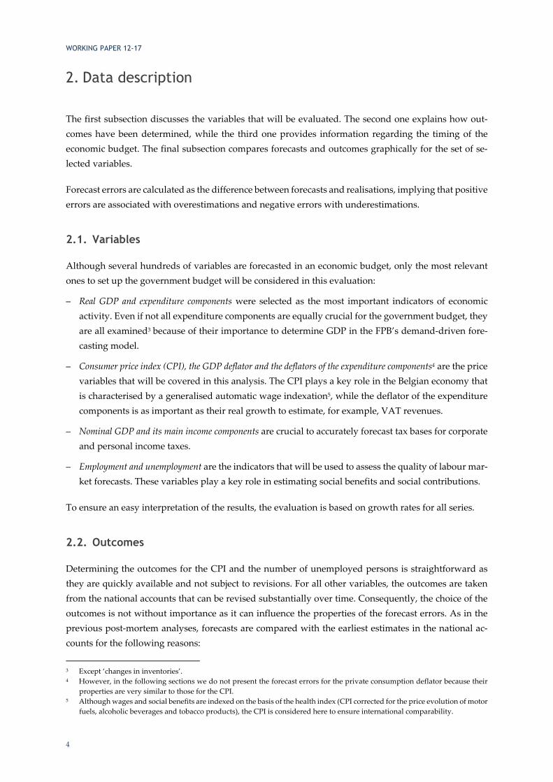
As can be seen in Graph 1, GDP growth forecast errors made in February of the current year are strongly correlated with errors made in September of the previous year: only four times (1999, 2011, 2015 and 2016) do they exhibit a different sign for a same year and in all four cases the errors in one round are close to zero. A major difference between the two forecasting rounds is the removal of the largest errors in February.6 More generally, the year-ahead forecasts appear to be much less volatile than outcomes, implying the appearance of negative forecast errors during growth accelerations and positive ones dur-ing growth decelerations. The same kind of pattern in forecast errors is to be found in private consump-tion, GFCF and export growth and, consequently, import growth. The main difference between these variables is the size of the errors: they tend to be significantly higher for volatile variables. While forecast errors for private consumption growth are only occasionally higher than 1 percentage point, those for GFCF can amount to 6 percentage points and even more for exports and imports in years characterised by a pronounced upturn or downturn.

Forecast errors on public consumption have very different characteristics as this variable is not related to the business cycle. Here we can distinguish two periods. Until 2004, public consumption growth was underestimated in both rounds with no accuracy improvement in February. From 2005 onwards, it was overestimated in most cases with a clear reduction in the forecast errors in the second round. However, these forecast errors should be interpreted with caution as forecasts related to public expenditure are based on the ‘no-policy-change’ rule. It stipulates that only fiscal measures that are known with a suffi-cient degree of detail and certainty can be included in the forecast. In other words, even if additional measures are considered likely, they cannot be incorporated as long as they are not formally decided or known with sufficient details.

6 Namely for the years 2002 (the aftermath of the dot-com bubble and the 9/11 terrorist attacks), 2009 (the global financial crisis),

2010 (the stronger than expected rebound in world trade) and 2012 (the euro area sovereign debt crisis). The year 2001 is an exception: the strong slowdown in economic activity was anticipated neither in the September nor in the February forecasts.

WORKING PAPER 12-17

7

Graph 1 Forecasts and outcomes of real GDP and expenditure components Growth rates in percent

Source: NAI, FPB.

-4

-3

-2

-1

0

1

2

3

4

5

1994 1996 1998 2000 2002 2004 2006 2008 2010 2012 2014 2016

GDP

Outcome Year-ahead (September)Current year (February)

-2

-1

0

1

2

3

4

1994 1996 1998 2000 2002 2004 2006 2008 2010 2012 2014 2016

Private consumption


-0.5

0.0

0.5

1.0

1.5

2.0

2.5

3.0

3.5

1994 1996 1998 2000 2002 2004 2006 2008 2010 2012 2014 2016

Public consumption


-6

-4

-2

0

2

4

6

8

10

1994 1996 1998 2000 2002 2004 2006 2008 2010 2012 2014 2016

Gross fixed capital formation


-15

-10

-5

0

5

10

15

1994 1996 1998 2000 2002 2004 2006 2008 2010 2012 2014 2016

Exports of goods and services


-15

-10

-5

0

5

10

15

1994 1996 1998 2000 2002 2004 2006 2008 2010 2012 2014 2016

Imports of goods and services


WORKING PAPER 12-17

8

2.4.2. Consumer price index and deflator of GDP and expenditure components

Forecasts and outcomes for the CPI, the GDP deflator and components are shown in Graph 2. Forecast revisions for CPI growth between September and February are very limited until 2005. Afterwards, the increased volatility in outcomes is clearly better reflected in the current-year forecasts. The large year- ahead forecast errors for the CPI since 2008, with both over- and underestimations, are related to ex-treme energy price developments that were better apprehended in the February edition of the economic budget. The evolution of the GDP deflator is clearly overestimated in both forecasting rounds during the second half of the 1990s and since 2007 with a particularly large error in 2009. Current-year forecasts have been more accurate than year-ahead forecasts since 2010.

The growth rate of the deflator of public consumption was overestimated in both rounds at the begin-ning of the sample and has been almost systematically underestimated since 1999 with the notable ex-ception of 2009. The largest errors over the two forecasting rounds occur in the years 1996, 2008 and 2009. The evolution of the deflator of gross fixed capital formation is overestimated 18 times in Septem-ber and 15 times in February. Again, the largest error appears in 2009. The export and import deflators are extremely volatile and consequently difficult to forecast accurately.7 Very large errors show up in both rounds for the years 2000 and 2005 and during the 2008-2011 period.

7 Moreover, exports and imports deflators are also subject to large statistical revisions.

WORKING PAPER 12-17

9

Graph 2 Forecasts and outcomes of price variables Growth rates in percent

Source: NAI, FPS Economy, FPB.

-1

0

1

2

3

4

5

1994 1996 1998 2000 2002 2004 2006 2008 2010 2012 2014 2016

Consumer price index


0.0

0.5

1.0

1.5

2.0

2.5

3.0

3.5

1994 1996 1998 2000 2002 2004 2006 2008 2010 2012 2014 2016

GDP deflator


0

1

2

3

4

5

1994 1996 1998 2000 2002 2004 2006 2008 2010 2012 2014 2016

Public consumption deflator


-4

-3

-2

-1

0

1

2

3

4

1994 1996 1998 2000 2002 2004 2006 2008 2010 2012 2014 2016

GFCF deflator


-8

-6

-4

-2

0

2

4

6

8

10

12

1994 1996 1998 2000 2002 2004 2006 2008 2010 2012 2014 2016

Exports deflator


-8

-6

-4

-2

0

2

4

6

8

10

12

1994 1996 1998 2000 2002 2004 2006 2008 2010 2012 2014 2016

Imports deflator


WORKING PAPER 12-17

10

2.4.3. Nominal GDP and income components

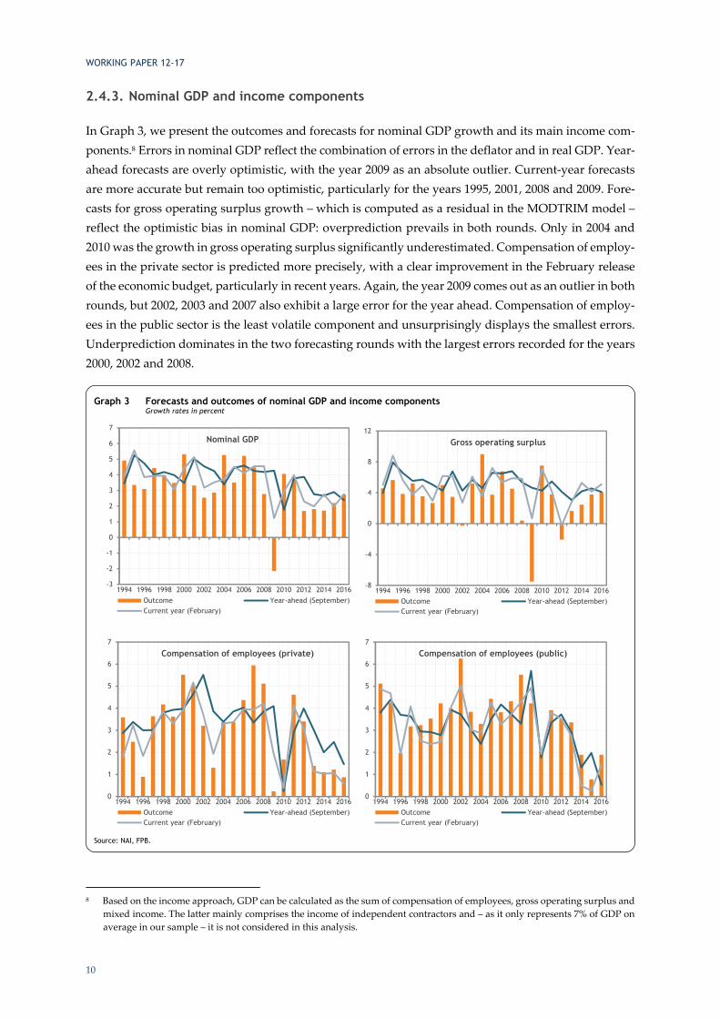
In Graph 3, we present the outcomes and forecasts for nominal GDP growth and its main income com-ponents.8 Errors in nominal GDP reflect the combination of errors in the deflator and in real GDP. Year-ahead forecasts are overly optimistic, with the year 2009 as an absolute outlier. Current-year forecasts are more accurate but remain too optimistic, particularly for the years 1995, 2001, 2008 and 2009. Fore-casts for gross operating surplus growth – which is computed as a residual in the MODTRIM model – reflect the optimistic bias in nominal GDP: overprediction prevails in both rounds. Only in 2004 and 2010 was the growth in gross operating surplus significantly underestimated. Compensation of employ-ees in the private sector is predicted more precisely, with a clear improvement in the February release of the economic budget, particularly in recent years. Again, the year 2009 comes out as an outlier in both rounds, but 2002, 2003 and 2007 also exhibit a large error for the year ahead. Compensation of employ-ees in the public sector is the least volatile component and unsurprisingly displays the smallest errors. Underprediction dominates in the two forecasting rounds with the largest errors recorded for the years 2000, 2002 and 2008.

8 Based on the income approach, GDP can be calculated as the sum of compensation of employees, gross operating surplus and

mixed income. The latter mainly comprises the income of independent contractors and – as it only represents 7% of GDP on average in our sample – it is not considered in this analysis.

Graph 3 Forecasts and outcomes of nominal GDP and income components Growth rates in percent

Source: NAI, FPB.

-3

-2

-1

0

1

2

3

4

5

6

7

1994 1996 1998 2000 2002 2004 2006 2008 2010 2012 2014 2016

Nominal GDP


-8

-4

0

4

8

12

1994 1996 1998 2000 2002 2004 2006 2008 2010 2012 2014 2016

Gross operating surplus


0

1

2

3

4

5

6

7

1994 1996 1998 2000 2002 2004 2006 2008 2010 2012 2014 2016

Compensation of employees (private)


0

1

2

3

4

5

6

7

1994 1996 1998 2000 2002 2004 2006 2008 2010 2012 2014 2016

Compensation of employees (public)


WORKING PAPER 12-17

11

2.4.4. Labour market variables

When assessing forecasts for the number of employed and unemployed persons, it should be kept in mind that the magnitude of the growth rates of both variables cannot be compared since 1% of employ-ment represented 46 000 persons in 2015, while 1% of unemployment only amounted to around 6 000 persons. Consequently, forecast errors expressed in percentage points will be larger for unemployment than for employment.

Overall, underpredictions of employment go hand in hand with overpredictions of unemployment and vice-versa. This implies that forecast errors for the labour force are generally smaller than those for employment. Year-ahead forecasts for employment growth are overly optimistic for the period 2001-2003, but during the 2004-2011 period employment growth was underestimated each year, with the notable exception of 2009. The February forecasts are more accurate, especially at the beginning of the 2000s and for the years 2009 and 2011. Unsurprisingly, unemployment forecasts also generally improve between the economic budget of September and of February, with notable exceptions for the years 1995 and 2015.

Graph 4 Forecasts and outcomes of labour market variables Growth rates in percent

Source: NAI, RVA/ONEM, FPB.

-1.5

-1.0

-0.5

0.0

0.5

1.0

1.5

2.0

1994 1996 1998 2000 2002 2004 2006 2008 2010 2012 2014 2016

Employment


-12

-8

-4

0

4

8

12

16

1994 1996 1998 2000 2002 2004 2006 2008 2010 2012 2014 2016

Unemployment


WORKING PAPER 12-17

12

3. Quality of forecasts

The quality of the FPB forecasts will be evaluated based on several criteria. The mathematical formulas that are used to calculate the indicators as well as the formalisation of the statistical tests can be found in Annex 1. Note that the methods applied below are those traditionally used by international organi-sations such as the EC, the OECD and the IMF to assess the accuracy of their own forecasts. 9 As in the previous section, the sample covers the 1994-2016 period.

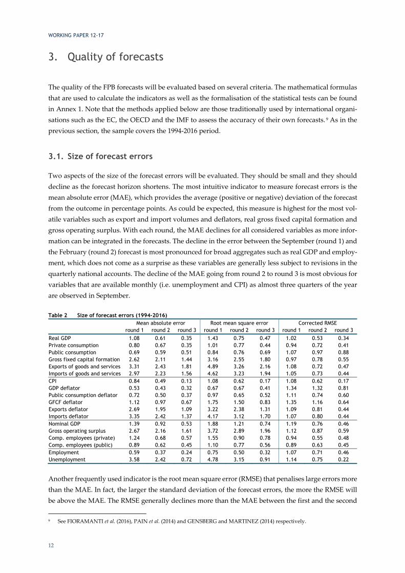
3.1. Size of forecast errors

Two aspects of the size of the forecast errors will be evaluated. They should be small and they should decline as the forecast horizon shortens. The most intuitive indicator to measure forecast errors is the mean absolute error (MAE), which provides the average (positive or negative) deviation of the forecast from the outcome in percentage points. As could be expected, this measure is highest for the most vol-atile variables such as export and import volumes and deflators, real gross fixed capital formation and gross operating surplus. With each round, the MAE declines for all considered variables as more infor-mation can be integrated in the forecasts. The decline in the error between the September (round 1) and the February (round 2) forecast is most pronounced for broad aggregates such as real GDP and employ-ment, which does not come as a surprise as these variables are generally less subject to revisions in the quarterly national accounts. The decline of the MAE going from round 2 to round 3 is most obvious for variables that are available monthly (i.e. unemployment and CPI) as almost three quarters of the year are observed in September.

Table 2 Size of forecast errors (1994-2016) Mean absolute error Root mean square error Corrected RMSE round 1 round 2 round 3 round 1 round 2 round 3 round 1 round 2 round 3

Real GDP 1.08 0.61 0.35 1.43 0.75 0.47 1.02 0.53 0.34Private consumption 0.80 0.67 0.35 1.01 0.77 0.44 0.94 0.72 0.41Public consumption 0.69 0.59 0.51 0.84 0.76 0.69 1.07 0.97 0.88Gross fixed capital formation 2.62 2.11 1.44 3.16 2.55 1.80 0.97 0.78 0.55Exports of goods and services 3.31 2.43 1.81 4.89 3.26 2.16 1.08 0.72 0.47Imports of goods and services 2.97 2.23 1.56 4.62 3.23 1.94 1.05 0.73 0.44CPI 0.84 0.49 0.13 1.08 0.62 0.17 1.08 0.62 0.17GDP deflator 0.53 0.43 0.32 0.67 0.67 0.41 1.34 1.32 0.81Public consumption deflator 0.72 0.50 0.37 0.97 0.65 0.52 1.11 0.74 0.60GFCF deflator 1.12 0.97 0.67 1.75 1.50 0.83 1.35 1.16 0.64Exports deflator 2.69 1.95 1.09 3.22 2.38 1.31 1.09 0.81 0.44Imports deflator 3.35 2.42 1.37 4.17 3.12 1.70 1.07 0.80 0.44Nominal GDP 1.39 0.92 0.53 1.88 1.21 0.74 1.19 0.76 0.46Gross operating surplus 2.67 2.16 1.61 3.72 2.89 1.96 1.12 0.87 0.59Comp. employees (private) 1.24 0.68 0.57 1.55 0.90 0.78 0.94 0.55 0.48Comp. employees (public) 0.89 0.62 0.45 1.10 0.77 0.56 0.89 0.63 0.45Employment 0.59 0.37 0.24 0.75 0.50 0.32 1.07 0.71 0.46Unemployment 3.58 2.42 0.72 4.78 3.15 0.91 1.14 0.75 0.22

Another frequently used indicator is the root mean square error (RMSE) that penalises large errors more than the MAE. In fact, the larger the standard deviation of the forecast errors, the more the RMSE will be above the MAE. The RMSE generally declines more than the MAE between the first and the second

9 See FIORAMANTI et al. (2016), PAIN et al. (2014) and GENSBERG and MARTINEZ (2014) respectively.

WORKING PAPER 12-17

13

forecasting round, which not only indicates that forecast errors are smaller in February than in Septem-ber, but also that large errors are less common in February. The forecasts for the GDP deflator are an exception to this rule.

To adjust for the fact that volatile series are generally accompanied by large forecast errors, a corrected RMSE was calculated by dividing the RMSE by the standard deviation of the series. This brings the values of the indicator much closer to each other in all forecasting rounds. Only forecasts for public consumption and for the GDP and GFCF deflators seem to perform much worse than the other ones. Another property of this indicator is that it will be smaller than one if the FPB forecasts are more accu-rate than the alternative forecast corresponding to the full sample average of the variable.10 The cor-rected RMSE is close to or above one for all variables in the first round, i.e. the forecasts contain little information on the variation around the sample mean. From the second forecasting round onwards, FPB forecasts perform much better than average forecasts, except again for real public consumption and for the GDP and the GFCF deflators. The comparisons with alternative forecasts will be discussed more extensively in subsection 3.4.

3.2. Absence of bias

Irrespective of the size of the errors, forecasts should be unbiased. In other words, they should not be systematically too optimistic or too pessimistic, implying that positive and negative forecast errors should offset each other on average. The presence of a bias suggests that forecast accuracy can be im-proved using this information.

A first indication can be provided by the percentage of positive forecast errors, which should be close to 50% in the case of unbiased forecasts. Table 3 shows that this is the case in first and second round forecasts for real GDP and components. However, overpredictions are dominant for forecasts on the GFCF deflator and gross operating surplus, while underpredictions prevail for compensation of public sector employees and employment.

To test whether the bias is statistically significant, forecast errors were regressed on a constant. The estimated constant of this equation is equal to the mean error (ME). It is positive for real GDP and all expenditure components – except public consumption – in the year-ahead forecasts, although not sig-nificantly different from zero. It should be noted that the positive ME for real GDP is mainly related to the outlier in the forecast errors in 2009. If that particular year is left out of the sample, the ME falls to 0.16 for real GDP growth, becomes virtually zero for private consumption and even slightly negative for GFCF. The influence of this outlier disappears from the second forecasting round onwards, bringing the ME very close to zero for GDP and private consumption and into negative territory for GFCF. The ME remains negative for public consumption growth and is significantly different from zero in round 2. The ME for export and import growth is much closer to zero in round 2 and even becomes signifi-cantly negative in the third round.

10 As can be easily deduced from the mathematical formulas presented in Annex 1, the standard deviation of a variable corre-

sponds to the RMSE if every forecast is equal to the sample average of that variable. Note that in practice it is impossible to use the whole sample average as a forecast because it is unknown at the time the forecast is produced.

WORKING PAPER 12-17

14

Table 3 Unbiasedness of forecasts (1994-2016) Percentage of positive forecast errors Mean error round 1 round 2 round 3 round 1 round 2 round 3

Real GDP 61 52 39 0.34 -0.02 -0.06Private consumption 52 57 39 0.13 -0.01 -0.00Public consumption 48 43 48 -0.13 -0.29* -0.16Gross fixed capital formation 43 48 65 0.17 -0.32 0.03Exports of goods and services 57 52 43 1.01 0.29 -0.87**Imports of goods and services 52 48 30 0.71 0.19 -0.86**CPI 52 30 57 -0.06 -0.21 0.02GDP deflator 61 78 74 0.25* 0.35** 0.17**Public consumption deflator 43 39 61 0.04 -0.06 0.08GFCF deflator 78 65 65 0.95** 0.59** 0.37**Exports deflator 52 52 57 -0.09 -0.31 0.10Imports deflator 48 52 52 -0.18 -0.74 -0.04Nominal GDP 61 61 57 0.60** 0.33 0.11Gross operating surplus 78 83 78 1.87** 1.40** 0.83**Comp. employees (private) 57 30 43 0.28 -0.27* -0.29**Comp. employees (public) 30 22 30 -0.40* -0.43** -0.24**Employment 35 22 17 -0.14 -0.28** -0.13**Unemployment 52 65 70 0.58 1.27 0.20Note: * and ** denote that the mean error is significantly different from zero at the 10 % and the 5 % level respectively. Significance levels were

calculated based on standard errors robust to autocorrelation and heteroskedasticity.

CPI forecast errors register a negative bias in the second round that is close to being statistically signif-icant at a 10% level. The GDP deflator suffers from a positive bias that is significantly different from zero in all forecasting rounds. This overprediction is also present in the GFCF deflator forecasts. The ME is negative, but not significantly different from zero, for the exports and imports deflators in round 1 and 2.

Nominal GDP growth is overpredicted in all rounds and the bias is significant in round 1. The ME for gross operating surplus is also positive and significantly different from zero in the three rounds. The growth in compensation of employees is underestimated in all rounds, except for the private sector in the first round. The ME for employment is negative in all rounds and significantly different from zero in round 2 and 3. That is mirrored in positive forecast errors for unemployment. Considering the ME for both real GDP and employment growth, one can also infer that productivity growth has been over-estimated substantially in the first two rounds.

3.3. No persistence in forecast errors

Next to the significance of the forecast bias, the equations estimated in subsection 3.2 also allow us to check for serial correlation in forecast errors. The presence of serial correlation implies that past forecast errors could be used to improve the forecast in year t. First- and second-order correlation coefficients are reported in Table 4. Positive values imply that the forecasters repeat the same mistakes, negative ones that they compensate past mistakes by subsequent errors of the opposite sign.

WORKING PAPER 12-17

15

Table 4 Serial correlation of forecast errors (1994-2016) 1st order serial correlation 2nd order serial correlation round 1 round 2 round 3 round 1 round 2 round 3

Real GDP -0.14 -0.25 -0.09 -0.32 -0.22 -0.24Private consumption 0.01 -0.15 0.27 -0.20 -0.24 -0.07Public consumption 0.55** 0.23 0.24 0.26** 0.15 0.15Gross fixed capital formation 0.13 0.45** 0.30 -0.21 0.04* -0.04Exports of goods and services -0.21 -0.17 -0.09 -0.19 -0.05 -0.40*Imports of goods and services -0.21 -0.19 -0.04 -0.21 -0.08 -0.31CPI -0.15 0.05 0.01 -0.29 -0.03 -0.14GDP deflator 0.11 0.11 -0.09 0.03 -0.06 -0.21Public consumption deflator 0.08 -0.04 -0.11 0.06 0.23 0.27GFCF deflator 0.01 -0.20 -0.33* -0.26 -0.13 0.01Exports deflator -0.02 0.09 -0.23 -0.32 -0.22 -0.44**Imports deflator -0.08 -0.01 -0.21 -0.30 -0.25 -0.61**Nominal GDP -0.21 -0.15 -0.13 -0.31 -0.19 0.23Gross operating surplus -0.12 -0.02 -0.04 -0.25 -0.16 -0.05Comp. employees (private) 0.05 -0.10 -0.17 -0.44* -0.36 -0.01Comp. employees (public) -0.09 0.12 0.15 -0.03 0.06 -0.27Employment 0.13 0.20 -0.03 -0.31 -0.08 -0.09Unemployment 0.31 0.50** -0.12 -0.02 0.28** 0.09Note: * and ** denote that the null hypothesis of no serial correlation is rejected at the 10% or the 5% level respectively. The hypothesis is tested

on the basis of the Ljung-Box Q-statistic.

Only few forecast errors suffer from serial correlation. During the first two forecasting rounds, statisti-cally significant first- or second-order autocorrelation is only seen in the forecast errors of public con-sumption, GFCF, compensation of private employees and unemployment. Serial correlation is found in the third-round forecast errors for exports and the deflators of GFCF, exports and imports.

3.4. Comparison with alternative forecasts

The forecasts can also be evaluated by comparing them with those produced with alternative methods or by other institutions.

3.4.1. Comparison with naïve forecasts

Here we want to check whether model-based forecasts using all the information available – such as the forecasts contained in the economic budget – outperform those produced with naïve methods. As we already discussed in subsection 3.1, using the sample mean of realisations as a forecasting rule is not a viable option because the sample mean is not known at the time of the forecast. At best, the forecaster could use the mean of the outcomes up to the day of the forecast. Therefore, we use the average growth rate of the 10 years prior to the forecasting exercise as a naïve alternative for extrapolation. Another rule-of-thumb method consists in simply taking the growth rate of the observation for the last available year. 11 The comparison with naïve forecasts usually relies on the Theil coefficient, which is computed as the ratio between the RMSE of the economic budget forecast and the RMSE based on the naïve ap-proach. A Theil coefficient below unity indicates that the economic budget outperforms the naïve method.

Table 5 provides the results based on the last year observed (Theil 1) and on the 10-year moving average (Theil 2). 11 This means that for round 1, the realization of the year t-1 is used to predict t+1, for round 2 the same outcome is used, while

for round 3, the outcome of the previous year can be used.

WORKING PAPER 12-17

16

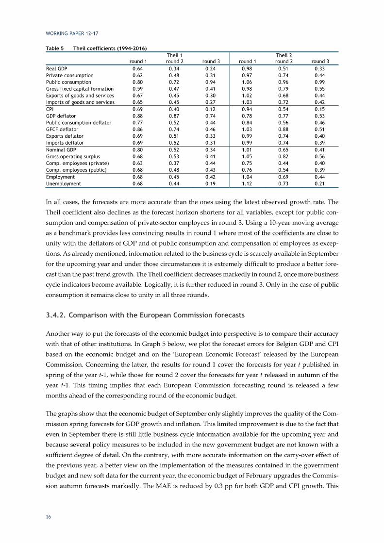
Table 5 Theil coefficients (1994-2016) Theil 1 Theil 2 round 1 round 2 round 3 round 1 round 2 round 3

Real GDP 0.64 0.34 0.24 0.98 0.51 0.33Private consumption 0.62 0.48 0.31 0.97 0.74 0.44Public consumption 0.80 0.72 0.94 1.06 0.96 0.99Gross fixed capital formation 0.59 0.47 0.41 0.98 0.79 0.55Exports of goods and services 0.67 0.45 0.30 1.02 0.68 0.44Imports of goods and services 0.65 0.45 0.27 1.03 0.72 0.42CPI 0.69 0.40 0.12 0.94 0.54 0.15GDP deflator 0.88 0.87 0.74 0.78 0.77 0.53Public consumption deflator 0.77 0.52 0.44 0.84 0.56 0.46GFCF deflator 0.86 0.74 0.46 1.03 0.88 0.51Exports deflator 0.69 0.51 0.33 0.99 0.74 0.40Imports deflator 0.69 0.52 0.31 0.99 0.74 0.39Nominal GDP 0.80 0.52 0.34 1.01 0.65 0.41Gross operating surplus 0.68 0.53 0.41 1.05 0.82 0.56Comp. employees (private) 0.63 0.37 0.44 0.75 0.44 0.40Comp. employees (public) 0.68 0.48 0.43 0.76 0.54 0.39Employment 0.68 0.45 0.42 1.04 0.69 0.44Unemployment 0.68 0.44 0.19 1.12 0.73 0.21

In all cases, the forecasts are more accurate than the ones using the latest observed growth rate. The Theil coefficient also declines as the forecast horizon shortens for all variables, except for public con-sumption and compensation of private-sector employees in round 3. Using a 10-year moving average as a benchmark provides less convincing results in round 1 where most of the coefficients are close to unity with the deflators of GDP and of public consumption and compensation of employees as excep-tions. As already mentioned, information related to the business cycle is scarcely available in September for the upcoming year and under those circumstances it is extremely difficult to produce a better fore-cast than the past trend growth. The Theil coefficient decreases markedly in round 2, once more business cycle indicators become available. Logically, it is further reduced in round 3. Only in the case of public consumption it remains close to unity in all three rounds.

3.4.2. Comparison with the European Commission forecasts

Another way to put the forecasts of the economic budget into perspective is to compare their accuracy with that of other institutions. In Graph 5 below, we plot the forecast errors for Belgian GDP and CPI based on the economic budget and on the ‘European Economic Forecast’ released by the European Commission. Concerning the latter, the results for round 1 cover the forecasts for year t published in spring of the year t-1, while those for round 2 cover the forecasts for year t released in autumn of the year t-1. This timing implies that each European Commission forecasting round is released a few months ahead of the corresponding round of the economic budget.

The graphs show that the economic budget of September only slightly improves the quality of the Com-mission spring forecasts for GDP growth and inflation. This limited improvement is due to the fact that even in September there is still little business cycle information available for the upcoming year and because several policy measures to be included in the new government budget are not known with a sufficient degree of detail. On the contrary, with more accurate information on the carry-over effect of the previous year, a better view on the implementation of the measures contained in the government budget and new soft data for the current year, the economic budget of February upgrades the Commis-sion autumn forecasts markedly. The MAE is reduced by 0.3 pp for both GDP and CPI growth. This

WORKING PAPER 12-17

17

shows the utility of the economic budget, keeping in mind that in addition it provides a more detailed forecast for the Belgian economy.

In terms of mean errors, the EC forecasts for real GDP growth exhibit an optimistic bias in round 1 that is larger than the one based on the FPB forecasts (0.6 pp against 0.4 pp). This bias remains positive in round 2 in the case of the EC (0.3 pp), while it is virtually zero for the economic budget. For inflation forecasts, the mean error in round 1 is around -0.1 pp for both institutions. In round 2, the negative bias is further reduced with the EC, while it becomes larger in the case of the FPB.

Graph 5 Real GDP and CPI growth forecast errors: FPB vs EC Percentage points

Source: NAI, FPS Economy, EC, FPB.

-3

-2

-1

0

1

2

3

4

5

1995 1998 2001 2004 2007 2010 2013 2016

Real GDP growth round 1

EC FPB

-2

-1

0

1

2

3

4

1995 1998 2001 2004 2007 2010 2013 2016

Real GDP growth round 2

EC FPB

-3

-2

-1

0

1

2

3

1995 1998 2001 2004 2007 2010 2013 2016

CPI growth round 1

EC FPB

-3

-2

-1

0

1

2

3

1995 1998 2001 2004 2007 2010 2013 2016

CPI growth round 2

EC FPB

WORKING PAPER 12-17

18

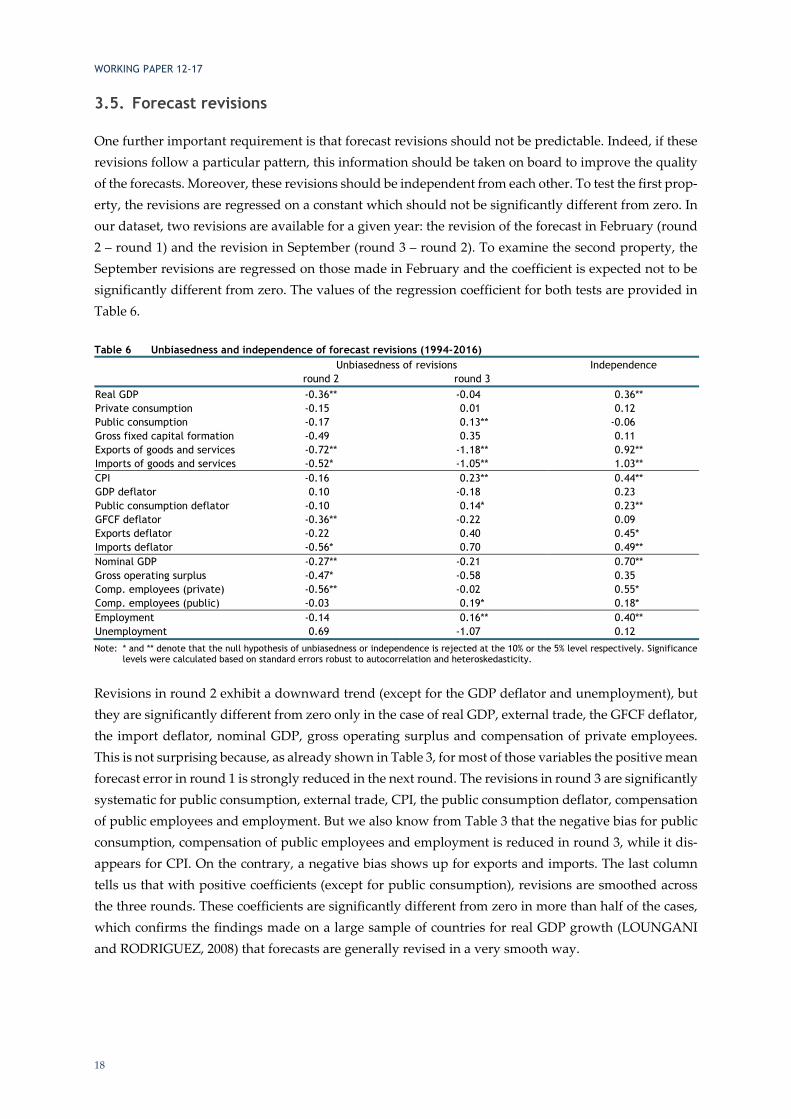
3.5. Forecast revisions

One further important requirement is that forecast revisions should not be predictable. Indeed, if these revisions follow a particular pattern, this information should be taken on board to improve the quality of the forecasts. Moreover, these revisions should be independent from each other. To test the first prop-erty, the revisions are regressed on a constant which should not be significantly different from zero. In our dataset, two revisions are available for a given year: the revision of the forecast in February (round 2 – round 1) and the revision in September (round 3 – round 2). To examine the second property, the September revisions are regressed on those made in February and the coefficient is expected not to be significantly different from zero. The values of the regression coefficient for both tests are provided in Table 6.

Table 6 Unbiasedness and independence of forecast revisions (1994-2016) Unbiasedness of revisions Independence round 2 round 3

Real GDP -0.36** -0.04 0.36** Private consumption -0.15 0.01 0.12 Public consumption -0.17 0.13** -0.06 Gross fixed capital formation -0.49 0.35 0.11 Exports of goods and services -0.72** -1.18** 0.92** Imports of goods and services -0.52* -1.05** 1.03** CPI -0.16 0.23** 0.44** GDP deflator 0.10 -0.18 0.23 Public consumption deflator -0.10 0.14* 0.23** GFCF deflator -0.36** -0.22 0.09 Exports deflator -0.22 0.40 0.45* Imports deflator -0.56* 0.70 0.49** Nominal GDP -0.27** -0.21 0.70** Gross operating surplus -0.47* -0.58 0.35 Comp. employees (private) -0.56** -0.02 0.55* Comp. employees (public) -0.03 0.19* 0.18* Employment -0.14 0.16** 0.40** Unemployment 0.69 -1.07 0.12 Note: * and ** denote that the null hypothesis of unbiasedness or independence is rejected at the 10% or the 5% level respectively. Significance

levels were calculated based on standard errors robust to autocorrelation and heteroskedasticity.

Revisions in round 2 exhibit a downward trend (except for the GDP deflator and unemployment), but they are significantly different from zero only in the case of real GDP, external trade, the GFCF deflator, the import deflator, nominal GDP, gross operating surplus and compensation of private employees. This is not surprising because, as already shown in Table 3, for most of those variables the positive mean forecast error in round 1 is strongly reduced in the next round. The revisions in round 3 are significantly systematic for public consumption, external trade, CPI, the public consumption deflator, compensation of public employees and employment. But we also know from Table 3 that the negative bias for public consumption, compensation of public employees and employment is reduced in round 3, while it dis-appears for CPI. On the contrary, a negative bias shows up for exports and imports. The last column tells us that with positive coefficients (except for public consumption), revisions are smoothed across the three rounds. These coefficients are significantly different from zero in more than half of the cases, which confirms the findings made on a large sample of countries for real GDP growth (LOUNGANI and RODRIGUEZ, 2008) that forecasts are generally revised in a very smooth way.

WORKING PAPER 12-17

19

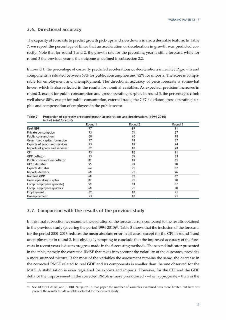
3.6. Directional accuracy

The capacity of forecasts to predict growth pick-ups and slowdowns is also a desirable feature. In Table 7, we report the percentage of times that an acceleration or deceleration in growth was predicted cor-rectly. Note that for round 1 and 2, the growth rate for the preceding year is still a forecast, while for round 3 the previous year is the outcome as defined in subsection 2.2.

In round 1, the percentage of correctly predicted accelerations or decelerations in real GDP growth and components is situated between 68% for public consumption and 82% for imports. The score is compa-rable for employment and unemployment. The directional accuracy of price forecasts is somewhat lower, which is also reflected in the results for nominal variables. As expected, precision increases in round 2, except for public consumption and gross operating surplus. In round 3, the percentages climb well above 80%, except for public consumption, external trade, the GFCF deflator, gross operating sur-plus and compensation of employees in the public sector.

Table 7 Proportion of correctly predicted growth accelerations and decelerations (1994-2016) In % of total forecasts

Round 1 Round 2 Round 3 Real GDP 77 87 91 Private consumption 73 74 87 Public consumption 68 65 78 Gross fixed capital formation 77 91 87 Exports of goods and services 73 87 74 Imports of goods and services 82 83 78 CPI 73 86 91 GDP deflator 73 74 83 Public consumption deflator 82 87 83 GFCF deflator 55 74 70 Exports deflator 64 70 87 Imports deflator 68 78 96 Nominal GDP 68 78 87 Gross operating surplus 82 78 78 Comp. employees (private) 59 91 87 Comp. employees (public) 68 70 78 Employment 82 83 91 Unemployment 73 83 91

3.7. Comparison with the results of the previous study

In this final subsection we examine the evolution of the forecast errors compared to the results obtained in the previous study (covering the period 1994-2010)12. Table 8 shows that the inclusion of the forecasts for the period 2001-2016 reduces the mean absolute error in all cases, except for the CPI in round 1 and unemployment in round 2. It is obviously tempting to conclude that the improved accuracy of the fore-casts in recent years is due to progress made in the forecasting methods. The second indicator presented in the table, namely the corrected RMSE that takes into account the volatility of the outcomes, provides a more nuanced picture. If for most of the variables the assessment remains the same, the decrease in the corrected RMSE related to real GDP and its components is smaller than the one observed for the MAE. A stabilisation is even registered for exports and imports. However, for the CPI and the GDP deflator the improvement in the corrected RMSE is more pronounced - when appropriate – than in the 12 See DOBBELAERE and LEBRUN, op. cit. In that paper the number of variables examined was more limited but here we

present the results for all variables selected for the current study.

WORKING PAPER 12-17

20

MAE. For the employment forecasts a small deterioration in round 1 is now recorded. The cross-reading of these two statistics consequently shows that the accuracy of the forecasts has been improved over the last six years compared to the historical mean, but that the reduction in the size of the errors – in partic-ular for the variables in real terms – is partly attributable to the decrease in volatility of the outcomes.

Table 8 Evolution of the size of the forecast errors by adding the period 2011-2016 Mean absolute error Corrected RMSE

round 1 round2 round 1 round 2 1994-2010 1994-2016 1994-2010 1994-2016 1994-2010 1994-2016 1994-2010 1994-2016

Real GDP 1.29 1.08 0.76 0.61 1.06 1.02 0.57 0.53Private consumption 0.89 0.80 0.77 0.67 0.96 0.94 0.76 0.72Public consumption 0.76 0.69 0.69 0.59 1.37 1.07 1.27 0.97Gross fixed capital formation 2.67 2.62 2.15 2.11 0.95 0.97 0.75 0.78Exports of goods and services 4.04 3.31 2.95 2.43 1.08 1.08 0.72 0.72Imports of goods and services 3.43 2.97 2.61 2.23 1.05 1.05 0.73 0.73CPI 0.81 0.84 0.50 0.49 1.20 1.08 0.71 0.62GDP deflator 0.55 0.53 0.51 0.43 1.50 1.34 1.57 1.32Public consumption deflator 0.82 0.72 0.54 0.50 1.23 1.11 0.81 0.74GFCF deflator 1.21 1.12 1.12 0.97 1.38 1.35 1.22 1.16Exports deflator 2.81 2.69 2.09 1.95 1.14 1.09 0.85 0.81Imports deflator 3.46 3.35 2.69 2.42 1.12 1.07 0.87 0.80Nominal GDP 1.58 1.39 1.11 0.92 1.25 1.19 0.82 0.76Gross operating surplus 2.91 2.67 2.46 2.16 1.12 1.12 0.90 0.87Comp. employees (private) 1.29 1.24 0.83 0.68 1.04 0.94 0.65 0.55Comp. employees (public) 0.95 0.89 0.65 0.62 1.12 0.89 0.76 0.63Employment 0.61 0.59 0.38 0.37 1.05 1.07 0.71 0.71Unemployment 3.81 3.58 2.15 2.42 1.16 1.14 0.65 0.75

WORKING PAPER 12-17

21

4. Influence of international assumptions

Another issue to examine is to what extent the observed forecast errors are due to errors made on the exogenous assumptions related to the international environment. To compute the developments in world trade and international prices relevant for Belgium. the economic budget relies on the forecasts produced by international organisations. The evolution of financial variables such as exchange rates and interest rates is based on market expectations or technical assumptions. The exogeneity of these variables in the forecasting process is of course related to the fact that a small economy like Belgium has a relatively insignificant impact on the world economy.

4.1. Impact on GDP growth forecast errors

4.1.1. World trade

The development of foreign export markets is a crucial exogenous variable for forecasting Belgian eco-nomic growth. The export markets hypothesis is calculated as a weighted average13 of import growth forecasts for trading partners that are primarily based on figures of the European Commission and Con-sensus Economics. 14 The left-hand panel in Graph 6 shows that export market growth forecast errors for the year ahead were extremely high in the years 2009-2010 but also in the early 2000s. Those large errors are significantly reduced in round 2.

The regression line in the right-hand panel shows the almost one-to-one relationship between the fore-cast errors made on export market and export growth.15 The goodness of fit is also remarkable as all

13 Reflecting the geographical orientation of Belgian exports. 14 The FPB relies in principle on the most recent European Commission forecasts which also serve as the reference in the budg-

etary surveillance process. However, to take into account the events occurring between the cut-off date of the Commission forecasts and the preparation of the economic budget, the Commission forecasts are updated with the latest Consensus Eco-nomics forecasts.

15 The year-ahead and current-year forecast errors have been pooled here to increase the robustness of regression.

Graph 6 Potential export markets and export growth: forecast errors Percentage points

Source: Federal Planning Bureau.

-12

-8

-4

0

4

8

12

16

1994 1996 1998 2000 2002 2004 2006 2008 2010 2012 2014 2016

Potential export markets

Year-ahead (September) Current year (February)

y = 0.96xR² = 0.85

-15

-10

-5

0

5

10

15

20

-15 -10 -5 0 5 10 15 20

Expo

rt g

row

th

Potential export market growth

Round 1 and 2

WORKING PAPER 12-17

22

data points are close to the regression line, explaining the high R-squared statistic. Correcting export growth forecasts for errors made on potential export market growth using this unitary elasticity reduces the absolute forecast error by around 60% in round 1 and by 50% in round 2. Moreover, the errors for the years 2000, 2009 and 2010 do not appear as outliers anymore.

Next to the direct impact on exports, international trade shocks also have an indirect impact on the other expenditure components. The positive slope of the regression line in Graph 7 shows the clear relation-ship between the errors on foreign export market growth and on Belgian GDP growth. The estimated coefficient indicates that for each percentage point error on export market growth, the GDP growth forecast will deviate by 0.26 percentage points on average from its outcome. Of course, this reduced-form elasticity may capture not only the international trade surprises but also the impact of other exog-enous variables that are correlated with world trade. However, a simulation with the MODTRIM model of a shock on world trade exclusively16 produces an elasticity relative to GDP of around 0.2, which con-firms the dominant role played by potential export markets in producing GDP growth forecasts.

The mean error on GDP growth forecasts in round 1 adjusted for errors made on potential export market growth is equal to 0.08 pp (compared to 0.34 pp without adjustment); the mean absolute error is lowered by more than 60% and is now comparable to the MAE in round 2. This shows the importance of the accuracy of the international assumptions in improving the forecasts between September and February.

16 See DE KETELBUTTER et al. (2014) for a detailed analysis.

Graph 7 Potential export markets and GDP growth: forecast errors (round 1 and 2) Percentage points


y = 0.26xR² = 0.81

-3

-2

-1

0

1

2

3

4

5

-10 -5 0 5 10 15

GD

P gr

owth


WORKING PAPER 12-17

23

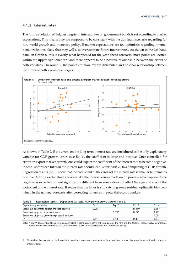
4.1.2. Interest rates

The future evolution of Belgian long-term interest rates on government bonds is set according to market expectations. This means they are supposed to be consistent with the dominant scenario regarding fu-ture world growth and monetary policy. If market expectations are too optimistic regarding interna-tional trade, it is likely that they will also overestimate future interest rates. As shown in the left-hand panel in Graph 8, this is exactly what happened for the year-ahead forecasts: most points are located within the upper-right quadrant and there appears to be a positive relationship between the errors of both variables.17 In round 2, the points are more evenly distributed and no clear relationship between the errors of both variables emerges.

As shown in Table 9, if the errors on the long-term interest rate are introduced as the only explanatory variable for GDP growth errors (see Eq. 2), the coefficient is large and positive. Once controlled for errors on export market growth, one could expect the coefficient of the interest rate to become negative. Indeed, unforeseen hikes in the interest rate should lead, ceteris paribus, to a dampening of GDP growth. Regression results (Eq. 3) show that the coefficient of the errors of the interest rate is smaller but remains positive. Adding explanatory variables like the forecast errors made on oil prices – which appear to be negative as expected but not significantly different from zero – does not affect the sign and size of the coefficient of the interest rate. It seems that the latter is still catching some residual optimistic bias con-tained in the national forecasts after correcting for errors in potential export markets.

Table 9 Regression results – Dependent variable: GDP growth errors (round 1 and 2) Explanatory variables Eq. 1 Eq. 2 Eq. 3 Eq. 4Errors on potential export market growth 0.26** 0.25** 0.25**Errors on long-term interest rate 0.70* 0.27* 0.27*Errors on oil price growth expressed in euros -0.00R2 0.81 0.13 0.83 0.83Note: * and ** denote that the regression coefficient is significantly different from zero at the 10% and the 5% level respectively. Significance

levels were calculated based on standard errors robust to autocorrelation and heteroskedasticity.

17 Note that the points in the lower-left quadrant are also consistent with a positive relation between international trade and

interest rates.

Graph 8 Long-term interest rate and potential export market growth: forecast errors Percentage points


-1.5

-1.0

-0.5

0.0

0.5

1.0

1.5

2.0

-10 -5 0 5 10 15

Long

-ter

m in

tere

st r

ate


Round 1

-1.5

-1.0

-0.5

0.0

0.5

1.0

1.5

-8 -6 -4 -2 0 2 4 6 8

Long

-ter

m in

tere

st r

ate


Round 2

WORKING PAPER 12-17

24

4.2. Impact on CPI growth forecast errors

Even if import prices are endogenous in the MODTRIM model, they are largely determined by interna-tional prices (for which oil prices play a key role) and exchange rate movements.18 As shown in Graph 9, there is a positive correlation between the forecast errors made on the imports deflator and CPI growth. The regression coefficient implies that a one percentage point forecast error on the imports deflator growth generates on average an error of almost 0.2 percentage points on CPI growth forecasts. When correcting the latter for the errors made on the imports deflator growth using this coefficient, the negative bias present in round 2 (see Table 3 in the previous section) is much smaller and the MAE is reduced by 35% in round 1 and by 30% in round 2. Adding the forecast errors made on oil prices ex-pressed in euros does not increase the explanatory power of the previous equation. This result is not surprising though as oil price forecast errors are in principle already included in the global import price errors.

18 The effect of domestic prices on import prices through a pricing to the market strategy by foreign firms is rather limited, see

DE KETELBUTTER et al., op. cit.

Graph 9 Imports deflator and CPI growth: forecast errors (round 1 and 2) Percentage points


y = 0.18xR² = 0.59

-3

-2

-1

0

1

2

3

-10 -8 -6 -4 -2 0 2 4 6 8 10

CPI g

row

th

Imports deflator growth

WORKING PAPER 12-17

25

5. References

BOGAERT, H., DOBBELAERE, L., HERTVELDT, B. and LEBRUN, I. (2006), Fiscal councils, independent forecasts and the budgetary process: lessons from the Belgian case, Working Paper 4-06, Brussels, Federal Planning Bureau.

DE KETELBUTTER, B., DOBBELAERE, L., LEBRUN, I., VANHOREBEEK, F. (2014), A new version of MODTRIM II - An overview of the model for short-term forecasts, Working Paper 05-14, Brussels, Federal Planning Bureau.

DOBBELAERE, L., HERTVELDT, B., HESPEL, E. and LEBRUN, I. (2003), Tout savoir sur la confection du budget économique, Working Paper 17-03, Brussels, Federal Planning Bureau.

DOBBELAERE, L. and HERTVELDT, B. (2004), 10 jaar Economische Begroting: Een terugblik op de kwaliteit van de vooruitzichten, Working Paper 13-04, Brussels, Federal Planning Bureau.

DOBBELAERE, L. and LEBRUN, I. (2012), Track record of the FPB’s short-term forecasts. An update, Work-ing Paper 3-12, Brussels, Federal Planning Bureau.

EUROPEAN COMMISSION (issues from 1995 to 2016), European Economic Forecast, Brussels.

FEDERAL PLANNING BUREAU / NATIONAL ACCOUNTS INSTITUTE (issues from 1994 to 2016), Budget économique – Economische begroting, Brussels.

FEDERAL PLANNING BUREAU (1998), The accuracy of the FPB short-term economic forecasts since 1994, Special Topic, Short Term Update 4-98, pp. 3-4, Brussels.

FEDERAL PLANNING BUREAU (2006), Tools and methods used at the Federal Planning Bureau, Working Paper 7-06, Brussels.

FIORAMANTI, M., GONZÁLEZ CABANILLAS, L., ROELSTRAETE, B. and FERRANDIS VALLTERRA, S. (2016), European Commission’s Forecasts Accuracy Revisited: Statistical Properties and Possible Causes of Forecast Errors, Discussion Paper 27, Brussels, European Commission.

GENBERG, H. and MARTINEZ, A. (2014), On the Accuracy and Efficiency of IMF Forecasts: A Survey and Some Extensions, IEO Background Paper, Washington DC, Independent Evaluation Office of the In-ternational Monetary Fund.

HERTVELDT, B. and LEBRUN, I. (2003), MODTRIM II: A quarterly model for the Belgian economy, Work-ing Paper 6-03, Brussels, Federal Planning Bureau.

LOUNGANI, P. and RODRIGUEZ, J. (2008), Economic Forecasts: Too smooth by far?, World Economics, vol. 9, nr. 2, pp. 1-12.

PAIN, N., LEWIS, C., DANG, T-T., JIN, Y. and RICHERDSON, P. (2014), OECD Forecasts During and After the Financial Crisis – A Post Mortem, Economics Department Working Papers No. 1107, Paris, OECD.

WORKING PAPER 12-17

26

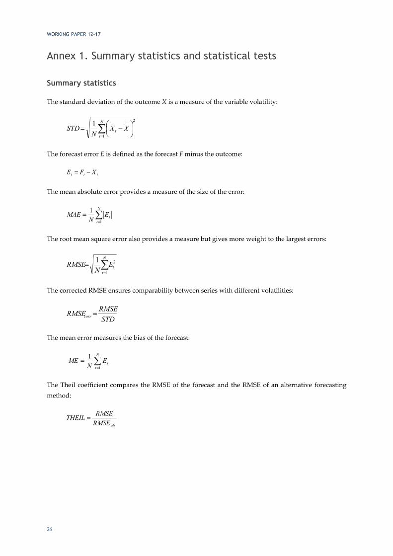
Annex 1. Summary statistics and statistical tests

Summary statistics

The standard deviation of the outcome X is a measure of the variable volatility:

2

1

1∑=

−

⎟⎠⎞

⎜⎝⎛ −=

N

tt XX

NSTD

The forecast error E is defined as the forecast F minus the outcome:

ttt XFE −=

The mean absolute error provides a measure of the size of the error:

∑=

=N

ttEN

MAE1

1

The root mean square error also provides a measure but gives more weight to the largest errors:

∑=

=N

ttEN

RMSE1

21

The corrected RMSE ensures comparability between series with different volatilities:

STDRMSERMSEcorr =

The mean error measures the bias of the forecast:

∑=

=N

ttEN

ME1

1

The Theil coefficient compares the RMSE of the forecast and the RMSE of an alternative forecasting method:

altRMSERMSETHEIL =

WORKING PAPER 12-17

27

Statistical tests

Bias

Testing for the statistical significance of the bias is done by regressing the forecast error on a constant:

ttE εα +=

The absence of bias requires α = 0. The restriction is tested with the t-statistic that is always corrected for the (possible) presence of autocorrelation and/or heteroskedasticity in the residu-als.

Persistence of forecast errors

The persistence of forecast errors is tested by checking the residuals from the above-mentioned equation for serial correlation. This test is carried out based on Ljung-Box Q-statistics that are asymptotically distributed as a χ² with the degrees of freedom equal to the number of autocorrelations that is tested. Note that the test for second order serial correlation tests the joint significance of first and second order serial correlation.

Revisions

Testing for the absence of bias in the revisions is done by regressing the revisions on a constant:

ttF εα +=Δ

The absence of bias requires α = 0. The restriction is tested with the t-statistic.

Testing for independent revisions is done by regressing revisions in round 3 on revisions in round 2:

ttt FF εβα 23 Δ+=Δ

Independent revisions require β = 0. The restriction is tested with the t-statistic.

Economic analyses and forecasts...task to deliver the macroeconomic forecasts that are used to set...

Documents

Transcript of Economic analyses and forecasts...task to deliver the macroeconomic forecasts that are used to set...