![[Spanos] Statistical Foundations of Econometric Modelling](https://static.fdocuments.net/doc/165x107/55cf8583550346484b8eda22/spanos-statistical-foundations-of-econometric-modelling.jpg)
Econometric Modelling Based on Pattern Recognition via the … · 2020-01-08 · Econometric...
50
1 Department of Economics University of Victoria Working Paper EWP0101 ISSN 1485-6441 Econometric Modelling Based on Pattern Recognition via the Fuzzy c-Means Clustering Algorithm David E. A. Giles Department of Economics University of Victoria & Robert Draeseke B.C. Ministry of Aboriginal Affairs January, 2001 Abstract In this paper we consider the use of fuzzy modelling in the context of econometric analysis of both time-series and cross-section data. We discuss and demonstrate a semi-parametric methodology for model identification and estimation that is based on the Fuzzy c-Means algorithm that is widely used in the context of pattern recognition, and the Takagi-Sugeno approach to modelling fuzzy systems. This methodology is exceptionally flexible and provides a computationally tractable method of dealing with non-linear models in high dimensions. In this respect it has distinct theoretical advantages over non-parametric kernel regression, and we find that these advantages also hold empirically in terms of goodness-of-fit in a selection of economic applications. Acknowledgement: We are grateful to George Judge, Joris Pinkse, Ken White, and participants in the University of Victoria Econometrics Colloquium for their helpful comments. Keywords: Fuzzy logic, fuzzy sets, fuzzy c-means algorithm, pattern recognition, semi-parametric modelling, curse of dimensionality JEL Classifications: C14, C49, C51 Author Contact: Professor David Giles, Department of Economics, University of Victoria, P.O. Box 1700 STN CSC, Victoria, B.C., Canada V8W 2Y2 Email: [email protected]; FAX: (250) 721-6214; Voice: (250) 721-8540
Transcript of Econometric Modelling Based on Pattern Recognition via the … · 2020-01-08 · Econometric...

1
Department of Economics University of VictoriaWorking Paper EWP0101 ISSN 1485-6441
Econometric Modelling Based on Pattern Recognition via theFuzzy c-Means Clustering Algorithm
David E. A. Giles
Department of EconomicsUniversity of Victoria
&
Robert Draeseke
B.C. Ministry of Aboriginal Affairs
January, 2001
Abstract
In this paper we consider the use of fuzzy modelling in the context of econometric analysis ofboth time-series and cross-section data. We discuss and demonstrate a semi-parametricmethodology for model identification and estimation that is based on the Fuzzy c-Meansalgorithm that is widely used in the context of pattern recognition, and the Takagi-Sugenoapproach to modelling fuzzy systems. This methodology is exceptionally flexible and provides acomputationally tractable method of dealing with non-linear models in high dimensions. In thisrespect it has distinct theoretical advantages over non-parametric kernel regression, and we findthat these advantages also hold empirically in terms of goodness-of-fit in a selection of economicapplications.
Acknowledgement: We are grateful to George Judge, Joris Pinkse, Ken White, and participants in the University of Victoria Econometrics Colloquium for their helpful comments.
Keywords: Fuzzy logic, fuzzy sets, fuzzy c-means algorithm, pattern recognition, semi-parametric modelling, curse of dimensionality
JEL Classifications: C14, C49, C51
Author Contact: Professor David Giles, Department of Economics, University of Victoria,P.O. Box 1700 STN CSC, Victoria, B.C., Canada V8W 2Y2Email: [email protected]; FAX: (250) 721-6214; Voice: (250) 721-8540

2
1. Introduction
The specification and estimation of any econometric relationship poses significant challenges.
This is especially true when it comes to the choice of functional form, as the latter is not always
suggested or prescribed by the underlying economic theory. Any mis-specification of the
functional form of an econometric model can have serious consequences for statistical inference -
for example, the parameter estimates may be inconsistent. In response to the rigidities associated
with explicit and rigid parametric functional relationships, and to avoid the consequences of their
mis-specification, a more flexible non-parametric approach to their formulation and estimation is
often very attractive (e.g., Pagan and Ullah, 1999).
Such non-parametric estimation does, however, have its drawbacks. Most notably, in order to
perform well, multivariate kernel regression requires a reasonably large sample of data, and it
founders when the number of explanatory variables grows. With regard to the latter point there
are really two problems. First, there is evidence that the small-sample properties of the
multivariate kernel estimator can be quite unsatisfactory (e.g., Silverman, 1986). Second, the rate
of convergence of the kernel estimator decreases as the dimension of the model grows - this is the
so-called “curse of dimensionality”. Recently, Coppejans (2000) has dealt with this problem by
using cubic B-spline estimation in conjunction with earlier results from Kolmogorov (1957) and
Lorentz (1966) that enable a function of several variables to be represented as superpositions of
functions of a single variable.
There is considerable appeal in the prospect of finding an approach to the formulation and
estimation of econometric relationships that are highly flexible in terms of their functional form;
make minimal parametric assumptions; perform well with either small or large data-sets; and are
computationally feasible even in the face of a large number of explanatory variables. In this
paper we use some of the tools of fuzzy set theory and fuzzy logic in the pursuit of just such an
objective.
These tools have been applied widely in many disciplines since the seminal contributions of
Zadeh (1965, 1987) and his colleagues. These applications are numerous in such areas as
computer science, systems analysis, and electrical and electronic engineering. The construction
and application of “expert systems” is widespread in domestic appliances, motor vehicles, and
commercial machinery. The use of fuzzy sets and fuzzy logic in the social sciences appears to

3
have been limited mainly to psychology, with very little application to the analysis of economic
problems and economic data. There are a few such examples in the field of social choice - for
example, Dasgupta and Deb (1996), Richardson (1998), and Sengupta (1999). In the area of
econometrics, however, there have been surprisingly few applications of fuzzy set/logic
techniques. Indeed, we are aware of only four such examples.
Josef et al. (1992) used this broad approach in the context of modelling with panel data.
LindstrCm (1998) used fuzzy logic in a rather different way to model fixed investment in Sweden
on the basis of the level and variability in the real interest rate. More specifically, he generated an
index for aggregate investment using fuzzy sets and operators to combine the imprecise
information associated with the interest rate. He found that this approach provided a simple
method of modelling inherent non-linearities in a flexible (non-parametric) manner. It should be
noted that LindstrCm's analysis involved no statistical inference, as such. This same technique
was used by Draeseke and Giles (1999, 2000) to generate an index of the New Zealand
underground economy, and it has now been programmed into the SHAZAM (2000) econometrics
package. The advantage of using this particular technique in that context was that the variable of
interest is intrinsically unobservable.
Shepherd and Shi (1998) used fuzzy set/logic theory in a rather different manner in their analysis
of U.S. wages and prices. Their modelling technique involved clustering the data into fuzzy sets,
estimating the relationship of interest over each set, and then combining each sub-model into a
single overall model by using the membership functions associated with the clustered data
together with the Takagi and Sugeno (1985) approach to fuzzy systems. Their analysis also
highlighted the ability of such fuzzy analysis to detect and measure non-linear relationships in a
very flexible way, even though the underlying sub-models may be linear. Indeed, this is a specific
and attractive feature of the Takagi-Sugeno analysis. In this paper we draw on the approach of
Shepherd and Shi and adapt it to model a number of interesting relationships. We discuss some of
the issues that arise when adopting this semi-parametric approach in the specification and
estimation of an econometric model, and by way of specific practical applications we illustrate
some of its merits relative to standard parametric regression and conventional (kernel) non-
parametric regression.
The use of fuzzy sets and fuzzy logic is just one of several possible approaches within the general
area of expert systems and artificial intelligence. In the context that is of interest to us here, an

4
obvious competitive approach is that based on (artificial) neural networks (e.g., Bishop, 1995;
White, 1992; White and Gallant, 1992). Neural networks also facilitate the modelling of nonlinear
relationships whose underlying form is not parametrically constrained at the outset. However, our
adaptation of the Takagi-Sugeno/Shepherd-Shi (TSSS) methodology has an important and
appealing advantage over the use of neural networks. Namely, the basic relationships that are
estimated have a direct economic interpretation, and they can be related to the underlying
economic theory in a useful way. The same is not generally true in the case of neural networks.
Moreover, and as we shall see in more detail below, the TSSS methodology is computationally
efficient, especially in as much as it requires only one “pass” through the data. In contrast, neural
networks usually have to be “trained”, and this involves more protracted computations.
In the next section we outline the background concepts in fuzzy set/logic theory that we will be
using. A crucial component of our analysis is the implementation of the so-called “fuzzy c-
means” algorithm to partition the data-set in a flexible manner, and this algorithm is considered in
some detail in section 3. In section 4 we describe our variant of the TSSS modelling procedure,
and section 5 presents the results associated with several illustrative empirical applications of this
fuzzy technology. Some concluding remarks are given in section 6.
2. Fuzzy Sets and Fuzzy Logic
As was noted above, fuzzy logic relates to the notion of fuzzy sets, the theoretical basis for which
is usually attributed to Zadeh (1965). Under regular set theory, elements either belong to some
particular set or they do not. Another way of expressing this is to say that the “degree of
membership” of a particular element with respect to a particular set is either unity or zero. The
boundaries of the sets are hard, or “crisp”. In contrast to this, in the case of fuzzy sets, the degree
of membership may be any value on the continuum between zero and unity, and a particular
element may be associated with more than one set. Generally this association involves different
degrees of membership with each of the fuzzy sets. Just as this makes the boundaries of the sets
fuzzy, it makes the location of the centroid of the set fuzzy as well.
To consider an illustrative situation relating to a single economic variable, suppose we wish
distinguish between situations of excess supply and those of excess demand in relation to the
price of some good. In traditional set theory we would have a situation such as:

5
Ss = {p: p > p*}
Sd = {p: p < p*}
Se = {p*}
as the crisp sets representing those prices associated with excess supply, excess demand, and the
equilibrium price (p*}, respectively. Any particular price, say $5, would definitely be in one and
only one of these sets. That is, if its degree of membership with Si is denoted ui, then uj = 1
implies that uk = 0, for all k � j; for k, j = s, d, e. In contrast to this, in a fuzzy set framework the
sets Ss, Sd and Se would not have sharp boundaries and a particular price (such as $5) would be
associated to some degree or other with each of these sets. For instance, its degrees of
membership might be us = 0.2, ud = 0.3, ue = 0.5. Note that although the ui's sum to unity in this
example, in general they need not, and they should not be equated with the “probabilities” that the
price of $5 lies in each set.
It should also be noted that in the example above, the concepts involved are defined in a crisp
manner: “excess supply”, “excess demand”, and “equilibrium”. More generally, fuzzy set theory
is just as capable of handling vague linguistic concepts, such as “a rather high price”, or “a very
low demand”. So, we could broaden the above example to allow for fuzzy sets involving prices
associated with “a very high excess supply”, “a moderate excess supply”, “a small excess
supply”, and so on. Again, the boundaries of these sets would be fuzzy, and degrees of
membership would map prices to the sets.
The application of the inductive premise to fuzzy concepts poses some difficulties – not all of the
usual laws of set theory are satisfied. In particular, the “law of the excluded middle” is violated,
so a different group of set operators must be adopted. So, for example, the “union” operator is
replaced by the “max” operator, “intersection” is replaced by “min”, and “complement” is
replaced by subtraction from unity. Under these “fuzzy” operators the commutative, associative,
distributive, idempotency, absorption, excluded middle, involution, and De Morgan’s laws are all
satisfied in the context of fuzzy sets. For example if the universal set is U={a, b, c, d} let the
fuzzy sets S1 and S2 be defined as S1 = {0.4/a, 0.5/b, 1/d} and S2 = {0.1/a, 0.2/b, 0.5/c, 0.9/d}.
Here, the numbers are the “degrees of membership” which map the elements of U to S1 and S2.
Then, A∪ B = {0.4/a, 0.5/b, 0.5/c, 1/d} and A∩B = {0.1/a, 0.2/b, 0/c, 0.9/d}, S1c = {0.6/a, 0.5/b,
1/c, 0/d}, and S2c = {0.9/a, 0.8/b, 0.5/c, 0.1/d}.

6
Fuzzy sets can be used in conjunction with logical operators in a manner that will enable us to
construct models in a flexible way. More specifically, we can use the degrees of membership that
associate the values of one or more input variables with different fuzzy sets, together with logical
“IF”, “THEN”, “AND” operations, to derive membership values that associate an output variable
with one or more fuzzy sets. For example, in the case of the demand for a particular good, we
might have a fuzzy rule of the form:
“IF the own-price of the good is quite low, AND the price of the only close
substitute good is rather high, THEN the demand for the good in question will be
fairly high.”
Or, to anticipate one of our empirical examples later in this paper:
“IF the interest rate is fairly high, AND income (output) is relatively low, THEN
the demand for money will be quite low.”
Of course, in general, there will be more than one fuzzy rule, and the output variable may have
potential membership in more than one fuzzy set:
Rule 1: “IF the interest rate is fairly high, AND income (output) is relatively low, THEN
the demand for money will be quite low.”
Rule 2: “IF the interest rate is average, AND income (output) is relatively high, THEN
the demand for money will be moderately high.”
In such situations, a fuzzy outcome for the output variable could be inferred by taking account of
the relevant membership values, and the MAX/MIN operators associated with fuzzy sets.
However, a fuzzy outcome is not usually adequate. For instance, in the last example, there is only
limited interest in knowing that the fuzzy model predicts that in a certain period the demand for
money will be “moderately high”, or “quite low”. It would be much more helpful to know (for
example) that the model predicted a demand of $10million. In other words, we need a way of
“de-fuzzifying” the predictions of the model.
The Takagi and Sugeno (1985) and Sugeno and Kang (1985) approach to dealing with this issue
involves modfiying the above methodology to one that involves rules of the form:

7
Rule 1': “IF the interest rate (r) is fairly high, AND income (Y) is relatively low, THEN
the demand for money is M = f1 (r, Y) = M1.”
Rule 2': “IF the interest rate (r) is average, AND income (Y) is relatively high, THEN
the demand for money is M = f2 (r, Y) = M2.”
Here, f1 and f2 are crisp, and generally parametric, functions which yield numerical values for M.
In their simplest form these functions would be linear relationships. The various values (M1, M2,
etc.) emerging from these rules can then be combined by taking a weighted average, based on the
degrees of membership associated with the input variables and the fuzzy input sets. This is
described in more detail in section 4 below. First, however, we need to give further consideration
to the definition and construction of the fuzzy input sets, and this involves grouping or
“clustering” the input data appropriately.
3. The Fuzzy c-Means Algorithm
3.1 Overview of the Algorithm
In our modelling analysis, which is described in detail in the next section, we need to determine
the partitioning of the sample data for each explanatory (input) variable into a number of clusters.
These clusters have “fuzzy” boundaries, in the sense that each data value belongs to each cluster
to some degree or other. Membership is not certain, or “crisp”. Having decided upon the number
of such clusters to be used, some procedure is then needed to locate their mid-points (or more
generally, their centroids) and to determine the associated membership functions and degrees of
membership for the data-points. To this end, Shepherd and Shi (1998) used a variant of the “fuzzy
c-means” (FCM) algorithm. (The latter is sometimes termed the fuzzy k-means algorithm in the
literature.) The FCM algorithm is really a generalization of the “hard” c-means algorithm. It
appears to date from Ruspini (1970), although some of the underlying concepts were explored by
MacQueen (1967). The FCM algorithm is closely associated with such early contributors as
Bezdek (1973) and Dunn (1974, 1977), and is widely used in such fields as pattern recognition,
for instance.
The algorithm provides a method of dividing up the “n” data-points into “c” fuzzy clusters (where
c < n), while simultaneously determining the locations of these clusters in the appropriate space.
The data may be multi-dimensional, and the metric that forms the basis for the usual FCM is
“squared error distance”. The underlying mathematical basis for this procedure is as follows. Let

8
xk be the k’th (possibly vector) vector data-point (k = 1, 2, ...., n). Let vi be the center of the i’th.
(fuzzy) cluster (i = 1, 2, ....., c). Let dik = || xk - vi || be the distance between xk and vi , and let uik be
the “degree of membership” of data-point “k” in cluster “i”, where :
The objective is partition the data-points into the “c” clusters, and simultaneously locate those
clusters and determine the associated “degrees of membership”, so as to minimize the functional
There is no prescribed manner for choosing the exponent parameter, “m”, which must satisfy 1 <
m < �. In practice, m = 2 is a common choice. In the case of crisp (hard) memberships, m = 1.
In broad terms, the FCM algorithm involves the following steps:
1. Select the initial location for the cluster centres.
2. Generate a (new) partition of the data by assigning each data-point to its closest cluster
centre.
3. Calculate new cluster centres as the centroids of the clusters.
4. If the cluster partition is stable then stop. Otherwise go to step 2 above.
In the case of fuzzy memberships, the Lagrange multiplier technique generates the following
expression for the membership values to be used at step 2 above:
Notice that a singularity will arise if djk = 0 in the above expression. This occurs if, at any point a
cluster centre exactly coincides with a data-point. This can be avoided at the start of the algorithm
and generally will not arise subsequently in practice due to machine precision. If the
memberships of data-points to clusters are “crisp” then
uik = 0 ; � i � j,
ujk = 1 ; j s.t. djk = min.{dik, i = 1, 2, ...., c}.
J U v u dk
n
ik
i
cm
ik( , ) ( ) ( ) .===
∑∑11
2
u d dik ik
j
n
jkm=
=
−∑1 2
1
2 1 1/ [( ) / ( ) ]{ } ./ ( )
( ) .u ik
i
c
==∑ 1
1

9
The updating of the cluster centres at step 3 above is obtained via the expression
The fixed-point nature of this problem ensures the existence of a solution. See Bezdek (1981,
Chapter 3) for complete and more formal mathematical details. As will be apparent, the FCM
algorithm is simple to program. We have chosen to do this using standard commands in the
SHAZAM (2000) econometrics package - this makes it convenient to compare our results with
those from the other standard regression modelling techniques that are available in that package.
3.2 Some Computational Issues
Among the issues that arise in the application of the FCM are the following. First, a value for the
number of clusters and the initial values for their centres have to be provided to start the
algorithm. It appears that the results produced by the FCM algorithm can be sensitive to the
choice of these start-up conditions. Second, being based on a “squared error” measure of distance,
the algorithm can be sensitive to noise or outliers in the data.
In relation to the first of these issues, several proposals have been made. Among these are the
following. Linde et al. (1980) proposed the Binary Splitting (BS) technique to initialize the
clusters. The disadvantage of the BS technique is that it requires at least 10 or 20 data points in
each cluster, and in practice this may not be attainable. Huang and Harris (1993) extended this
approach to the “Direct Search Binary Splitting” technique. Tou and Gonzales (1974) proposed
the “Simple Cluster-Seeking” (SCS) method, which deals not only with the initial value issue, but
also provides the clusters themselves. However, the SCS technique is not invariant to the order in
which the data points are considered, and it also depends on certain “threshold” settings.
Yager and Filev (1992) introduced the so-called “Mountain Method” for deciding on the initial
values. Their approach is apparently simple, but it becomes computationally burdensome in the
context of multi-dimensional data. Consequently, Chiu (1994) proposed a modification of their
approach, called “Subtractive Clustering”, that does not suffer the same problem. This is the
v u x u i ci ikm
k
n
k ikm
k
n
= == =
∑ ∑[ ( ) ] / [ ( ) ] ; , , . . . . , .1 1
1 2

10
approach used by Shepherd and Shi (1998). Babu and Murty (1993) used genetic algorithms to
initialize the clusters, and Katsavounidis et al. (1994) proposed a further method (KKZ). More
recently, Al-Daoud and Roberts (1996) proposed two initialization methods that appear to be
especially useful in the context of very large data sets, and which out-performed both the KKZ
and SCS techniques with their test data.
In relation to the second of the above issues (noise and outliers in the data), there have again been
a number of contributions. Among these are the following. Following on from earlier
(computationally expensive) contributions by Weiss (1988) and Jolion and Rosenfeld (1989),
Davé (1991) modified the FCM algorithm (still retaining a “squared error” distance concept) so
that noisy data points are effectively allocated to a “noise cluster”, rather than being allocated to
other clusters, and so “contaminating” the latter. More recently, Keller (2000) suggested another
related modification involving the use of a modified objective function with a weighting factor
added for each data point - the objective being to assign a kind of influence factor to the single
data points. Some authors have taken up the usual techniques used in the statistical literature to
deal with the sensitivity of least squares to the problem of outliers. That is to say, methods of
“robust estimation” have been incorporated into the FCM algorithm, and these have included “M-
estimation”, “trimmed least squares”, and “least absolute deviations” alternatives to the least
squares component of the FCM algorithm. A recent example of this approach is that of Frigui and
Krishnapuram (1996), who integrate M-estimation into the FCM algorithm. They provide a
computationally attractive generalization of the FCM algorithm that deals with both the
identification of the number of clusters and the allocation of data points to these clusters
simultaneously, and which is robust to noise and outliers.
4. Fuzzy Econometric Modelling
In this section we describe the TSSS methodology that we subsequently apply to a number of
econometric model estimation problems. The discussion here is quite expository, and we begin by
outlining the analysis in the very simple case where there is a single input variable (other than,
perhaps, a constant intercept). So, the fuzzy relationship is of the form:
y f x= +( ) ε
11
where the functional relationship will typically involve unknown parameters, and � is a random
disturbance term. While there is no need to make any distributional assumptions about the latter,
if this is done then these can be taken into account in the subsequent analysis. If the disturbance
has a zero mean, the fuzzy function represents the conditional mean of the output variable, y. To
this extent, the framework is the same as that which is adopted in non-parametric kernel
regression.
The identification and estimation of the fuzzy model then proceeds according to the following
steps:
Step 1: Partition the sample observations for x into c fuzzy clusters, using the FCM
algorithm. This generates the membership values for each x-value with respect to
each cluster, and implicitly it also defines a corresponding partition of the data
for y.
Step 2: Using the data for each fuzzy cluster separately, fit the models:
In particular, if the chosen estimation procedure is least squares, then
Step 3: Model and predict the conditional mean of y using:
where uik is the degree of membership of the k’th. value of x in the i’th. fuzzy
cluster, and bim is the least squares estimator of �im (m = 0, 1) obtained using the
i’th. fuzzy partition of the sample.
Step 4: Calculate the predicted “input-output relationship” (i.e., the derivative) between x
and the conditional mean of y:
y f x j n i cij i ij ij i= + = =( ) ; , . . . . , ; , . . . . ,ε 1 1
y x j n i cij i i ij ij i= + + = =β β ε0 1 1 1; , . . . . , ; , . . . . ,
[ ]� ( ) / ; , . . . . ,y b b x u u k nki
c
i i k iki
c
ik= +
=
= =∑ ∑
10 1
1
1
[ ]( � / ) ( ) / ; , ,∂ ∂y x b u u k nk ki
c
i iki
c
ik=
=
= =∑ ∑
11
1
1 ��

12
So, the fuzzy predictor of the conditional mean of y is a weighted average of the linear predictors
based on the fuzzy partitioning of the explanatory data, with the weights (membership values)
varying continuously through the sample. This latter feature enables non-linearities to be
modelled effectively. In addition, it can be seen that the separate modelling over each fuzzy
cluster involves the use of fuzzy logic of the form “IF the input data are likely to lie in this
region, THEN this is likely to be the predictor of the output variable”, etc.. The derivative of the
conditional mean with respect to the input variable also has this weighted average structure, and
the same potential for non-linearity.
Note that this modelling strategy is essentially a semi-parametric one. The parametric
assumptions could be relaxed further by using kernel estimation to fit each of the cluster sub-
models at Step 2 above, in which case the estimated derivatives (rather than coefficients) would
be weighted at Steps 3 and 4, instead of the parameter estimates. However, some limited
experimentation with this variation of the modelling methodology, in the context of the empirical
applications described in the next section, yielded results that were inferior to those based on least
squares.
Of course, in general we will be concerned with models that have more than one input
(explanatory) variable:
In such cases the steps in the above fuzzy modelling procedure are extended as follows, assuming
a linear least squares basis for the analysis for expository purposes:
Step 1': Separately partition the n sample observations for each xr into cr fuzzy clusters
(where r = 1, 2, ....,p), using the FCM algorithm. This generates the membership
values for each observation on each x variable with respect to each cluster.
Step 2': Consider all c possible combinations of the fuzzy clusters associated with the p
input variables, where
y f x x x p= +( , , . . . . . . . , )1 2 ε
c crr
p
==
∏1
13
and discard any for which the intersections involve negative degrees of freedom
(nr < p). Let the number of remaining cluster combinations be c'.
Step 3': Using the data for each of these c' fuzzy clusters separately, fit the models:
Step 4': Model and predict the conditional mean of y by using:
where
Here, �ij is a “selector” that chooses the membership value for the j’th. fuzzy
cluster (for the r’th. input variable) if that cluster is associated with the i’th.
cluster combination (i = 1, 2, …., c'); and bim is the least squares estimator of
�im obtained using the i’th. fuzzy partition of the sample.
Step 5': Calculate the predicted “input-output relationships” (i.e., the derivatives)
between the conditional mean of y and each input variable, xr:
Comparing these steps with those in the case of a single input variable, it is clear that the
computational burden associated with the fuzzy modelling increases at the same rate as in the
case of multiple linear regression as additional explanatory variables are added to the model.
Under very mild conditions on the input data and the random error term, fitting the sub-models
over each fuzzy cluster yields a weakly consistent predictor of the conditional mean of the output
variable. The partitioning of the sample into fuzzy clusters, and the determination of the
associated membership functions, involves using only the explanatory variable data in a non-
stochastic manner. If the explanatory variables are exogenous then so will be the membership
y x x x j n i cij i i ij i ij ip p ij ij i= + + + + + = =β β β β ε0 1 1 2 2 1 1�� ; , . . . . , ; , . . . . , '
[ ]( � / ) ( ) / ; , ; , ,' '
∂ ∂y x b w w r p k nk rki
c
ir r iki
c
ik=
= =
= =∑ ∑
1 1
1 1�� ��
[ ]� ( ) / ; , . . . . ,'
y b b x b x w w k nki
c
i i k ip pk iki
c
ik= + + +
=
= =∑ ∑
10 1 1
1
1��
w u i ci kr
p
ij r jk= ==
∏1
1δ ; , , '��

14
values that are used to construct the weighted averages of the least squares predictors in Step 4
above. Then, the fuzzy predictor of the conditional mean of y at Step 4 will be weakly consistent.
5. Some Applications
We have applied the fuzzy econometric modelling described above to a number of illustrative
estimation and smoothing problems, and the associated results are described in this section. As
was noted in the context of the FCM algorithm above, the computation for these applications was
undertaken by writing command code for the SHAZAM (2000) econometrics package. We have
chosen a number of simple examples that involve both cross-section and time-series data, and
which involve various degrees of model complexity in terms of the number of explanatory
variables involved.
5.1 Modelling the Earnings-Age Profile
In our first application the relationship of interest is one that explains the logarithm of earnings as
a function of age, the latter being a proxy for years of work experience. Typically, in the labour
economics literature, this relationship has been modelled by using standard parametric regression,
typically with both age and its square being included as regressors. This quadratic relationship
allows for the fact that earnings would be expected to increase with age through much of the
working life, but that the rate of increase declines with age (e.g., Heckman and Polachek, 1974;
Mincer, 1974). Mincer relates the concave quadratic function to the behaviour that is implied by
the optimal distribution of human capital investment over an agent's life-cycle, but more recently
Murphy and Welsch (1990) have provided evidence that a quartic relationship performs more
satisfactorily than a quadratic one.
Our own application involves a cross-section data-set relating to the earnings and ages of a
sample 205 Canadian individuals, all of whom had the same number of years of schooling. These
data come from the 1971 Canadian Census Public Use Tapes, and have been used in various
parametric and non-parametric studies by Ullah (1985), Singh et al. (1987), Pagan and Ullah
(1999, 152-157) and van Akkeren (2001). As Pagan and Ullah discuss, simple polynomial models
result in a smooth concave relationship, but when a non-parametric kernel estimator is used the
fitted relationship exhibits a “dip” around the age of forty to forty five. Interestingly, the same
effect is obtained by van Akkeren (2001, Table 3.5) via their data based information theoretic

15
(DBIT) estimation procedure. A possible explanation for this dip is offered by Pagan and Ullah
(1999, 154):
....(it may be due to) “the generation effect, because the cross section data represent the
earnings of people at a point in time who essentially belong to different generations. Thus
the plot of earnings represents the overlap of the earnings trajectories of different
generations. Only if the sociopolitical environment of the economy has remained stable
intergenerationally can we assume these trajectories to be the same. But this is not the
case; one obvious counterexample being the Second World War. Therefore, the dip in the
nonparametric regression might be attributed to the generation between 1935 and 1945.”
Figure 1 illustrates this effect with the Canadian earnings data. There, we show the results of
fitting a quadratic relationship by the method of least squares, as well as a non-parametric kernel
estimate. The latter uses a Normal kernel with the approximately optimal bandwidth described by
Silverman (1986, 45). Also shown in that figure is the result of applying our fuzzy regression
analysis with three fuzzy clusters and m = 2. (The results were not sensitive to the latter choice of
value for the exponent parameter in the application of the FCM algorithm.) Some of the details
associated with the clustering of the data and the estimation of sub-models appear in Table 1,
together with a comparison of the quality of the overall “fit” of the fuzzy model as compared with
the non-parametric kernel and quadratic least squares models. In part (a) of that table we see that
the sub-model estimates (based on each of the three fuzzy clusters) are fundamentally different
from each other. When these are combined on the basis of the associated membership functions
(which are depicted in Figure 2) we are able to fit a flexible non-linear relationship. In part (b) of
Table 1 we see that the fuzzy model fits the data better than the non-parametric model and
virtually as well as the quadratic least squares model, on the basis of percent root mean squared
error. This quadratic penalty function actually favours least squares, and the fuzzy model emerges
as the clear winner when the comparison is based on percent mean absolute error.
The sensitivity of the fuzzy econometric modelling results to the chosen number of fuzzy clusters
is illustrated in Figure 3, where the results for c = 3 and c = 4 are compared (with m = 2). The
latter results appear to “over-fit” the data to some degree, and our preference is for the results
shown in Figure 1. The general shape of the fit of the fuzzy regressions reinforces the principal
result of the non-parametric estimation (and the DBIT results of van Akkernen (2001)). We see
an even more pronounced “dip” than in the case of the non-parametric results, with the minimum

16
occurring at an age of forty one (rather than forty four), and the adjacent peaks occurring at ages
of thirty three and forty eight (rather than thirty eight and fifty one).
Figure 2: Membership Functions for Fuzzy Regression (c=3; m=2)
0
0.1
0.2
0.3
0.4
0.5
0.6
0.7
0.8
0.9
1
21 23 25 27 29 31 33 35 37 39 41 43 45 47 49 51 53 55 57 59 61 63 65
Age
Deg
ree
of
Mem
ber
ship
u1
u2
u3
Figure 1: Alternative Estimates of the Earnings-Age Profile
11.0
11.5
12.0
12.5
13.0
13.5
14.0
14.5
15.0
20 25 30 35 40 45 50 55 60 65
Age
Lo
gar
ith
m o
f E
arn
ing
s
Actual
OLS
Non-Parametric
Fuzzy (3)

17
Table 1: Fuzzy Regression Results for Earnings-Age Data
(c = 3; m = 2)
(a) Sub-Model Results
Fuzzy Ranked Cluster Slope Intercept
Cluster Observations Centre (t-value) (t-value)
1 1 to 77 25.7421 0.1194 10.1199
(21 to 32 years) (6.74) (21.68)
2 78 to 148 39.7241 -0.0180 14.3870
(33 to 47 years) (-1.31) (26.22)
3 149 to 205 55.1273 -0.0475 16.2073
(48 to 65 years) (-2.53) (15.69)
(b) Comparative Model Performances*
Least Squares Non-Parametric Fuzzy
%RMSE 4.403 4.459 4.406
%MAE 3.017 3.014 2.992
* %RMSE = Percent root mean squared error of fit.
%MAE = Percent mean absolute error of fit.

18
5.2 An Aggregate Consumption Function
Our second example involves the estimation of a naive aggregate consumption function for the
U.S.A., using monthly seasonally adjusted time-series data for personal consumption
expenditures and real disposable personal income. The data are published by the Bureau of
Economic Analysis at the U.S. Department of Commerce (2000), and are in real 1996 billions of
dollars. The sample period is January 1967 to June 2000 inclusive. The model explains
consumption expenditure simply as a function of disposable income. No dynamic effects or other
explanatory variables are taken into account.
In this case we found that basing the analysis on four fuzzy clusters produced marginally better
results than those based on three clusters. Figure 4 compares the “fit” of the fuzzy model with
obtained by simple least squares, and the corresponding comparison is made with a non-
parametric kernel fit in Figure 5. The latter was obtained with the same kernel and window
choices as in the previous example, and m = 2 was used again as the exponent parameter in the
application of the FCM algorithm. As can be seen in these two figures, the fuzzy model “tracks”
Figure 3: Sensitivity of Fuzzy Modelling to Number of Clusters
12.5
12.7
12.9
13.1
13.3
13.5
13.7
13.9
21 23 25 27 29 31 33 35 37 39 41 43 45 47 49 51 53 55 57 59 61 63 65
Age
Lo
gar
ith
m o
f In
com
e
Non-Parametric
Fuzzy (4)
Fuzzy (3)

19
the data much more satisfactorily than do either of its competitors, and this is borne out by the
percent root mean square errors and percent mean absolute errors that are reported in Table 2.
The close similarity between the results based on three and four fuzzy clusters is clear in Figure 6,
and the %RMSE and %MAE values when c = 3 are 1.327 and 1.033 respectively. The
membership functions for the Fuzzy (4) model appear in Figure 7.
The economic interpretation of the various fitted models is also interesting. In the linear least
squares model the slope parameter is the (constant) marginal propensity to consume (m.p.c.), and
is estimated to be 0.9598 (t = 270.39) from our sample. In the case of the non-parametric model
the estimated derivatives (which represent the changing m.p.c.) range in value from 0.3134 to
1.2427 as the level of disposable income varies. This is shown in Figure 8, where the income data
have been ranked into ascending order. Values of the m.p.c. in excess of unity make no sense in
economic terms, and the extreme and unusual pattern of the plot of the non-parametrically
estimated m.p.c.’s in Figure 8 suggests that these results should be treated with extreme
skepticism. Also given in that figure are the corresponding results for the Fuzzy (4) and Fuzzy (3)
models. In both of these cases the plots are much more reasonable than that for the non-
parametric model, with the estimated m.p.c.’s for the Fuzzy (3) model lying in a somewhat
narrower band than those for the preferred Fuzzy (4) model. The latter m.p.c.’s range from 0.8061
to 1.1705 in value. The few estimates in excess of unity are still troublesome, of course, but apart
from these, the derived m.p.c. values are more plausible economically than are those resulting
from the non-parametric kernel estimation, or from the (highly restrictive) least squares model.

20
Figure 5: U.S. Consumption Model (Monthly 1967M1 - 2000M6)
1800
2300
2800
3300
3800
4300
4800
5300
5800
1 14 27 40 53 66 79 92 105
118
131
144
157
170
183
196
209
222
235
248
261
274
287
300
313
326
339
352
365
378
391
Observation Number
Bill
ion
s o
f 19
96 D
olla
rs
Actual
Non-Parametric
Fuzzy (4)
Figure 4: U.S. Consumption Model (Monthly 1967M1 - 2000M6)
1800
2300
2800
3300
3800
4300
4800
5300
5800
1 14 27 40 53 66 79 92 105
118
131
144
157
170
183
196
209
222
235
248
261
274
287
300
313
326
339
352
365
378
391
Observation Number
Bill
ion
s o
f 19
96 D
olla
rs
Actual
OLS
Fuzzy (4)

21
Figure 6: Sensitivity of Fuzzy Consumption Model to Number of Fuzzy Clusters
1800
2300
2800
3300
3800
4300
4800
5300
5800
1 14 27 40 53 66 79 92 105
118
131
144
157
170
183
196
209
222
235
248
261
274
287
300
313
326
339
352
365
378
391
Observation Number
Bill
ion
s o
f 19
96 D
olla
rs
Fuzzy (3)
Fuzzy (4)
Figure 7: Membership Functions for Fuzzy Regression(c=4; m=2)
0.0
0.1
0.2
0.3
0.4
0.5
0.6
0.7
0.8
0.9
1.0
2000 2500 3000 3500 4000 4500 5000 5500 6000 6500 7000
Income (1996 Billions of Dollars)
Deg
ree
of
Mem
ber
ship
u1
u2
u3
u4

22
Table 2: Fuzzy Regression Results for Consumption-Income Data
(c = 4; m = 2)
(a) Sub-Model Results
Fuzzy Ranked Cluster Slope Intercept
Cluster Observations Centre (t-value) (t-value)
1 1 to 108 2720.247 0.8140 184.45
(92.18) (7.55)
2 109 to 217 3681.513 0.8061 258.91
(59.69) (5.19)
3 218 to 332 4926.031 0.9740 -393.75
(63.76) (-5.26)
4 333 to 402 5973.417 1.1705 -1428.90
(63.52) (-13.05)
(b) Comparative Model Performances*
Least Squares Non-Parametric Fuzzy
%RMSE 2.306 3.285 1.201
%MAE 1.828 2.328 0.942
* %RMSE = Percent root mean squared error of fit.
%MAE = Percent mean absolute error of fit.

23
Figure 8: Predicted Marginal Propensities to Consume
0.3
0.4
0.5
0.6
0.7
0.8
0.9
1.0
1.1
1.2
1.3
2000 2500 3000 3500 4000 4500 5000 5500 6000 6500 7000
Income (Billions of 1996 Dollars)
Mar
gin
al P
rop
ensi
ty t
o C
on
sum
e
Fuzzy(4)
Non-Parametric

24
5.3 A Money Demand Model
Our third empirical application involves a simple demand for money model:
log( Mt ) = β1 + β2 log( Yt ) + β3 log( rt ) + εt
where M is the money stock, Y is output, and r is the rate of interest. We have used annual U.S.
Department of Commerce (various years) data for the period 1960 to 1983 inclusive, as presented
by Griffiths et al. (1993, p. 316). We used three fuzzy clusters to analyze each of the two input
variables, and then considered all of the resulting nine combinations of the data partitioning. Of
these, five resulted in empty or inadequately sized sets - either there were no sample points
consistent with the intersection of the fuzzy sets for log(Y) and log(r), or there were insufficient
to fit a regression. The sample points associated with the remaining four intersections are shown
in Table 3, and the TSSS analysis was applied to this four-way partitioning of the data.
As Figures 9 and 10 indicate, the fit of the fuzzy model clearly dominates that obtained from a
non-parametric regression model, and it also dominates an OLS multiple regression analysis –
especially at the end-points of the sample. This is confirmed by the %RMSE and %MAE figures
that are shown in part (b) of Table 3. Figures 11a and 11b provide details of the membership
functions for the income and interest rate input variables respectively, and Figures 12a and 12b
show the derivatives of the fuzzy model with respect to each of these input variables at each
sample point. As the data are all in (natural) logarithms, these derivatives are elasticities, and in
these figures they are compared with their counterparts from the non-parametric model. In each
case, not only do the fuzzy elasticities evolve more plausibly with an increase in the input
variable, but they also have the anticipated signs. In contrast, the elasticities derived from the
non-parametric regression model have signs that conflict with the underlying economic theory for
some values of income and the interest rate variable. In the case of the OLS regression model
based on the full sample period, the (constant) income and interest rate elasticities are 0.7091 (t =
44.41) and –0.0533 (t = -2.49) respectively. The sample means of their fuzzy counterparts are
quite similar in value, being 0.7368 and –0.0606 respectively, and the unsatisfactory nature of the
non-parametric results is underscored when we note that the corresponding sample averages of
those estimated elasticities are 0.3237 and 0.0666. (The sign of the latter value, of course,
conflicts with the prior theory.) In short, the results of the fuzzy modelling dominate both OLS
and non-parametric regression analysis in this example.

25
Figure 9: U.S Demand for Money Model
4.9
5.1
5.3
5.5
5.7
5.9
6.1
6.3
1960
1961
1962
1963
1964
1965
1966
1967
1968
1969
1970
1971
1972
1973
1974
1975
1976
1977
1978
1979
1980
1981
1982
1983
Year
log
($ B
illio
ns)
Actual
OLS
Fuzzy (3,3)
Figure 10: U.S. Demand for Money Model
4.9
5.1
5.3
5.5
5.7
5.9
6.1
6.3
1960
1961
1962
1963
1964
1965
1966
1967
1968
1969
1970
1971
1972
1973
1974
1975
1976
1977
1978
1979
1980
1981
1982
1983
Year
log
($B
illio
ns)
Actual
Non-Parametric
Fuzzy(3,3)

26
Table 3: Fuzzy Regression Results for Money Demand Model
(c1 = c2 = 3; m = 2)
(a) Sub-Model Results
Fuzzy Observations Cluster Fuzzy Observations Cluster
Cluster Centre Cluster Centre
log(Income) log(Interest Rate)
Y1 1 to 9 6.448 R1 1 to 6 1.188
Y2 10 to 18 7.122 R2 7 to 19 1.740
Y3 19 to 24 7.882 R3 20 to 24 2.348
(b) Cluster Intersection Estimation Results
Fuzzy Observations β1 β2 β3
Intersection (t-value) (t-value) (t-value)
(Y1 ∩ R1) 1 to 6 1.4501 0.5638 -0.0053
(3.81) (8.43) (-0.11)
(Y1 ∩ R2) 7 to 9 -1.3218 0.9976 -0.0819
(n.a.) (n.a.) (n.a.)
(Y2 ∩ R2) 10 to 18 0.8628 0.6632 -0.0320
(5.63) (32.94) (-1.30)
(Y3 ∩ R3) 20 to 24 -0.4878 0.8718 -0.1465
(-1.55) (23.38) (-5.26)
(c) Comparative Model Performances*
Least Squares Non-Parametric Fuzzy
%RMSE 0.019 0.062 0.015
%MAE 0.015 0.045 0.012
* %RMSE = Percent root mean squared error of fit; %MAE = Percent mean absolute error of fit.
n.a. = not available, as degrees of freedom are exactly zero.

27
Figure 11a: Membership Functions for Income Variable
0.0
0.1
0.2
0.3
0.4
0.5
0.6
0.7
0.8
0.9
1.0
6.0 6.5 7.0 7.5 8.0 8.5
Log(Income)
Deg
ree
of
Mem
ber
ship
u1
u2
u3
Figure 11b: Membership Functions for Interest Rate Variable
0.0
0.1
0.2
0.3
0.4
0.5
0.6
0.7
0.8
0.9
1.0
0.8 1.0 1.2 1.4 1.6 1.8 2.0 2.2 2.4 2.6 2.8
Log(Interest Rate)
Deg
ree
of
Mem
ber
ship
u1
u2
u3

28
Figure 12a: Predicted Income Elasticities
-0.2
0.0
0.2
0.4
0.6
0.8
1.0
1.2
6.0 6.5 7.0 7.5 8.0 8.5
Log(Income)
Inco
me
Ela
stic
ity
Fuzzy(3,3)
Non-Parametric
Figure 12b: Predicted Interest Rate Elasticities
-0.8
-0.6
-0.4
-0.2
0.0
0.2
0.4
0.6
0.8 1.0 1.2 1.4 1.6 1.8 2.0 2.2 2.4 2.6 2.8
Log(Interest Rate)
Ela
stic
ity
Fuzzy(3,3)
Non-Parametric

29
5.4 Modelling Kuznets’ “U-Curve”
In a seminal contribution, Kuznets (1955) postulated the existence of inverted-U relationship
between the degree of income inequality and economic growth. He argued that income inequality
(perhaps as measured by the Gini coefficient) increases during the early stages of an economy's
growth, reaches a maximum, and then declines as the economy matures. This hypothesis has been
subjected to a substantial amount of empirical testing in the development economics literature.
The results are somewhat mixed, depending on the type of data used (e.g., time-series, cross-
section or panel), the level of development of the country in question, and the method of
estimation. In the case of the U.S., the empirical evidence quite clearly rejects Kuznets’
hypothesis in favour of U-shaped relationship between income inequality and real per capita
output. Recently, Hsing and Smyth (1994) found support for this result using aggregate U.S. data,
whether an allowance was made for ethnic origin or not. Using the same data, but taking into
account the non-stationarity of the data, Jacobsen and Giles (1998) also found support for a U-
shaped relationship. They also found differences in the output levels at which the minimum of the
U-curve occurred for whites as opposed to blacks and others.
Here, we apply our fuzzy modelling to this same data-set, focussing simply on the income
inequality data for “all” ethnic groups, and abstracting from non-stationarity issues. The
relationship that we consider for expository purposes is one in which the only explanatory
variable is real per capita GDP. Both Hsing and Smyth (1994) and Jacobsen and Giles (1998)
also considered the percentage of married couple families as an additional explanatory variable,
and the latter author also allowed for dynamic effects in the model specification. The benchmark
specification that we compare against is a simple but rigid quadratic relationship, estimated by
OLS:
GAt = β1 + β2 GDPPCt + β3 GDPPCt2 + εt
where GA is the (%) Gini coefficient for the entire U.S. population, and GDPPC is per capita real
(1987) GDP. The sample period is 1947 to 1991 inclusive. We also estimate a non-parametric
kernel regression that explains GA as a function of GDPPC only, and we apply our fuzzy analysis
to the model:
GAt = β1 + β2 GDPPCt + εt

30
with three fuzzy clusters, and m = 2. The results were not sensitive to using four fuzzy clusters, as
opposed to three.
The estimation results appear in Table 4, and we again see there that the fuzzy model “fits” the
data marginally better than its competitors on the basis of either %RMSE or %MAE. In Figure 13
we see that the fuzzy model supports the U-shaped relationship found by either OLS or non-
parametric regression, though the minimum of the fitted relationship occurs at slightly different
output levels in each case. With quadratic OLS estimation this minimum is at a per capita real
output level of approximately $13,300, but at approximately $12,700 and $13,500 respectively in
the cases of the fuzzy and non-parametric models. The membership functions associated with the
fuzzy clustering of the GDP data appear in Figure 14, and the estimated derivatives associated
with the fuzzy, OLS and non-parametric models are plotted in Figure 15.
Figure 13: Kuznets' U-Curve Model
0.34
0.35
0.36
0.37
0.38
0.39
0.40
0.41
8000 10000 12000 14000 16000 18000 20000
Real per capita GDP
Gin
i Co
efff
icie
nt
Actual
OLS
Non-Parametric
Fuzzy(3)

31
Figure 14: Membership Functions for GDP
0.0
0.1
0.2
0.3
0.4
0.5
0.6
0.7
0.8
0.9
1.0
8000 10000 12000 14000 16000 18000 20000
Real per capita GDP
Deg
ree
of
Mem
ber
ship
u1
u2
u3
Figure 15: Estimated Gini-GDP Derivatives
-0.000015
-0.000010
-0.000005
0.000000
0.000005
0.000010
0.000015
8000 10000 12000 14000 16000 18000 20000
Real per capita GDP
Der
ivat
ive
Non-Parametric
Fuzzy(3)
OLS

32
Table 4: Fuzzy Regression Results for Kuznets' U-Curve
(c = 3; m = 2)
(a) Sub-Model Results
Fuzzy Observations Cluster Slope Intercept
Cluster Centre (t-value) (t-value)
1 1 to 18 10421.87 -0.5140*10-5 0.4190
(1947 to 1964) (-3.19) (24.84)
2 19 to 32 14676.64 0.2956*10-5 0.3126
(1965 to 1978) (3.00) (21.75)
3 33 to 45 18256.73 0.9617*10-5 0.2132
(1979 to 1991) (6.24) (7.70)
(b) Comparative Model Performances*
Least Squares Non-Parametric Fuzzy
%RMSE 1.574 1.890 1.570
%MAE 1.288 1.595 1.196
* %RMSE = Percent root mean squared error of fit.
%MAE = Percent mean absolute error of fit.
5.5 Trend Extraction in Time-Series Data
The fuzzy modelling methodology under discussion in this paper can, of course, be applied to a
wide range of situations. One that is somewhat different from those considered so far is the
detection and extraction of the trend component of an economic time-series. To illustrate this, we
have modelled a relationship of the form
log(ERt) = f (t) + Jt

33
where ER is the monthly Canada/U.S. exchange rate (noon spot rate, beginning of month). The
logarithmic specification recognizes the likelihood of an underlying multiplicative time-series
model. In general, such trend extraction would be based on seasonally adjusted data, but the
absence of any discernible seasonal pattern in this particular case makes this unnecessary. Table 5
shows the results of our fuzzy modelling with a seven-cluster specification.
As in the previous examples, we compare the fuzzy modelling with non-parametric kernel
estimation. Rather than also consider an OLS model where f(t) is some polynomial in time, we
have used the Hodrick-Prescott (1980, 1997) filter as a further benchmark for measuring the
trend. Our sample covers the period since the (re-)floating of the Canadian dollar, and runs from
May 1970 to December 2000. We follow Kydland and Prescott (1990, p.9) and set the smoothing
parameter for the Hodrick-Prescott (H-P) filter to � = 14400 (i.e., 100 times the square of the data
frequency), as we have monthly data. The H-P filter was implemented using with the TSP
package (Hall, 1996) using code written by Cummins (1994).
Table 5: Fuzzy Regression Results for the Exchange Rate Trend
(c = 7; m = 2)
Fuzzy Observations Cluster Slope Intercept
Cluster Centre (t-value) (t-value)
1 1 to 50 24.07 -0.0010 0.0273
(-8.38) (7.70)
2 51 to 104 77.37535 0.0032 -0.2054
(11.51) (-9.39)
3 105 to 158 131.5562 0.0014 0.0020
(10.59) (0.12)
4 159 to 212 185.7503 0.0014 0.0171
(5.16) (0.33)
5 213 to 266 239.6784 -0.0013 0.4860
(-8.00) (12.16)
6 267 to 319 293.1247 0.0020 -0.3126
(8.37) (-4.35)
7 320 to 368 345.4138 0.0020 -0.3027
(7.44) (-3.31)

34
The membership functions associated with this fuzzy modelling appear in Figure 16, and Figure
17 depicts the associated trend analysis. The corresponding non-parametric and H-P filter trend
analyses appear in Figure 18. In this application the H-P filter results are quite robust to the
choice of the smoothing parameter. For instance, when � = 100 (the usual choice for annual data)
is used, the results are very similar to those shown in Figure 18, but there is undue variation in the
extracted trend. On the other hand, in the case of the fuzzy trend analysis a good deal of care has
to be taken over the choice of the number of fuzzy clusters if a trend as “flexible” as that
produced by the H-P filter is to be obtained. This can be seen in Figure 19, though obviously this
sensitivity is at least in part a function of the sample size and the nature of the trend itself.
In many respects, the trend of these exchange rate data that is identified by means of our fuzzy
modelling appears to somewhat more reasonable than that resulting from the application of the
Hodrick-Prescott filter. In particular, the latter seems to exhibit too much cyclical variation in this
case, at least visually. A much more comprehensive comparison of these two filtering procedures
would be a fruitful research topic, but it is one that is beyond the scope of the present paper.
Figure 16: Membership Functions for Trend
0.0
0.1
0.2
0.3
0.4
0.5
0.6
0.7
0.8
0.9
1.0
0 50 100 150 200 250 300 350 400
Month
Deg
ree
of
Mem
ber
ship
u1
u2
u3
u4
u5
u6
u7

35
Fig
ure 17: E
xchan
ge R
ate Fu
zzy Tren
d A
nalysis
-0.1
0.0
0.1
0.2
0.3
0.4
0.5
1
13
25
37
49
61
73
85
97
109
121
133
145
157
169
181
193
205
217
229
241
253
265
277
289
301
313
325
337
349
361
Mo
nth
Log(Exchange Rate)
Actual
Fuzzy(7)
Fig
ure 18: N
on
-Param
etric and
H-P
Filter T
rend
An
alysis
-0.1
0.0
0.1
0.2
0.3
0.4
0.5
1
13
25
37
49
61
73
85
97
109
121
133
145
157
169
181
193
205
217
229
241
253
265
277
289
301
313
325
337
349
361
Mo
nth
Log(Exchange Rate)
Actual
H-P
(14400)
Non-P
arametric

36
Figure 19: Sensitivity of the Fuzzy Modelling to the Number of Fuzzy Clusters
-0.1
0.0
0.1
0.2
0.3
0.4
0.51 13 25 37 49 61 73 85 97 109
121
133
145
157
169
181
193
205
217
229
241
253
265
277
289
301
313
325
337
349
361
Month
Lo
g(E
xch
ang
e R
ate)
Actual
Fuzzy(3)
Fuzzy(5)
Fuzzy(7)
Figure 20: Fuzzy Trend vs . H-P Trend
-0.1
0
0.1
0.2
0.3
0.4
0.5
1 14 27 40 53 66 79 92 105
118
131
144
157
170
183
196
209
222
235
248
261
274
287
300
313
326
339
352
365
Month
Lo
g(E
xch
ang
e R
ate)
Actual
Fuzzy(7)
H-P Filter
37
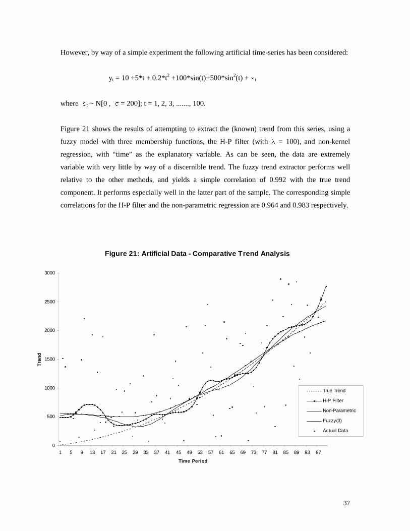
However, by way of a simple experiment the following artificial time-series has been considered:
yt = 10 +5*t + 0.2*t2 +100*sin(t)+500*sin2(t) + Jt
where Jt ~ N[0 , ) = 200]; t = 1, 2, 3, ......., 100.
Figure 21 shows the results of attempting to extract the (known) trend from this series, using a
fuzzy model with three membership functions, the H-P filter (with � = 100), and non-kernel
regression, with “time” as the explanatory variable. As can be seen, the data are extremely
variable with very little by way of a discernible trend. The fuzzy trend extractor performs well
relative to the other methods, and yields a simple correlation of 0.992 with the true trend
component. It performs especially well in the latter part of the sample. The corresponding simple
correlations for the H-P filter and the non-parametric regression are 0.964 and 0.983 respectively.
Figure 21: Artificial Data - Comparative Trend Analysis
0
500
1000
1500
2000
2500
3000
1 5 9 13 17 21 25 29 33 37 41 45 49 53 57 61 65 69 73 77 81 85 89 93 97
Time Period
Tre
nd
True Trend
H-P Filter
Non-Parametric
Fuzzy(3)
Actual Data

38
5.6 Modelling the Demand for Chicken
Our final application is based on an example, and data, provided in Studenmund’s (1997, pp. 174-
175) well known text. This example relates to the demand for chicken, as a function of its own
price, disposable income, and the price of a substitute meat. More specifically, the model is of the
form:
Qt = f(PCt, P
Bt, Yt) + Jt
where:
Q = U.S. per capita chicken consumption (pounds)
PC = U.S. price of chicken (cents/pound)
PB = U.S. price of beef (cents/pound)
Y = natural logarithm of U.S. per capita disposable income (dollars)
The sample (Studenmund, 1997, p.199) comprises annual data for 1951 to 1990 inclusive.
As in the earlier regression examples, we consider OLS, non-parametric kernel estimation, and
fuzzy modelling. The latter is applied to all three (non-constant) explanatory variables. In each
case we use two fuzzy clusters, resulting in 8 potential sub-samples, three of which had positive
degrees of freedom. (Three fuzzy clusters implies 27 potential sub-samples, and this resulted in
only two with positive degrees of freedom. The resulting fuzzy prediction path exhibited erratic
movements at several time-points.)
The basic results are shown in Figure 22 and Table 6. The membership functions were of the
same general form as in the previous examples, and are not shown here to reduce space. As can
be seen in Figure 22, the fuzzy model performs very creditably, and this is reflected in the
%RMSE and %MAE values shown in Table 6. Indeed, if it were not for the relatively poor
predictive performance of the fuzzy model during the period 1974 to 1981, its overall
performance would be exceptionally good. Our view is that the relatively small sample size
disadvantages the fuzzy model in this example, and this may also be an instance where some
experimentation is needed with the value for the exponent parameter, “m”, in the objective
functional for the FCM algorithm.

39
Figure 22: Chicken Consumption Model
-5
5
15
25
35
45
55
65
75
1951
1953
1955
1957
1959
1961
1963
1965
1967
1969
1971
1973
1975
1977
1979
1981
1983
1985
1987
1989
Year
Ch
icke
n C
on
sum
pti
on
(p
ou
nd
s)
Actual
OLS
Non-Parametric
Fuzzy (2)
Figure 23 a: Predicted Own-Price Elasticities
-1.2
-1.0
-0.8
-0.6
-0.4
-0.2
0.0
0.2
0.4
1951
1953
1955
1957
1959
1961
1963
1965
1967
1969
1971
1973
1975
1977
1979
1981
1983
1985
1987
1989
Year
Ow
n-P
rice
Ela
stic
ity
OLS
Non-Parametric
Fuzzy (2)

40
Figure 23 b: Predicted Cross-Price Elasticities
-0.7
-0.5
-0.3
-0.1
0.1
0.3
0.5
0.7
1951
1953
1955
1957
1959
1961
1963
1965
1967
1969
1971
1973
1975
1977
1979
1981
1983
1985
1987
1989
Year
Cro
ss-P
rice
Ela
stic
ity
OLS
Non-Parametric
Fuzzy (2)
Figure 23 c: Predicted Income Elasticities(Multiplied by 1,0000)
-0.5
-0.3
-0.1
0.1
0.3
0.5
0.7
0.9
1.1
1.3
1.5
1.7
1951
1953
1955
1957
1959
1961
1963
1965
1967
1969
1971
1973
1975
1977
1979
1981
1983
1985
1987
1989
Year
Inco
me
Ela
stic
ity(
*100
00)
OLS
Non-Parametric
Fuzzy (2)

41
Table 6: Fuzzy Regression Results for Chicken Consumption Model
(c1 = c2 = c3 = 2; m = 2)
(a) Sub-Model Results*
Fuzzy Cluster Fuzzy Cluster Fuzzy Cluster
Cluster Centre Cluster Centre Cluster Centre
Price of Chicken Price of Beef log(Income)
PC1 10.420 PB1 23.463 Y1 2875.560
PC2 18.166 PB2 60.183 Y2 12175.260
(b) Cluster Intersection Results
Fuzzy Obs. β1 β2 β3 β4
Intersection (t-val.) (t-val.) (t-val.) (t-val.)
(PC1 ∩ PB1 ∩ Y1) 7 to 22, 30.4720 -1.0523 0.2901 0.0026
24 to 27 (9.90) (-5.34) (1.84) (3.70)
(PC1 ∩ PB2 ∩ Y2) 29 to 33, 9.7358 -0.0243 0.3360 0.0024
36 to 38, & 40 (1.42) (-0.07) (4.29) (13.36)
(PC2 ∩ PB2 ∩ Y1) 1 to 6 15.1140 -0.2595 0.1433 0.0061
(0.70) (-0.91) (0.82) (0.58)
(c) Comparative Model Performances**
Least Squares Non-Parametric Fuzzy
%RMSE 5.130 7.692 6.879
%MAE 4.407 6.001 4.559
** β1, β2, β3 and β4 are the coefficients of the intercept, PC, PB, and Y respectively.
* %RMSE = Percent root mean squared error of fit; %MAE = Percent mean absolute error of fit.

42
Figure 23 displays the predicted own-price, cross-price and income elasticities of demand (by
year in the sample) implied by the OLS, non-parametric, and fuzzy models. Those relating to the
non-parametric estimation are quite unsatisfactory. In particular, in each case there are values that
have a sign opposite to that implied by the underlying economic theory. There are no such
aberrations in the case of the fuzzy and OLS results. The latter generally appear somewhat more
plausible as they exhibit fewer marked fluctuations than do the fuzzy elasticities. This weakness
of the fuzzy elasticities is related to a similar feature in the predicted time-paths, noted above in
relation to Figure 22. It is also interesting that the fuzzy income elasticities always exceed those
from OLS estimation, and this is almost always the case with the cross-price elasticities.
5. Concluding Remarks
In this paper we have discussed the possibility of using various analytical tools from fuzzy set
theory and fuzzy logic to model non-linear econometric relationships in a flexible, and essentially
semi-parametric way. More specifically, we have explored the use of the fuzzy c-means
clustering algorithm, in conjunction with the Takagi and Sugeno (1985) approach to fuzzy
systems, in this particular context. The general modelling strategy that we have considered
involves identifying interesting and important fuzzy sets or fuzzy clusters of the multidimensional
data, in a totally non-parametric way; fitting separate parametric regression models to each fuzzy
cluster (or sub-sample) of the data; and then combining the estimates of these separate models in
a very flexible way, based on the “degree of membership” of each sample point to each fuzzy
cluster. It is this last step in the analysis that facilitates the overall procedure’s ability to capture
intrinsic non-linearities, because the “weights” that are effectively assigned to each sub-model
vary continuously from data-point to data-point.
This general fuzzy modelling procedure has a wide range of applications, and we have provided
several empirical applications to illustrate this. Not only can it be used to model and smooth data
in ways that compete directly with established techniques such as non-parametric kernel
regression, or splines, but it can also be used for trend extraction in competition with methods
such as the Hodrick and Prescott (1980, 1997) filter. In all of the cases that we have examined,
the fuzzy modelling approach performs extremely well. Moreover, it has significant practical
advantages over both kernel regression and spline analysis. Spline analysis requires that the
location of the “knots” be known in advance, whereas the first stage of our fuzzy modelling
procedure determines the relevant data groupings empirically. Non-parametric kernel regression

43
suffers from the so-called “curse of dimensionality” that severely limits its application to
relatively simple models. In contrast, the fuzzy modelling structure that we have outlined is
readily applicable to quite complex models, without undue computational burden. Indeed, it
should also be noted that although our illustrative applications have all used ordinary least
squares regression at the second stage of the analysis to fit models to each fuzzy cluster, in fact
any relevant estimation technique could be used at that stage. For instance (and depending on the
context), logit or probit models could be fitted, or non-linear or instrumental variables regression
could be used, without disrupting the general style of the fuzzy modelling strategy that we have
described.
We recognize that the bulk of the discussion in this paper addresses issues relating to curve fitting
and data smoothing, and relatively little attention has been paid to strictly inferential issues. It
was argued heuristically at the end of section 4 that the fuzzy predictor emerging from our
modelling approach will be a (weakly) consistent estimator of the conditional mean of the
dependent variable. While this is minimally helpful, it will hold only under suitable conditions,
and our work in progress explores this issue (and other aspects of the sampling properties of the
fuzzy predictor) more thoroughly.
In this context it is also worth noting that the various “fuzzy predictions” that we have presented
in our examples are simply “point predictions”, and the corresponding confidence intervals are
also extremely important. While it is not immediately clear how straightforward it would be to
construct exact finite-sample prediction intervals within this framework, they could certainly be
approximated by means of bootstrap simulation. Asymptotic prediction intervals can be
constructed relatively easily, as follows. It will be recalled that once the sample has been
partitioned into fuzzy clusters (typically with a different number of data points in each cluster),
our modelling procedure involves estimating a regression over each cluster, and then combining
the results using weights based on the membership values. The precise details are given in “Step
3” in section 4 above. These weights vary continuously, but are exogenous if the regressors also
satisfy this property. Rather than estimate each cluster regression separately, by least squares,
another option is to estimate the group of cluster regressions as a “seemingly unrelated
regressions” (SUR) model. The only complication is that the SUR model is “unbalanced”, in the
sense that the samples associated with each equation are different from one another. However,
unbalanced SUR models can be estimated quite readily (e.g., see Srivastava and Giles, 1987, pp.
339-346, for details). This then provides a complete estimated asymptotic covariance matrix for

44
all of the estimated parameters in all of the cluster regressions. This information (together with
the membership values) can then be used to construct observation-by-observation asymptotic
standard errors for the prediction of the conditional mean of the dependent variable.
By way of illustration we have undertaken this analysis in the case of the earnings-age profile
data analyzed in section 5.1 above, and the results appear in Figure 24. SHAZAM code was
written to produce these results, which are compared with their counterparts from non-parametric
kernel regression. As can be seen, the fuzzy modelling procedure produces intervals that are very
comparable to those from non-parametric regression, in terms of their shape and width. Given
that our illustrative applications are based on relatively small samples, we have not provided
corresponding asymptotic confidence intervals for our other “fuzzy predictions”.
Figure 24: Confidence Intervals for Earnings-Age Profile Predictions
12.4
12.6
12.8
13.0
13.2
13.4
13.6
13.8
14.0
14.2
20 25 30 35 40 45 50 55 60 65
Age
Lo
gar
ith
m o
f E
arn
ing
s
Fuzzy Lower 95%
Fuzzy (3)
Fuzzy Upper 95%
Non-Parametric Lower 95%
Non-Parametric
Non-Parametric Upper 95%

45
Clearly, much remains to be done in order to validate the real worth of the type of “fuzzy
econometric modelling” has been described and illustrated in this paper. None the less, we view
the results presented here as being rather promising. Certainly, further exploration of this
approach to modelling and smoothing non-linear economic data seems to be justified.

46
References
Al-Daoud, M. B. and S. A. Roberts (1996), “New Methods for the Initialisation of Clusters”,
Pattern Recognition Letters, 17, 451-455.
Babu, G. and M. Murty (1993), “A Near-Optimal Initial Seed Value Selection in K-Means
Algorithm Using a Genetic Algorithm”, Pattern Recognition Letters, 14, 763-769.
Bezbek, J. C. (1973), Fuzzy Mathematics in Pattern Classification, Ph.D. Thesis, Applied
Mathematics Center, Cornell University, Ithaca, NY.
Bezbek, J. C. (1981), Pattern Recognition With Fuzzy Objective Function Algorithms, Plenum
Press, New York.
Bishop, C. M. (1995), Neural Networks for Pattern Recognition, Oxford University Press,
Oxford.
Chiu, S. L. (1994), “Fuzzy model Identification Based on Cluster Estimation”, Journal of Fuzzy
and Intelligent Systems, 2, 267-278.
Coppejans, M. (2000), “Breaking the Curse of Dimensionality”, mimeo., Department of
Economics, Duke University.
Cummins, C. (1994), TSP Procedure hptrend44, TSP International,
www.stanford.edu/~clint/tspex/hptrend44.tsp
Dasgupta, M. and R. Deb (1996), “Transitivity and Fuzzy Preferences”, Social Choice and
Welfare, 13, 305-318.
Davé, R. N. (1991), “Characterization and Detection of Noise in Clustering”, Pattern Recognition
Letters, 12, 657-664.
Draeseke, R. and D. E. A. Giles (1999), “A Fuzzy Logic Approach to Modelling the
Underground Economy”, in L. Oxley, F. Scrimgeour and M. McAleer (eds.),
Proceedings of the International Conference on Modelling and Simulation (MODISM
99), Volume 2, Modelling and Simulation Society of Australia and New Zealand,
Hamilton, N.Z., 453-458.
Draeseke, R. and D. E. A. Giles (2000), “A Fuzzy Logic Approach to Modelling the New
Zealand Underground Economy”, forthcoming in Mathematics and Computers in
Simulation.
Dunn, J. C. (1973), “A Fuzzy Relative of the ISODATA Process”, Journal of Cybernetics, 3, 32-
57.
Dunn, J. C. (1974), “Well Separated Clusters and Optimal Fuzzy Partitions”, Journal of
Cybernetics, 4, 95-104.

47
Dunn, J. C. (1977), “Indices of Partition Fuzziness and the Detection of Clusters in Large Data
Sets”, in M. Gupta and G. Seridis (eds.), Fuzzy Automata and Decision Processes,
Elsevier, New York.
Griffiths, W. E., R. C. Hill and G. G. Judge (1993), Learning and Practicing Econometrics,
Wiley, New York.
Frigui, H. and R. Krishnapuram (1996), “A Robust Algorithm for Automatic Extraction of an
Unknown Number of Clusters from Noisy Data”, Pattern Recognition Letters, 17, 1223-
1232.
Hall, B. H. (1996), Time Series Processor Version 4.3, User's Guide, TSP International, Palo Alto
CA.
Heckman and Polachek (1974), “Empirical Evidence on Functional Form of the Earnings-
Schooling Relationship”, Journal of the American Statistical Association, 69, 350-354.
Hsing, Y. and D. J. Smyth (1994), “Kuznets's Inverted-U Hypothesis Revisited”, Applied
Economics Letters, 1, 111-113.
Hodrick, R. J. and E. C. Prescott (1980), “Postwar U.S. Business Cycles: An Empirical
Investigation”, Discussion Paper No. 451, Department of Economics, Carnegie-Mellon
University.
Hodrick, R. J. and E. C. Prescott (1997), “Postwar U.S. Business Cycles: An Empirical
Investigation”, Journal of Money, Credit and Banking, 29, 1-16.
Huang, C. and R. Harris (1993), “A Comparison of Several Vector Quantization Codebook
Generation Approaches”, IEEE Transactions in Image Processing, 2, 108-112.
Jacobsen, P. W. F. and D. E. A. Giles (1998), “Income Distribution in the United States: Kuznets’
Inverted U Hypothesis and Data Non-Stationarity”, Journal of International Trade &
Economic Development, 7, 405-423.
Jolion, J. and A. Rosenfeld (1989), “Cluster Detection in Background Noise”, Pattern
Recognition, 22, 603-607.
Josef, S., G. Korosi and L. Matyas (1992), “A Possible New Approach of Panel Modelling”,
Structural Change and Economic Dynamics, 3, 357-374.
Keller, A. (2000), “Fuzzy Clustering With Outliers”, mimeo., Institute of Flight Guidance,
German Aerospace Center, Braunschweig, Germany.
Kolmogorov, A. N. (1957), “On the Representation of Continuous Functions of Several Variables
by Superpositions of Continuous Functions of One Variable and Addition”, Doklady,
114, 674-681.

48
Kuznets, S. (1955), “Economic Growth and Income Inequality”, American Economic Review, 45,
1-28.
Kydland, F. and E. C. Prescott (1990), “Business Cycles: Real facts and a Monetary Myth”,
Federal Reserve Bank of Minneapolis Quarterly Review, Spring, 3-18.
Linde, Y., A. Buzo and R. Gray (1980), “An Algorithm for Vector Quantizer Design”, IEEE
Transactions in Communication, 28, 84-95.
LindstrCm, T. (1998), “A Fuzzy Design of the Willingness to Invest in Sweden”, Journal of
Economic Behaviour and Organization 36, 1-17.
Lorentz, G. G. (1966), Approximation of Functions, Holt, Rinehart and Winston, New York.
Lott, W. F. and S. C. Ray (1992), Applied Econometrics: Problems With Data Sets, Dryden Press,
New York.
MacQueen, J. (1967), “Some Methods for Classification and Analysis of Multivariate
Observations”, in J. M. Le Cam and J. Neyman (eds.), Proceedings of the 5th Berkeley
Symposium in Mathematical Statistics and Probability, University of California Press,
Berkeley CA, 281-297.
Mincer, J. (1974), Schooling, Experience and Earnings, Columbia University Press for the
National Bureau of Economic Research, New York.
Murphy, K. M. and F. Welsch (1990), “Empirical Age-Earnings Profiles”, Journal of Labor
Economics, 8, 202-229.
Pagan, A. and A. Ullah (1999), Nonparametric Econometrics, Cambridge University Press,
Cambridge.
Richardson, G. (1998), “The Structure of Fuzzy Preferences: Social Choice Implications”, Social
Choice and Welfare, 15, 359-369.
Ruspini, E. (1970), “Numerical Methods for Fuzzy Clustering”, Information Science, 2, 319-350.
Sengupta, K. (1999), “Choice Rules With Fuzzy Preferences: Some Characterizations”, Social
Choice and Welfare, 16, 259-272.
SHAZAM (2000), SHAZAM Econometrics Software: User's Reference Manual Version 9,
SHAZAM Econometrics Software, Vancouver B.C.
Shepherd, D. and F. K. C. Shi (1998), “Economic Modelling With Fuzzy Logic”, paper presented
at the CEFES ’98 Conference, Cambridge, U.K..
Silverman, B. W. (1986), Density Estimation for Statistics and Data Analysis, Chapman and Hall,
London.

49
Singh, R. S., A. Ullah and R. A. L. Carter (1987), “Nonparametric Inference in Econometrics:
New Applications”, in I. A. MacNeil and G. J. Umphrey (eds.), Time Series and
Econometric Modelling, Vol. III, Reidell, Boston MA.
Srivastava, V. K. and D. E. A. Giles (1987), Seemingly Unrelated Regression Equations Models:
Estimation and Inference, Marcel Dekker, New York.
Studenmund, A. H. (1997), Using Econometrics: A Practical Guide, 3rd. ed., Addison-Wesley,
Reading, MA.
Sugeno, M. and G. T. Kang (1985), “Structure Identification of a Fuzzy Model”, Fuzzy Sets and
Systems, 28, 15-33.
Takagi, T. And M. Sugeno (1985), “Fuzzy Identification of Systems and its Application to
Modelling and Control”, IEEE Transactions on Systems, Man and Cybernetics, 15, 116-
132.
Tou, J. and R. Gonzales (1974), Pattern Recognition Principles, Addison-Wesley, Reading MA.
Ullah, A. (1985), “Specification Analysis of Econometric Models”, Journal of Quantitative
Economics, 1, 187-209.
U.S. Department of Commerce (2000), U.S. Real Personal Consumption Expenditures, monthly,
seasonally adjusted at annual rates, billions of chained 1996 dollars, downloaded from
FRED database at URL www.stls.frb.org/fred/data/gdp/pcec96 on 14 August, 2000;
U.S. Real Disposable Personal Income, monthly, seasonally adjusted at annual rates,
billions of chained 1996 dollars, downloaded from FRED database at URL
www.stls.frb.org/fred/data/gdp/dspic96 on 14 August, 2000.
U.S. Department of Commerce (various years), Economic Report of the President.
Akkeren, M. (2001), “Computationally Intensive Methods for Deriving Optimal Trimming
Parameters”, forthcoming in D. E. A. Giles (ed.), Computer-Aided Econometrics, Marcel
Dekker, New York.
Weiss, I. (1988), “Straight Line Fitting in a Noisy Image”, Proceedings in Computer Vision and
Pattern Recognition, 647-652.
White, H. (1992), Artificial Neural Networks: Approximation and Learning Theory, Blackwell,
Cambridge, MA.
White, H., and A. R. Gallant, (1992), “On Learning the Derivatives of an Unknown Mapping
with Multilayer Feedforward Networks”, Neural Networks, 5, 129-138.
Yager, R. R. and D. P. Filev (1992), “Learning of Fuzzy Rules by Mountain Clustering”,
Proceedings of the SPIE Conference on Applications of Fuzzy Logic Technology, Boston
MA, 246-254.

50
Zadeh, L. A. (1965), “Fuzzy Sets”, Information and Control, 8, 338-353.
Zadeh, L. A. (1987), Fuzzy Sets and Applications: Selected Papers, Wiley, New York.