Econometric Modeling of Financial Time Series Volatility ...ceur-ws.org/Vol-1844/10000056.pdf ·...
16
Econometric Modeling of Financial Time Series Volatility Using Software Packages Olena Liashenko 1 , Tetyana Kravets 1 , Kateryna Krytsun 1 1 Taras Shevchenko National University of Kyiv [email protected], [email protected], [email protected] Abstract. The article is devoted to the comparative analysis of software packages in financial time series modeling. The most common among economists packages R, Eviews and Gretl are considered. Volatility is often used as a rough approximation to measuring of overall risk financial instru- ments. Polish stock index WIG for the modeling of financial time series vola- tility was chosen. Econometric model of family GARCH describing the volatility of financial time series is built by means of these packages. Advantages and disadvantages of each software are considered. Keywords. GARCH model, stock indices, volatility, modelling Key Terms. Model, Research, Specification Process 1 Introduction The great achievement of mankind is the development of science and technology. Computing operations require much less efforts of researcher thanks to modern computer technology. Today IT sector is developing rapidly. The results of its activities are the funds of multiplying income, reduce the cost of resources, facilitate professional activity. Information technology facilitates the research process. Analysis of the vast amount of data is possible due to modern software packages. These software products enable to analyze and to model the time series dynamics, to search interdependencies of the time series. The research of stock indices dynamics and stock prices is an important problem in the investment portfolio management. Stock market indices are the indicators of the global economy, group of countries or national economy, investment climate in the country, tools of analysis of securities market and its forecasting trends. In addition, stock index is also independent financial instrument to hedge the securities market. Typically, absolute index values are not so important for investors as its dynamics,
Transcript of Econometric Modeling of Financial Time Series Volatility ...ceur-ws.org/Vol-1844/10000056.pdf ·...

Econometric Modeling of Financial Time Series Volatility
Using Software Packages
Olena Liashenko1, Tetyana Kravets1, Kateryna Krytsun1
1 Taras Shevchenko National University of Kyiv
[email protected], [email protected],
Abstract. The article is devoted to the comparative analysis of software
packages in financial time series modeling. The most common among
economists packages R, Eviews and Gretl are considered. Volatility is often
used as a rough approximation to measuring of overall risk financial instru-
ments. Polish stock index WIG for the modeling of financial time series vola-
tility was chosen. Econometric model of family GARCH describing the
volatility of financial time series is built by means of these packages.
Advantages and disadvantages of each software are considered.
Keywords. GARCH model, stock indices, volatility, modelling
Key Terms. Model, Research, Specification Process
1 Introduction
The great achievement of mankind is the development of science and technology.
Computing operations require much less efforts of researcher thanks to modern
computer technology. Today IT sector is developing rapidly. The results of its
activities are the funds of multiplying income, reduce the cost of resources, facilitate
professional activity.
Information technology facilitates the research process. Analysis of the vast
amount of data is possible due to modern software packages. These software products
enable to analyze and to model the time series dynamics, to search interdependencies
of the time series.
The research of stock indices dynamics and stock prices is an important problem in
the investment portfolio management. Stock market indices are the indicators of the
global economy, group of countries or national economy, investment climate in the
country, tools of analysis of securities market and its forecasting trends. In addition,
stock index is also independent financial instrument to hedge the securities market.
Typically, absolute index values are not so important for investors as its dynamics,
which you can use to determine the direction of the stock market dynamics. Analyti-
cal agencies and stock exchanges calculate Stock Indices.
The aim of the article is an analysis of software that is popular among economists
and modeling of financial time series volatility using software packages R, Gretl,
Eviews.
Software R is the most popular tool among economists, Eviews occupies the sec-
ond position. The package Gretl is not so widespread and powerful. However Gretl
has the ability to use scripts R, Octave, Python etc. Functions package Gretl is ap-
pended by users and it is gaining popularity gradually.
2 Analysis of Recent Research
Modeling and forecasting of time series volatility in financial markets is an urgent
problem for investment advisors, economists and other professionals. Therefore, a
large number of scientific papers are devoted to this sphere. Thus, Subbotin [1] inves-
tigates the main approaches to modeling the volatility of shares and exchange rates,
and reviews the cascade of volatility models in multiple horizons.
Leucht, Kreiss, Neumann [2] suggest the specification test for consistent
generalized autoregressive conditional heteroskedasticity model (GARCH (1,1)),
based on the Cramer-Mises test statistics in their paper.
Barunik, Krehlik, Vacha [3] propose an improved approach to the volatility model-
ing and forecasting using high-frequency data. The model of forecasting based on
Realized GARCH with multiple time-frequency data is used.
Harvey and Lange [4] propose an updated and expanded ARCH in Mean model.
EGARCH-M model, which is displayed in the paper, is useful theoretically and prac-
tically. This model expansion allows distinguishing long and short effects of return to
the volatility.
The global financial crisis of 2008-2009 has raised new questions about the rela-
tionship between investment funds and stock market returns. Therefore, Babalos,
Caporale and Spagnolo [5] analyze US monthly data for the period 2000:1-2015:08.
Authors estimate VAR-GARCH(1,1)-in-mean model with a BEKK and the switch as
a dummy variable, which is necessary to display the global financial crisis. The rela-
tionship between the yield of the stock market and direct investment flows fund is
investigated. It was found that such relationship is weakened during the crisis.
3 Research Method
One of the characteristics of financial markets is the uncertainty that changes over
time. In this regard, there is such a thing as "volatility clustering". It means that the
volatility varies periodically, i.e. stock index dynamics changes from slightly chang-
ing to more chaotic. It's worth to note that many financial relationships are nonlinear internally. It dealt
with peculiarities of financial data, such as the tendency of financial time series (e.g.,
income on assets) to have an unusual distribution of critical areas ("tails") and dis-

placements to the average (leptokurtosis). In addition, often financial time series
change by clusters or pools (volatility clustering or volatility pooling), while larger
deviation of time series prior to high deviation, low deviation of time series - minor
deviations (regardless of sign). It is also possible the leverage effect, i.e. the tendency
to volatility increasing not of the growth but the fall of certain financial and economic
indicators (information asymmetry). Overall volatility modeling and forecasting in the
stock market became a priority for both theoretical and applied research in recent
years. Volatility, as measured by standard deviation or variance of return (such as
securities) is often used as a rough approximation to measuring of overall risk finan-
cial instruments (securities).
The measure of volatility is a variance of series. ARIMA model can not adequately
take into account the inherent characteristics for financial time series. Therefore, there
is a need to use other tools. One of them is ARCH-processes (Autoregressive Condi-
tional Heteroskedasticity). The first such expansion of regression models was present-
ed by Engle [6], after that numerous modifications of the basic design and examples
of the new model for financial and macroeconomic time series were developed. First,
ARCH-models studied inflation uncertainty. Later, they were used in the volatility
analysis of prices and yields of speculative assets. On the basis of applying ARCH-
models it was found that the dynamics of volatility for many financial variables sub-
ject to stable laws.
ARCH/GARCH models belong to the class of nonlinear models of conditional var-
iance, which changes over time. This allows, in addition to the average value of the
studied parameters, to model the dynamics of its variance simultaneously. Therefore,
such model can correctly describe phenomena such as clustering of volatility, asym-
metric information, etc.
Examples of financial time series with high frequency are stock prices and indices
of commodity exchanges. In practical researches they are often analyzed in the form
of geometric income, i.e. the logarithm of the rate of increase in the price of an asset
(or rate of stock index growth) ty :
1
1
log log log ,tt t t
t
yr y y
y
(1)
where tr – geometric income of the asset. ARCH-extension model is the GARCH-model volatility, where the current volatili-
ty affects both preceding price changes and preceding volatility estimates (so-called
"old news"). Memory of ARCH(q)-process is limited by q-periods. We need long lag
q and a large number of parameters for using models. Generalized ARCH-process
(Generalized ARCH or GARCH), proposed by Bollerslev [7], has infinite memory
and allows more economical parameterization.
Overall, ARCH/GARCH methodology can be described as studied parameters dis-
persion modeling methodology. Since the variance is second-order moment, the dis-
persion model is nonlinear. Therefore, it can not be evaluated by the methods devel-
oped for linear models, particularly using ARIMA models. Autoregressive conditional

heteroskedasticity, i.e. the change of random variables (disturbances) variance in the
time, formalized represented as:
1 1 1 2 3, , ,..., ,t t y ta y y y y y (2)
where 1ta – perturbations (random variable) at time period (t+1),
1ty – value at time period (t+1),
1 2 3, , ,...,y ty y y y – mean value estimated on the basis of data that preceded the
moment (t+1).
Dispersion equation in GARCH models unlike ARCH models takes into account
variables other than lagged random variables, and more variables lagged conditional
variance. Actually overall ARCH/GARCH model can be presented as a series of fil-
ters.
Note that the smoothing procedure or seasonal deprivation for time series are
optional and executed as needed. Overall, ARCH/GARCH model can be considered
as "supplement" for a multi-linear regression and ARIMA models. Evaluation of
ACRH/GARCH models can not be implemented by the method of least squares.
Special procedures developed for evaluation of these models, including maximum
likelihood method.
4 Results
According to the Bloomberg Businessweek, 97 percent of companies in Fortune
500 have used business analytics and some forms of Big Data analytics to conduct
their business. Big Data analytics that processes data into information and particularly
knowledge has emerged as a contemporary business trend in industry and academics
[8]. Many consultants, scientists, and researchers pay attention to Big Data because it
contains meaningful information. Various applications such as healthcare, security,
medicine, politics, etc. can use the information to solve data-related problems in soci-
ety.
One of the most dominant analytics tools in Big Data Analytics is the R Project, or
R. R is a general statistical analysis platform that runs on the command line. It is
world’s most widely used, open-source statistical programming language designed for
friendly use.
Other popular packages are Eviews and Gretl. Here is a comparative description of
these software packages (Table 1).
Features in Gretl [9].
1. Easy intuitive interface.
2. A wide variety of estimators: least squares, maximum likelihood, GMM; single-
equation and system methods.

3. Time series methods: ARIMA, a wide variety of univariate GARCH-type models,
VARs and VECMs (including structural VARs), unit-root and cointegration tests,
Kalman filter, etc.
4. Limited dependent variables: logit, probit, tobit, sample selection, interval regres-
sion, models for count and duration data, etc.
5. Panel-data estimators, including instrumental variables, probit and GMM-based
dynamic panel models.
6. Output models as LaTeX files, in tabular or equation format.
7. Integrated powerful scripting language (known as hansl), with a wide range of
programming tools and matrix operations.
8. GUI controller for fine-tuning Gnuplot graphs.
9. An expanding range of contributed function packages, written in hansl.
10. Facilities for easy exchange of data and results with GNU R, GNU Octave, Py-
thon, Ox and Stata.
Table 1. Comparative description of data analysis software packages
Features Eviews Gretl R
Data extensions *.wf1 *.gdt, *.gdtb *.R
User interface Mostly point-
and-click
Scripting/point and
click
Programming
Data manipulation Strong Strong Very strong
Data analysis Powerful Powerful Powerful/versatile
Graphics Good Good Excellent
Cost Expensive, but
has free student
lite version
Open source Open source
Output extensions *.wf1 CSV, gdt, gdtb,
GNU R, Octave,
Stata, JMulTi,
PcGive
*R, *.txt(log files,
any word processor
can read)
Features in Eviews [10].
1. Integrated support for handling dates and time series dat.
2. Support for high-frequency (intraday) data, allowing for hours, minutes, and sec-
onds frequencies. In addition, there are a number of less commonly encountered
regular frequencies, including Multi-year, Bimonthly, Fortnight, Ten-Day, and
Daily with an arbitrary range of days of the week.
3. Long-run variance and covariance calculation: symmetric or one-sided long-run
covariances using nonparametric kernel (Newey-West 1987, Andrews 1991), par-
ametric VARHAC (Den Haan and Levin 1997), and prewhitened kernel (Andrews
and Monahan 1992) methods. In addition, EViews supports Andrews (1991) and
Newey-West (1994) automatic bandwidth selection methods for kernel estimators,

and information criteria based lag length selection methods for VARHAC and
prewhitening estimation.
4. Linear quantile regression and least absolute deviations (LAD), including both
Huber’s Sandwich and bootstrapping covariance calculations.
5. Stepwise regression with seven different selection procedures.
6. Threshold regression including TAR and SETAR.
7. Heckman Selection models.
8. Object-oriented command language provides access to menu items.
9. Batch execution of commands in program files.
10. String and string vector objects for string processing. Extensive library of string
and string list functions.
Features in R [11].
1. R is free, open-source software distributed and maintained by R-project, R source
code is available under the Free Software Foundation’s GNU General Public Li-
cense.
2. R supports most of the data analysis techniques such as virtual data manipulation,
statistical model, and charts.
3. R support beautiful and unique data visualizations to present multidimensional da-
ta in multi-panel charts, 3-D graphs.
4. A global R community of 2 million users, developers, and contributors support
contribute and maintain R language. Revolution Analytics community was ac-
quired by Microsoft.
5. Provides better results faster than legacy statistical software’s counterpart does.
6. R has data structures (vectors, matrices, arrays, data frames) that users can operate
on through functions for performing statistical analyzes and creating graphs.
7. Object-oriented programming: C, Java, Perl, Python, parallel programming, etc.
8. Applications: Chemometrics, Clinical trial, Econometrics, Medical images, etc.
9. Data Mining and Machine Learning: Arules, Cubist, knnTree, randomFores, etc.
10. Statistical methodology: Bayesian inference, Spatial data, Time Series, etc.
In summary, the paper defined Big Data, compared and contrasted the statistical
features of R to its programming features and its relevance. It provided the primary
programming features available in R and described how the analytics software tool R
was suited for Big Data today [11].
Polish stock index WIG for the modeling of financial time series volatility was
chosen. The data obtained from the Google Finance site [12]. The results of volatility
modeling for the stock index WIG in software packages R, Eviews, Gretl are com-
pared.
First of all we analyze time series data for normality of distribution, define the
asymmetry and kurtosis. The package R uses a series of commands and obtain the
following numerical characteristics:
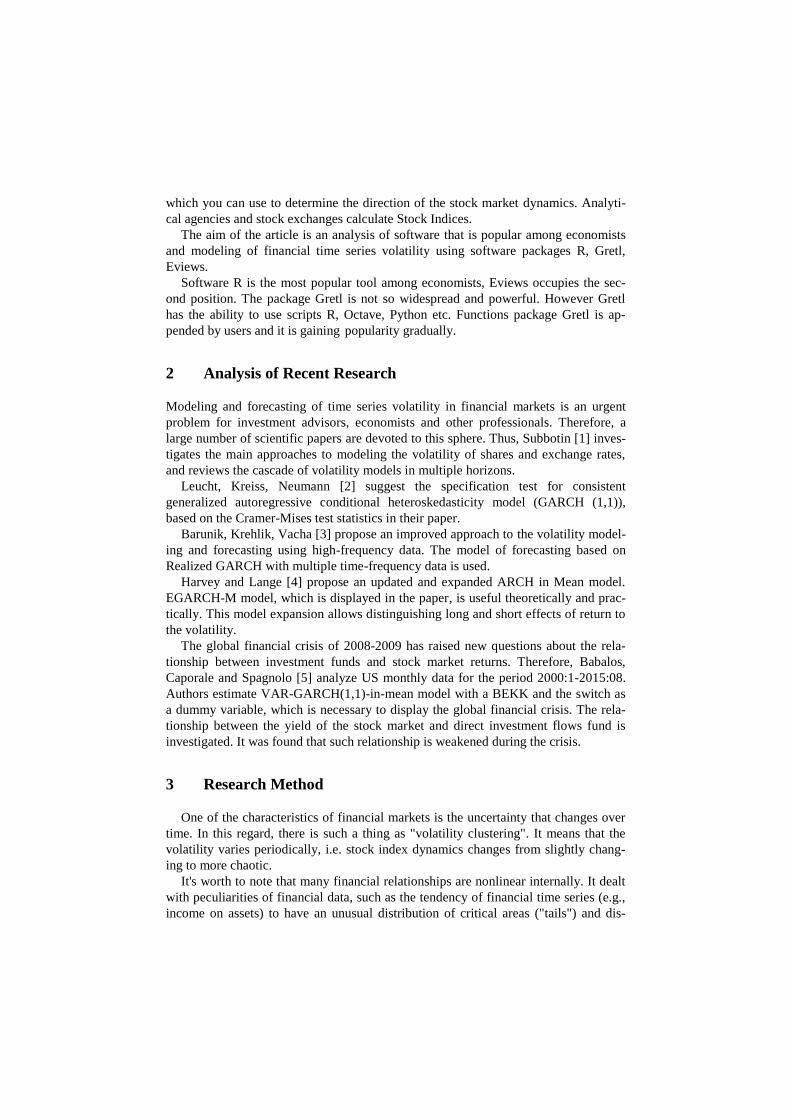
> skewness(wr)
[1] -0.4892253
> kurtosis(wr)
[1] 3.844628
> mean(wr)
[1] 0.03569432
Asymmetry is -0.4892253, which means that the distribution of data is skewed
slightly to the left. We have 3.844628 for excess, that is greater than 3, and therefore,
the distribution is leptokurtic. Fig. 1 shows the density of index WIG yield (2004-
2016 daily), which is asymmetric and leptokurtic.
Fig. 1. Distribution density of index WIG yield in R
In Eviews software package it is much easier to conduct a preliminary analysis of
time series, for pressing a sequence of buttons View-Descriptive Statistics… - Histo-
gram and Stats we obtain simultaneous display table of distribution and numerical
characteristics (Fig. 2).
In the software package Gretl we need to make a few clicks to display the graph
and numerical characteristics of series or write a script. The results of these actions
are presented in Figure 3. Herewith Skewness = -0.48944, Кurtosis = 3.8487.
In all software package kurtosis and skewness do not differ significantly, but aver-
age values are equal.
The next step is to analyze the yield graph to identify the phenomenon of clustering
and analysis of autocorrelation and partial autocorrelation for time series. The pack-
age R should use the command: tsdisplay(wig$wig_return) to display graphics and
return of time series.
Fig. 4 shows the results of this command. Graph of yield has signs of clustering.
There is also residual autocorrelation. Graphs of autocorrelation function (ACF) and
partial autocorrelation residues (PACF) show strong visible emissions for the first
order lagged values indicating the feasibility of using GARCH(1,1).

Fig. 2. Distribution density of index WIG yield in Eviews
0
0.05
0.1
0.15
0.2
-8 -6 -4 -2 0 2 4 6
Rel
ativ
e fr
equen
cy
wig_return Fig. 3. Distribution density of index WIG yield in Gretl
Fig. 4. The graphs of WIG return, autocorrelation function and partial autocorrelation residues
function in R

According to the software packages Eviews and Gretl we can do this in a few
clicks. It is noticeable that received graphic display is identical (Fig. 5, 6).
However, according to the fig. 6 it is hard to understand when autocorrelation resi-
dues present, and we can be argued that there is autocorrelation residues to 36 order
(lag) given the probability value (Prob.). Therefore, for the analysis of residual auto-
correlation and time series clustering the best software packages are R and Gretl.
-0.1
-0.05
0
0.05
0.1
0 5 10 15 20 25 30 35
lag
ACF for wig_return
+- 1.96/T^0.5
-0.1
-0.05
0
0.05
0.1
0 5 10 15 20 25 30 35
lag
PACF for wig_return
+- 1.96/T^0.5
Fig. 5. The graphs of autocorrelation function and partial autocorrelation residues function of
WIG returns in Gretl
We turn to the construction of model and its specification. To select the best
models in R, its testing and forecasting should prescribe following code:
spec <- ugarchspec()
fit = ugarchfit(data = wr, spec = spec, out.sample =
3000)
show(fit)
forc = ugarchforecast(fit, n.ahead=100, n.roll = 100)
forc
plot(forc, which = "all")
As a result of the code, we received the best model GARCH(1,1) and model for
average ARMA(1,1). Optimal parameters of the model GARCH(1,1) are presented in
the Table 2, information criteria of the model are given in the Table 3.

Table 2. GARCH(1,1) optimal parameters
Estimate Std. Er-
ror
t value Pr(>|t|)
Mu 0.154131 0.052193 2.953101 0.003146
ar1 -0.683459 0.153773 -4.444588 0.000009
ma1 0.780920 0.129864 6.013347 0.000000
omega 0.000085 0.007050 0.012009 0.990418
alpha1 0.049252 0.015846 3.108058 0.001883
beta1 0.949748 0.017353 54.729664 0.000000
According to the t-statistics, which probability value indicates the significance of
the model parameters, we obtained omega only as insignificant factor. Wherein the
information criteria are not high, therefore the model is well constructed.
Table 3. Information criteria of the model
Akaike 2.9394
Bayes 3.0038
Shibata 2.9389
Hannan-Quinn 2.9650
So, we specify GARCH(1,1) in Gretl and Eviews similarly. In the package gig.gfn
one has the opportunity to evaluate various options of GARCH family models and to
add ARMA model for average. In the process of the model constructing, it was found
that adding lag for AR automatically added lag for MA, due to the fact that the adding
of AR(1) only the model will be not identified. The results are shown in Fig. 6.
Fig. 6. Model GARCH(1,1) AR(1)

All parameters of the model are significant, but the value of information criteria are
high compared with those calculated in R. Gig.gfn package does not allow to check
ARCH-effects or autocorrelation stability parameters of the model.
The package Gretl doesn’t make possible to check the model ARCH-effects or au-
tocorrelation stability parameters. You can build a forecast and graphics in this pack-
age.
If you use standard functional (basic), which is immediately available after in-
stalling the software package Gretl, it provides an estimate normal GARCH model,
which results are shown in Fig. 7.
Fig. 7. GARCH(1,1) in Gretl
Compared with functional package gig.gfn, the basic functional of Gretl allows
you to conduct more tests of the results. However, just three tests of the list are avail-
able in the tests menu.
Perform forecasting for two GARCH models were built in Gretl. Under the first
model, which is shown in Fig. 8, forecast of 100 observations (days) has received.
From Fig. 8 it can be seen that the dynamics of the conditional variance will increase.
This shows the impact of negative news in the market and the presence of asymmetry,
so you should apply the model of GARCH family, which takes into account the
asymmetries in the market, namely EGARCH model.
Fig. 9 shows the projected range of volatility fluctuation. According to the forecast
the WIG return volatility will increase gradually over the forecast period and will
increase by almost half.
We proceed to the construction of GARCH(1,1), ARMA(1,1) models in the soft-
ware package Eviews 9.5 Student's version Lite. Simulation results are presented in
Fig. 10.

0.5
1
1.5
2
2.5
3
0 10 20 30 40 50 60 70 80
conditio
nal variance f
or
wig
_re
turn
GARCH(1,1) [Bollerslev]
Fig. 8. Forecasting of conditional variance for WIG return volatility in gig.gfn
-5
-4
-3
-2
-1
0
1
2
3
2016.4 2016.5 2016.6 2016.7 2016.8 2016.9 2017 2017.1
95 percent interval
wig_return
forecast
Fig. 9. Forecasting of WIG return volatility (the basic functional of Gretl)
The sum of the regression coefficients expresses the impact of variables variance
prior period to the current value of the variance. This value is close to 1, which is a
sign of the growing inertia effect of shocks on variance of financial assets returns.
According to Durbin-Watson statistics the residual autocorrelation is absent, most
coefficients of the model are significant. For Inverted ARMA Roots the parameters
ARMA(1,1) are stable because they are smaller than 1.
Fig. 11 displays the results of checking ARCH-effects. In this model ARCH-
effects are absent that is positive for the constructed model. The package allows the
testing of the model in squares residual autocorrelation test using Q-statistics. The
lack of residual autocorrelation to 36-th lag allows to include regression for the aver-
age as ARMA(1,1).

Fig. 10. Statistics of GARCH(1,1) model with ARMA(1,1) in Eviews
Fig. 11. The test for the presence of ARCH-effects in Eviews
Note that the GARCH(1,1) model building in Eviews and Gretl software packages
is complicated process because of the inclusion of ARMA(1,1) model for average.
However, the results of obtained model in Eviews and its statistics are more visible.
The advantage of the software package R is that writing a few lines of code, you can
get statistic models, options, and all necessary tests to check for correct specification.
The key tests for GARCH models in software packages Eviews and Gretl are limited
compared with the R. In order to detect, for example, the presence of the effect of
leverage you should further evaluate other family of GARCH model and analyze the
resulting statistics and conduct tests again.
Let us compare the results of forecasts obtained by Gretl, R and Eviews software
products. We received the forecast of conditional variance for WIG return volatility,
and the forecast of WIG return volatility (Fig. 8, 9) in gig.gfn additionally installed
package and Gretl basic functional.
The package R received several graphic maps expectations. In Figure 12 we pre-
sent the results of forecasting time series of absolute dispersion, forecasting real time
series data with conventional variance, forecasting unconditional variance and fore-
casting Rolling Sigma from time series.

Fig. 12. Forecasting of WIG return volatility in R
Note that the dynamics of unconditional variance has a downward trend. This vol-
atility of the time series will fluctuate at the same level of low growth.
In Eviews static and dynamic forecasts of volatility and variance of time series
with numerical forecast forward 43 observations (Fig. 13, 14) can be built.
Note that the forecasts in Eviews are difficult to interpret. However, the volatility
of dynamic forecast tends to increase. As for static forecast, the volatility of the time
series will fluctuate around the same level.
Fig. 13. Dynamic forecasting of WIG return volatility and variance in Eviews

Fig. 14. Static forecasting of WIG return volatility and variance in Eviews
5 Conclusions
It can be concluded that Gretl, Eviews and R can model and forecast the volatility
of financial time series, such as stock indexes. However, using an additional package
gig.gfn it is worth to specify several models e.g. EGARCH or TGARCH models.
The kind of econometric analysis intended to use need to be considered while the
choosing an appropriate package. R should be used for more advanced work, for ex-
ample, to simulate economic models. Gretl and R have the significant advantage as
they are generally available. Gretl basic package is complete and covers most applica-
tions time series and panel data. Add-ons that extend the functional include seasonal
smoothing.
In our opinion, R together with R-studio is the best software package for modeling
the volatility of financial time series. For educational purposes Eviews or Gretl should
be used. Gretl is more flexible and free, extremely easy to use, unlike other software,
therefore it is better to be used in educational institutions.
References
1. Subbotin, A.V.: Volatility Models: from Conditional Heteroscedasticity to Cascades at
Multiple Horizons. Applied Econometrics, 15(3), 94-138 (2009)
2. Leucht, A., Kreiss, J.-P., Neumann, M.H.: A Model Specification Test for GARCH(1,1)
Processes. Scandinavian Journal of Statistics, 42(4) (2015)
3. Barunik, J., Krehlik, T., Vacha, L.: Modelling and forecasting exchange rate volatility in
time-frequency domain. https://arxiv.org/pdf/1204.1452.pdf
4. Harvey, A., Lange, R.-J.: Modeling the Interactions between Volatility and Returns. Cam-
bridge Working Papers in Economics. CWPE 1518.
http://www.econ.cam.ac.uk/research/repec/cam/pdf/cwpe1518.pdf

5. Babalos, V., Caporale, G.M., Spagnolo, N.: Equity Fund Flows and Stock Market Returns
in the US before and after the Global Financial Crisis: A VAR-GARCH-in-mean Analysis.
Economics and Finance Working Paper Series. Working Paper No. 16-12. June 2016.
Brunel University London Department of Economics and Finance.
https://www.brunel.ac.uk/__data/assets/pdf_file/0009/478314/1612.pdf
6. Engle, R.: Autoregressive Conditional Heteroscedasticity with Estamates of the Variance
of United Kingdom Inflation. Econometrica, 50(4), 987-1008 (1982)
7. Bollerslev, T.: Generalized Autoregressive Conditional Heteroskedasticity. Journal of
Econometrics, 31, 307-327 (1986)
8. Minelli, M., Chambers, M., Dhiraj, A.: Big Data Technology, in Big Data, Big Analytics:
Emerging Business Intelligence and Analytic Trends for Today's Businesses, John Wiley
& Sons, Inc. (2013)
9. Gnu Regression Econometrics and Time-series Library. http://gretl.sourceforge.net/
10. Eviews 9.5 Feature List. http://www.eviews.com/EViews9/ev9features.html
11. Le, T.S.: Statistical&Programming Features of R.
https://www.linkedin.com/pulse/statistical-programming-features-r-thiensi-le
12. Google Finance.
https://www.google.com/finance/historical?q=WSE:WIG&ei=98ZNU6CMMMPJsQfdOQ
13. Ghalanos, A.: Introduction to the rugarch package. (2015). https://cran.r-
project.org/web/packages/rugarch/vignettes/Introduction_to_the_rugarch_package.pdf
14. Vasudevan, R. D., Vetrivel, S. C.: Forecasting Stock Market Volatility using GARCH
Models: Evidence from the Indian Stock Market. Asian Jourmal of Research in Social Sci-
ences and Humanities, 6(8), 1565-1574 (2016).
15. Liboschik, T. , Fokianos, K., Fried, R.: tscount: An R Package for Analysis of Count Time
Series Following Generalized Linear Models / Vignette of R package tscount version 1.3.0
(2015).
16. Chiu, C.-W. (J.), Harris, R., Stoja, E., Chin, M.: Financial market volatility,
macroeconomic fundamentals and investor sentiment. Bank of England. Staff Working
Paper, 608 (2016).
17. AL-Najjar, D.: Modelling and Estimation of Volatility Using ARCH/GARCH Models in
Jordan’s Stock Market. Asian Journal of Finance&Accounting, 8(1) (2016).
18. Innocent, N., Mung’atu, J. K.: Modeling Time-Varying Variance-Covariance for Exchange
Rate Using Multivariate GARCH Model. International Journal of Thesis Projects and Dis-
sertations, 4(2) (2016).
19. Spulbar, C., Nitoi, M.: The Impact Of Political And Economic News On The EURO/RON
Exchange Rate: A GARCH Approach. Annals of the „Constantin Brâncuşi” University of
Târgu Jiu, Economy Series, 4, 52-58 (2012)