1

ECONOMETRIC EVALUATION OF THE SEWA BANK IN INDIA

APPLYING MATCHING TECHNIQUES BASED ON

THE PROPENSITY SCORE

Britta Augsburg

Working paper MGSoG/2008/WP004

July 2006 (Revised Version)

Maastricht UniversityMaastricht Graduate School of Governance

2

Maastricht Graduate School of Governance

The 'watch dog' role of the media, the impact of migration processes, health careaccess for children in developing countries, mitigation of the effects of GlobalWarming are typical examples of governance issues – issues to be tackled at thebase; issues to be solved by creating and implementing effective policy.

The Maastricht Graduate School of Governance, Maastricht University, preparesstudents to pave the road for innovative policy developments in Europe and the worldtoday.

Our master's and PhD programmes train you in analysing, monitoring and evaluatingpublic policy in order to strengthen democratic governance in domestic andinternational organisations. The School carefully crafts its training activities to givenational and international organisations, scholars and professionals the tools needed toharness the strengths of changing organisations and solve today’s challenges, and moreimportantly, the ones of tomorrow.

AuthorsBritta Augsburg, PhD fellowMaastricht Graduate School of GovernanceMaastricht UniversityEmail: britta.augsburgunimaas.nlSee also 2006WP003

Mailing addressUniversiteit MaastrichtMaastricht Graduate School of GovernanceP.O. Box 6166200 MD MaastrichtThe Netherlands

Visiting addressKapoenstraat 2, 6211 KW MaastrichtPhone: +31 43 3884650Fax: +31 43 3884864Email: info-gov@governance.unimaas.nl

3

ECONOMETRIC EVALUATION OF THE SEWA BANK IN INDIA

- APPLYING MATCHING TECHNIQUES BASED ON THE PROPENSITY SCORE -

ABSTRACT

This study assesses whether the microfinance institution SEWA Bank, India, is meeting itsobjective of raising its members' income. A cross-sectional analysis is undertaken to assess theoverall income effect of being a member as well and the effect of being a first-time ascompared to repeat borrower. Results suggest that while being a member has a positive andsignificant effect on income, taking a first loan does not. The latter finding is stressed in alongitudinal setting, applying Difference-in-Differences techniques. The effect of taking a firstloan is estimated to be negative and highly insignificant. This confirms the hypothesis thatpositive effects of microfinance are not a matter of shortterm interventions.

ACKNOWLEDGMENTS

I would like to thank my supervisors Prof. Jean-Pierre Urbain, Prof. Pierre Mohnen and Denisde Crombrugghe for their input and interest, Ewa Slowinska and discussants at conferences,namely Robert Sparrow at the Development Economics Seminar, Maastricht 2006 and Dr.Pamela Krishnan, Dr. Sylvie Lambert and Dr. Amad K. Basu at the EUDN workshop in Bonn2006 and finally Armando Barrientos for very useful comments.

4

1. INTRODUCTION

This study assesses whether the microfinance institution SEWA Bank in Ahmedabad, India, a

sister institution of the Self Employed Women's Association, is meeting one of its targeted ten

point objectives: raising their members' income.i The data used in the analysis stems from

surveys conducted in 1998 and 2000 by Harvard University researchers in close collaboration

with a team of the Taleem Research Foundation, an Ahmedabad-based research firm. It

provides a panel of 798 respondents, split up in members of SEWA Bank and non-members,

the former ones again divided into savers and borrowers. This distinction permits both cross-

section and longitudinal statistical tests of the effect of credit and savings programs of SEWA

Bank. Non-parametric propensity score matching methods are applied; methods that control

for endogeneity of the target population. There has been a long-standing debate as to whether

evaluations of social programs that rely on techniques other than randomization can be relied

upon. Several papers address this issue (see for example Heckman & Hotz, 1989, Heckman et

al., 1997; 1998a; Smith & Todd, 2000; Diaz & Honda, 2004) and find that the estimator can

perform extremely well in the evaluation of non-experimental programs given certain

conditions. Given this context, this study puts emphasis on discussing the Ignorability of

Treatment Assumption that one has to rely upon. Heckman and Hotz's (1998) indirect test is

for example applied, different propensity score specifications used and several robustness

checks on estimation results are performed. All results support the application of propensity

score matching techniques.

To begin with, a simple cross-sectional analysis undertaken suggests positive and significant ii

income effects for members in both survey rounds. Comparing estimated effects of both years

reveal an increase in household level income and a decrease for respondents' income in the

time period 1998 to 2000. Reasons for this observation are brought forward; the one

dominating the rest of the analysis is the fact that fewer loans are taken by members previous

to the second survey round than to the first one. Theory predicts that number of loans taken is

positively correlated with the effect on outcome variables. The hypothesis to be tested is

therefore whether the smaller treatment effect for members in the second survey round can be

attributed to the fact that fewer loans have been taken.

To do so, the cross-sectional analysis from the previous section is undertaken with a restricted

sample - only those women that took up their first loan in between the two survey rounds, are

hence ‘new borrowers’, are looked at. Estimated effects are now smaller and mostly

5

insignificant, confirming the hypothesis that repeat-borrowing has a greater effect for program

participants.

The next step in the analysis is to make use of the available time dimension, which becomes

possible due to the fact that in this setting, information on before and after having borrowed is

available. This more advanced technique, named Difference-in-Differences, eliminates

important time invariant sources of bias, such as local environment and systematic

measurement error, and hence provides more reliable estimates. This is especially desirable in

this setting, given that the restrained sample includes only 47 treated units.

Conclusions drawn from this longitudinal setting underline to an even greater extend the idea

that the first loan taken does not have a significant effect on borrowers' income. The effects of

taking a first loan on income variables are now estimated to even be negative and, more

importantly, highly insignificant.

The results of the study hence suggest the dominance of repeat borrowing over a onetime

credit. The policy implications that can be drawn from these findings in more general terms

are to take a more holistic view by facilitating a shift from a minimalistic approach to a credit

plus approach offering financial intermediation. Hence, while results in this study point to

repeat-borrowing, also other services provided, such as saving possibilities and insurances, are

believed to play a crucial role in enhancing members' welfare.

2. PREVIOUS RESEARCH

Over the last decades, microfinance turned out to be one of those ideas with enormous

implications: It generated vast enthusiasm among aid donors and nongovernmental

organizations as an instrument for reducing poverty. It is believed to have the potential to turn

the Millennium Development Goal of cutting absolute poverty in half by 2015 into reality.

This makes it even more surprising that the number of serious impact evaluations so far is

negligible. A study by Subbaro et al (1999) found that only 5.4 percent of all projects

sponsored by the World Bank in 1998 were designed such that a solid evaluation would be

possible; including outcome indicators, baseline data and a suitable comparison group. Since

then, the number of studies has been growing but is still small. This dearth of sound impact

evaluations can be attributed to the fact that the self-selection bias, which will be elaborated

on below, is particularly dominant in the context of microfinance.

6

Those studies that still attempt to estimate impact of microcredit find mixed results: some find

moderate evidence supporting the elation over microfinance, others find that these positive

impacts disappear when selection bias is accounted for. McKernan (2002) addresses the issue

and finds that the effect of participating in a microfinancing-program can be overestimated by

as much as 100 per cent when not controlling for such a bias.

Studies in India, Zimbabwe and Peru sponsored by USAID find that loan-takers had an

average net-income gain only in India and Peru. Alexander (2001) takes a closer look at the

Peru data and, when applying an instrumental variable approach to account for endogeneity,

finds positive impacts to decrease and to become statistically insignificant. One of the

probably most often cited impact assessment is of Grameen Bank, the founding microfinance

institution in Bangladesh. The authors, Pitt and Khandker (1998), investigate program impact

on poor households with a focus on female program participants. Besides a quasi-experimental

survey design, their results rely on an instrumental variable approach to account for self-

selection. One of their findings is a positive program impact that is greater for women than for

men. Morduch (1998) criticizes the validity of the instrument used and refines the study,

concluding that no evidence can be found for a higher consumption level or increase in

school-enrolment but that variation in labour supply and consumption across seasons is much

lower for program participants, male or female.

In another interesting study undertaken in Thailand, Coleman (1999; 2002) controls for

endogenous self-selection as well as program placement by using data from a uniquely

designed survey. He finds microfinance loans to positively affect many measures of household

welfare, alas mainly for the wealthier members - the impact is largely insignificant for the

very poor.

Unfortunately, seldom are studies this well-designed and non-experimental evaluation

methods, where no randomized out comparison group exists, come into play. These typically

impose non-testable assumptions. One particular type of non-experimental technique and also

the one recent evaluation literature focuses on, is matching on the probability of participating

in a program. Matching is a way of finding for each participating individual a comparable

non-participant. The best-case scenario would be an individual that is identical regarding all

relevant pre-program attributes except for not having obtained the treatment. This individual

then serves in constructing a missing counterfactual outcome that can be used to calculate the

7

effect of the program. The idea of this method originally stems from medical application,

which is also the reason why program participation is equated with receiving treatment.

Most published literature applies this technique to employment and training programs. One

exception is the study of Diaz and Handa (2004). They use a data set from a Mexican social

experiment designed to evaluate that country's new poverty program PROGRESA, a

conditional cash transfer program. Focus lies on estimation bias and they find that cross-

sectional matching does well in replicating the benchmark for outcomes that are measured

using similar survey instruments.

Within the evaluation of social programs one very influential study is of Dehejia and Wahba

(1999; 2002). They use data from the National Supported Work (NSW) Demonstration, to

evaluate the performance of nonparametric techniques, more explicitly propensity score

matching methods. They find that the estimators succeed in closely replicating experimental

results. These are far more positive conclusions about the quality of inferences based on

observational data than previous ones for various model-based procedures: LaLonde (1986)

for example concludes that social experiments are necessary to evaluate training programs.

Smith and Todd (2005) criticize, refine and extend findings of Dehejia and Whaba (1999;

2002) but also conclude that propensity score matching can be a useful econometric tool for

program evaluation.

In what follows, these techniques will be applied to survey data from the microfinancing bank

SEWA in Ahmedabad, India. This data set is particularly interesting as it includes information

from two survey rounds as well as information on savers, borrowers and non-members. The

SEWA Bank is one of the very few programs that concentrate on meeting the particular

demands of poor women by offering saving as well as borrowing services.

4. THE PROGRAM UNDER CONSIDERATION

The services under consideration in this study are credit and savings programs of SEWA

Bank, a sister institution of the trade union Self Employed Women's Association (SEWA)

registered in 1972 and operating in Ahmedabad, the principal city of Gujarat state in western

India.

Today, SEWA is dedicated to the struggle of poor women to gain recognition as well as

income and food security in order to improve their own welfare and the one of their families.

8

It does so by providing a wide range of services such as savings, credits and insurance,

tailored to the needs of its particular members. About half of the households led by these

women live on less than one dollar a day and the others are not much above this poverty line.

Not only this low income, but also their gender and the fact that most of the women belong to

backward or scheduled castes or tribes makes them victims of discrimination in an

environment of periodic civil unrest, slum eviction and environmental disasters such as flood,

droughts and earthquakes.

Although any women above the age of 18 can join the SEWA Bank, most are SEWA

members - working women from low-income households. SEWA is a membership-based

organization, implying that besides these broad categories, no eligibility criteria exist. In order

to become eligible to borrow, women must become shareholders of the bank. One share costs

10 Rupees (US$ 2.15). Additionally, she must have saved for at least half a year on a regular

basis. The SEWA Bank provides secured and unsecured loans. They are given for specific

purposes including housing, repayment of old debts, redemption of mortgaged assets, and

social consumption purposes such as education, health, and weddings. It also provides loans

for fixed and working capital for enterprises.

Most of the women take unsecured loans, since secured ones demand collateral in the form of

either gold jewellery or fixed deposit savings, which only the better off members can afford.

Unsecured loans, instead of physical collateral, require a ‘moral’ security, and - depending on

the loan size - one or two guarantors. Hence, the regularity and volume of savings, a guarantor

and the applicant's creditworthiness are decisive for whether a woman can take a loan or not.

The creditworthiness is established by staff of the bank who keeps close contact with

members.

The Surveyiii

The data used in this study stems from a study undertaken by AIMS project (Assessing the

Impact of Microenterprise Services), funded by the Office of Microenterprise Development of

the US Agency for International Development (USAID).

Data collection for this survey was conducted by Harvard University researchers in close

collaboration with a team of the Taleem Research Foundation, an Ahmedabad-based research

9

firm. Preliminary research on fieldwork basis was carried out in order to achieve the most-

suitable questionnaire design.

The samples were determined in a three-step process: First the geographical area was chosen,

followed by the two client samples and the non-client group. The surveyed clients were

randomly drawn from a list of those members living within the pre-specified geographical

area.

For the non-client selection, a ”preliminary pre-survey was carried out in the neighbourhood

of each of the 300 sample borrowers to identify households in which there were economically

active women over age 18 who were not SEWA members. [… ] within these 15,000

households, all economically active women over age 18 were listed. Third, a random sample

of 300 women was drawn from this list.” (Chen and Snodgrass, 2001, p. 53)

In early 1998 the first round (R1) of interviews took place, interviewing 300 borrowers, 300

savers and 300 non-members, followed by the second survey round (R2) with a slightly

refined questionnaire in early 2000. In this second survey round, it proved possible to re-

interview a total of 786 women of which 264 were borrowers, 260 savers, and 262 non-

members. Tests of similarities or differences between those that dropped out of the survey and

those that were interviewed in the second round could not be undertaken as data on drop-outs

were not available. The study needs to rely on the analysis by Chen and Snodgrass (2001),

indicating that drop-outs turned out to be quite similar in their personal and household

characteristics to the sample as a whole.

Characteristics of Survey Respondents and their Households

Resulting from the survey design, members of SEWA Bank as well as non-members

(subsequently also referred to as controls), share the characteristics of being female, over

eighteen years of age and of having been economically active at the time of the first survey

round.

Borrower Saver ControlR1 R2 R1 R2 R1 R2

Respondent's CharacteristicsMean Age 38 40 35 37 35 38Marital Status, %1 Married 88 88 78 86 85 79

Never Married 3 2 5 4 6 6Other 9 10 7 10 9 15

10

Religion, % Hindu 72 73 77 77 77 77Muslim 27 26 23 23 23 22Other 0.3 1 0 0 0 0.3

Caste, % Upper Caste 15 14 16 16 23 24Backward Caste 45 47 41 44 39 40Scheduled Caste 30 32 35 36 30 32Scheduled Tribe 10 7 8 4 8 4

Mean Highest Grade completed 3.9 3.9 4.3 4.3 4.2 4.2

Household (hh) Characteristics

Mean Size 6 6.1 5.6 5.7 5.8 5.7Composition, %1 Single Person 5 2 2 2 1 2

Nuclear Family 48 45 53 51 55 49Joint/Complex Family 42 49 37 40 37 41

Head, % Respondent 17 18 12 17 16 21Husband 71 70 72 67 62 60

Mean Nr. of Children 0<age<5 1.3 1.1 1.4 1 1.4 15<=age<10 1 0.8 0.9 0.8 1.1 0.810<=age<=15 0.8 0.8 0.8 0.8 0.8 0.8

Mean Age of oldest hh member 44 48 41 46 42 48Mean Age of youngest hh member 5 6 4 6 5 6House Ownership, % (De Facto) Own 62 78 68 74 62 70

Rented 33 20 30 20 34 27Other 5 2 2 6 3 3

Highest level of education of any hh member 8.7 9 9.1 8 8.4 91 Note: Numbers presented for Marital Status, Religion and Caste are percentages of the respectivegroup (borrower, saver, control). R1 and R2 stand for surey round 1 (1998) and survey round 2(2000) respectively.

Figure 1a: Key Characteristics of Respondents and their Households

They can be broadly classified into three occupational categories: Hawkers and vendors,

home-based producers and manual labourers or service providers. As some of these women

work as casual labourers or sub-contractors, not all can be classified as micro-entrepreneurs

per se. The biggest portion are self-employed women though (~ 40%), closely followed by

piece-rate workers (=home-based producers).

The key characteristics of these same women and their corresponding households are

displayed in Figure 1a. Information is given for each of the three surveyed groups, borrowers,

savers and non-members separately in both survey rounds, R1 and R2.

SEWA vs Control Borrower vs SaverBorrower vs

Control Saver vs ControlR1 R2 R1 R2 R1 R2 R1 R2

Respondent's Characteristics

Age 0.264 0.155 0.000 0.000 0.005 0.002 0.366 0.496Marital Status, %1 Married 0.011 0.009 0.742 0.561 0.021 0.012 0.048 0.055

Never Married 0.145 0.070 0.228 0.296 0.065 0.043 0.517 0.316Other 0.048 0.082 0.533 0.922 0.176 0.155 0.050 0.131

Religion, % Hindu 0.414 0.411 0.273 0.270 0.211 0.208 0.880 0.880Muslim 0.379 0.409 0.317 0.363 0.208 0.243 0.799 0.798

11

Other 0.617 1.000 0.322 0.160 0.996 0.568 0.320 0.320Caste, % Upper Caste 0.013 0.003 0.753 0.661 0.024 0.007 0.052 0.023

Backward Caste 0.371 0.187 0.280 0.474 0.155 0.133 0.735 0.434Scheduled Caste 0.417 0.630 0.183 0.340 0.969 0.953 0.172 0.372Scheduled Tribe 0.927 0.297 0.348 0.362 0.660 0.174 0.762 0.651

Highest Grade completed 0.729 0.254 0.241 0.000 0.381 0.004 0.777 0.339

Household (hh) Characteristics

Household Size 0.896 0.307 0.046 0.050 0.273 0.064 0.357 0.910Composition, %1 Single Person 0.312 1.000 0.001 0.508 0.028 0.729 0.181 0.751

Nuclear Family 0.801 0.801 0.096 0.193 0.296 0.386 0.535 0.662Joint/Complex 0.221 0.028 0.047 0.066 0.043 0.005 0.969 0.323

Head, % Respondent 0.623 0.175 0.126 0.791 0.755 0.303 0.224 0.197Husband 0.533 0.067 0.314 0.198 0.964 0.028 0.294 0.358

Nr. of Children 0<age<5 0.668 0.785 0.354 0.077 0.403 0.288 0.912 0.4985<=age<10 0.069 0.598 0.325 0.858 0.288 0.584 0.036 0.71510<=age<=15 0.579 0.312 0.748 0.779 0.524 0.466 0.749 0.311

Age of oldest hh member 0.936 0.346 0.055 0.633 0.331 0.308 0.323 0.562Age of youngest hh member 0.896 0.441 0.020 0.150 0.222 0.971 0.303 0.178House Ownership, % (De Facto) Own 0.463 0.049 0.129 0.924 0.912 0.083 0.161 0.103

Rented 0.154 0.046 0.912 0.984 0.200 0.910 0.243 0.089Other 1.000 0.220 0.105 0.572 0.484 0.159 0.320 0.316

Highest level of educ. any hh member 0.105 0.430 0.277 0.062 0.363 0.972 0.063 0.200

Figure 1b: T-statistics of equivalence of means

Respondents are on average around 38 years of age, with borrowers being on average about

2.5 years older than savers and controls. This difference is confirmed when formally testing

for it. Table 1b displays t-statistics for the equivalence of difference in means between

different groups. One can see that at the same time significantly more borrowers are married.

This is in line with borrowers being older – excluding the youngest 8 per cent of respondents

leaves one unable to reject the null hypothesis of a difference in mean. It is the great majority

of women, about 87 per cent, that is married; of the remaining ones, only a small fraction

never took the vows, most are widowed. They are either Hindu or Muslim, with around 77 per

cent of the women of all groups being Hindi and a little more than 20 per cent Muslim. A

similar consistency in distribution across groups is found for the caste the women belong to.

This stems from the fact borrowers, savers and controls were drawn from the same

neighbourhood, living in a country where residential neighbourhoods tend to be segregated by

both caste and religion. The majority of the women belong to the backward caste (~40%) and

the scheduled caste (~32%), the remaining percentages are split between the upper caste and

schedule tribes with around 15% and 7% respectively. A slight tendency of less women

belonging to the scheduled tribes, the lowest caste, can be observed in the second round.

12

Literacy among respondents is in general quite low. On average, women completed the fourth

grade only. This number is downward biased though given that about forty percent had never

attended school at all. Nevertheless, while these numbers might seem low by European

standards, they are above average compared to the whole of India with an illiteracy rate of 61

per cent at that time and Gujarat state itself of 52 per cent.

A typical sample household, be it for a saver, borrower or non-member, consists of a nuclear,

joint or complex family with an average of six members, led by the husband of the respondent.

Not much more than twenty percent of all households are led by the respondents themselves or

another female. Most households own their own place, having a legal title, affidavit or de

facto ownership.

13

The dependent variable

As SEWA Bank offers a broad range of financial services to its members - main ones being

savings, loans and insurance - impact will be very widespread among different aspects of

women's lives.

Loans have the common goal of capitalizing or re-capitalizing members but are given for

specified purposes only. These range from housing improvements to debt reduction but also

social services such as weddings. Unsecured and secured loans are both made for three-year

terms, have a 25,000 rupee ($538) ceiling, incur interest at 17 per cent per annum on the

outstanding balance, and require monthly repayments. One further focus is income smoothing,

for which also savings are an important means to the end; it is actually titled as SEWA's core

financial service and has the goal of enabling women to accumulate assets and to promote

financial discipline. In the end, women will have to save to repay loans taken. The frequency

of deposits are up to the client although SEWA Bank stresses the importance of regular

savings, Interest rates range from 6-13 per cent depending on the term of the deposit.

As it is out of the scope of this study to do an extensive analysis of all variables possibly

influenced by these services, decision was taken to concentrate on income variables.

Income being quite comprehensive, it is believed the best choice among variables to capture a

broad array of impacts. It should be noted, that income is self-reported and hence issues of

quality arise. Nevertheless, as stated by Chen and Snodgrass (2001, p.72), ‘in both rounds of

the survey, conscientious efforts were made to measure household income in the preceding

week, month, and year. [… ] Average incomes for the previous month and week were

generally consistent with these annual figures.’ Furthermore, income sources that can be

hypothesized to be least affected by program participation also do not contribute significantly

to overall income (see Figure 2): Such other income generating activities include pensions,

remittances, rental income and gifts – most of which typically add greatly to complications

that arise when measuring income in monetary terms.

Keeping the issues of measurement in mind, income is taken as a general indicator for

measuring the impact being a SEWA member.

14

Income, as defined in the survey, comprises numerous sources. Respondents' primary

economic activity is listed in Figure 2.iv

Borrower Saver Control

R1 R2 R1 R2 R1 R2main economic

activity# % # % # % # % # % # %

self employed 22,004 43 26,820 45 15,422 38 17,079 36 13,397 37 10,831 28production 4,990 10 4,493 8 3,288 8 2,392 5 4,521 13 2,021 5trade 8,932 17 11,216 19 6,057 15 7,664 16 4,906 14 4,069 11service 8,082 16 11,111 19 6,098 15 7,023 15 3,970 11 4,741 12

piece rate work 4,245 8 3,685 6 5,561 14 4,224 9 2,938 8 3,083 8

labour 10,128 20 10,121 17 7,010 17 8,722 18 9,112 25 10,282 27

semi-permanent empl. 8,511 17 10,393 17 6,919 17 9,043 19 6,870 19 8,402 22

salaried work 6,434 13 8,302 14 5,297 13 7,998 17 2,906 8 4,552 12

other source 63 0 382 1 171 0 322 1 580 2 1,094 3

total 51,385 100 59,703 100 40,401 100 47,388 100 35,803 100 38,244 100

Figure 2: Respondents' Income Sources

It can be seen that borrowers' households in the panel reported the highest average annual

income in both survey rounds with 51,385 rupees (equivalent to US$ 1,408) and 59,703 rupees

(US$ 1,442) in round one and two respectively.v Savers have the second highest average

income, followed by the control group. In one-fourth of all sampled cases, the primary income

source of the woman respondent corresponds to the primary income source of the household.

Most frequently, in 50 per cent of all cases, a salary or wage earned by another household

member contributes as the main income source. Ten other percent are made up of an own-

account venture controlled by someone other than the respondent.

Women's micro-enterprises, including production, service and trade, play an important part in

income acquisition with about 39.3 per cent in 1997 and 36.3 per cent in 1999 (the years

precedent to each survey round). The second most important source was casual labour (21.6%)

followed by semi-permanent employment (18.5%) and salaries (12.8%). Not surprisingly,

borrowers earned a larger share of their income from self-employment than savers and non-

members. Otherwise, patterns across groups are comparable.

In the analysis to follow, the program’s impact on three measures of income on household as

well as individual level is estimated. These measures are:

(a) total household income the year before the survey round,

15

(b) variable (a) divided by number of household members, and

(c) total annual income of the respondent.

3. METHODOLOGY

To analyze the effect that being a member of the SEWA-Bank has on women's income,

matching techniques are applied. These are among the leading techniques in program

evaluation, when no randomized-out control group exists and given that certain conditions are

met: That the data set is rich in variables, that respondents are exposed to the same economic

conditions and that outcomes of members as well as non-members are measured using

identical survey instruments.

The Evaluation Problem

The potential outcome approach to causality is what lies at the heart of the standard treatment

effect literature. One starts from a counterfactual as assessing any intervention requires

making an inference about the outcomes that would have been observed for program

participants had they not participated.

The main building blocks for the notation are:

- treatment: Participating in the program under consideration or not - the assignment

indicator is labelled with ω and indicates receivement of treatment (ω=1) or not

(ω=0)vi

- units: Here individuals i that either receive treatment and hence participate (are

members of SEWA Bank) or do not receive treatment, are non-participants and hence

serve as control units,

- potential outcomes y, also called responses. And finally

- covariates are those variables (characteristics of individual i) X that are unaffected by

treatment.

Let y1 and y0 denote potential outcomes for one individual, where y1 is the outcome with and

y0 the outcome without treatment. Interest lies in the difference between the two outcomes, y1

–y0. Ignoring for now that one only observes one outcome and is hence confronted with a

16

missing-data problem, the most obvious evaluation parameter is the average treatment effect

(ATE), defined as:

ATE = E(y1 − y0)

It estimates the average impact of the program.

Depending on which questions are attempted to be answered, studies consider alternative

estimators. Most often, as is the case in this study, interest lies in the average impact of the

program among those participating in it - the average effect of treatment on the treated (ATT),

defined as:

ATE = E(y1 − y0 |ω =1)

Finding the best counter-factual match

As mentioned, one faces the problem of missing data, namely that for each individual only one

outcome is observed. Therefore, to calculate the difference y1 –y0, matches need to be found

for program participants. For each i, other individuals whose characteristics are similar but

who were not exposed to the treatment are used to calculate the counter-factual. This is the

idea that lies at the heart of matching.

The matching estimator is given by:

αM = y i − Wij y jj ∈C∑

i∈T∑ ξ i (1)

where yi is defined as the potential outcome for individual i, T and C are treatment and control

group respectively, Wij is the weight placed on control observation j for individual i and ξi

accounts for the re-weighting that reconstructs the outcome distribution for the treated sample.

A typical choice for ξi is ω i = nT−1, where nT is the number of treated units. These weights will

be use in the discussion that follows. Matching estimators are based on the two assumptions

already mentioned, namely:

Assumptions:

(1) Ignorability of Treatment: (y1, y0)⊥ω | Z , where Z is a sub- or a superset of X

(2) 0 < Pr(ω = 1 | Z) <1

17

The first part is a rigorous definition of the restriction that choosing to participate in a program

is purely random for similar individuals. The intuition of the second part is quite innate: If all

individuals with given observables chose for a treatment, then there would be no observations

on similar individuals who chose not to participate. The assumption hence assures that a match

can be found for each individual with ω=1. A violation of it occurs, meaning that not for every

individual a match can be found, if there are regions where the support of Z does not overlap

for treatment and control groups. This problem is resolved by performing the matching over

the common support region.

When both assumptions hold in this setting, one can define treatment as 'strongly ignorable'.

Reducing the Dimensionality

Various matching estimators have been proposed in the literature, of which the first generation

paired observations based on either a single variable or weighting several variables. (See for

example Bassi (1984), Cochran and Rubin (1973), Rosenbaum (1995), Rubin (1974; 1979))

As matching can be difficult when the set of conditioning variables is large, recent evaluation

literature focuses on Rosenbaum and Rubin's (1983) approach and matches on the propensity

score, leading to a simple non-parametric estimator. This method uses the propensity score -

the probability of receiving treatment – to select from the control group the most comparable

sample counterpart in order to construct the counterfactual information on the treated

outcomes had they not been treated. By doing so it corrects for selection bias that stems from -

for the econometrician

observable - differences between the two groups.

The propensity score matching method combines pairs or groups with different values of X,

but the same or close values of Pr(ω=1|X).

The estimator, resulting from matching based on the propensity score is a version of equation

(1), where W ij y ij ∈C∑ becomes E(y0i |ω i =1, pi) and the weights ξi become ω i = nT−1 so that

the estimator thus looks as follows:

αM =1nT

Yi − E (y0 i |ω i =1, pi)( )i∈T∑ , (2)

where pi is the estimated probability of receiving treatment for individual i.

18

Heckman, Ichimura and Todd (1998b), Hahn (1998) and Angrist and Hahn (1999) analyse

efficiency of matching estimators based on p(X) and X directly. Only if the treatment effect is

constant, they find it more efficient to condition on the propensity score. Else, neither of the

two methods was found to be superior.

Matching Estimators

When implementing matching, basically three issues arise: (1) whether or not to match with

replacement, (2) how many control units to match to each treated unit, and (3) which matching

method to choose.

For this study, the decision was taken to match with replacement as it minimizes the

propensity score distance between the matched control units and the treatment unit: each

treatment unit can be matched to the nearest comparison unit, implying that a comparison unit

might be matched more than once, which results in a qualitatively better match. Furthermore,

two different matching methods are applied: The first one is the Nearest Neighbour Matching

method. It uses a single match and hence ensures the smallest propensity-score distance

between the two units.

The second method applied is Kernel Matching. This is a recently developed non-parametric

matching estimator where all treated units are matched with a weighted average of all controls.

Weights used are inversely proportional to the distances between the propensity scores of

treated and comparisons.

Including a Time Dimension

As two rounds of data are available, effects can be analyzed by including a time-dimension.

Doing so eliminates all bias due to omitted variables that are time-invariant and leaves one

with a more robust and more reliable estimate of the impact of treatment. This is achieved

when combining matching with the Difference-in-Difference (DID) approach.

The resulting estimator is:

αMDIDL = Yit1 −Yit0[ ]− Wij Y jt1

− Y jt0[ ]i∈C∑

i∈T∑ ξ i, (3)

where t0 and t1 stand for before and after the program and the rest of the notation is as before.

19

One can think of DID matching as the difference of two cross-sectional matching estimates.

The first estimate, from the 'before' period, estimates purely the difference in the average fixed

effect between the treated and untreated units. The cross-sectional matching estimate from the

'after' period on the other hand gives one the average difference in the average fixed effect

plus the average treatment effect on the treated. Subtracting the 'before' estimate from the

'after' estimate leaves one then with nothing else but the average treatment effect on the

treated.

Testing the Assumption

Before coming to the presentation of results, a few words about the Ignorability of Treatment

Assumption that matching techniques rely upon are apposite. This assumption is basically a

restriction that choosing to participate in a program is purely random for similar individuals.

Like OLS, propensity score matching requires that selection is based on observables only. One

therefore relies on a high quality control group. The Ignorability-Assumption is not directly

testable but several arguments can be brought forward in favour of it to hold in this study:

(1) Matching reduces bias itself by imposing common support condition. The number of

observations that fall outside the common support of the propensity score from the

cross sectional analysis for both survey rounds is very small: 1.15 per cent in the first

and 0.25 per cent in the second survey round. The density of the propensities for

participants and non-participants are plotted in Appendix A-C. Given the very small

percentage the support problem for the cross-sectional analysis is negligible.

Nevertheless, the percentage of observations outside the common support increases to

16 per cent when considering the score for first-time borrowers. Most of these

observations outside the common support are those with very high propensity scores.

Since matching ‘unmatchable’ observations can result in a substantial bias of the

matching estimator (Heckman, Ichimura and Todd, 1997), observations outside the

common support were excluded from the estimation. This restriction implies a

redefinition of the estimated effect, namely to the effect on observations for which a

comparable counterpart exists.1

1 Observations outside the common support were no different from those within the common support in terms oftheir caste (upper caste, backward caste, scheduled caste, scheduled tribes), the type of wok (selfemployed, piecerate work, salary work), the highest education within the household and the type of family (joint, nuclear single).They differed with respect to their religion (outside the common support were more hindus and less muslims),

20

(2) An indirect test of the assumption (suggested by Heckman and Hotz (1987)) was

performed additionally. In this test, one estimates the causal effect of the treatment on

a variable not affected by the treatment. A significant effect would imply a failure of

the assumption; an insignificant one is no guarantee for the assumption to hold but

good news anyway. In this study, a subset of those women that became member only

right in the beginning of the first survey-round was defined. Income in the year before

the first survey round was then chosen as the variable not affected by treatment.

Estimating the effect of treatment on this variable results in all treatment effects to be

insignificant - again good news for the reliability of the assumption.vii

(3) Heckman, Ichimura, Smith and Todd (1998) find that the assumption can be relied

upon if the data set fulfils three conditions: A rich set of control variables, treated and

control units stemming from the same local labour market, and the dependent variable

to be measured in the same way. While one should keep in mind that the authors did

not look at the evaluation of microfinance programs - all these three conditions are

basically fulfilled by the data set in hand.

In addition to these points, two further diagnostic checks for the quality of the control group

were undertaken in the course of this study:

(4) A different, less parsimonious, propensity score was estimated and the treatment

analysis repeated. This issue is stressed by Dehejia (2005) and suggested as an

important diagnostic tool to check the sensitivity of results. When doing so, estimated

effects are found to be quite similar and hence not sensitive to the score specification.

This implies the control group to be well chosen.viii ix

(5) Furthermore, in addition to the commonly applied estimation of treatment effects

where non-members are matched to members, also the reverse was conducted -

meaning that non-members are defined as the treated group and hence one needs to

find matches to each non-member from the group of members. This was done due to

the fact that matching to each member corresponding/close non-members results in a

relatively small pool of control units - namely 252 in comparison to 534 treated units.

In general, estimated effects in this “reversed” setting are found to be somewhat

their age (slightly older), the respondents marital status (less married and more widowed and never married) andthe age of their children (more kids younger than five and less older than five).

21

smaller in magnitude. Effects are smallest when Nearest Neighbour Matching is used

and rise with Kernel method. Results can be obtained from the author on request.

5. RESULTS

Impact of Being a SEWA-Bank Member

The first step to be undertaken in the analysis to follow is the estimation of the propensity

score. In order to minimize selection bias in estimation, one needs to include all variables that

affect treatment selection and potential outcome. Given the rich set of control variables in the

survey, the propensity score specification can be assumed to capture the most important

factors. Included is information of the respondent (such as age, religion, education, economic

activity...), the household (head, size, composition, children...), expenditures, assets and

information indicating the role the respondent plays in the household and the community. The

results of the different propensity scores can be found in Appendix A-C. A logit model was

used and all scores satisfy the balancing property.

Figure 3 presents the results from the analysis for both survey rounds. As conclusions for both

survey rounds, 1999 as well as 2000 are comparable, only the more recent results will be

discussed here, followed by a comparison of the two rounds.

(A) Household yearly Income

ATT Std.Err. t-stat bias-corr. CIObs Mean (i) (ii) (iii) (iv)

T 522 46030R1C 166 36613

9417 4361 2.182 (64;15797)

T 530 53587Nea

rest

Nei

ghbo

ur

R2C 169 48424

5162 5760 0.896 (-2192;19248)

T 522 46030R1

C 262 379828049 3240 2.484 (1615;13990)

T 530 53587Ker

nel

R2C 247 42503

11084 3130 3.542 (4685;17087)

(B) Household yearly Income per hh memberT 522 8517R1C 166 7918

1550 797 1.944 (32;3128)

T 530 9662Nea

rest

Nei

ghbo

ur

R2C 169 8017

1644 703 2.34 (492;3204)

22

T 522 8517R1

C 262 69391578 592 2.666 -6,913,463

T 530 9662Ker

nel

R2C 247 7585

2077 454 4.571 (1030;2912)

(c) Tot. Income of Respondent last yearT 522 16896R1C 166 10064

6833 1670 4.092 (3867;9747)

T 530 16189Nea

rest

Nei

ghbo

ur

R2C 169 9467

6723 2264 2.969 (4423;8995)

T 522 16896R1

C 262 121594737 1588 2.984 (1560;7400)

T 530 16190Ker

nel

R2C 247 11925

4264 1494 2.855 (1253;6969)

Note: Each block ((A)-(C)) gives results for one of the outcome variables in Survey Round 1 (R1)and 2 (R2). Column (i) gives the estimated Average Treatment Effect, Column (ii) its (bootstrapped)standard errors, Column (iii) the corresponding t-statistic and the last column (iv) displays thebias-corrected confidence interval.

Figure 3: Results of the Cross-Section Analysis, R1 and R2

Conclusions from the estimation can be generalized for all three outcome variables:x

With one exception, the estimated treatment effect is found to be significantly positive in all

cases. Only when applying Nearest Neighbour Matching effect on household income is

estimated to be insignificant. Nevertheless, given that Nearest Neighbour Matching displays

the strongest variation which is partly to blame on the fact that only one observation is being

chosen as a control for each treated individual, one can conclude from the results that being a

SEWA Bank member raises the income of members on an individual as well as on a

household basis.

Chen and Snodgrass (2001), conducting an ANCOVA analysis, find the effect on household

yearly income to be 9,907 Rupees (~ US$ 230) when comparing members to non-members

and 1,668 Rupees (~ US$ 39) for household yearly income per capita. For both variables,

these numbers lie closely within the range of the effects estimated in this study. The third

outcome variable, total income of the respondent in the past year, was not investigated in their

study.

Figure 4 below present the estimated treatment effects on investigated variables for both

survey rounds.

23

0

2000

4000

6000

8000

10000

12000

NN K NN K NN K

tot hh income tot hh income/capita tot income respondent

R1R2

Figure 4: Estimated Treatment Effects for R1 andR2

It becomes very obvious from these graphs that being a SEWA member has a positive impact

on outcome variables in both rounds, no matter what method is being applied. Somewhat

surprising is the finding that on the household level, significant impacts increase from one

round to the next, whereas respondents themselves experience a smaller effect in their income

in the year previous to the second round.

This tendency is reflected in income figures as shown in Figure 5: Only savers experience a

slight increase in their personal income in R2 as compared to R1, borrower's and control's

income decreases whereas for all groups the total household income increased.

0

5,000

10,000

15,000

20,000

25,000

B S C

R1R2

0

10,000

20,000

30,000

40,000

50,000

60,000

70,000

B S C

Figure 5: Yearly Incomes of Respondent and total hh

This could be explained by different pieces of evidence. The first one is observed by Chen and

Snodgrass (2001) who state that the largest contributor to rising household income were

24

salaries and semi-permanent employment. These sectors are both dominated by male workers.

Many of the respondents work on the other hand in self-employed activities and piece-rate-

work, of which some even experienced a decreasing income flow.

A further observation concerns the number of loans taken. Theory predicts and studies

confirm that loans have in general a positive impact on income. Not for nothing is

microfinance believed to have the potential of turning the Millennium Development Goal of

cutting absolute poverty in half by 2015. As displayed in Figure 6, the data at hand shows, that

surveyed SEWA members took significantly less loans in the years preceding the second

survey round, than they did in the years before round one - a possible reason for the smaller

treatment effect found for respondents in the second round.

0

20

40

60

80

100

120

1996 1997 1998 1999 2000

nr of loans preceeding R1 Nr of loans preceeding R2

Figure 6: Number of Loans taken per year

Impact of Being a Onetime Borrower

Given the results from the previous section, the hypothesis to be tested is whether the smaller

treatment effect for members in the second survey round can be attributed to the fact that

fewer loans have been taken.

To do so, the cross-sectional analysis from the previous section is undertaken with a

constrained sample - only those women that took up their first loan in between the two survey

rounds and are hence ‘new borrowers’, are looked at. The construction of this subset of the

data results 47 women making up the group of treated units, where treatment is borrowing (at

least once) from SEWA Bank. Two of these 47 women even went from being nonclients to

taking a first loan with SEWA Bank, implying that they were part of the control sample in the

first survey round.

25

Besides the sample size for this analysis being very small, which can result in noisy estimates,

another shortcoming of the data might be exacerbated in this setting; namely the fact that

members are likely to be self selected (as well as selected by their group members) on a set of

unobservable variables, which can result in biased estimates. An example of such a variable

that is often cited as a source of bias is entrepreneurial spirit. One would expect people with

more entrepreneurial spirit to be also more likely to join a microfinance program. Borrowers

might be more ambitious than nonclients and more risk-taking than savers. Especially the two

observations that went from being nonclients to taking a loan are candidates for such inherited

characteristics.

The next section will account for such bias stemming from time invariant variables. For now,

we rely on the assumption participation is random given the observable variables included in

the model and hence the choice of the control group is again crucial. To minimize the

selection bias, the control group was chosen to be those women that were and stayed non-

member plus savers. The decision was taken to include both these groups as the treated group

also includes members that graduated from being a nonclient as well as from being a saver.

The signs of estimated coefficients deliver mixed evidence on the effect of taking a first loan

on the household level, especially when looking at results from Nearest Neighbour matching.

While all Kernel estimates are positive, the signs of the Nearest Neighbour estimates differ

depending on the chosen control group, being negative when the control group consists of

savers only and positive when nonclients are included. These irregular results are most likely

to results from the small sample size. Not only is the group of treated units very small but the

matched controls are made up of even less observations; 47 and 35 respectively. The latter

number decreases to 31 women when nonclients are excluded from the control group.

Nevertheless, the estimated effects are consistently insignificant, independent on the control

group and estimation technique chosen, suggesting that the first loan does not have a

noteworthy impact on customers.

(A) Household yearly Income

ATT Std.Err. t-stat bias-corr. CI(i) (ii) (iii) (iv)

vs non-members + savers (35) 10979 7327 1.5 (-3173;24656)

NN

new-borrowers

(47) vs savers (31) -3349 9239 -0.36 (-23549;14820)

Ker nel new-

borrowersvs non-members + savers (391) 8186 5334 1.54 (-1511;15552)

26

vs savers (183) 2108 7051 0.3 (-10376;17575)

(B) Household yearly Income per hh membervs non-members + savers (35) 2435 1485 1.64 (-149;5356)

NN

new-borrowers

(47) vs savers (31) -256 1964 -0.13 (-3738;2841)

vs non-members + savers (391) 1588 907 1.75 (-39;3573)

Ker

nel new-

borrowers(47) vs savers (183) 698 1190 0.59 (-1126;3617)

(C) Tot. Income of Respondent last yearvs non-members + savers (35) 257 4505 0.06 (-9189;8268)

NN

new-borrowers

(47) vs savers (31) -5264 4718 -1.12 (-16136;2480)

vs non-members + savers (391) -1835 2102 -0.87 (-5658;3139)

Ker

nel new-

borrowers(47) vs savers (183) -5285 3617 -1.46 (-12866;3071)

Note: Each block ((A)-(C)) gives results for one of the outcome variables.Two cases are considered: In thefirst, new-borrowers are matched to non-members and in the second, to non-members and savers. Column (i)gives the estimated Average Treatment Effect, Column (ii) its (bootstrapped) standard errors, Column (iii)the corresponding t-statistic and the last column (iv) displays the bias-corrected confidence interval.

Figure 7: Estimation Results: R2, treated are the 47 new-borrowers

The interpretation for the outcome variable 'yearly income of the respondent' is more

straightforward. Interestingly, no matter which matching method has been applied, estimated

effects decrease vastly and also become insignificant across-the-board. Except for the case of

nearest neighbour matching with nonclients and savers as the control group, results suggest a

negative effect on respondents' income. A possible explanation for this is an observation made

by Chen and Snodgrass (2001): 'Long-term participation in SEWA Bank through repeated

borrowing has several positive impacts. Compared to onetime borrowers, repeat borrowers

enjoy greater increases in income, spend more on household improvements and consumer

durables, are more likely to have girls enrolled in primary school, and have higher

expenditures on food.'

Hence, while results are mixed on the household level, on the individual level they suggest

that new borrowers do not experience noteworthy increases in their incomes.

Results of these two analyzes are displayed in Figure 7.

Longitudinal Setting:

Given the definition of the treatment group in this setting, it is possible to estimate the

treatment effect by including a time-dimension. Doing so eliminates all bias due to omitted

27

variables that are time-invariant and leaves one with a more robust and more reliable estimate

of the impact of treatment.

As mentioned above, certain unobservable variables can be cause of bias in estimates, some of

which particularly stringent in the context of microfinance. Entrepreneurial sprit was one such

variable; others that can be brought forward are characteristics such as how people interact in

groups or how well they are integrated in their community. These are important as members

have to form groups and are jointly liable for the credit of their group-members. Of course

members will then think twice whom they decide to join a group with.

Nevertheless, one can assume a number of these variables to be relatively constant over time,

especially when not considering a period no longer than a few years, in which case they will

be eliminated as a source of bias combining matching with the Difference-in-Difference (DID)

approach. This is especially desirable given the small number of treated individuals that the

sample needs to be constrained to in this section.

Two caveats are at hand: First, estimating a differenced equation can worsen attenuation bias

due to measurement error, resulting in coefficients shrinking towards zero. Second, time-

varying unobservables are not addressed. As described, there are many factors that play a role

in becoming a member of a microfinance institution, some important ones being unobservable

and at the same time time-varying. We can therefore not expect to be totally free of bias in the

presented results and need to kkep this in mind in the interpretation.

In fact, this and the fact that the method makes it impossible to analyze the roles of time-

invariant variables such as gender and enterprise sector made Chen and Snodgrass (2001)

decide not to opt for this procedure when analyzing the impact of SEWA Bank. Nevertheless,

to put it in Morduch’s (2003, p.) words: ‘It turns out that the omitted observables [… ] do make

a large difference, and not addressing them undermines the credibility of the AIMS impact

studies’.

This statement is based on findings of Alexander (2001) who works with the AIMS Peru data

and estimates a differenced equation. She tests for the endogeneity of her treatment variable

and in doing so finds impacts on enterprise profits to be much smaller and no longer

significant.

In order to apply this estimator, one needs data from before and after program participation. In

line with the previous analysis, looking at first-time borrowing fulfils this 'before' and 'after'

28

criterion so that equation (3) can be estimated with this sample of first time borrowers as

treated and savers and nonclients (only savers as well as both groups combined) as control

units.xi

The estimated effects are consistent whether applying nearest neighbour or kernel. On a

household level the sign suggests that first-time borrowers are on average better off in terms of

their income than non-SEWA borrowers. On the other hand, in comparison to only savers,

first-time borrowers seem to be worse off. Without any exception, household impacts are now

found to be insignificant though, most even highly so.

Also for respondents' income, all results are again consistent. In this longitudinal setting,

impact is suggested to be negative for all methods applied, indicating that first-time borrowers

experienced a greater decline in their income from one survey round to the next. One of the

four ATTs is significant (applying kernel and looking at savers only for the control group), all

others are not.

These results, displayed in Figure 8, confirm previous ones and support to an even greater

extent the hypothesis that the first loan taken does not have a significant effect on borrowers'

income.

Furthermore, the comparison between only savers and savers plus nonmembers as the control

group support the idea that providing microcredit need not be the main answer to credit market

problems, such as credit constraints. Some argue that 'promoting microsavings is another

(albeit slower) route to the same end' (Morduch, 2003). And one might (not at last based on

the results of this study) add that it is also a much less risky approach – given that saving

facilities are available.

(A) First Difference of Household yearly Income

ATT Std.Err. t-stat bias-corr. CIObs Mean (i) (ii) (iii) (iv)47 8650vs non-members

+ savers 35 -1071319363 14031 1.38 (-3320;51421)

45 7811Nea

rest

Nei

ghbo

ur

new-borrowers

vs savers26 18317

-10500 10152 -1.035 (-36134;6687)

47 8650vs non-members

+ savers 401 39384712 5210 0.9 (-5671;14439)

45 7811Ker

nel

new-borrowers

vs savers187 8499

-688 6167 -0.122 (-13097;10042)

(B) First Difference of Household yearly Income Per HH member

29

47 1395vs non-members

+ savers 35 -10882483 2032 1.223 (-1022;7447)

45 5563

Nea

rest

Nei

ghbo

ur

new-borrowers

vs savers26 2810

-1496 1679 -0.891 (-5517;1039)

47 1395vs non-members

+ savers 401 768628 907 0.692 (-1007;2743)

45 1314Ker

nel

new-borrowers

vs savers187 1373

-59 1125 -0.053 (-2138;2145)

(C) First Difference of tot. Income of respondent47 -643vs non-members

+ savers 35 3593-4236 3960 -1.07 (-12539;2479)

45 -734Nea

rest

Nei

ghbo

ur

new-borrowers

vs savers26 11356

-12100 5181 -2.34 (-25000;-6673)

47 -643vs non-members

+ savers 401 2000-2644 3039 -0.87 (-8477;3160)

45 -733Ker

nel

new-borrowers

vs savers187 3578

-4412 3572 -1.235 (-11614;1878)

Note: Each block ((A)-(C)) gives results for one of the outcome variables.Two cases are considered: In thefirst, new-borrowers are matched to non-members and in the second, to non-members and savers. Column(i) gives the estimated Average Treatment Effect, Column (ii) its (bootstrapped) standard errors, Column(iii) the corresponding t-statistic and the last column (iv) displays the bias-corrected confidence interval.

Figure 8: Results of DID

6. CONCLUSION

The purpose of this study was to assess whether the microfinance institution SEWA Bank is

meeting one of its targeted Ten-Point objectives: raising their members' income. The

institution's hypothesis is that microfinance makes households wealthier, yielding an income

effect that pushes up consumption levels and, holding all else the same, increases the demand

for issues such as health and children's education. More explicitly, added income for female

members raises the respect and hence the influence of female household participants, pushing

toward greater spending in areas of particular concern to women.

To analyze the effect that being a member of the SEWA Bank has on women's and their

household’s income, Nearest Neighbour and Kernel matching techniques, all based on the

propensity score, were applied. Several indirect tests of the underlying assumptions of this

technique were undertaken and supported their use. Also in sync with this line of thought are

results of analyzing how sensitive estimated effects are to the specification of the propensity

score: The surveyed non-members seem to serve as a useful comparison group given that

estimated income effects do not deviate greatly.

Results of the simple cross-sectional analysis performed on the whole sample suggest positive

and significant income effects for members in both survey rounds. This holds for the setting

30

where matches are found for members as well as for the reverted setting, meaning were not

being a member was defined as ‘treatment’.

Findings for estimated effects change, when constraining the treatment group to women that

took up only one loan and are hence so-called ‘new borrowers’. The treatment effect of

borrowing for the first time turns out to be smaller in magnitude than the overall effect of

being a member and is insignificant. This confirms the hypothesis that repeat-borrowing has a

greater effect for program participants.

Among the matching methods chosen, Nearest Neighbour, using only a single match, can be

seen as leading to the most credible inference with the least bias. However, Abadie and

Imbens (2002) show that for the case when only one continuous covariate, such as the

propensity score, is used to match, one can gain efficiency due to a smaller asymptotic

variance by allowing for a greater number of matches, as is the case for Kernel Matching.

Smith and Todd's (2005) findings also suggest that such details of the matching procedure do

not have a strong effect on estimated impacts. The choice between cross-sectional matching

and Difference-in-Differences on the other hand influences results to a great extent. DID

matching, being a variant of the method extended to a longitudinal setup, is seen as superior to

simple cross-sectional matching techniques given that it eliminates important time invariant

sources of bias such as local environment and systematic measurement error.

Applying this technique to the data results in effects on income becoming statistically

insignificant, which suggests that the simple cross-sectional analysis undertaken before is

biased due to omitted time-invariant variables. The results reinforce previous findings by

authors such as Coleman (1999; 2002) and Pitt and Khandker who determine that estimates

ignoring selection bias will overstate the impact of credit.

It needs to be stressed though that also the DID results are likely to still inherit some degree of

bias due to variables that were impossible to account for. As elaborated on before, the

particular approach of microfinance has potential for many unobservables, which we cannot

assume to be all time-invariant and hence to be eliminated when applying DID.

Nevertheless, evidence is given that microfinance, and especially microcredit, is not an

overnight cure and requires time. Chen and Snodgrass (2001) are among those who show that

repeat-borrowers experience greater increases in income as compared to one-time borrowers.

Results of the previous analysis support this finding and provide evidence that becoming a

first-time borrower actually drives down income as compared to remaining a saver. This study

31

hence confirms that the degree to which clients participate in the various components of a

program are of high significance, and the pure access to financial services is not the driving

and sole determinant of impacts.

Moreover, solely considering income neglects the broader picture: A program not increasing

income on average may still offer members and their households’ ways to reduce

vulnerability. For example Shah and Mandava (2005) in their study on written and unwritten

rules and regulations of street-hawking in India find that:

“The NASVI study found that harassment and bribery is less prevalent for female

hawkers who are members of SEWA. As per their study, 75 street vendors were

members of SEWA abd they did not pay bribes. The police constable were wary of

taking bribes from these vendors. At the same time, the remaining 225 street vendors in

their sample who were not unionised complained that they faced regular harassment

and had to pay bribes regularly to the municipal authorities and the local police to ward

off harassment.” (p.66)

A reduction of vulnerability can furthermore result from a diversification of income sources.

In the USAID study of Zimbabwe for example, clients were shown to do exactly this -

diversifying their income sources, more so than others - resulting in a potentially important

means of risk diversification.

This goes in hand with the fact that the demand for savings services, not at last as a mean of

risk-diversification, by poor households and microenterprises is as strong as or stronger than

the demand for credit. Expansion of the outreach of savings services can have a potentially

significant impact on both institutional sustainability and poverty reduction.

As stated in Fischer & Sriram (2002) about SEWA (p.64): “[… ] the impact has been more on

reducing vulnerability and enhancing security, and less on lifting clients out of poverty. This is

in line with SEWA Bank’s emphasis on savings and insurance but suggests fewer moving are

moving to the higher levels [… ]”. They give a graphic representation that summarized SEWA

Bank’s perspectives, into which the findings of this paper fit very nicely:

32

A women starts with negative equity (point 1), savings help her to move to wards positive

equity (point 2 and results of the cross-sectional analysis), her vulnerability can easily make

her fall back to negative equity (point 3 and the argument for need of safety nets such as

insurance). Further savings and credit enable women to built up equity and to move towards

point 5 (results from the cross-sectional analysis), nevertheless the risk to fall back to point 4

remains and calls for the continued need of insurance products, accumulated savings and the

like. Results from the DID analysis show that the first loan seems to be one of those factors

that bear the risk of pushing customers towards point four, which calls for particular guidance

during this period.

1

2

34

5Savings orpositive equity

Debt ornegative equity

J

K

L

Time

33

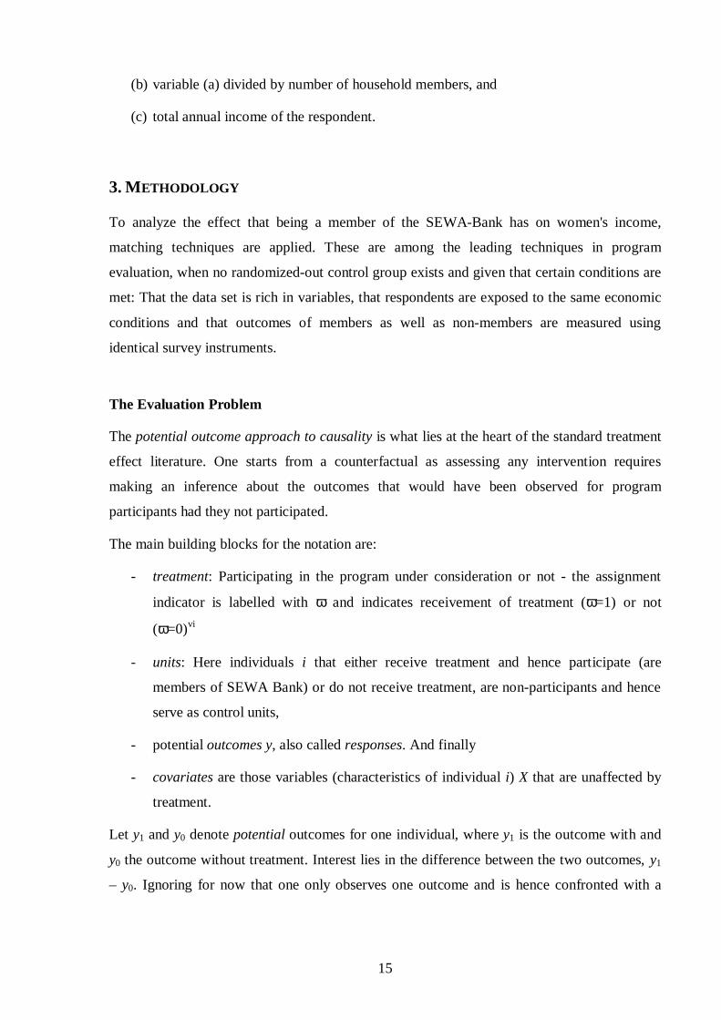
Appendix A - Probability of being a SEWA Bank member - R1

variable coef std.err P>|z|age 0.117 0.055 0.034age2 -0.001 0.001 0.039married 0.262 0.330 0.427muslim 0.488 0.239 0.041ucaste -0.855 0.242 0.000secondary school -0.256 0.266 0.335piece-rate work -0.665 0.200 0.001wage work -0.553 0.226 0.015hh head husband 0.379 0.237 0.110nuclear hh -0.475 0.233 0.041subnuclear hh -0.503 0.408 0.218highest education respondent 0.031 0.025 0.208agemax hh -0.006 0.008 0.470children 0-5 -0.078 0.106 0.464children 5-10 -0.135 0.116 0.242children 10-15 -0.069 0.122 0.571hh size -0.091 0.085 0.283house rented -0.036 0.190 0.850expenditure on food outside the house 0.048 0.018 0.009tot expenditure on food 0.005 0.004 0.225have item - other 2 -0.004 1.192 0.997have item - other 1 0.301 0.454 0.507have item - poultry 0.283 1.322 0.831have item - goat 0.192 0.451 0.670have item - sheep/goat -2.238 1.286 0.082have item - sewing machine 0.293 0.232 0.207have item - scooter 0.425 0.331 0.199have item - moped -0.165 0.183 0.367have item - bycicle 0.007 0.655 0.991have item - ivory jewelry 0.300 0.219 0.169have item - silver jewelry 0.382 0.229 0.096have item - gold jewelry 0.086 0.202 0.669have item - watches -0.053 0.161 0.744have item - clock -0.049 0.219 0.824have item - tv b&w -0.214 0.347 0.538have item - tv colour -0.179 0.193 0.355have item - tap recorder 0.161 0.220 0.465have item - radio -0.716 0.539 0.185have item - hot water hitting coil 0.334 0.247 0.177have item - mixer or blender 0.562 0.247 0.023have item - pressure cooker -0.388 0.300 0.196have item - fan 0.066 0.204 0.748have item - stove kerosene -0.293 0.346 0.397have item - utensils 0.295 0.200 0.139grade completed respondent -0.030 0.030 0.316grade enrolled 0.104 0.133 0.435enrolled yes/no -0.116 0.216 0.591amount non-sewa savings 0.000 0.000 0.082respect for contribution in hh 0.246 0.332 0.459respect for contribution in community -0.345 0.199 0.084constant -1.060 1.291 0.412Common support was chosen and yielded the following region:[0.118,0.999], percentage on common support: 98.85; Model Indications: LRChi²(50)=116.73, Pseudo R²=0.12.

34

Distribution of the estimated propensity score, R1

01

23

Den

sity

0 .2 .4 .6 .8 1Estimated propensity score

MembersNon-member

Appendix B - Probability of being a SEWA Bank member – R2

Distribution of the estimated propensity score, R2

01

23

Den

sity

0 .2 .4 .6 .8 1Estimated propensity score

MemberNon-member

35

variable coef std.err P>|z|age 0.104 0.049 0.035age2 -0.001 0.001 0.074married 0.568 0.340 0.095muslim 0.605 0.250 0.015ucaste -0.776 0.243 0.001secondary school -0.075 0.341 0.826piece-rate work -0.742 0.213 0.000wage work -0.348 0.218 0.111hh head husband 0.219 0.232 0.347nuclear hh -0.351 0.251 0.161subnuclear hh -0.043 0.456 0.925highest education respondent -0.067 0.030 0.025agemin hh 0.002 0.013 0.855agemax hh -0.019 0.009 0.030children 0-5 -0.182 0.119 0.127children 10-15 -0.266 0.112 0.018hh size 0.089 0.068 0.193house rented -0.139 0.207 0.502expenditure on food outside the house 0.017 0.012 0.144tot expenditure on food 0.004 0.004 0.336have item - other 2 0.012 0.015 0.435have item - other 1 0.002 0.021 0.905have item - poultry -0.059 0.075 0.433have item - goat 0.097 0.414 0.814have item - sewing machine 0.451 0.224 0.044have item - moped 1.033 0.589 0.079have item - bycicle 0.365 0.184 0.047have item - ivory jewelry 0.184 0.622 0.768have item - silver jewelry 0.103 0.108 0.341have item - gold jewelry -0.411 0.245 0.094have item - watches -0.137 0.204 0.501have item - clock 0.138 0.383 0.720have item - tv b&w -0.249 0.226 0.272have item - tv colour -0.059 0.289 0.838have item - tap recorder 0.065 0.189 0.730have item - radio -0.202 0.248 0.415have item - hot water hitting coil -0.569 0.483 0.239have item - mixer or blender 0.376 0.228 0.099have item - pressure cooker 0.382 0.290 0.188have item - fan 0.303 0.344 0.377have item - stove kerosene -0.311 0.355 0.381have item - utensils 0.248 0.219 0.258grade completed respondent 0.023 0.043 0.597enrolled r1 0.381 0.384 0.322enrolled r2 -0.098 0.657 0.881amount non-sewa savings 0.000 0.000 0.618respect for contribution in hh 0.160 0.420 0.703respect for contribution in community 0.448 0.224 0.045constant -2.316 1.855 0.212Common support was chosen and yielded the following region: [0.113, .987], percentage oncommon support: 99.75; Model Indications: LR Chi²(48)=111.35, Pseudo R²=0.11.

36

Appendix C - Probability of Being a First-time Borrower with the SEWA Bank

variable coef std.err P>|z|age -0.078 0.065 0.226age2 0.000 0.001 0.594married 0.913 0.957 0.340muslim -0.250 0.509 0.624ucaste -0.134 0.509 0.792secondary school 0.139 0.687 0.839piece-rate work 0.236 0.427 0.580wage work -0.148 0.480 0.758hh head husband 1.339 0.551 0.015nuclear hh 0.464 0.518 0.370subnuclear hh 1.965 1.143 0.086highest education respondent -0.076 0.067 0.252agemin hh 0.003 0.034 0.923agemax hh 0.039 0.018 0.032children 0-5 -0.376 0.262 0.152children 10-15 -0.212 0.232 0.360hh size 0.241 0.141 0.087house rented -0.639 0.483 0.186expenditure on food outside the house 0.026 0.011 0.016tot expenditure on food -0.008 0.008 0.324have item - other 2 0.000 0.032 0.991have item - other 1 -0.030 0.046 0.508have item - sewing machine 0.474 0.386 0.219have item - moped 0.546 0.767 0.477have item - bycicle -0.398 0.365 0.276have item - ivory jewelry 0.359 1.140 0.753have item - silver jewelry -0.231 0.434 0.595have item - gold jewelry 0.193 0.548 0.725have item - watches 0.281 0.445 0.527have item - clock -1.326 0.742 0.074have item - tv b&w -0.057 0.483 0.907have item - tv colour -0.044 0.583 0.940have item - tape recorder 0.255 0.372 0.493have item - radio -0.506 0.556 0.362have item - hot water hitting coil 0.426 0.841 0.612have item - mixer or blender 0.287 0.419 0.493have item - pressure cooker 1.098 0.838 0.190have item - fan 1.458 1.183 0.218have item - stove gas -0.238 0.425 0.575have item - stove kerosene -0.150 0.669 0.822have item - utensils -0.210 0.482 0.664grade completed respondent 0.015 0.090 0.871enrolled r1 1.397 1.017 0.169enrolled r2 -1.308 0.670 0.051amount non-sewa savings 0.000 0.000 0.235amount sewa savings 0.000 0.000 0.000respect for contribution in hh -0.325 0.864 0.707respect for contribution in community -0.155 0.469 0.742constant -5.488 3.104 0.077Common support was chosen and yielded the following region: [.0052, .9142] percentage oncommon support: 84; Model Indications: LR Chi²(48)=69.65, Pseudo R²=0.20.

37

Distribution of the estimated propensity score, First time borrowers

02

46

810

Den

sity

0 .1 .2 .3 .4 .5Estimated propensity score

First Time BorrowersControl

02

46

8D

ensi

ty

0 .1 .2 .3 .4 .5Estimated propensity score

First Time BorrowersControl

38

i The remaining nine objectives are to increase income security, improve nutrition and housingplus water and sanitation facilities, increase access to health services and to childcare, increasehousehold assets, self-reliance, access to education, built strong women’s organizations andwomen leaders and to improve sources of energy.ii This study works with the conventional significance level of 5%.iii For a detailed description of the methodologies used to collect data, please refer to Chen andSnodgrass (2001).iv “Rupee figures in this report are converted to dollars using appropriate market exchangerates obtained from OANDA.com and the International Monetary Fund. Rates used to deflateannual figures are averages for the last day of each month in the year. For the most relevantyears, these were 1996: 35.4 rupees to the dollar; 1997: 36.5; 1998: 41.4; and 1999: 43.2.”Chen and Snodgrass (2001)v Income figures for Round 2 were deflated to January 1998 prices by dividing by 1.156. Thiswas the value of the Ahmedabad consumer price index for labourers in January 2000,expressed on a base of January 1998. (Chen and Snodgrass, 2001, p.75)vi This is the switching regression model of Quandt (1972), the Roy model of incomedistribution (Roy, 1951; Heckman and HonorÈ, 1990) and also the Neyman-Fisher-Cox-Rubinmodel of potential outcomes.vii All results from all these analyses can be obtained from the author on request.viii This is also reflected in the sample averages in outcome variables analysed: For all differentsamples, no matter which matching technique used, the matched samples are closer in averageoutcome than the unmatched ones.ix Please note that results reported includes dummies on asset ownership. Including thesevariables assumes they cannot be influenced through attendance in the microfinance program.This might be a questionable assumption given that the program might have a strong influenceon female labour supply and hence the resources available to the household. Interpretations ofreported results do not change though, when using a propensity score without the asset-dummy variables.x As mentioned in Section 3.6 two different scenarios were estimated. Results in the table arethose where to each member corresponding/close non-members are matched. As a robustnesscheck the same estimation was repeated defining non-members as the treatment group giventhe relatively small pool of control units in the common setting. Please note though, thatreversing the setting in order to have a bigger pool of controls than treated units, does notnecessarily lead to better matches as the densities of the propensity score of the first roundshows for example that for non-members with a low propensity score, it is difficult to findclose matches.xi The corresponding propensity score specification is displayed in Appendix C.

39

REFERENCES

Aakvik, A. J.J.Heckman, E.J. Vytlacil (2005), “Estimating treatment effects fordiscrete outcomes when responses to treatment vary: An application to Norwegianvocational rehabilitation programs”. Journal of Econometrics 125 (2005), 15-51.Abadie and Imbens (2002), “Simple and bias-corrected matching estimators foraverage treatment effects, National Bureau of Economic Research, TechnicalWorking Paper 283, http://www.nber.org/papers/T0283.

Adams, D. (2001), “Crossfire”, in D. Adams and L. Mayoux (2001), Small EnterpriseDevelopment 12(1):4-6.

Agodini, R. and M. Dynarski (2004), “Are experiments the only option? A look atdropout prevention programs”, The Review of Economics and Statistics, February2004, 86(1): 180-194.Alexander, G. (2001), “An Empirical Analysis of Microfinance: Who are theClients?”, Paper presented at 2001 Northeastern Universities DevelopmentConsortium Conference.

Angrist, J.D. (2004), “Treatment Effect Heterogeneity in Theory and Practice”, TheEconomic Journal, 114 (March), C52 C83, 2004.Angrist, J.D. and J. Hahn (1999), “When to control for covariates? Panel Asymptoticsfor estimates of treatment effects.”The Review of Economics and Statistics, February2004, 86(1): 58-72.

Angrist, J.D. and A. Krueger (1990), “Does compulsory school attendanceaffectschooling and earnings?” National Bureau of economic research, Working Paper No.3572.Armendariz, B. & J. Morduch, (2003), The Economics of Microfinance, MIT Press,2005.Aroca, P. (2002), “Microcredit Impact Assessment: The Brasilian and ChileanCases”. JEL Classification: O16, O17.Bassi (1984), “The effect of CETA on the post-program earnings of participants”,Journal of Human Resources, vol. 18, pp. 539-56.Becker, S.O. & A. Ichino, “Estimation of average treatment effects based onpropensity scores. LABORatorio R. Revelli; Centre for Employment Studies.Blundell, R. & M.C. Dias (2002), “Evaluation Methods for Non-Experimental Data”.Fiscal Studies vol. 21, no. 4, pp. 427-468.Chen, S. & M. Ravallion (2003), “Hidden Impact? Ex-Post Evaluation of an Anti-Poverty Program”. World Bank Policy Research Working Paper 3049, May 2003.Chen, M.A. & D. Snodgrass (2001), “Managing resources, activities, and risk inurban India: The impact of SEWA Bank} USAID: AIMS Project, available athttp://www.usaidmicro.org/pubs/aims.

Cochran and D. Rubin (1973), “Controling Bias in Observational Studies: A Review”.Sankhya, 35, 417-46.

40

Coleman, B. (1999), “The Impact of Group Lending in Northeast Thailand.”Journalof Development Economics 60: 105-42.

Coleman, B. (2002), “Microfinance in Northeast Thailand: Who benefits and howmuch?”, Asian Development Bank, Economics and Research Department WorkingPaper No. 9, April 2002.Czarnitzki, D. & K. Hussinger (2004), “The Link Between R\&D Subsidies, R\&DSpending and Technological Performance.” Centre for European Economic Research,Discussion Paper No. 04-56.

Diaz, J.J. & S. Handa, (2004), “An Assessment of Propensity Score Matching as aNon-Experimental Impact Estimator: Evidence from a Mexican Poverty Program.”University of North Carolina.Deaton, A. (2000), “The Analysis of Household Surveys - A microeconometricApproach to Development Policy.” The International Bank for Reconstruction andDevelopment / The World Bank, Washington, D.C., USA, 2000.

Dehejia, R. (2005), “Practical propensity score matching: a reply to Smith and Todd.”Journal of Econometrics, 125 (2005), 355-36.

Dehejia,nR. & S. Whaba (2002), “Propensity score matching-methods fornonexperiimental causal studies.”The Review of Economics and Statistics, February2002, 84(1): 151-161.Fischer, T. & M.S. Sriram, (2002), Beyond Micro-Credit – Putting Development Backinto Micro-Finance, Vistaar Publications, New Delhi, 2002.Froelich, M. (2004), “Finite-sample properties of propensity-score matching andweightig estimators.” The Review of Economics and Statistics, February 2004, 86(1):77-90.

Hansen, K. & J. Heckman, K. Mullen (2004), “The effect of schooling and ability onachievement test scores.”Journal of Econometrics, 121 (2004), 39 - 98.

Hahn, J. (1998), “On the role of Propensity Score in Efficient Estimation of AverageTreatment Effects.”Econometrica 66, March 1998.

Heckman, J.J. & J. Hotz (1989), “Choosing Amount Alternative NonexperimentalMethods for Estimating the Impact of Social programs: The Case of ManpowerTraining.” JASA 84 (19989): 862-8.Heckman, J.J. & H. Ichimura, J. Smith and P. Todd (1998a), “CharacterizingSelection Bias Using Experimental Data.”Econometrica, Vol. 66, No. 5 (Sept. 1998),1017-1098.

Heckman, J.J. & H. Ichimura and P. Todd (1998b), “Matching As An EconometricEvaluation Estimator.”The Review of Economic Studies, Vol. 65, No. 2 (Apr. 1998),261-294Heckman, J.J. & H. Ichimura and P. Todd (1997), "Matching as an EconometricEvaluation Estimator: Evidence from Evaluating a Job Training Programme." Reviewof Economic Studies, October 1997, 64(4), pp. 605-54.

41

Heckman, J.J. & Vytlacil (2000) “Instrumental variables, selection models, and tightbounds on the average treatment effect.” National Bureau of Economic Research,Technical working paper 259.Hirano, K. & G.W. Imbens, G. Ridder (2003), “Efficient Estimation of AverageTreatment Effects using the Estimated Propensity Score.”Econometrica 71(4), 2003.March 1998.

Hirano, K. & G.W. Imbens (2004), ”The Propensity Score with ContinuousTreatments.” Draft Chapter of Missing Data and Bayesian Methods in Practice byDonald Rubin's Statistical Family.Imbens, G.W. (2004), “Nonparametric Estimation of Average Treatment Effectsunder Exogeneity: A Review.”The Review of Economics and Statistics, February2004, 86(1): 4-29.

Imbens, G.W. and J.D. Angrist (1994), “Identification and Estimation of LocalAverage Treatment Effects”, Econometrica, 62(2):467-75.

Jacobson, L. & R. LaLonde, D.G. Sullivan (2004), “Estimating the returns tocommunity college schooling for displaced workers.”Journal of Econometrics, 125(2005), 271-304.Johnson, M.A. & U. Akella, J. Lalande (1999), “The Impact of Outcome-BasedAssessment on Microenterprise Programs.” Journal of Microfinance, Volume 1,Number 1.

Karlan, D.S. (2001), “Microfinance Impact Assessment: The perils of using newmembers as a control group.” Journal of Microfinance, Volume 3 Number 2.

Khander, S. (2003), “Micro-finance and Poverty: Evidence Using Panel Data fromBangladesh.” World Bank Policy Research Working Paper 2945, January 2003.

Lechner, M. (1996), “The effects of enterprise-related continuous vocational trainingin East-Gemany on individual employment and earnings.” Discussion Paper \# 542-96, Beitraege zur Angewandten Wirtschaftsforschung, Universitaet Mannheim, 1996.Lechner, M. (2002), Some practical issues in the evaluation of heterogeneous labourmarket programmes by matching methods.”Royal Statistical Society 165, Part 1, pp.59-82, 2002.

McKernan, S.-M. (2002), “The Impact of Microcredit Programs on Self-employmentProfits: Do Noncredit Program Aspects Matter?” Review of Economics and Statistics84(1), February: 93-115.Michalopoulos, C. & H. Bloom, and C. Hill (2004), “Can propensity-score methodsmatch the findings from a random assignment - evaluation of mandatory welfare-to-work program?”The Review of Economics and Statistics, February 2004, 86(1): 156-179.Microcredit Summit Campaign (2000), “Empowering Women with Microcredit:Microcredit Summit Campaign Report 2000.” Countdown 2005 3 (2-3), July/August:16-31.

Morduch, J. (1998), “Does Microfinance Really Help the Poor? New Evidence onFlagship Programs in Bangladesh’, MacArthur Foundation project on inequalityworking paper, Princeton University, draft.

42

Newman, J. & M. Pradhan, L.B. Rawlings, G. Ridder, R. Coa, J.L. Evia (2002) , “AnImpact Evaluation of education, health and water supply of investments by theBolivian Social Investment Fund.” The World Bank Economic Review, Vol. 16, No.2, 241-74.

Pitt, M. & S. Khandker (1998), “The Impact of Group-Based Credit Programs onPoor Households in Bangladesh: Does the Gender of Participants Matter?” Journal ofPolitical Economy 106:5, pp. 958-996.Rosenbaum, P.R. (1987), “Model-Based Direct Adjustment.” Journal of AmericanStatistical Association, 82, 387-394.Rosenbaum, .R. (1995), Observational Studies, Springer Verlag, New York.

Rosenbaum, P.R. & D.B. Rubin (1983), “The Central Role of Propensity Score inObservational Studies for Causal Effects.” Biometrika 70[1], April 1983, 41-55

Rubin, D. (1974), “Estimating Causal Effects of Treatment in Randomized andNonrandomized Studies.” Journal of Educational Psychology, 66, 688-701.

Rubin, D. (1977), “Assignment to Treatment Group on the Basis of Covariate”,Journal of Educational Statistics, 2, 1-26.

Rubin, D. & N. Thomas (1996), “Matching using estimated propensity scores:Relating Theory to Practice”, Biometrics, 52, 249-264.

Shah, P. & N. Mandava (2005), Law, Liberty and Livelihood – Making a Living OnThe Street, Published by Academic Foundation in Association with Centre for CivilSociety, New Delhi, 2005.Subbaro, K. & K. Ezemerani, J. Randa, G. Rubio (1999), “Impact Evaluation in FY98Bank Projects: A Review.” World Bank, Poverty Reduction and EconomicManagement Network, Washington, D.C.

Smith, J.A. and P.E. Todd (2005), “Does matching overcome LaLonde's critique ofnonexperimental estimators?”Journal of Econometrics, 125 (2005), 305-353.

Smith, J.A. and P.E. Todd (2001), “Reconciling Conflicting Evidence on theperformance of PropensityScore Matching Methods”, The American EconomicReview, Vol. 91, No. 2 (May 2001), pp. 112-118.Wooldridge, J.M. (2002), Econometric Analysis of Cross Section and Panel Data.MIT Press, Cambridge, MA, 2002.Wooldridge, J.M. (2004a), “Estimating Average Partial Effects under ConditionalMoment Independence Assumptions.” working paper presented at a seminar at thePrinceton, Northwestern, Harvard/MIT, Chicago, Bristol, and the Research TriangleEconometrics Conference, 2004.Zhao, Z. (2004), Using Matching to Estimate Treatment Effects: Data Requirements,Matching Metrics, and Monte Carlo Evidence.” The Review of Economics andStatistics, February 2004, 86(1): 91-107.

43

Maastricht Graduate School of GovernanceWorking Paper Series

List of publications

2008No. Author(s) Title

001 Roelen, K. andGassmann, F.

Measuring Child Poverty and Well-Being: a literaturereview

002 Hagen-Zanker, J.Why do people migrate? A review of the theoreticalliterature

003 Arndt, C. and Omar,C.

The Politics of Governance Ratings

004 Augsburg, B. Econometric evaluation of the SEWA Bank in India:Applying matching techniques based on the propensityscore

Revised Version

2007No. Author(s) Title

001 Notten, G. and C. deNeubourg

Relative or absolute poverty in the US and EU? The battleof the rates

002 Hodges, A. A.Dufay, K. Dashdorj,K.Y. Jong, T.Mungun and U.Budragchaa

Child benefits and poverty reduction: Evidence fromMongolia’s Child Money Programme

003 Hagen-Zanker, J.and Siegel, M.

The determinants of remittances: A review of the literature

004 Notten, G. Managing risks: What Russian households do to smoothconsumption

005 Notten, G. and C. deNeubourg

Poverty in Europe and the USA: Exchanging officialmeasurement methods

006 Notten, G and C. deNeubourg

The policy relevance of absolute and relative povertyheadcounts: Whats in a number?

007 Hagen-Zanker, J.and M. Siegel

A critical discussion of the motivation to remit in Albaniaand Moldova

008 Wu, Treena Types of Households most vulnerable to physical andeconomic threats: Case studies in Aceh after the Tsunami

009 Siegel, M. Immigrant Integration and Remittance Channel Choice

2006No. Author(s) Title

001 Gassmann, F. andG. Notten

Size matters: Poverty reduction effects of means-tested anduniversal child benefits in Russia

002 Hagen-Zanker, J.andM.R. Muñiz Castillo

Exploring multi-dimensional wellbeing and remittances inEl Salvador

003 Augsburg, B. Econometric evaluation of the SEWA Bank in India:Applying matching techniques based on the propensityscore

44

(See 2008WP004 for revised version)

004 Notten, G. andD. de Crombrugghe

Poverty and consumption smoothing in Russia

2005No. Author(s) Title

001 Gassmann, F. An Evaluation of the Welfare Impacts of ElectricityTariff Reforms And Alternative CompensatingMechanisms In Tajikistan

002 Gassmann, F. How to Improve Access to Social Protection for the Poor?Lessons from the Social Assistance Reform in Latvia