Econometric analysis of quantile regression models and ...
105
Inauguraldissertation zur Erlangung des akademischen Grades eines Doktors der Wirtschaftswissenschaften Der Universit¨ at Mannheim Econometric analysis of quantile regression models and networks With empirical applications Maria Marchenko Juni 2016
Transcript of Econometric analysis of quantile regression models and ...
Inauguraldissertation zur Erlangung desakademischen Grades eines Doktors der
Wirtschaftswissenschaften Der Universitat Mannheim
Econometric analysis of quantile regression models
and networks
With empirical applications
Maria Marchenko
Juni 2016

Abteilungssprecher: Prof. Dr. Carsten Trenkler
Referent: Prof. Dr. Enno Mammen
Koreferent: Prof. Dr. Markus Frolich
Datum des mundlichen Prufung: 19.Juli 2016
ii

Eidesstattliche Erklarung
Hiermit erklare ich, dass ich die vorliegende Dissertation selbstandig angefertigt und die be-
nutzten Hilfsmittel vollstandig und deutlich angegeben habe.
Maria Marchenko 16. Juni 2016
iii

iv

Acknowledgements
First and foremost, I would like to express my gratitude to my advisor Enno Mammen forhis massive support and help, and his boundless patience. I have benefited and learned a lotfrom our joint work. It was a terrific and fruitful experience, which also resulted in the firstchapter of this thesis.
I am very thankful to Markus Frolich for finding the time to be a co-referent of thisthesis.
I am deeply grateful to Andrea Weber for her tremendous support and invaluablecomments on the second chapter of this thesis.
My sincere thanks go to Maria Yudkevich for giving me the chance to work withthe network data from Higher School of Economics and to the team of Center of Institu-tional Studies of HSE. The financial support from the Government of the Russian Federationwithin the framework of the Basic Research Program at the National Research UniversityHigher School of Economics and within the framework of the implementation of the 5-100Programme Roadmap of the National Research University Higher School of Economics isacknowledged.
I also want to thank my brother-in-law, Sergey Merzlikin, for sharing his computerskills, without which I most likely wouldn’t have been able to get the data for the thirdchapter.
I had the opportunity to present the individual chapters of this thesis at variousseminars, conferences, and workshops, and I appreciate numerous comments and sugges-tions received from the participants at these events. I am grateful for fruitful discussionsand helpful comments from Andreas Dzemski, Jan Nimczik, Anna Hammerschmid, MariaIsabel Santana, Florian Sarnetzki, Stephen Kastoryano, Petyo Bonev, Jasper Haller. I wantto thank the CDSE (Center for Doctoral Studies in Economics) for the great program andfinancial support, and all my CDSE colleagues, many of which have become my dear friends,for the unforgivable time in Mannheim.
And last but not the least, I am indebted to my parents for their continuous andunconditional support, my grandmother and late great-grandmother for their prayers, mysister Oksana for being my best friend and not letting me give up and my nephew Semionfor being the most loving and lovable kid in the world.
v

vi

Contents
Introduction 1
Chapter 1 . . . . . . . . . . . . . . . . . . . . . . . . . . . . . . . . . . . . . . . . . 1
Chapter 2 . . . . . . . . . . . . . . . . . . . . . . . . . . . . . . . . . . . . . . . . . 2
Chapter 3 . . . . . . . . . . . . . . . . . . . . . . . . . . . . . . . . . . . . . . . . . 3
1 Weighted average estimation in nonparametric higher-dimensional quan-tile regression: joint with Enno Mammen 5
1.1 Introduction . . . . . . . . . . . . . . . . . . . . . . . . . . . . . . . . . . . . . 5
1.2 Problem formulation and theory . . . . . . . . . . . . . . . . . . . . . . . . . 7
1.3 Proof of Theorem 1.1 . . . . . . . . . . . . . . . . . . . . . . . . . . . . . . . . 10
References, chapter 1 . . . . . . . . . . . . . . . . . . . . . . . . . . . . . . . . . . . 17
2 Endogenous Shocks in Social Networks: Effects of Students’ Exam Retakeson their Friends’ Future Performance 18
2.1 Introduction . . . . . . . . . . . . . . . . . . . . . . . . . . . . . . . . . . . . . 18
2.2 Model . . . . . . . . . . . . . . . . . . . . . . . . . . . . . . . . . . . . . . . . 21
2.2.1 Naıve approach . . . . . . . . . . . . . . . . . . . . . . . . . . . . . . . 21
2.2.2 Proposed model with no correlated effects . . . . . . . . . . . . . . . . 24
2.2.3 Model with correlated effects . . . . . . . . . . . . . . . . . . . . . . . 26
2.2.4 Estimation strategy . . . . . . . . . . . . . . . . . . . . . . . . . . . . 27
2.3 Data and Descriptive analysis . . . . . . . . . . . . . . . . . . . . . . . . . . . 31
2.3.1 The system of higher education in Russia and specifics of the sampleduniversity. . . . . . . . . . . . . . . . . . . . . . . . . . . . . . . . . . . 31
2.3.2 Data description . . . . . . . . . . . . . . . . . . . . . . . . . . . . . . 32
2.3.3 Network characteristics . . . . . . . . . . . . . . . . . . . . . . . . . . 35
vii

2.3.4 Descriptive analysis . . . . . . . . . . . . . . . . . . . . . . . . . . . . 37
2.4 Results . . . . . . . . . . . . . . . . . . . . . . . . . . . . . . . . . . . . . . . . 39
2.4.1 Main specification . . . . . . . . . . . . . . . . . . . . . . . . . . . . . 39
2.4.2 Connection to one’s own retake . . . . . . . . . . . . . . . . . . . . . . 41
2.4.3 Effects in different departments . . . . . . . . . . . . . . . . . . . . . . 43
2.4.4 Estimation in presence of correlated effects . . . . . . . . . . . . . . . 44
2.4.5 Additional analysis . . . . . . . . . . . . . . . . . . . . . . . . . . . . . 45
2.5 Conclusion . . . . . . . . . . . . . . . . . . . . . . . . . . . . . . . . . . . . . 47
Appendix . . . . . . . . . . . . . . . . . . . . . . . . . . . . . . . . . . . . . . . . . 49
Appendix A. Main proofs . . . . . . . . . . . . . . . . . . . . . . . . . . . . . 49
Appendix B. Additional tables and figures . . . . . . . . . . . . . . . . . . . . 57
References, chapter 2 . . . . . . . . . . . . . . . . . . . . . . . . . . . . . . . . . . . 64
3 Peer effects in art prices 65
3.1 Introduction . . . . . . . . . . . . . . . . . . . . . . . . . . . . . . . . . . . . . 65
3.2 Model . . . . . . . . . . . . . . . . . . . . . . . . . . . . . . . . . . . . . . . . 66
3.2.1 Hausman and Taylor type models . . . . . . . . . . . . . . . . . . . . 68
3.2.2 Alternative approach . . . . . . . . . . . . . . . . . . . . . . . . . . . . 69
3.3 Data description . . . . . . . . . . . . . . . . . . . . . . . . . . . . . . . . . . 70
3.4 Empirical analysis . . . . . . . . . . . . . . . . . . . . . . . . . . . . . . . . . 75
3.4.1 Subsample of sold lots . . . . . . . . . . . . . . . . . . . . . . . . . . . 75
3.4.2 Full sample . . . . . . . . . . . . . . . . . . . . . . . . . . . . . . . . . 78
3.4.3 Full sample, Maximal and Minimal Estimated Prices . . . . . . . . . . 80
3.5 Conclusion . . . . . . . . . . . . . . . . . . . . . . . . . . . . . . . . . . . . . 82
Appendix C. Additional figures . . . . . . . . . . . . . . . . . . . . . . . . . . . . . 84
References, chapter 3 . . . . . . . . . . . . . . . . . . . . . . . . . . . . . . . . . . . 92
Full Bibliography 93
viii
Introduction
This thesis consists of three essays that address open research issues in two econo-metric frameworks: nonparametric quantile regression framework and social networks, sup-ported by empirical applications. Both econometric approaches are used to achieve a deeperunderstanding of the economic processes and interactions in comparison to the simple meanregression.
Quantile regression, discussed in Chapter 1, allows estimating and analysing thewhole conditional distribution and, therefore, is able to differentiate the effect for the differ-ent quantiles of the outcomes. Quantile regression has various applications and is especiallypopular in socio-economic problems, analysis of individual and household finances, demandelasticities and many others. In most of this cases, more than one covariates are expected tobe included in the model. However, once the nonparametric approach is chosen, the so-calledcurse of dimensionality arises. With the optimal choice of bandwidth h, the dimension ofthe covariate vector under which the inference and testing are possible might be insufficientfor the empirical analysis. Chapter 1 proposed a possible improvement of the nonparametricquantile regression estimation.
Chapters 2 and 3 explore the research questions in the network analysis. Linkedagents are likely to have exhibit similar behaviour, hence, the inclusion of the network infor-mation into the analysis improves the understanding of the outcome determinants. Identifi-cation of the network effects is usually quite complex due to the reflection problem introducedby Manski (1993): the outcomes of the connections that influence one’s own outcomes are af-fected in its turn by the outcomes. Once the network is known, the identification is achievedfor the most types of the networks, under assumptions shown in Bramoulle, Djebbari, andFortin (2009). However, modifications of the classical model may require further thoroughanalysis. Dynamic network model with endogenous shock (Chapter 2 ) and panel data modelwith fixed network (Chapter 3 ) are the examples of such modifications, required by the spe-cific empirical examples.
Chapter 1
In the first chapter (based on joint work with Enno Mammen), I consider a problemof studying the asymptotic properties of the quantile regression estimation under increasingdimensions in the nonparametric setting. A classical approach for the analysis of the para-metric and nonparametric quantile estimators use Bahadur expansion, which distinguishestwo parts of conditional quantile model: the mean regression and the remainder. However,Bahadur expansion requires too restrictive assumptions for the asymptotic analysis. In alot of interesting cases, the remainder part of the Bahadur expansion has a slower rate ofconvergence than the main part, and the asymptotic inference and testing is not valid forthe models with more than one covariate.
1

2 Introduction
In this chapter, asymptotic properties of marginal averages of kernel quantile estima-tors are discussed. This estimator arises in some treatment settings, as well as in single-indexand partially-linear models and it can be further applied for testing procedures. Asymptoticexpansions are developed for higher order terms that allow analysing under which conditionson the dimension of the covariates and on the smoothness of the underlying densities theestimator is consistent. The mathematical approach makes use of higher order Edgeworthexpansions that allow calculating moments of the nonparametric kernel quantile estimator.
It was possible to show that the considered weighted average estimator works andachieves
√n rates with a normal limit for the dimensions d = 2 and d = 3 under a cer-
tain assumption, but the generalization for all functional forms of the model and for higherdimensions will not work. The first chapter provides the thorough proof of this result.
Chapter 2
In the second chapter, I discuss the dynamic behaviour of connected agents in re-sponse to the endogenous shock. I pursue the idea, that the shocks or the treatment hap-pening to one of the players in the network influence not only their future performance butalso affect all their network connections. This idea is closely related to the logic behindthe spillovers in different settings, in particular, knowledge spillovers via conversational net-works. I combine it with the logic used in peer effect literature to develop the dynamic modelof network behaviour. Unlike spillovers, the shock on the network considered in this chapteranalysis only influence the first-level connections.
Standard peer effect approach explores the co-movement, simultaneous outcomesof connected agents. Manski (1993) distinguishes three effects that determine the similarbehaviour of peers. The endogenous effect suggests that the performance of an agent will beaffected by the average performance of the peer group or network connections. The exogenouseffect uses mean exogenous characteristics of the peer group to determine the performance.The correlated effect appears due to the similar individual characteristics within a group.The most important task of peer effects analysis is to determine the endogenous effect, whichcan have important policy implications. Some of the examples of the peer effect analysisare Ammermueller and Pischke (2009), who discusses the achievements of the peers in theprimary schools, Bruce Sacerdote (2001) and Androushchak, Poldin, and Yudkevich (2013),who look at the exogenously formed groups to study the peer effects in the college or uni-versity, Gaviria and Raphael (2001), who study the influence of peers on juvenile behaviour,and many others in various empirical frameworks. The studied outcomes of peers are of thesame period. However, the significant individual event is likely to have an importance forthe one’s connections. Comola and Prina (2014) is the closest to discuss such a networkdynamics. They are using the randomized treatment as a shocking event, which is clearlyexogenous in the model, although it is not necessarily the case in a more general setting. Forexample, shocks in educational frameworks, such as exam failures or dropouts are to a bigextent determined by the network itself, and hence are endogenous.
This chapter develops the dynamic peer effect model with a shock, accounting forits possible endogeneity as well as for the changes happening to the network as a responseto the shock. The model allows to predict the endogenous part of the shock and use theunexpected component to estimate the effect of pure shock. Due to simultaneous influenceof connected elements on each other, a model with social interactions alone requires a partic-ular exogenous variation to identify the endogenous effect. The inclusion of the endogenousshock in the model make identification more complex. In this chapter, I derive and prove theidentification conditions for both the endogenous effect and the effect of the shock for the
3
network case, which require variability of the network as well as the existence of intransitivetriads for the model without correlated effects or the distances of length three for the modelwith correlated effects. Intransitive triads appear when some two nodes of the network arenot connected directly, but via the third node, the distances of length three require theexistence of two nodes, the shortest distance between which is three links, i.e. there aretwo nodes between them. The latter identifying assumptions were proposed in Bramoulle,Djebbari, and Fortin (2009), whereas the former assumption is novel for the literature.
I also propose the estimation procedure that uses the exogenous characteristics ofthe first or the second level of connections, depending on the type of model, as instrumentalvariables and yields the consistent estimation.
The empirical part of this chapter makes the contribution to the strain of literatureanalysing peer effects in educational settings. I use the dynamic network data of univer-sity students to test the model. I treat exam retakes as endogenous shocks and estimatethe effect of the unexpected component of friends’ retakes on one’s own average grade. Itis suggested that the unexpected shock, especially in the important subjects, may have acertain psychological influence on the connections. I apply the estimation procedure to thedata on the students in HSE, Nizhniy Novgorod. The results indeed suggest that on averagethe retake of the friend may have an effect on future performance, and this effect appears tobe negative, however, it has a different magnitude for students of different departments, aswell as for students with and without own retake.
Chapter 3
In the third chapter, I continue analysing the network environment. I apply the
standard peer effect ideology to a rather unusual setting. I assume that the connections in
the art world may have an influence on both the development of the art skills and talent and
reputation of a particular artist. Art market always attracted a lot of money and attention
and is booming in the recent years. Quoting seminal paper by Baumol (1986), ”prices [of
art objects] can float more or less aimlessly and their unpredictable oscillations are apt to
be the exacerbated by the activities of those who treat such art objects as ”investments”.
He suggests that buying art is not likely to deliver any real rate of return different from
zero. However, the big strain of the literature come up with a different conclusion either by
improving the method or the data used for the analysis. For example, Goetzmann (1993)
reports an average annual real return on oil paintings of 3.8% for the period between 1850
and 1986, with returns around 15% after 1940, Mei and Moses (2002) - the return of 4.9% for
1875-1999, with 8.2% after 1950, Renneboog and Spaenjers (2013) - 3.97% over the period
1957-2007.
Among businessmen and collectors, art is indeed often considered as an attractive
investment, being one of the possible so-called passion good. Therefore, understanding the
price formation is crucial for the potential buyers. As noticed in Baumol (1986), art prices
are very unpredictable. Of course, the obvious factors influencing the price are the type of a
work, its style, the supply of other works by the same artist, his or her level of recognition
and popularity. But sometimes, especially within one particular style, these factors are not
enough, and the prices achieve unexpected values. In this chapter, I explore one of the deter-

4 Introduction
minants of art price formation, not included into the analysis in previous literature: artists’
connections. Connections are suggested to matter due to the already discussed logic of the
peer effect analysis as well as by affecting the reputation of particular artists. The more
valuable the works of artists’ connection, the more likely the connections are to be popular
and well-known not only in the art circles. Connecting to more popular artists may result in
better reputation. I believe that the potential buyers will react differently, when they learn
that the artist was a friend of Pablo Picasso and when they are told that the artist worked
together with, for example, Morgan Russel, who was also an important figure in an abstract
movement, but who are far less known than Picasso. Abstract art is in general harder to
evaluate, since the quality of the work and techniques is not so straightforward, especially for
a non-specialist. The network diagram prepared for the ”Inventing abstraction” exhibition
in MOMA, New York gave an idea to explore the networks further in the art prices setting.
I combine the information about the connections of the artists of the abstract move-
ment with the auction prices of their work and apply the peer effect model to estimate the
possible effect of the average price of artists connections on the price of artists’ own work.
The collected data has a panel structure, however, the network is considered constant. The
discussed auctions cover the period of 2000-first half of 2015, whereas the connections were
formed in the beginning of the 20th century, mainly in 1910-1925, so the connections are
well-known during the auction period. The fixed network makes the usage of the fixed effects
model with instrumental variables as discussed in Bramoulle, Djebbari, and Fortin (2009)
impossible since the invariant covariates are not identifiable. I propose the adaptation of
Hausman and Taylor (1981) approach with additional instrumental variables for the endoge-
nous effect of Bramoulle, Djebbari, and Fortin (2009) type. Combining these two methods
allows identifying coefficients for both variant and fixed covariates, including the endogenous
effect.
The results of the analysis suggest the presence of endogenous peer effect, however,
its direction differs for the final prices achieved on the market and prices expected by the auc-
tioneer. The auctioneer is likely to consider connected as substitutes, alternatively the higher
the value of connections’ works, the more likely the artist to be ”worse” than his peers. The
market, however, exhibits similar demand behaviour towards the connected artists leading
to the increase in one’s own price as the connections’ works become more valuable.
Chapter 1
Weighted average estimation in
nonparametric higher-dimensional
quantile regression
joint with Enno Mammen
1.1 Introduction
For a dataset of n i.i.d. tuples (Xi, Yi) we consider a nonparametric quantile regres-
sion model:
Yi = qα(Xi) + εi,α (i = 1, . . . , n). (1.1)
Here, Yi is a one-dimensional response variable and Xi is a d-dimensional covariate. The
function mα(Xi) is the conditional α-quantile of Yi given Xi = x for 0 < α < 1. Thus, the
conditional α-quantile of the error variables εi,α, given Xi is equal to 0. From now on, we
fix the value of α and we write also q and εi instead of qα and εi,α. We are interested in the
estimation of a weighted average θ of q:
θ =
∫q(x)ω(x)dx (1.2)
for a weight function ω. We discuss the following plug-in estimator
θ =
∫q(x)ω(x)dx (1.3)
where a kernel quantile estimator q is plugged into (1.2).
The value of θ can be of direct interest in a statistical analysis. It also arises naturally
in single index quantile models where q(x) = g(xᵀβ) for some unknown function g : R→ Rand unknown parameter β ∈ Rd. For a differentiable function w : Rd → R with compact
5
6 Chapter 1. Weighted average estimation in higher-dimensional QR
support one gets that with γ =∫g′(xᵀβ)w(x)dx
γβ =
∫q′(x)w(x)dx = −
∫q(x)w′(x)dx.
Thus,∫q(x)w′(x)dx is equal to a multiple of β. Thus, the estimation of β can be
reduced to estimation of θ with ω equal to the components of w′(x). This approach has also
been called average derivative estimation and was developed in Hardle and Stoker (1989) for
mean regression and adapted to quantile regression in Chaudhuri, Doksum, and Samarov
(1997).
A classical mathematical approach for the understanding of parametric and non-
parametric quantile estimators makes use of Bahadur expansions which transform condi-
tional quantile models to mean regression, see e.g. Chaudhuri (1991) for a discussion of
locally polynomial estimators and He and Ng (1999) and He, Ng, and Portnoy (1998) for
splines. Other references are El Ghouch and Van Keilegom (2009), Hong (2003), Hoderlein
and Mammen (2009), Kong, Linton, and Xia (2010), Y. K. Lee and E. R. Lee (2008), Li
and Racine (2008), Koenker, Ng, and Portnoy (1994), Portnoy (1997), Dette and Volgushev
(2008), Belloni, Chernozhukov, and Fernandez-Val (2011) and others.
It was observed in Mammen, Van Keilegom, and Yu (2015) that the use of Ba-
hadur expansions for the asymptotic analysis of a goodness-of-fit test in nonparametric
quantile regression may require too restrictive assumptions, which will not allow developing
the asymptotics of the estimator in some interesting cases. In their setting direct application
of Bahadur expansion would need the bandwidth h of a kernel regression quantile estimator
to fulfill the condition nh3d → ∞ for n → ∞. If the bandwidth is chosen as rate optimal,
e.g. h ∼ n−1/(4+d) for the estimation of twice differentiable functions, the assumption will
only allow one-dimensional covariates. Then, this approach allows no inference and testing
results for multidimensional models, d > 1.
In this paper we will show an expansion for the estimator q, see (1.3). In the deriva-
tion of the expansion we will make use of the fact that the kernel quantile estimator and
its Bahadur expansion are asymptotically independent if they are calculated at points that
differ more than a constant times the bandwidth h. Similarly as in Mammen, Van Keilegom,
and Yu (2015), we will use Edgeworth expansions for a statistic in a dual problem to get
expansions of moments of the kernel quantile estimator and its Bahadur representation.
The paper is organized as follows. In the next section, we will discuss the model,
state our main result on the asymptotics of the proposed estimator along with possible
applications. Section 3 gives the proof of the main result.
1.2. Problem formulation and theory 7
1.2 Problem formulation and theory
We are interested in studying the estimation by the estimator (1.3) in model (1.1).
We will use the kernel quantile estimator that is defined by:
q(x) = argminκ
n∑i=1
K
(x−Xi
h
)τ(Yi − κ), (1.4)
where K(u1, . . . , ud) = Πdj=1k(uj) with a one-dimensional symmetric kernels k and where
τ = τα is the check function τα(u) = αu+−(1−α)u− with u+ = uI(u > 0) and u− = uI(u <
0). We assume that the bandwidths h1, . . . , hd are of the same order, and for simplicity, that
they are also identical. We write h = h1 = · · · = hd. The theoretical discussions in this paper
are restricted to the case that k are positive functions. Thus k is a Nadaraya-Watson like
estimator with kernel of order one. We will comment on Nadaraya-Watson smoothing with
higher order kernels and on local polynomial smoothing below but we will state no results
for these smoothing methods. An essential argument in our proof cannot be extended to
this case. For the following discussion we will assume that q has two derivatives.
Following Chaudhuri (1991), see also Theorem 2 in Guerre and Sabbah (2012), the
Bahadur approximation of q is given by:
q(x)− q(x) =
∑ni=1K
(x−Xih
){I(Yi − q(Xi) ≤ 0)− α}∑n
i=1K(x−Xih
)fε|X(0|Xi)
+OP (Ln(nhd)−3/4), (1.5)
where fε|X is the conditional density of εi, given Xi. Here and in the following, we write
Ln for sequences that fulfill Ln = O((log n)C) for a constant C > 0 large enough. This
expansion holds uniformly over compact subsets of Rd. Thus, if ω has a compact support
we get that
θ − θ =
∫ ∑ni=1K
(x−Xih
){I(Yi − q(Xi) ≤ 0)− α}∑n
i=1K(x−Xih
)fε|X(0|Xi)
ω(x)dx+OP (Ln(nhd)−3/4). (1.6)
We now discuss if this expansion can be used to show that√n(θ − θ) has an asymptotic
mean zero normal limiting distribution. The mean of the first term on the right hand side of
(1.6) is of order h2. This follows by standard smoothing theory using our assumption that q
has two derivatives. Thus if we want to prove that√n(θ − θ) has an asymptotic mean zero
normal limiting distribution, expansion (1.6) can only be used if h2 + (nhd)−3/4 = o(n−1/2).
Such choices of h only exist for d = 1.
The aim of this paper is to study if the estimator θ still works for d > 1 and achieves√n rates with a normal limit, for an appropriate choice of the bandwidth h. We will show
that this is not the case and that the estimator for all choices of h does not has a√n rate. The
next question is if for d > 1 it is possible to construct an estimator of θ with√n-consistency
and normal limit that works if we only make the assumption that q has two derivatives. We
8 Chapter 1. Weighted average estimation in higher-dimensional QR
will give a positive answer to this question for d = 2 and d = 3. Our estimator of θ is based
on the calculation of q for several bandwidths h.
For our theory, we need to make the following assumptions. We use the convention
that C is a generic strictly positive constant chosen large enough and that c is a generic
strictly positive constant chosen small enough. As above, we also write Ln = (log n)C for a
sequence with C > 0 large enough.
(A1) The support RX of X is a compact convex subset of Rd. The density fX of X is
strictly positive and continuously differentiable on the interior of RX . The conditional
density fε|X(e|x) is uniformly bounded over x, e.
(A2) The cumulative distribution function FY |X(·|x) of the conditional distribution of Y
given X = x is twice continuously differentiable with respect to x and has a continu-
ously differentiable density fY |X(·|x) that satisfies
fY |X(y|x) > 0,
|fY |X(y′|x′)− fY |X(y|x)| ≤ C(||x′ − x||+ |y′ − y|)
for x, x′ ∈ RX and y, y′ ∈ R, where || · || is the Euclidean norm. The density fε|X(ε|x)
and its derivative with respect to ε is twice differentiable in x for ε in a neighborhood
of 0.
(A3) The kernel k is a symmetric, continuously differentiable probability density function
with compact support (w.l.o.g, equal to [−1, 1]). It fulfills a Lipschitz condition and it is
monotone strictly increasing on [−1, 0]. It holds that k′(k−1(u)) ≥ min c{uκ, (k(0)−u)κ
for some κ > 0 where k−1: [0, k(0)] → [−1, 0] denotes the inverse of k: [−1, 0] →[0, k(0)]. The bandwidth h satisfies h = o(1) and nhd/Ln →∞.
(A4) The function ω(x) is Lipschitz-continuous: |ω(x′−ω(x)| ≤ C||x′−x|| for all x, x′ ∈ RX .
Now we can state our main result.
Theorem 1.1 Assume (A1)-(A4). Then,
θ − θ =
∫q(x)ω(x)dx+ h2
∫q′′0(x) + 1
2q′0(x)f ′X
fε|X(0|x)fX(x)ω(x)dx+ o(h2)
+1
nhd
∫ [fε|X(0|x)fX(x)
∫K2(u)du+
1
2
∂εfε|X(0|x)
fε|X(0|x)ω(x)
]dx
+O(Ln(nhd)−3/2
)+OP (Lnn
−3/4h−d/4)
where we put
q(x) =
∑ni=1K
(x−Xih
){I(Yi − qh(x) ≤ 0)− α}∑n
i=1K(x−Xih
)fε|X(0|Xi)

1.2. Problem formulation and theory 9
with qh(x) such that
E[K
(x−Xi
h
){I(Yi − qh(x) ≤ 0)− α}
]= 0.
Furthermore, it holds that√n
∫q(x)ω(x)dx
d→ N (0, V ),
where
V = α(1− α)
∫ω2(x)
fX(x)f2ε|X(0|x)dx.
We now discuss applications of this result. First we will discuss if there exist estimates
of θ that are based on q and that achieve a parametric√n-rate of convergence. For
√n-
consistency we need that the bias of q is of order o(n−1/2). This requires that h = o(n−1/4).
Under this assumption the estimator q is not consistent if d ≥ 4. Thus√n-consistent esti-
mation of θ based on q is not possible for d ≥ 4. For d = 1 we can choose the bandwidth
h such that h = o(n−1/4), Ln(nhd)−1 = o(n−1/2) and Lnn−3/4h−d/4 = o(n−1/2). For such a
choice of h we get that θ − θ =∫q(x)ω(x)dx + oP (n−1/2). Thus we have a
√n-consistent
estimator of θ with asymptotic normal limit.
For d = 2 there exists no choice of the bandwidth h such that h = o(n−1/4),
Ln(nhd)−1 = o(n−1/2) and Lnn−3/4h−d/4 = o(n−1/2). Thus we need here another approach.
We propose to calculate θ for three choices of bandwidths, h1, h2 and h3, say, which fulfill
hj = o(n−1/4), Ln(nhdj )−3/2 = o(n−1/2) and Lnn
−3/4h−d/4j = o(n−1/2) for j = 1, .., 3. This
gives three values θ1, θ2 and θ3 for which it holds that
θj = an,0 + an,1h2j + an,2
1
nhd+ oP (n−1/2)
for j ∈ {1, 2, 3} where an,0 = θ +∫q(x)ω(x)dx. The three values θ1, θ2 and θ3 can be used
to get least squares fits an,0, an,1 and an,2 of an,0, an,1 and an,2. It holds that an,0 − an,0 =
oP (n−1/2), h2j (an,1 − an,1) = oP (n−1/2) and (nhd)−1(an,2 − an,2) = oP (n−1/2). We choose
θ = an,0 as our estimator of θ. By construction we have that θ−θ =∫q(x)ω(x)dx+oP (n−1/2).
Thus, we have a√n-consistent estimator of θ with asymptotic normal limit.
For d = 3 we need a stronger result than Theorem 1.1. Under slightly stronger
smoothness conditions on the conditional density fε|X one can show the following higher
order expansion:
θ − θ = an,0 + an,1h2 + an,2
1
nhd+ an,3
1
(nhd)3/2o(h2) +O
(Ln(nhd)−2
)+OP (Lnn
−3/4h−d/4)
with an,0 =∫q(x)ω(x)dx and appropriate choices of an,1,..., an,3. This can be shown by
the same arguments as used in Theorem 1.1 but with a higher order Edgeworth expansion.
Now one chooses four bandwidths h1, ..., h4 with hj = o(n−1/4), Ln(nhdj )−2 = o(n−1/2) and
Lnn−3/4h
−d/4j = o(n−1/2) for j = 1, .., 4. This gives four values θ1, ..., θ4 that can be used
to fit an,0,..., an,3. Again, we propose θ = an,0 as our estimator of θ. By construction we
10 Chapter 1. Weighted average estimation in higher-dimensional QR
have again that θ − θ =∫q(x)ω(x)dx+ oP (n−1/2) and thus, we have again a
√n-consistent
estimator of θ with asymptotic normal limit.
We conjecture that similiar expansions as in Theorem 1.1 are valid for kernel quantile
estimators with higher order kernels and for local polynomial estimators of q. In such
expansions it is expected that the bias term of order h2 and error bound o(h2) is replaced
by a term of order h2k and error bound o(h2k) with an appropriate choice of the order
k. Unfortunately, one of our main arguments in the proof cannot be extended to these
estimators.
1.3 Proof of Theorem 1.1
For the proof we need some additional notation.
We put
q∗(x) =
q(x), if |q(x)− qh(x)| ≤ Ln(nhd)−1/2
q(x), otherwise.
For the proof we also have to define local neighborhoods. For this definition suppose first
that X is one-dimensional. Then the support RX is a compact interval. For arbitrary j and
for k ∈ {1, 2, 3}, we can then define
Ijk = [(3j + k − 1)h, (3j + k)h], and I∗jk = [(3j + k − 2)h, (3j + k + 1)h].
The set of indices of the Xi (i = 1, . . . , n) that fall inside the interval I∗jk is denoted by Njk.We write Njk for the number of elements of Njk. An arbitrary x ∈ RX belongs to a unique
Ijk and we define N (x) = Njk and N(x) = Njk. If the dimension of X is larger than one,
this partition of the support into small intervals can be generalized in an obvious way.
We also put N−(x) = {u : xj − h ≤ uj ≤ xj + h for all j = 1, . . . , d}. This is the
support of the kernel h−dK(h−1[x−·]). We also write N−(x) for the random number of Xi’s
that lie in N−(x). Note that N−(x) ⊂ N (x) and N−(x) ≤ N(x). We use the shorthand
notation m0 = nhd.
For the proof of Theorem 1.1, it is useful to consider the following decomposition:
θ − θ =
∫(q(x)− q(x))ω(x)dx (1.7)
=
∫[q(x)− q∗(x)]ω(x)dx
+
∫[E{q∗(x)− q(x)− qh(x)|N(x)}]ω(x)dx
+
∫[{q∗(x)− E[q∗(x)|N(x)]} − {q(x)− E[q(x)|N(x)]}]ω(x)dx
+
∫[q(x)− q(x)]ω(x)dx
+
∫qh(x)ω(x)dx
= θn1 + ...+ θn5.
1.3. Proof of Theorem 1.1 11
For the discussion of the terms θn1, ..., θn5 we need the following lemmas.
The following lemma gives a bound on the Bahadur expansion for q. It can be shown
by a small modification of the proof of Theorem 2 in Guerre and Sabbah (2012).
Lemma 1.1 Suppose that the assumptions of Theorem 1.1 are satisfied. Then,
supx∈Rx
|q(x)− q(x)− qh(x)| = Op((nhd)(−3/4)Ln).
The following two lemmas follow by standard smoothing theory.
Lemma 1.2 Suppose that the assumptions of Theorem 1.1 are satisfied. Then,
supx∈Rx
|q(x)| = Op((nhd)(−1/2)Ln).
Lemma 1.3 Suppose that the assumptions of Theorem 1.1 are satisfied. Then,
supx∈Rx
∣∣∣∣∣qh(x)− h2q′′0(x) + 1
2q′0(x)f ′X
fε|X(0|x)fX(x)
∣∣∣∣∣ = o(h2).
From Lemmas 1.1–1.3 we get that q(x) = q∗(x) for all x ∈ Rx with probability
tending to one. This gives
θn1 = oP (an) (1.8)
for any sequence {an} of positive constants tending to zero as n → ∞. Furthermore, from
Lemma 1.3 we get that
θn5 = h2∫q′′0(x) + 1
2q′0(x)f ′X
fε|X(0|x)fX(x)ω(x)dx+ o(h2). (1.9)
We now consider the third summand θn3.
Lemma 1.4 Suppose that the assumptions of Theorem 1.1 are satisfied. Then,
θn3 = OP (Lnn−3/4h−d/4). (1.10)
Proof of Lemma 1.4. For simplicity we consider first the one-dimensional case. The term
θn3 can be splitted into three summands (for k = 1, 2, 3):
θn3,k =∑j
∫Ijk
[{m∗(x)− E[m∗(x)|N(x)]} − {m(x)− E[m(x)|N(x)]}]ω(x)dx.
The terms θn3,1, θn3,2 and θn3,3 are sums of O(h−1) conditionally independent sum-
mands. The summands are uniformly bounded by a term of order OP (Lnn−3/4h−1/4). This
12 Chapter 1. Weighted average estimation in higher-dimensional QR
follows from Lemma 1.1 and from the fact that q(x) = q∗(x) for all x ∈ Rx with proba-
bility tending to one. Thus for k ∈ {1, 2, 3} the second conditional moment of θn3,k is of
order OP (Lnn−3/2h−1/2). This shows that θn3,k = OP (Lnn
−3/4h−1/4) for d = 1 and for
k ∈ {1, 2, 3}, which implies the statement of the lemma for d = 1. For d > 1 one can use the
same approach.
Lemma 1.5 Suppose that the assumptions of Theorem 1.1 are satisfied. Then,
E{q∗(x)− qh(x)
∣∣∣N(x)}
= m−10
2κ1,1(h, x)(κ2,1(h, x)− κ1,0(h, x)κ1,1(h, x)) + κ1,2(h, x)
2κ1,1(h, x)+OP
(Lnm
−3/20
),
uniformly in x ∈ RX , where for 1 ≤ k ≤ 3
κk,0(h, x) = Ei{Kk
(x−Xi
h
)Fε|X [qh(x)− q0(Xi)|Xi]− α
},
κk,1(h, x) = Ei{Kk
(x−Xi
h
)fε|X [qh(x)− q0(Xi)|Xi]
},
κk,2(h, x) = Ei{Kk
(x−Xi
h
)∂εfε|X [qh(x)− q0(Xi)|Xi]
}.
Thus we have that
θn2 = OP
(Lnm
−3/20
). (1.11)
Proof of Lemma 1.5. We denote by L∗n a sequence with L∗n = (log n)C∗
for some constant
C∗ > 0. Put
Zm(u) = m−1/2∑
i∈N−(x)
K
(x−Xi
h
)[I(Yi − qh(x) ≤ um−1/20 )− α
]
with m0 = nhd. Note that q(x)− qh(x) ≤ um−1/20 if and only if Zm(u) ≥ 0. Denote by Em
and Ei the conditional expectation, given that N−(x) = m or that Xi lies in the support of
K((· − x)/h), respectively. Put
µm(u) = −σ−1m (u)Em[Zm(u)],
σ2m(u) = Em[{Zm(u)− Em[Zm(u)]}2
],
ρm(u) = σ−3m (u)Em[{Zm(u)− Em[Zm(u)]}3
].
By applying Theorem 19.3 in Roy et al. (1976) with s ≥ 4 we get that
P(q(x)− qh(x) ≤ um−1/20
∣∣∣N−(x), N−(x) = m)
(1.12)
= 1− Φ(µm(u)
)+m−1/2
1
6ρm(u)
(1− µm(u)2
)φ(µm(u)
)+O
(m−10 (1 + µm(u)2)−s
),
uniformly in u and x for C∗1m0 ≤ m ≤ C∗2m0 and constants C∗1 < C∗2 . This can be seen as
1.3. Proof of Theorem 1.1 13
in the proof of Theorem 1 in Mammen, Van Keilegom, and Yu (2015).
Now note that for uniformly for |u| ≤ C∗L∗n with Sh,i(v) = Fε|X [qh(x) − q0(Xi) +
v|Xi]− α
σ2m(u) = Ei{K2
(x−Xi
h
)Sh,i(um
−1/20 )
}− Ei
{K
(x−Xi
h
)Sh,i(um
−1/20 )
}2
= Ei{K2
(x−Xi
h
)Sh,i(0)
}− Ei
{K
(x−Xi
h
)Sh,i(0)
}2
+u
m1/20
(Ei{K2
(x−Xi
h
)S′h,i(0)
}− 2Ei
{K
(x−Xi
h
)Sh,i(0)
}Ei{K
(x−Xi
h
)S′h,i(0)
})+O(Lnm
−10 )
= κ2,0(h)− κ21,0(h) +u
m1/20
(κ2,1(h)− κ1,0(h)κ1,1(h)) +O(Lnm−10 ),
where for 1 ≤ k, l ≤ 3 we write κk,l(h) for κk,l(h, x). Thus,
σm(u) = (κ2,0(h)− κ21,0(h))1/2 +u
m1/20
(κ2,1(h)− κ1,0(h)κ1,1(h))
(κ2,0(h)− κ21,0(h))1/2+O(Lnm
−10 ).
Similarly, one gets that
µm(u) = −σ−1m (u)m1/2Ei{K
(x−Xi
h
)[I(Yi − qh(x) ≤ um−1/20 )− α
]}= −σ−1m (u)m1/2Ei
{K
(x−Xi
h
)[Fε|X [qh(x)− q0(Xi) + um
−1/20 |Xi]− α
]}= −σ−1m (u)m1/2Ei
{K
(x−Xi
h
)fε|X [qh(x)− q0(Xi)|Xi]um
−1/20
}− 1
2σ−1m (u)m1/2Ei
{K
(x−Xi
h
)∂εfε|X [qh(x)− q0(Xi)|Xi]u
2m−10
}+O(Lnm
−10 )
= −σ−1m (u)um1/2m−1/20 κ1,1(h)
− 1
2σ−1m (u)u2m1/2m−10 κ1,2(h) +O(Lnm
−10 )
= um1/2m−1/20 (κ2,0(h)− κ21,0(h))−1/2κ1,1(h)
− u2m1/2m−10
(2κ1,1(h)(κ2,1(h)− κ1,0(h)κ1,1(h)) + κ1,2(h)
2(κ2,0(h)− κ21,0(h))1/2
)+O(Lnm
−10 ).
14 Chapter 1. Weighted average estimation in higher-dimensional QR
Furthermore,
ρm(u) = σ−3m (u)Em[{Zm(u)− Em[Zm(u)]}3
]= σ−3m (u)
(Ei{K3
(x−Xi
h
)Sh,i(0)
}− 3Ei
{K2
(x−Xi
h
)Sh,i(0)
}Ei{K
(x−Xi
h
)Sh,i(0)
}+ 2Ei
{K
(x−Xi
h
)Sh,i(0)
}3)
+O(Lnm−1/20 )
=κ3,0(h)− 3κ2,0(h)κ1,0(h) + 2κ31,0(h)
(κ2,0(h)− κ21,0(h))3/2+O(Lnm
−1/20 ).
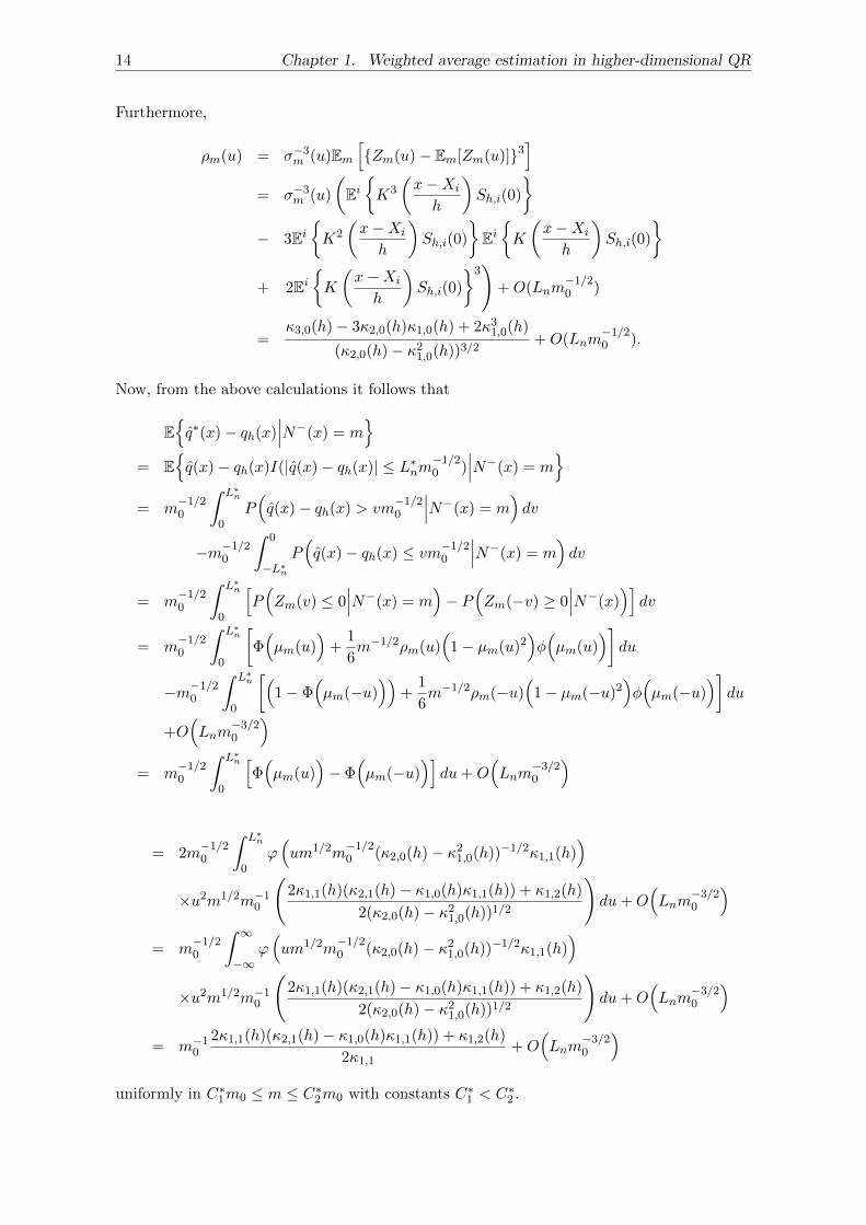
Now, from the above calculations it follows that
E{q∗(x)− qh(x)
∣∣∣N−(x) = m}
= E{q(x)− qh(x)I(|q(x)− qh(x)| ≤ L∗nm
−1/20 )
∣∣∣N−(x) = m}
= m−1/20
∫ L∗n
0P(q(x)− qh(x) > vm
−1/20
∣∣∣N−(x) = m)dv
−m−1/20
∫ 0
−L∗n
P(q(x)− qh(x) ≤ vm−1/20
∣∣∣N−(x) = m)dv
= m−1/20
∫ L∗n
0
[P(Zm(v) ≤ 0
∣∣∣N−(x) = m)− P
(Zm(−v) ≥ 0
∣∣∣N−(x))]dv
= m−1/20
∫ L∗n
0
[Φ(µm(u)
)+
1
6m−1/2ρm(u)
(1− µm(u)2
)φ(µm(u)
)]du
−m−1/20
∫ L∗n
0
[(1− Φ
(µm(−u)
))+
1
6m−1/2ρm(−u)
(1− µm(−u)2
)φ(µm(−u)
)]du
+O(Lnm
−3/20
)= m
−1/20
∫ L∗n
0
[Φ(µm(u)
)− Φ
(µm(−u)
)]du+O
(Lnm
−3/20
)
= 2m−1/20
∫ L∗n
0ϕ(um1/2m
−1/20 (κ2,0(h)− κ21,0(h))−1/2κ1,1(h)
)×u2m1/2m−10
(2κ1,1(h)(κ2,1(h)− κ1,0(h)κ1,1(h)) + κ1,2(h)
2(κ2,0(h)− κ21,0(h))1/2
)du+O
(Lnm
−3/20
)= m
−1/20
∫ ∞−∞
ϕ(um1/2m
−1/20 (κ2,0(h)− κ21,0(h))−1/2κ1,1(h)
)×u2m1/2m−10
(2κ1,1(h)(κ2,1(h)− κ1,0(h)κ1,1(h)) + κ1,2(h)
2(κ2,0(h)− κ21,0(h))1/2
)du+O
(Lnm
−3/20
)= m−10
2κ1,1(h)(κ2,1(h)− κ1,0(h)κ1,1(h)) + κ1,2(h)
2κ1,1+O
(Lnm
−3/20
)uniformly in C∗1m0 ≤ m ≤ C∗2m0 with constants C∗1 < C∗2 .
1.3. Proof of Theorem 1.1 15
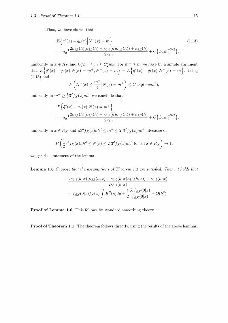
Thus, we have shown that
E{q∗(x)− qh(x)
∣∣∣N−(x) = m}
(1.13)
= m−10
2κ1,1(h)(κ2,1(h)− κ1,0(h)κ1,1(h)) + κ1,2(h)
2κ1,1+O
(Lnm
−3/20
),
uniformly in x ∈ RX and C∗1m0 ≤ m ≤ C∗2m0. For m+ ≥ m we have by a simple argument
that E{q∗(x) − qh(x)
∣∣∣N(x) = m+, N−(x) = m}
= E{q∗(x) − qh(x)
∣∣∣N−(x) = m}
. Using
(1.13) and
P
(N−(x) ≤ m+
4
∣∣∣N(x) = m+
)≤ C exp(−cnhd),
uniformly in m+ ≥ 123dfX(x)nhd we conclude that
E{q∗(x)− qh(x)
∣∣∣N(x) = m+}
= m−10
2κ1,1(h)(κ2,1(h)− κ1,0(h)κ1,1(h)) + κ1,2(h)
2κ1,1+O
(Lnm
−3/20
),
uniformly in x ∈ RX and 123dfX(x)nhd ≤ m+ ≤ 2 3dfX(x)nhd. Because of
P
(1
23dfX(x)nhd ≤ N(x) ≤ 2 3dfX(x)nhd for all x ∈ RX
)→ 1,
we get the statement of the lemma.
Lemma 1.6 Suppose that the assumptions of Theorem 1.1 are satisfied. Then, it holds that
2κ1,1(h, x)(κ2,1(h, x)− κ1,0(h, x)κ1,1(h, x)) + κ1,2(h, x)
2κ1,1(h, x)
= fε|X(0|x)fX(x)
∫K2(u)du+
1
2
∂εfε|X(0|x)
fε|X(0|x)+O(h2).
Proof of Lemma 1.6. This follows by standard smoothing theory.
Proof of Theorem 1.1. The theorem follows directly, using the results of the above lemmas.
References, chapter 1
Belloni, Alexandre, Victor Chernozhukov, and Ivan Fernandez-Val (2011). “Conditionalquantile processes based on series or many regressors”. In:
Chaudhuri, Probal (1991). “Nonparametric estimates of regression quantiles and their localBahadur representation”. In: The Annals of statistics 19.2, pp. 760–777.
Chaudhuri, Probal, Kjell Doksum, and Alexander Samarov (1997). “On average derivativequantile regression”. In: The Annals of Statistics 25.2, pp. 715–744.
Dette, Holger and Stanislav Volgushev (2008). “Non-crossing non-parametric estimates ofquantile curves”. In: Journal of the Royal Statistical Society: Series B (Statistical Method-ology) 70.3, pp. 609–627.
El Ghouch, Anouar and Ingrid Van Keilegom (2009). “Local linear quantile regression withdependent censored data”. In: Statistica Sinica, pp. 1621–1640.
Guerre, Emmanuel and Camille Sabbah (2012). “Uniform bias study and Bahadur represen-tation for local polynomial estimators of the conditional quantile function”. In: Econo-metric Theory 28.01, pp. 87–129.
Hardle, Wolfgang and Thomas M Stoker (1989). “Investigating smooth multiple regressionby the method of average derivatives”. In: Journal of the American Statistical Association84.408, pp. 986–995.
He, Xuming and Pin Ng (1999). “Quantile splines with several covariates”. In: Journal ofStatistical Planning and Inference 75.2, pp. 343–352.
He, Xuming, Pin Ng, and Stephen Portnoy (1998). “Bivariate quantile smoothing splines”. In:Journal of the Royal Statistical Society: Series B (Statistical Methodology) 60.3, pp. 537–550.
Hoderlein, Stefan and Enno Mammen (2009). “Identification and estimation of local aver-age derivatives in non-separable models without monotonicity”. In: The EconometricsJournal 12.1, pp. 1–25.
Hong, Sheng-Yan (2003). “Bahadur representation and its applications for local polynomialestimates in nonparametric M-regression”. In: Journal of Nonparametric Statistics 15.2,pp. 237–251.
Koenker, Roger (2005). Quantile regression. Cambridge university press.Koenker, Roger and Gilbert Bassett Jr (1978). “Regression quantiles”. In: Econometrica:
journal of the Econometric Society, pp. 33–50.Koenker, Roger, Pin Ng, and Stephen Portnoy (1994). “Quantile smoothing splines”. In:
Biometrika 81.4, pp. 673–680.Kong, Efang, Oliver Linton, and Yingcun Xia (2010). “Uniform Bahadur representation for
local polynomial estimates of M-regression and its application to the additive model”.In: Econometric Theory 26.05, pp. 1529–1564.
Lee, Young Kyung and Eun Ryung Lee (2008). “Kernel methods for estimating derivativesof conditional quantiles”. In: Journal of the Korean Statistical Society 37.4, pp. 365–373.
16

REFERENCES, CHAPTER 1 17
Li, Qi and Jeffrey S Racine (2008). “Nonparametric estimation of conditional CDF andquantile functions with mixed categorical and continuous data”. In: Journal of Business& Economic Statistics 26.4, pp. 423–434.
Mammen, Enno, Ingrid Van Keilegom, and Kyusang Yu (2015). “Expansion for moments ofregression quantiles with application to nonparametric testing”. In: Working Paper.
Portnoy, Stephen (1997). “Local asymptotics for quantile smoothing splines”. In: The Annalsof Statistics, pp. 414–434.
Roy, Arati et al. (1976). “The structure of degraded bael (Aegle marmelos) gum”. In: Car-bohydrate Research 50.1, pp. 87–96.

Chapter 2
Endogenous Shocks in Social
Networks: Effects of Students’
Exam Retakes on their Friends’
Future Performance
2.1 Introduction
The peer effect, the effect that social connections have on people’s behavior and
achievements, plays an important role when analyzing educational outcomes. While there
are numerous economics papers on peer effects across many fields, from education to juve-
nile behavior, the effect of shocking events on the friends network is rarely discussed. In
particular, in the university framework, students’ failures, such as retakes of examinations
or dropouts are usually only discussed for the students’ results in the same year and not in
relation to their friends’ future behaviour. However, the shock of a friend’s failure influences
the future behaviour and outcomes, especially when this failure was not anticipated.
This project contributes to the literature by covering an existing gap in peer effects
literature and studying the changes of peers’ behaviour and achievement in response to the
individual shock. In contrast to some examples in development literature (e.g. Comola and
Prina (2014)) considering exogenous individual treatment, I propose the model, allowing
the shock to be endogenously formed. Two components of the shock can be disentangled:
predicted probability of the shock and unexpected component. The latter is considered to
be crucial to the changes of future behavior. I am considering the students’ exam failure as
the source of the shock and test the model on the sample of students of one cohort at the
National Research University - Higher School of Economics, a highly selective university in
Russia. The threat of retakes and dropouts may put a lot of pressure on students, and the
higher probability of failure may result in lower productivity. Knowing, how these shocks
18
2.1. Introduction 19
influence the behavior of the students and their friends, can help to understand the whole
dynamics of network performance, and maybe help universities to adjust the strategy of set-
ting up the retakes’ threshold. Of course, dropouts are likely to influence future behaviour
stronger than retakes, since the latter can still be fixed. However, the existing data of the
dropouts is not sufficient for proper econometric analysis. I discuss both sources of shock in
descriptive analysis but apply the econometric model only to retakes.
The direction of the effect, however, can be twofold. While the unexpected shock
may serve as a wake-up call and motivate students to be more dedicated to their studies,
the connections can be extremely tight. This can reduce the amount of time spent on one’s
own studies due to the shared activities with the friend either outside of the university, if
the friend left, or helping the friend to prepare for the retake of the exam. The reasons of
the retakes during the studies can be different. In the first year, students are more likely to
fail due to the lack of the abilities or difficulties with adjustments to the new environment.
The fist exams may appear to be too difficult for some of the students, even though they had
sufficient abilities to enter the university. Students with lower abilities are either dropping
out of the university or adjusting their efforts to improve performance. In the second and
higher year, students are more likely to fail due to insufficient efforts. Therefore, the shock
during the different time periods may have a different effect on the future performance. This
paper discusses only the first year retakes at the moment.
Although I do not study the pure peer effect in this paper, I exploit the general
idea of peer effects literature and its methodological fundamentals. Most of the economic
literature that analyses peer effects use the framework and the model introduced by Manski
(1993). He distinguishes three effects that determine the similar behaviour of peers. The
endogenous effect explains that the probability of a particular student to drop out of the
school or university or to fail an exam will be affected by a number of this student’s peers
who have already done so. The exogenous effect uses mean exogenous characteristics of the
peer group, such as parental education, socio-economic status (SES), etc., to determine the
probability of the dropout or retake. The correlated effect appears due to the similar indi-
vidual characteristics within a group. The most important task of peer effects analysis is to
determine the endogenous effect, which can have important policy implications.
Identification of these three effects in the case of group interactions requires an
additional source of exogenous variation, such as exogenous class formation (for example,
Carrell, Fullerton, and West, 2009 in military institutions framework and De Giorgi, Pel-
lizzari, and Redaelli (2010) and Androushchak, Poldin, and Yudkevich (2013) in university
frameworks with randomly assigned groups) or random assignment of dormmates (for exam-
ple, B. Sacerdote, 2011). Estimating the endogenous peer effect as an effect of an average
group performance obtained some critique, and additional assumptions on the structure or
the ranking inside the peer group or even exact links are preferable, but social network data
is not always available. Usage of social network data requires other identifying assumptions,
which restrict the network. Bramoulle, Djebbari, and Fortin (2009) proved the identification
of the peer effect in social networks under rather mild assumptions. Poldin, Valeeva, and
Yudkevich (2015) use the same identification result to study the peer effect in the university
20 Chapter 2. Endogenous Shocks in Social Networks
framework using HSE dataset.
The identification of the direct effect of shock on the friends’ future outcome is,
however, more challenging, since the changes of the performance are not driven solely by the
effects of the shocks. Exogenous and unobserved characteristics of the student and his peers
as well as the changes in the network structure are among the other determinants. More-
over, as was already mentioned, the shock itself is not exogenous, and its significant part is
driven by the model itself. The paper proposes an econometric model which deals with both
problems and estimates the effect of the shock: a two-step dynamic peer effects model. The
first step estimates the probability of the shock adopting the instrumental variable 2SLS
approach discussed by Bramoulle, Djebbari, and Fortin (2009) after L. Lee (2003). The
second step uses the residuals from the first stage to estimate the effect of the unexpected
component of the changes in students’ performance.
To the best of my knowledge, this project is the first to introduce the dynamic
peer effect in social networks model with endogenous shock1. Moreover, I provide the iden-
tification results for this model and propose estimation procedure. The identification and
estimation of the first step are the straightforward adjustments of the Bramoulle, Djebbari,
and Fortin (2009) approach, and requires the existence of intransitive triads in the network
given the assumption of no correlated effects, i.e. friends of some student’s friends not con-
nected to him or her. Hence, the friends of friend affect the student not directly, but via
the common friend only. If the assumption of no correlated effects is relaxed, the stricter
identifying assumption is necessary. The whole network should include pairs of students with
the distance between them of length three or bigger. They are not connected directly, and
the shortest path from the one to the other has not less than three links. Friends of friends
are used to deal with the correlated effect, therefore, the next level of friends is used as an
identifying assumption. The identification of the second step is novel and demonstrates the
necessity of the network longitudinal variation. Changes of the network allow comparing the
influence of ”old” and ”new” peer group on the outcome. The presence of the new friends
and absence of old ones creates variation in the peer group characteristics and this helps to
identify social effects and the effect of the shock. However, it is important that the changes
of the network are not driven solely by the shock. Moreover, at the moment, I do not model
link formation, and therefore, do not distinguish between different types of network changes
and treat them all as equal and given.
The variation of the network is a valid assumption for the students’ network setting.
The links formed in the first year are highly likely to be revised due to the gradual unveiling
of the friends’ personal characteristics. Some of the links might be broken, however, due to
the exam retakes and dropouts of the friends. The student may seek for a more advantageous
peer group or he/she no longer spends much time with the friend preparing for the retakes.
But even if the friend fails an exam and the link stays stable in the network, the student may
tend to connect to the students with higher results, creating new links. The exam retake
is endogenous in the model, and only an unexpected component of the retake probability is
1See, for example, a review of the recent econometric literature on networks in Paula (2015)
2.2. Model 21
considered as a shock. The influence of this unexpected component on link formation is not
the same as possible channels of influence of retakes on link formation, discussed previously,
therefore, the actual importance of the shock for link changes might be lower than the one
of exam retakes. The model in the paper is discussed without link formation process and,
therefore, under the assumption that changes in the network are exogenously given. This
setup is a bit restrictive, and relaxation of this assumption will be considered for future
research.
The magnitude of the endogenous effects in different periods is considered to be
different, since the unexpected shock may affect performance via the changes of the peer
groups, and not only directly. The break of the link itself makes the peer group ”better”,
then the improvement of the results can also be caused by the group’s refinement.
Dropouts and retakes are important to study from the university’s perspective.
Dropouts create the sunk costs for the university. For example, costs of the university
dropouts in Germany were estimated at the level of $11.5 billion in 20072 and in Australia
at $1.36 billion3. Some of the dropouts are the results of the policies of the university, which
can be controlled. In some institutions of higher education, as in the sample used in the
analysis, most of the dropouts are directly affected by the retakes. In HSE 3 retakes during
the same exam session term will lead to the expulsion of the student. Therefore, under-
standing the possible mechanisms of retakes’ influence on future performance may suggest
possible university-level policy improvements in order to reduce sunk costs.
The paper is organized as follows. Section 2 discusses the proposed model, states
the identifying assumptions, and proposes the estimation method. Section 3 describes the
data used and the institutional environment of the educational system in Russia, as well as
results of the descriptive analysis. Section 4 provides the estimation results and evidence of
the influence of dropouts and retakes on peers. Section 5 concludes.
2.2 Model
2.2.1 Naıve approach
I propose a two-step model that allows estimating the effect of an unexpected event
happening to network connections. Although I do not conduct the pure peer effect estima-
tion, I use the classical peer effect model as a baseline.
A naıve way to write down the dynamic peer effect model without modelling the link forma-
tion:
y1i = α1 + β1∑j 6=i
G1ijy
1j + γ1X
1i + δ1
∑j 6=i
G1ijX
1j + ξi + ε1i , E[ε1i |X1] = 0, (2.1)
2The figures are obtained by the Stifterverband, association of German science and higher educationdonors. Details can be found on UWN website
3According to the report on UWN website
22 Chapter 2. Endogenous Shocks in Social Networks
y2i = α2 + β2∑j 6=i
G2ijy
2j + γ2X
2i + δ2
∑j 6=i
G2ijX
2j + ξi + ε2i , E[ε2i |X2] = 0, (2.2)
where y1i and y2i are outcome variables of student i in the first wave and the second wave
correspondingly. I will consider the average grade in the main specification of the model.
Student’s rating or grades for some specific subjects, which last more than 1 term, are used
for robustness checks;
Xi is a vector of individual characteristics that should be controlled for, such as gender,
city of origin, living conditions, some socioeconomic family characteristics. In the discussed
empirical example it also includes the results of the high school examination, universal and
obligatory for all the students graduating the high school.
G1ij and G2
ij are two adjacency matrices for the first and the second waves correspondingly,
weighted by the number of links, and their entries have the value of 1/ni if the link from
student i to student j exists. Note that this matrices are not necessarily symmetrical, since
the social network can be both directed (as in the sample used later) or undirected.
ξi - student-level unobserved fixed characteristics, which may influence students’ performance
and choice of connections.
Those unobserved individual characteristics also reflect the homophily of the indi-
viduals, which may influence both link formation and the network outcomes. In the case
of group interactions group fixed effects are often introduced to eliminate correlated effects,
whereas in the case of interactions in big networks network fixed effects make little sense. Lo-
cal differences, proposed by Bramoulle, Djebbari, and Fortin (2009), may be used to address
the issue of correlated effects. However, the dynamic structure of the data allows solving this
issue differently. The dynamic peer model can be then written in terms of differences, and
this will eliminate possible unobserved fixed effect component in the error term, consisting
of the common for individual’s connections unobservable component and individual’s own
unobserved fixed characteristics.
∆yi = ∆α+ β2∑j 6=i
G2ijy
2j − β1
∑j 6=i
G1ijy
1j + γ2X
2i − γ1X1
i + δ2∑j 6=i
G2ijX
2j − δ1
∑j 6=i
G1ijX
1j + ∆εi
Assumption A. The outcome variable of a single period can be estimated using the
one-period model.
This additional assumption allows avoiding the autoregressive component in the
second-period model. Assumption A is valid, because the model, including observed and
unobserved fixed effects characteristics as well as endogenous and exogenous peer effects, is
sufficient to predict the educational achievements. Therefore, it can be claimed that there is
no additional mechanism that can influence the outcome via the previous period’s outcome.
The proposed model system 2.1 and 2.2, and consequently, the model written in
differences, can be further modified in order to catch the desirable effect of shock. In the
naıve way, similar to the model of Comola and Prina (2014), the model will now be as follows:
2.2. Model 23
The equation for the first period should remain unchanged:
y1i = α1 + β1∑j 6=i
G1ijy
1j + γ1X
1i + δ1
∑j 6=i
G1ijX
1j + ξi + ε1i ,
Whereas, the second-period model shall take into account the shock of unexpected
retake of the friend. The straightforward way to do it is just to include the binary variable
in the vector of controls:
y2i = α2 + β2∑j 6=i
G2ijy
2j + δDi + γ2X
2i + δ2
∑j 6=i
G2ijX
2j + ξi + ε2i
where Di is a dummy for having any friends with a retake in the first period4.
The system can then be re-written in differences, eliminating the possible individual
fixed effect:
∆yi = (α2 − α1) + β2∑j 6=i
G2ijy
2j − β1
∑j 6=i
G1ijy
1j + γDi +
+γ2X2i − γ1X1
i + δ2∑j 6=i
G2ijX
2j − δ1
∑j 6=i
G1ijX
1j + ε2i − ε1i
However, this type of the equation is only valid if the shock is exogenous, as in the
examples of randomized treatment. A big share of the probability of the student’s retake
can be explained by the observed component of the model, and therefore, the retake itself
cannot be considered as unexpected shock. I propose to use the peer effect model of the first
period to disentangle predictable and unexpected parts of the probability of the retake, and
use the unpredicted part only to estimate the effect of the shock on the performance.
Comola and Prina (2014) also model the changes of the network as a response to the
exogenous treatment. At the moment, I am not modelling the link formation. The variation
of the network links is assumed and is a crucial identifying assumption. Importantly, a
significant part of the changes in the structure of the friendship networks is caused by the
individual characteristics and outcome and not solely by the exam retake. The influence
of the retake and of the unpredicted component of the retake on the link formation also
should be treated and interpreted differently, since the probability of the exam retake is
endogenous. The following assumption, therefore, should be made. Assumption B. Changes
of the network as a response to unexpected shock are neglected, and all changes of the
network itself are treated as exogenous.
This assumption can potentially cause overestimation of the direct effect of the
shock, and therefore, should be relaxed in the future research.
4In general the coefficients in the model with the shock are different from the baseline one-period models(1) and (2), but I left the same notations for simplicity
24 Chapter 2. Endogenous Shocks in Social Networks
2.2.2 Proposed model with no correlated effects
The model
Taking into account all above-mentioned argument, I estimate the following model
at the first step:
P (retakei) = α+ β∑j 6=i
G1ijy
1j + γX1
i + δ∑j 6=i
G1ijX
1j + ξi + νi, E[νi|X1] = 0 (2.3)
In this specification, the error term consists of two parts: unobserved correlated effect, and
conditionally independent noise. Dynamic peer effect model will eliminate the correlated
effect component at the second step of the model, leading to the conditional independence
of the error term. However, on the first step in general E[ξi + νi|X1] 6= 0. I will discuss two
cases: assuming no correlated effects and with correlated effect. The latter will be considered
in the later subsections. For the former, 2.3 will be transformed as follows :
P (retakei) = α+ β∑j 6=i
G1ijy
1j + γX1
i + δ∑j 6=i
G1ijX
1j + νi, E[νi|X1] = 0 (2.3a)
I then take the residuals of the equation 2.3a, which is the part of the probability of
the friends’ retake not predicted by the model. I then construct the shock for student i as the
combination of the residuals for the students in the network of i. The baseline specification
uses the average of the residuals: URi =∑
j 6=iG1ij νj . However, the other approaches to
define URi is possible: maximum of friends’ unpredicted probability of the exam retakes,
residuals for the friends named first, or average weighted according to the order, with which
friends are appearing in the answers of the students. The identification results and estimation
procedure are not affected by the choice of the approach to defining URi. Then I am using
it as an unexpected shock to plug-in in the following equation:
∆yi = (α2 − α1) + β2∑j 6=i
G2ijy
2j − β1
∑j 6=i
G1ijy
1j + δURi + γ2X
2i − γ1X1
i +
+ δ2∑j 6=i
G2ijX
2j − δ1
∑j 6=i
G1ijX
1j + ∆εi (2.4)
Since the model in differences eliminates possible individual fixed effect component in error
term, I am able to make a stricter assumption on the error term: E[∆εi] = 0, instead of the
conditional expectation. This condition will be used to prove the model identification.
Model in differences, additional to the elimination of individual fixed effect, gives a
better interpretation of the studied effect. It estimates the changes of own performance in
response to the shock additional to the changes of performance in comparison to the class-
mates, obtained by the single-period model.
Note that the coefficients for the endogenous peer effect and exogenous characteris-
tics are considered to be different in two periods: β2 and β1 and δ2 and δ1. Students may
2.2. Model 25
experience the different magnitude of the effects depending on how advanced they are in their
studies, how well they are adjusted to the university environment, etc. Moreover, this also
allows to take into account the changes in the network, since the students are experiencing
the influence of two different peer groups in two periods.
The own retake of the student is not included explicitly in the model. The unex-
pected component for the students themselves is close to zero since they can anticipate most
of the retakes after writing the exam. Moreover, the outcome of the previous period partially
takes care of own retakes. Nonetheless, in the empirical analysis, I will also split the sample
and study the effect for those, who were retaking the exams, and for those, who were not,
to tackle down possible differences.
Identifying assumptions
The identification results for the first step of the model adopt Bramoulle, Djebbari,
and Fortin (2009) approach, whereas the result, obtained for the second stage, is, to the best
of my knowledge, a novel result for the literature.
Lemma 2.1 Let γ21 +δ21 6= 0 and β1 6= 05. If matrices I, G1, (G1)2 are linearly independent,
coefficients in 2.3a are identified.
The proof of Lemma 2.1 is given in Appendix A. This is exactly the condition obtained by
(Bramoulle, Djebbari, and Fortin, 2009), and can be proven similarly. The identification of
the coefficients on the first step, hence, allow using the obtained residuals for the further
analysis. The identification is ensured by the existence of intransitive triads in the network,
i.e. the existence of a set of three individuals i, j, k such that i is influenced by j, j is influ-
enced by k, but i is not influenced by k. This is a valid assumption for most networks, in
particular, for the sample analysed in this paper, which will be discussed in the next section.
Lemma 2.2 In the case of no correlated effects, if the assumptions of Lemma 2.1 hold, if
γ22 + δ22 6= 0 and β2 6= 06, if matrices I, G2, (G2)2 are linearly independent, and if G1 6= G2,
with changes not driven by the shock only, coefficients in 2.4 are identified.
Identification of Step 2 relies heavily on the variation in the network structure. However, it
is important that some changes in the network are exogenous. This assumption is quite rea-
sonable for the friendship networks. Students are likely to learn more about their classmates
with time, and the friendships, created during the first year, are often unstable.
Once there are new links formed in the next period, the variation between new and
old connections help to capture the effect of the changes in the average grade. For example,
5These are the coefficients from the baseline peer effect model 2.1.6The coefficients from the baseline peer effect model 2.2
26 Chapter 2. Endogenous Shocks in Social Networks
if a student i is no longer connected to student j, and therefore, is not affected by student
j, his performance can be evaluating in the two cases and the comparison of two results will
result in the effect of not having friend j, and hence, the social effects are easier to catch.
The identifying assumptions also put the restriction on the friendship matrix of the second
period, as in the first period: the network should include intransitive triads. The proof of
Lemma 2.2 can also be found in Appendix A, and the validity of identifying assumptions
will be discussed in the next Section.
2.2.3 Model with correlated effects
The model
As was already mentioned, the correlated effect appears due to the similar individual
characteristics within a group. The correlated effect is unlikely to be present in big networks,
however, once the network may suggest existence of smaller groups or subnetworks in it, the
correlated effects are more likely to be present. In the empirical application discussed in this
paper, most of the connections are formed inside of the same department, and even inside of
the same exogenously formed study group. Therefore, the possible correlated effects could
not be ignored and can cause an additional identification issue.
To deal with it and eliminate unobserved variables, I propose taking the local dif-
ferences, i.e. averaging the equation 2.3 over the friends of i and subtracting this average
from 2.3 and noting that ξi are the same for the students in one smaller network, and hence,
it will vanish after taking the local differences:
P (retakei)−∑j 6=i
G1ijP (retakej) = β
∑j 6=i
G1ij [y
1j −
∑k 6=j
G1jky
1k] + γ[X1
i −∑j 6=i
G1ijX
1j ]+
+ δ∑j 6=i
G1ij [X
1j −
∑j 6=k
G1jkX
1k ] + ηi, ηi = [νi −
∑j 6=i
G1ijνj ], E[ηi|X1] = 0 (2.5)
Similarly to the case without correlated effects, I construct the shock for the student
i, taking the average of their networks residuals: URi =∑
j 6=iG1ij ηj . The second stage is
then identical to the case with no correlated effects:
∆yi = (α2 − α1) + β2∑j 6=i
G2ijy
2j − β1
∑j 6=i
G1ijy
1j + δURi + γ2X
2i − γ1X1
i +
+ δ2∑j 6=i
G2ijX
2j − δ1
∑j 6=i
G1ijX
1j + ∆εi (2.6)
Model in differences, additional to the elimination of individual fixed effect, also gets
rid off the correlated effects, therefore, no local differences are needed for the second stage
equation.
2.2. Model 27
Identifying assumptions
The identification results for the first step of the model again adopt Bramoulle,
Djebbari, and Fortin (2009) approach, whereas the result, obtained for the second stage, is
new.
Lemma 2.3 Let γ21 + δ21 6= 0 and β1 6= 07. If matrices I, G1, (G1)2, (G1)3 are linearly
independent, coefficients in 2.5 are identified.
The proof is given in Appendix A. This condition again follows the result of (Bramoulle,
Djebbari, and Fortin, 2009) in the presence of correlated effects, and can be proven in the
similar manner. The identification of model with correlated effects is ensured by the exis-
tence of distances between two students of length 3 and more, i.e. the existence of a set of at
least 4 individuals i, j, k,m such that i is influenced by j, j is influenced by k, k is influenced
by m, but i is not influenced by both m and k, and j is not influenced by m. This is a bit
more demanding assumption than in the case of no correlated effects, but still valid for a lot
of networks’ types, and in particular, for the sampled network, which will be discussed in
the next section.
Lemma 2.4 In the case of correlated effects, if the assumptions of Lemma 2.3 hold, if
γ22 + δ22 6= 0 and β2 6= 08, if matrices I, G2, (G2)2, (G2)3 are linearly independent, and if
G1 6= G2, with changes not driven by the shock only, coefficients in 2.6 are identified.
Identification of Step 2 again heavily relies on the variation in the network structure. More-
over, the restrictions are put on the friendship matrix of the second period, requiring the
distances between two students of length 3 and more. The proof of Lemma 2.4 is presented
in Appendix A.
2.2.4 Estimation strategy
No correlated effects
I first discuss the model that does not take into account correlation effects: 2.3a and
2.4.
Step 1. I partially repeat Bramoulle, Djebbari, and Fortin (2009) for the first step and use
the adaptation of Generalized 2SLS strategy proposed by Kelejian and Prucha (1998) and
refined by L. Lee (2003). As the identification result suggests, ((G1)2X, (G1)3X, . . . ) can
be used as valid instruments to obtain consistent estimators.
7The coefficients from the baseline peer effect model 2.18The coefficients from the baseline peer effect model 2.2
28 Chapter 2. Endogenous Shocks in Social Networks
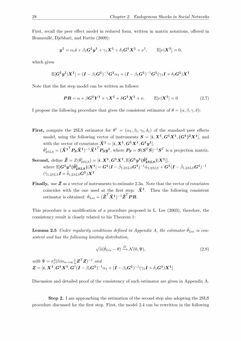
First, recall the peer effect model in reduced form, written in matrix notations, offered in
Bramoulle, Djebbari, and Fortin (2009):
y1 = α1i+ β1G1y1 + γ1X
1 + δ1G1X1 + ν1, E[ν|X1] = 0,
which gives
E[G1y1|X1] = (I − β1G1)−1G1α1 + (I − β1G1)−1G1(γ1I + δ1G1)X1
Note that the fist step model can be written as follows:
PR = α+ βG1Y 1 + γX1 + δG1X1 + ν, E[ν|X1] = 0 (2.7)
I propose the following procedure that gives the consistent estimator of θ = (α, β, γ, δ):
First, compute the 2SLS estimator for θ1 = (α1, β1, γ1, δ1) of the standard peer effects
model, using the following vector of instruments S = [i,X1,G1X1, (G1)2X1], and
with the vector of covariates X1 = [i,X1,G1X1,G1y1].
θ12SLS = (X1TPSX1)−1X1TPSy
1, where PS = S(STS)−1ST is a projection matrix.
Second, define Z = Z(θ12SLS) = [i,X1,G1X1,E[G1y1(θ12SLS)|X1]],
where E[G1y1(θ12SLS)|X1] = G1(I − β1,2SLSG1)−1α1,2SLS +G1(I − β1,2SLSG1)−1
(γ1,2SLSI + δ1,2SLSG1)X1
Finally, use Z as a vector of instruments to estimate 2.3a. Note that the vector of covariates
coincides with the one used at the first step: X1. Then the following consistent
estimator is obtained: θLee = (ZTX1)−1Z
TPR.
This procedure is a modification of a procedure proposed in L. Lee (2003), therefore, the
consistency result is closely related to his Theorem 1:
Lemma 2.5 Under regularity conditions defined in Appendix A, the estimator θLee is con-
sistent and has the following limiting distribution,
√n(θLee − θ)
D−→ N (0,Ψ), (2.8)
with Ψ = σ2ν(limn→∞1nZ
TZ)−1 and
Z = [i,X1,G1X1,G1(I − β1G1)−1α1 + (I − β1G1)−1(γ1I + δ1G1)X1]
Discussion and detailed proof of the consistency of such estimator are given in Appendix A.
Step 2. I am approaching the estimation of the second step also adopting the 2SLS
procedure discussed for the first step. First, the model 2.4 can be rewritten in the following
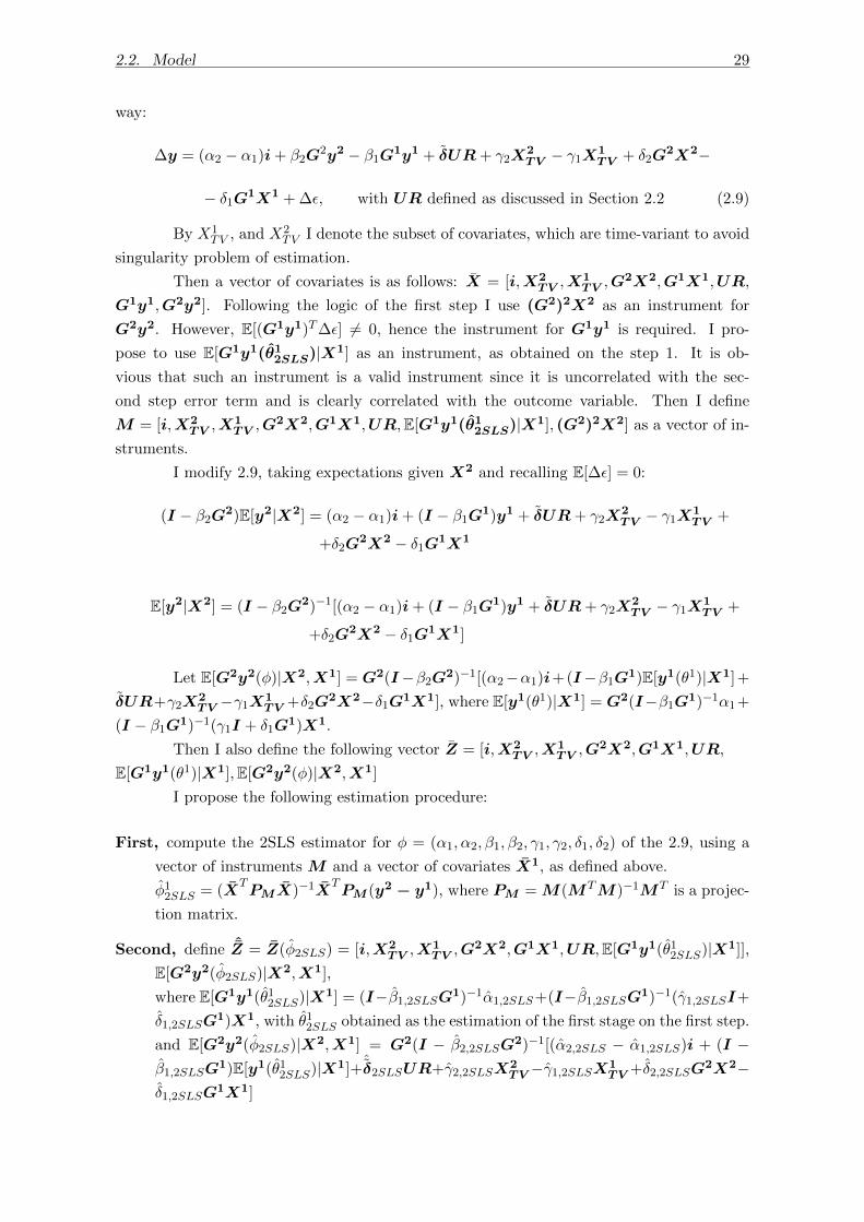
2.2. Model 29
way:
∆y = (α2 − α1)i+ β2G2y2 − β1G1y1 + δUR+ γ2X
2TV − γ1X
1TV + δ2G
2X2−
− δ1G1X1 + ∆ε, with UR defined as discussed in Section 2.2 (2.9)
By X1TV , and X2
TV I denote the subset of covariates, which are time-variant to avoid
singularity problem of estimation.
Then a vector of covariates is as follows: X = [i,X2TV ,X
1TV ,G
2X2,G1X1,UR,
G1y1,G2y2]. Following the logic of the first step I use (G2)2X2 as an instrument for
G2y2. However, E[(G1y1)T∆ε] 6= 0, hence the instrument for G1y1 is required. I pro-
pose to use E[G1y1(θ12SLS)|X1] as an instrument, as obtained on the step 1. It is ob-
vious that such an instrument is a valid instrument since it is uncorrelated with the sec-
ond step error term and is clearly correlated with the outcome variable. Then I define
M = [i,X2TV ,X
1TV ,G
2X2,G1X1,UR,E[G1y1(θ12SLS)|X1], (G2)2X2] as a vector of in-
struments.
I modify 2.9, taking expectations given X2 and recalling E[∆ε] = 0:
(I − β2G2)E[y2|X2] = (α2 − α1)i+ (I − β1G1)y1 + δUR+ γ2X2TV − γ1X
1TV +
+δ2G2X2 − δ1G1X1
E[y2|X2] = (I − β2G2)−1[(α2 − α1)i+ (I − β1G1)y1 + δUR+ γ2X2TV − γ1X
1TV +
+δ2G2X2 − δ1G1X1]
Let E[G2y2(φ)|X2,X1] = G2(I−β2G2)−1[(α2−α1)i+(I−β1G1)E[y1(θ1)|X1]+
δUR+γ2X2TV −γ1X1
TV +δ2G2X2−δ1G1X1], where E[y1(θ1)|X1] = G2(I−β1G1)−1α1+
(I − β1G1)−1(γ1I + δ1G1)X1.
Then I also define the following vector Z = [i,X2TV ,X
1TV ,G
2X2,G1X1,UR,
E[G1y1(θ1)|X1],E[G2y2(φ)|X2,X1]
I propose the following estimation procedure:
First, compute the 2SLS estimator for φ = (α1, α2, β1, β2, γ1, γ2, δ1, δ2) of the 2.9, using a
vector of instruments M and a vector of covariates X1, as defined above.
φ12SLS = (XTPMX)−1X
TPM (y2 − y1), where PM = M(MTM)−1MT is a projec-
tion matrix.
Second, define ˆZ = Z(φ2SLS) = [i,X2TV ,X
1TV ,G
2X2,G1X1,UR,E[G1y1(θ12SLS)|X1]],
E[G2y2(φ2SLS)|X2,X1],
where E[G1y1(θ12SLS)|X1] = (I−β1,2SLSG1)−1α1,2SLS+(I−β1,2SLSG1)−1(γ1,2SLSI+
δ1,2SLSG1)X1, with θ12SLS obtained as the estimation of the first stage on the first step.
and E[G2y2(φ2SLS)|X2,X1] = G2(I − β2,2SLSG2)−1[(α2,2SLS − α1,2SLS)i + (I −
β1,2SLSG1)E[y1(θ12SLS)|X1]+
ˆδ2SLSUR+γ2,2SLSX
2TV −γ1,2SLSX1
TV +δ2,2SLSG2X2−
δ1,2SLSG1X1]
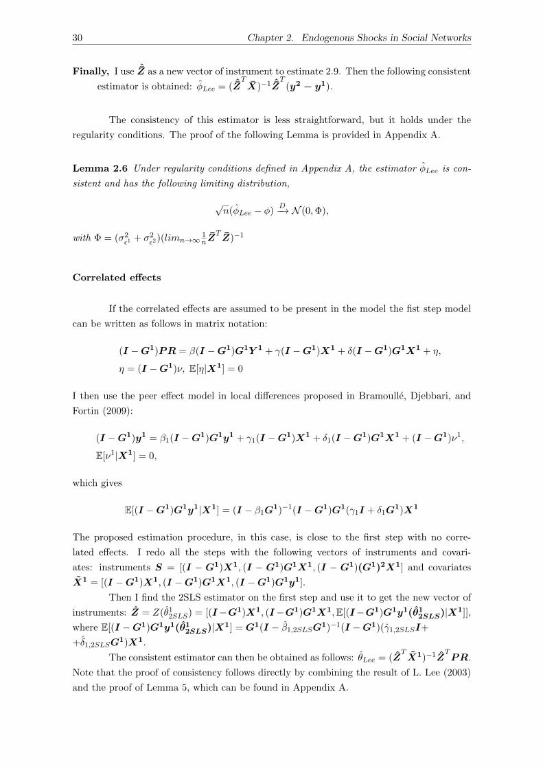
30 Chapter 2. Endogenous Shocks in Social Networks
Finally, I use ˆZ as a new vector of instrument to estimate 2.9. Then the following consistent
estimator is obtained: φLee = ( ˆZTX)−1 ˆZ
T(y2 − y1).
The consistency of this estimator is less straightforward, but it holds under the
regularity conditions. The proof of the following Lemma is provided in Appendix A.
Lemma 2.6 Under regularity conditions defined in Appendix A, the estimator φLee is con-
sistent and has the following limiting distribution,
√n(φLee − φ)
D−→ N (0,Φ),
with Φ = (σ2ε1 + σ2ε2)(limn→∞1nZ
TZ)−1
Correlated effects
If the correlated effects are assumed to be present in the model the fist step model
can be written as follows in matrix notation:
(I −G1)PR = β(I −G1)G1Y 1 + γ(I −G1)X1 + δ(I −G1)G1X1 + η,
η = (I −G1)ν, E[η|X1] = 0
I then use the peer effect model in local differences proposed in Bramoulle, Djebbari, and
Fortin (2009):
(I −G1)y1 = β1(I −G1)G1y1 + γ1(I −G1)X1 + δ1(I −G1)G1X1 + (I −G1)ν1,
E[ν1|X1] = 0,
which gives
E[(I −G1)G1y1|X1] = (I − β1G1)−1(I −G1)G1(γ1I + δ1G1)X1
The proposed estimation procedure, in this case, is close to the first step with no corre-
lated effects. I redo all the steps with the following vectors of instruments and covari-
ates: instruments S = [(I − G1)X1, (I − G1)G1X1, (I − G1)(G1)2X1] and covariates
X1 = [(I −G1)X1, (I −G1)G1X1, (I −G1)G1y1].
Then I find the 2SLS estimator on the first step and use it to get the new vector of
instruments: Z = Z(θ12SLS) = [(I−G1)X1, (I−G1)G1X1,E[(I−G1)G1y1(θ12SLS)|X1]],
where E[(I −G1)G1y1(θ12SLS)|X1] = G1(I − β1,2SLSG1)−1(I −G1)(γ1,2SLSI+
+δ1,2SLSG1)X1.
The consistent estimator can then be obtained as follows: θLee = (ZTX1)−1Z
TPR.
Note that the proof of consistency follows directly by combining the result of L. Lee (2003)
and the proof of Lemma 5, which can be found in Appendix A.
2.3. Data and Descriptive analysis 31
Step 2 also requires some adjustments in this case. Due to the presence of corre-
lated effects, E[G1y1(θ12SLS)|X1] is no longer observable since it includes the unobserved
fixed effects correlated with covariates and cannot be used as an instrument. Hence, I need
to modify both vectors of covariates and instruments in the following way: X = [(I −G1)X2
TV , (I−G1)X1TV , (I−G1)G2X2, (I−G1)G1X1, (I−G1)UR, (I−G1)G1y1, (I−
G1)G2y2] is a new vector of covariates. I then use (I − G1)(G2)2X2 as an instru-
ment for (I − G1)G2y2. I propose to use E[(I −G1)G1y1(θ12SLS)|X] as an instru-
ment for (I − G1)G1y1. This instrument is clearly a valid instrument since it is uncor-
related with the second step error term and is clearly correlated with the outcome variable.
Then I define M = [(I − G1)X2TV , (I − G1)X1
TV , (I − G1)G2X2, (I − G1)G1X1, (I −G1)UR,E[(I −G1)G1y1(θ12SLS)|X], (I −G1)(G2)2X2] as a vector of instruments.
Applying the same changes to all relevant vectors, I then fully repeat the estimation
procedure of the case of no correlated effects, and obtain the consistent estimator. Consis-
tency of the estimator is achieved by the argument similar to the one in Lemma 2.6, proof of
which and more detailed discussion on estimation procedure can be found in Appendix A.
2.3 Data and Descriptive analysis
2.3.1 The system of higher education in Russia and specifics of the sam-
pled university.
People with completed full vocational education or completed professional education
of non-university level are eligible to enter the university9. Most of the places in the state
universities are financed by the government: around 65%10, but it differs among institutions.
For example, the analysed in this paper university, National State University - Higher School
of Economics, Nizhny Novgorod branch, provided 340 state-financed places out of total 431
in 201211. The tuition fee varies from institution to institution, in our example, it varies
between 130000 and 165000 Rubles, which equals to 28-36 times the minimum monthly wage
or 18-23 times the minimum cost of living in Russia.
The students are accepted to the universities depending on the scores of the obliga-
tory standardized examination, Unified School Examination, conducted at the end of the last
school year. Each high school graduate has to take the exam in several subjects: Mathemat-
ics and Russian are mandatory to graduate from the school, the other subjects are chosen by
the graduates depending on their preferences and the requirements of the universities they
are aiming to apply to. For example, economic department of NRU-HSE requires the USE
results in Social Studies (a mixture of basic knowledge about different aspects of society:
philosophy, sociology, social psychology, law, political science) and Foreign language addi-
9It is more accurate to call them the institutions of tertiary or post-secondary education, since not all ofthese institutions in Russia have the status of the university, however, the university will be used for simplicity
10According to the Monitoring of education markets and organizations (MEMO), NRU HSE. In Russian11The main dataset uses 2012 cohort of students, details are described in the next subsection
32 Chapter 2. Endogenous Shocks in Social Networks
tional to the mandatory to all graduates Mathematics and Russian. However, regional and
national level Olympiads can often be used as the second channel to enter some of the uni-
versities. These Olympiads are subject-specific and considered to be more sophisticated than
the school exams, so they are designed to attract more talented students. In Higher School of
Economics, the winners and prize-takers of these competitions are accepted to the university
without exams if the major of the Olympiads corresponds to the university department (Eco-
nomic Olympiads for economics department, Entrepreneurship Olympiads for management
department etc.) or automatically given the highest score for the other subjects. However,
those students are still required to take the USE and have the scores not lower than the
required minimum (65 out of 100 in 2015, significantly lower than the requirement to be
accepted). The share of students entering universities using the Olympiads results is around
5-6% overall in Russia, but it is much higher for the Higher School of Economics, around
40%, because of the selective status of HSE. Therefore, in general, the group of students
entering HSE is more or less homogeneous and consists of the high-achievers. Even though
Nizhniy Novgorod branch of HSE is less selective than the main Moscow branch, the level of
the admitted students is still very high. The list of all accepted students is publicly available
in the university itself as well as on the website.
Usually, universities in Russia have an exogenous group formation. The students
are randomly split into groups of 20-30 people before the beginning of the studies. These
groups stay mainly intact for the first three years. Several groups or even all students at-
tend lectures together, whereas each group has separate tutorials. The changes to the group
structure may occur if a lot of the students leave the university and the group is too small.
Most of the universities have by now adopted the Bologna Process model of 4 years for
Bachelor’s degree and 1-2 years of Master’s degree. In most cases each academic year has 2
terms with exams periods after each, however, HSE has 4 terms per year, with some exams
or pass-fail exams after the 1st and the 3rd term and with most exams after the 2nd and the
4th term. The student is not allowed to fail 3 or more exams per half (1+2 or 3+4 term)
and the retakes are conducted only after the 2nd and 4th exam periods of each year. All
results of all students are publicly available near the students’ office in the university and
online so that everybody can follow their own performance, compare to the peers, and the
tuition students can understand, whether they are eligible for the tuition discount.
2.3.2 Data description
The data is based on two longitudinal studies of the students’ network, conducted
in the National Research University Higher School of Economics (Nizhny Novgorod branch;
state university). The information about the studies is summarized in Table 2.1.
Table 2.1: Studies characteristics
Study Cohort Frequency Departments Total students
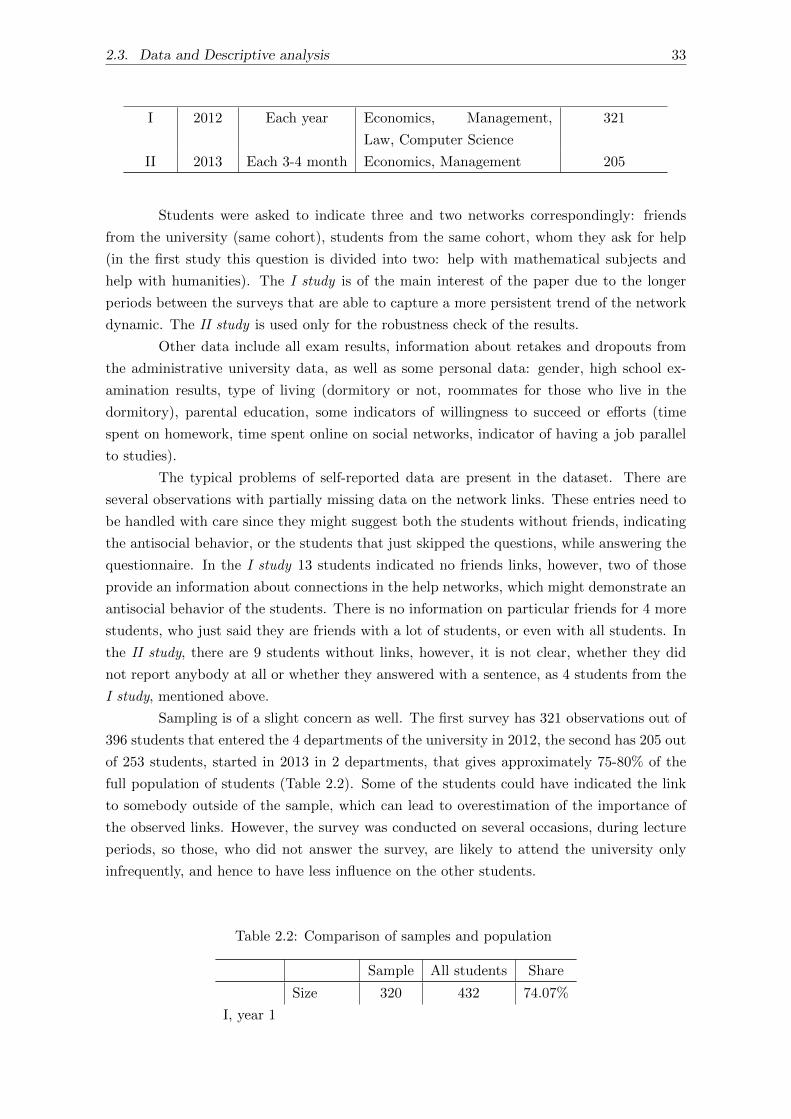
2.3. Data and Descriptive analysis 33
I 2012 Each year Economics, Management,
Law, Computer Science
321
II 2013 Each 3-4 month Economics, Management 205
Students were asked to indicate three and two networks correspondingly: friends
from the university (same cohort), students from the same cohort, whom they ask for help
(in the first study this question is divided into two: help with mathematical subjects and
help with humanities). The I study is of the main interest of the paper due to the longer
periods between the surveys that are able to capture a more persistent trend of the network
dynamic. The II study is used only for the robustness check of the results.
Other data include all exam results, information about retakes and dropouts from
the administrative university data, as well as some personal data: gender, high school ex-
amination results, type of living (dormitory or not, roommates for those who live in the
dormitory), parental education, some indicators of willingness to succeed or efforts (time
spent on homework, time spent online on social networks, indicator of having a job parallel
to studies).
The typical problems of self-reported data are present in the dataset. There are
several observations with partially missing data on the network links. These entries need to
be handled with care since they might suggest both the students without friends, indicating
the antisocial behavior, or the students that just skipped the questions, while answering the
questionnaire. In the I study 13 students indicated no friends links, however, two of those
provide an information about connections in the help networks, which might demonstrate an
antisocial behavior of the students. There is no information on particular friends for 4 more
students, who just said they are friends with a lot of students, or even with all students. In
the II study, there are 9 students without links, however, it is not clear, whether they did
not report anybody at all or whether they answered with a sentence, as 4 students from the
I study, mentioned above.
Sampling is of a slight concern as well. The first survey has 321 observations out of
396 students that entered the 4 departments of the university in 2012, the second has 205 out
of 253 students, started in 2013 in 2 departments, that gives approximately 75-80% of the
full population of students (Table 2.2). Some of the students could have indicated the link
to somebody outside of the sample, which can lead to overestimation of the importance of
the observed links. However, the survey was conducted on several occasions, during lecture
periods, so those, who did not answer the survey, are likely to attend the university only
infrequently, and hence to have less influence on the other students.
Table 2.2: Comparison of samples and population
Sample All students Share
I, year 1
Size 320 432 74.07%
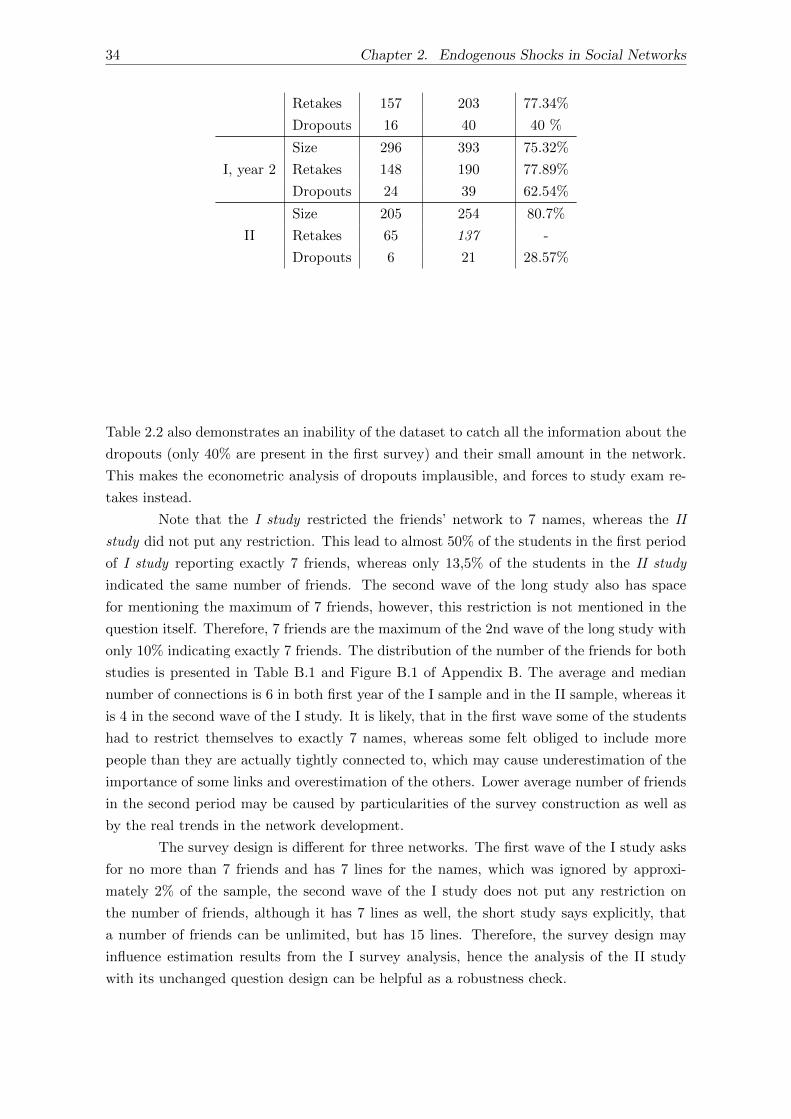
34 Chapter 2. Endogenous Shocks in Social Networks
Retakes 157 203 77.34%
Dropouts 16 40 40 %
I, year 2
Size 296 393 75.32%
Retakes 148 190 77.89%
Dropouts 24 39 62.54%
II
Size 205 254 80.7%
Retakes 65 137 -
Dropouts 6 21 28.57%
Table 2.2 also demonstrates an inability of the dataset to catch all the information about the
dropouts (only 40% are present in the first survey) and their small amount in the network.
This makes the econometric analysis of dropouts implausible, and forces to study exam re-
takes instead.
Note that the I study restricted the friends’ network to 7 names, whereas the II
study did not put any restriction. This lead to almost 50% of the students in the first period
of I study reporting exactly 7 friends, whereas only 13,5% of the students in the II study
indicated the same number of friends. The second wave of the long study also has space
for mentioning the maximum of 7 friends, however, this restriction is not mentioned in the
question itself. Therefore, 7 friends are the maximum of the 2nd wave of the long study with
only 10% indicating exactly 7 friends. The distribution of the number of the friends for both
studies is presented in Table B.1 and Figure B.1 of Appendix B. The average and median
number of connections is 6 in both first year of the I sample and in the II sample, whereas it
is 4 in the second wave of the I study. It is likely, that in the first wave some of the students
had to restrict themselves to exactly 7 names, whereas some felt obliged to include more
people than they are actually tightly connected to, which may cause underestimation of the
importance of some links and overestimation of the others. Lower average number of friends
in the second period may be caused by particularities of the survey construction as well as
by the real trends in the network development.
The survey design is different for three networks. The first wave of the I study asks
for no more than 7 friends and has 7 lines for the names, which was ignored by approxi-
mately 2% of the sample, the second wave of the I study does not put any restriction on
the number of friends, although it has 7 lines as well, the short study says explicitly, that
a number of friends can be unlimited, but has 15 lines. Therefore, the survey design may
influence estimation results from the I survey analysis, hence the analysis of the II study
with its unchanged question design can be helpful as a robustness check.
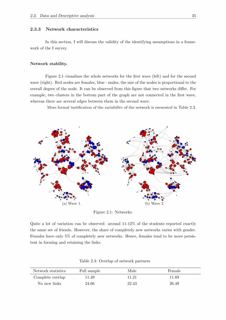
2.3. Data and Descriptive analysis 35
2.3.3 Network characteristics
In this section, I will discuss the validity of the identifying assumptions in a frame-
work of the I survey.
Network stability.
Figure 2.1 visualizes the whole networks for the first wave (left) and for the second
wave (right). Red nodes are females, blue - males, the size of the nodes is proportional to the
overall degree of the node. It can be observed from this figure that two networks differ. For
example, two clusters in the bottom part of the graph are not connected in the first wave,
whereas there are several edges between them in the second wave.
More formal justification of the variability of the network is presented in Table 2.3.
●
●
●
●
●
●
●
●●
●●
●
●●
●
●
●
●
● ●
●
●
●
●
●
●
●
●
●
●
●
●
●
●
●
●
●
●●
●
●
●
●
●●
●
●
●
●
●
●●
●
●
●
●
●
●
●
●
●
●
●
●
●
●
●
●
●
●
●
●
●
●
●
●
●
●
●
●
●
●
●
●
●
●
●
●
●
●
●
●●
● ●
●
●
●
●
●
●
●
●
●
●
●
●
●
●
●
●
●
●
●●
●
●
●
●
●
●
●●
●
●●
●
●
●
●
●
●
●
●
●
●
●
●
●
●●
●
●
●
●
●
●
●
●●
●
●
●
●
●
●
●
●
●
●
●
●
●
●
●
●
●
●
●
●
●
●
●
●
●
●
●
●
●
●
●
●
●
●
●
●
●
●
●
●
●
●●
●
●
●
●
● ●
●
●
●
●
●
●
●
●
●
●
●
●
●
●
●
●
●●
●
●
●
●
●
●
●
●
●
●
●
●
●
●
●
●
●
●
●
●
●
●
●
●
●●
●
●
● ●●
●
●
●
●
●
●
●
●
●
●
●
●●
●
●
●
(a) Wave 1.
●
●
●
●
●
●
●
●
●
●
●
●
●●
●
●
●
●
● ●
●
●
●
●
●
●
●
●
●
●
●
●
●
●
●
●
●
●●
●
●
●
●
●●
●
●
●
●●
●●
●
●
●
●
●
●
●
●●
●
●
●
●
●
●
●
●
●
●
●
●
●
●
●
●
●
●
●
●
●
●
●
●
●
●
●
●
●
●
●●
● ●
●
●
●
●
●
●
●
●
●
●
●
●
●
●
●
●
●
●
●●
●
●
●
●
●
●
●●
●
●●
●
●
●
●
●
●
●
●
●
●
●
●
●
●●
●
●
●
●
●
●
●
●●
●
●
●
●
●
●
●
●
●
●
●
●
●
●
●
●
●
●
●
●
●
●
●
●
●
●
●
●
●
●
●
●
●
●
●
●
●
●
●
●
●
● ●
●
●
●
●
● ●
●
●
●
●
●
●
●
●
●
●
●
●
●
●
●
●
●●
●
●
●
●
●
●
●
●
●
●
●
●
●
●
●
●
●
●
●
●
●
●
●
●
●●
●
●
●●
●
●
●
●
●
●
●
●
●
●
●
●
●●
●
●
●
(b) Wave 2.
Figure 2.1: Networks.
Quite a lot of variation can be observed: around 11-12% of the students reported exactly
the same set of friends. However, the share of completely new networks varies with gender.
Females have only 5% of completely new networks. Hence, females tend to be more persis-
tent in forming and retaining the links.
Table 2.3: Overlap of network partners
Network statistics Full sample Male Female
Complete overlap 11.49 11.21 11.89
No new links 24.66 22.43 26.49
36 Chapter 2. Endogenous Shocks in Social Networks
Partial overlap 65.20 46.73 77.30
Complete turnover 12.16 24.30 5.41
Observations 296 107 185
Note: Percentages of 1st, 3rd, and 4th rows do not add up to 100%, because there are new observations in
the 2nd wave, for which we do not observe the network in the 1st wave
Table 2.4 provides more evidence of the network variation: only around 16% of the links
survived after the first period, and around 78% of the links formed in the second period are
new.
Table 2.4: Some network characteristics
Network statistics Definition 1 year 2 year
Average indegree Average number of ingoing
ties
4.96 (2.73) 3.93 (2.53)
Average outdegree Average number of outgoing
ties
4.96 (2.01) 3.93 (2.2)
Density Proportion of existing ties in
the network
0.015 0.014
Reciprocity Proportion of ties which are
reciprocated
0.639 0.636
Transitivity The ratio of the triangles and
the connected triples in the
graph
0.454 0.443
Share of the links that remained from the 1st
wave in total amount of links of the 2nd wave
- 22.61%
Share of the links that remained from the 1st
wave in total amount of links of the 1st wave
16.57% -
Transitivity
. Table 2.4 describes several characteristics of the networks in the sample. The tran-
sitivity is measured by the shares total amount of connected triangles in the whole graph.
So in more than 50% of all possible sets of three students, at least, one link is missing.
Figure2.2 shows the subgraph of the network to demonstrate the existence of intran-
sitive triads in both of the samples. For example, in wave 1 the following triad is intransitive:
717 → 694, 694 → 779, but 717 9 779. Other examples of intransitive triads are: 939→693→ 778, 693→778→ 878 in the first wave and 939→ 779→ 694, 779→ 694→ 717 in the
second wave, and some more.
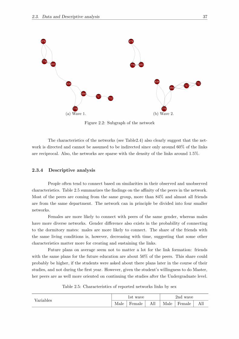
2.3. Data and Descriptive analysis 37
732717
878
778693
939
694
779
(a) Wave 1.
732717
878
778 693
939
694
779
(b) Wave 2.
Figure 2.2: Subgraph of the network
The characteristics of the networks (see Table2.4) also clearly suggest that the net-
work is directed and cannot be assumed to be indirected since only around 60% of the links
are reciprocal. Also, the networks are sparse with the density of the links around 1.5%.
2.3.4 Descriptive analysis
People often tend to connect based on similarities in their observed and unobserved
characteristics. Table 2.5 summarizes the findings on the affinity of the peers in the network.
Most of the peers are coming from the same group, more than 84% and almost all friends
are from the same department. The network can in principle be divided into four smaller
networks.
Females are more likely to connect with peers of the same gender, whereas males
have more diverse networks. Gender difference also exists in the probability of connecting
to the dormitory mates: males are more likely to connect. The share of the friends with
the same living conditions is, however, decreasing with time, suggesting that some other
characteristics matter more for creating and sustaining the links.
Future plans on average seem not to matter a lot for the link formation: friends
with the same plans for the future education are about 50% of the peers. This share could
probably be higher, if the students were asked about there plans later in the course of their
studies, and not during the first year. However, given the student’s willingness to do Master,
her peers are as well more oriented on continuing the studies after the Undergraduate level.
Table 2.5: Characteristics of reported networks links by sex
Variables1st wave 2nd wave
Male Female All Male Female All
38 Chapter 2. Endogenous Shocks in Social Networks
Average size 4.53 5.19 4.96 3.57* 4.18* 3.93*
Average size (with out of sample links) 5.22 5.78 5.58 4.29* 4.96* 4.69*
Study group/department relation (% of network partners)
Same group 84.17 87.23 86.76 87.21 89.89 88.78
Same department 98.54 99.21 98.99 97.54 99.39 98.95
Individual characteristics of network partners(% of network partners)
Same gender 64.05 81.97 76.18
Same working status 62.43 70.33 67.78 50.74 60.95 56.41
Same education of mother 61.75 66.84 65.19 - - -
Same education of father 56.45 50.08 52.14 - - -
Same living conditions 57.59 46.71 50.23 50.97 39.61 43.33
Same living conditions (dorm/not) 84.14 76.23 78.79 74.27 70.55 72.16
Future plans (% of network partners)
Same plans for Master 54.44 57.37 56.41 - - -
Same plans for Doctorate 47.18 47.32 47.27 - - -
Subsample of planning to do Master:
Same plans for Master 68.34 72.42 74.46 - - -
*the network data in the 2nd wave is truncated at 7 friends
More than 1/3 of all links in the first wave are links to the students with retakes
(37%). The share of the links to the students with retakes in the first period in the total
amount of second wave links is slightly smaller: 33%. It might be caused by the intention
of students to improve their peer group and connect to peers with higher outcomes. The
average amount of the friends with retakes in the first period is 1.83 while it is lower for the
second period: only 1.25. The average amount of peers with exam retakes for the subsample
of all students that have at least one peer with retake is higher than the average of the
full sample and is equal to 2.5. For the same students in the second wave, the average
number of peers who had exam retakes in the first period is now much lower: 1.55. It can be
suspected that the decrease in this value may be partially explained by the readjustments
of the network towards better connections. Moreover, for the same subsample, the average
number of peers with retakes in the second period is even lower: 1.37. Interestingly, some of
those, who didn’t have any friends with retakes in the first period, connected to new peers
that had the retakes in the second period, the average number of such friends is only 0.35
though, but the average number of friends with retakes in the next period is 0.57. So the
changes in the network are leading to the improvements as well as worsening of the new peer
group. These findings are summarized in the Table 2.6.
Table 2.6: Distribution of retakes
Links wave 1,
retakes wave 1
Links wave 2,
retakes wave 1
Links wave 2,
retakes wave 2
Share of retakes links in all links 36.99% 32.99% 29.15%
Average amount of friends with retakes 1.83 1.25 1.15
Subsample with retakes of friends2.5 1.55 1.37
2.4. Results 39
Average amount of friends with retakes
Subsample no retakes of friends0 0.35 0.57
Average amount of friends with retakes
Observe that students in the studied framework tend to connect to peers, having
higher average grades than the students themselves, for the full sample as well as for the
samples with and without retake friends. Students, who do not connect to peers with re-
takes, are performing better than those, whose friends are having retakes. However, the
improvements in the performance in the future are not significant, with the changes in the
performance of the students without peers’ retakes being slightly higher.
Table 2.7: Average grades in samples and subsamples
Full sample With retakes of friends No retakes of friends
Average grade7.04 6.98 7.37
(0.99) (0.96) (0.98)
Average grade of friends7.18 7.03 7.68
(0.65) (0.63) (0.49)
Sample size 320 234 86
Average grade next period7.13 7.02 7.44
(1.14) (1.15) (1.07)
Sample size 297 217 80
It is not possible to distinguish between the predicted and unexpected components of
retakes by simply looking at the data. Therefore, the deeper econometric analysis is needed
to make conclusions about the existence and the magnitude of the effect of unpredicted
shock.
2.4 Results
2.4.1 Main specification
I use the following variables for the main specification of the model:
Outcome: average weighted grade of the student in the corresponding period. The grades
are summed up weighted by the amount of the credits assigned to the particular course.
Retakes: indicator of at least one retake in the first period.
Initial ability, measured as the sum of mandatory Unified State Examinations (mathe-
matics and Russian) plus the sum of cross-products between these USE results and a
dummy of winning any relevant Olympiads.
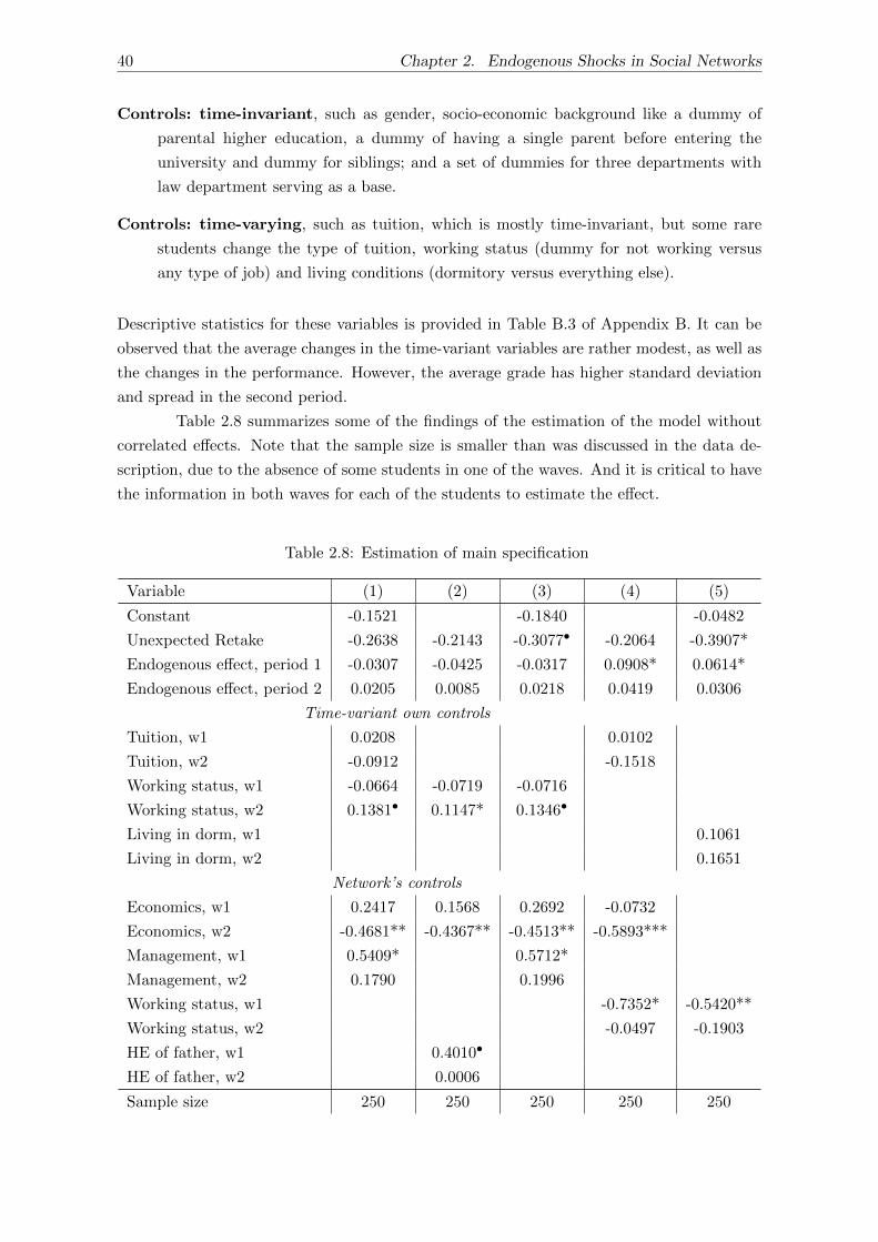
40 Chapter 2. Endogenous Shocks in Social Networks
Controls: time-invariant, such as gender, socio-economic background like a dummy of
parental higher education, a dummy of having a single parent before entering the
university and dummy for siblings; and a set of dummies for three departments with
law department serving as a base.
Controls: time-varying, such as tuition, which is mostly time-invariant, but some rare
students change the type of tuition, working status (dummy for not working versus
any type of job) and living conditions (dormitory versus everything else).
Descriptive statistics for these variables is provided in Table B.3 of Appendix B. It can be
observed that the average changes in the time-variant variables are rather modest, as well as
the changes in the performance. However, the average grade has higher standard deviation
and spread in the second period.
Table 2.8 summarizes some of the findings of the estimation of the model without
correlated effects. Note that the sample size is smaller than was discussed in the data de-
scription, due to the absence of some students in one of the waves. And it is critical to have
the information in both waves for each of the students to estimate the effect.
Table 2.8: Estimation of main specification
Variable (1) (2) (3) (4) (5)
Constant -0.1521 -0.1840 -0.0482
Unexpected Retake -0.2638 -0.2143 -0.3077• -0.2064 -0.3907*
Endogenous effect, period 1 -0.0307 -0.0425 -0.0317 0.0908* 0.0614*
Endogenous effect, period 2 0.0205 0.0085 0.0218 0.0419 0.0306
Time-variant own controls
Tuition, w1 0.0208 0.0102
Tuition, w2 -0.0912 -0.1518
Working status, w1 -0.0664 -0.0719 -0.0716
Working status, w2 0.1381• 0.1147* 0.1346•
Living in dorm, w1 0.1061
Living in dorm, w2 0.1651
Network’s controls
Economics, w1 0.2417 0.1568 0.2692 -0.0732
Economics, w2 -0.4681** -0.4367** -0.4513** -0.5893***
Management, w1 0.5409* 0.5712*
Management, w2 0.1790 0.1996
Working status, w1 -0.7352* -0.5420**
Working status, w2 -0.0497 -0.1903
HE of father, w1 0.4010•
HE of father, w2 0.0006
Sample size 250 250 250 250 250

2.4. Results 41
BIC -216.68 -225.24 -226.51 -225.79 -196.71
*** - p-value < 0.01, ** - p-value < 0.05, * - p-value < 0.1, • - p-value < 0.15
It can be observed that for the full sample the estimator of the effect of the unpre-
dicted component of retakes is negative but in most cases insignificant. The magnitude of
the effect in specification (5) suggests that if a friend of some student had a retake during
the first year, which this student couldn’t predict at all, the difference between the average
grade of year 2 and the average grade of year 1 of the student will be on average 0.05-0.39
lower, than in the case the student expected the retake of a friend, depending on the total
number of friends. For example, the median student on average improves her grades in the
second period in comparison to the first by 0.24, which is 2.4% of the maximum grade. The
presence of unpredicted retake of the friend, other things equal, may leave the average grade
in the second period at the same level or even decrease it up to 1.5% of maximum grade,
changing the direction of the dynamics and, moreover, putting the student on average 5-25
positions lower in the overall students’ rating, falling lower with less friends.
Note, that there is a highly significant difference between the economics and other
departments for most of the specifications. On average, students of economics department
have -0.5 lower difference of grades, which suggest the overall lower grades of the economics
department in the second year. This evidence indicates the necessity of using the model with
correlated effects or treating the departments separately by splitting the full sample.
Discussing the results for those, who had their own retakes, versus those, who did
not is the other possible way to improve the estimation results.
The further analysis is given in the next subsections, where I present the results of
estimation in the subsamples, of the model with correlated effects, as well as the estimation
with a possibly improved network. However, it is worth pointing out, that the sample size
for the main specification is 250 students, which may be not sufficiently big to capture the
desired effect, and the results of the estimation in the subsamples should be treated with
even more care, since with the lower sample size the asymptotic properties of the proposed
estimator may suffer.
2.4.2 Connection to one’s own retake
I first report the results for the subsamples of students with and without own retakes.
It can be suggested that the students that had their own retake may, in general, be connected
to worse peers. Therefore, having friends with retakes might lower the performance even
further, whereas the friends’ retakes are more likely to have either no effect or even positive
influence for the better students.
Table 2.9: Presence of own retake
Variable (1), yes (2), yes (1), no (2), no
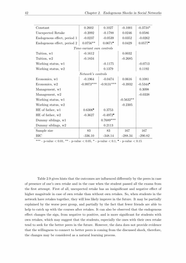
42 Chapter 2. Endogenous Shocks in Social Networks
Constant 0.2602 0.1027 -0.1001 -0.3734*
Unexpected Retake -0.2092 -0.1788 0.0246 0.0586
Endogenous effect, period 1 -0.0237 -0.0539 0.0352 -0.0262
Endogenous effect, period 2 0.0756** 0.0671• 0.0429 0.0577•
Time-variant own controls
Tuition, w1 -0.1612 0.0032
Tuition, w2 -0.1834 -0.2685
Working status, w1 -0.1175 -0.0713
Working status, w2 0.1379 0.1192
Network’s controls
Economics, w1 -0.1964 -0.0474 0.0616 0.1081
Economics, w2 -0.9973*** -0.9131*** -0.3932 -0.5344•
Management, w1 0.3098
Management, w2 -0.0338
Working status, w1 -0.5632**
Working status, w2 -0.2305
HE of father, w1 0.6306• 0.3753
HE of father, w2 -0.3627 -0.4972•
Dummy siblings, w1 0.7689***
Dummy siblings, w2 0.2113
Sample size 83 83 167 167
BIC -336.10 -348.14 -288.34 -290.82
*** - p-value < 0.01, ** - p-value < 0.05, * - p-value < 0.1, • - p-value < 0.15
Table 2.9 gives hints that the outcomes are influenced differently by the peers in case
of presence of one’s own retake and in the case when the student passed all the exams from
the first attempt. First of all, unexpected retake has an insignificant and negative effect of
higher magnitude in case of own retake than without own retakes. So, when students in the
network have retakes together, they will less likely improve in the future. It may be partially
explained by the worse peer group, and partially by the fact that fewer friends are able to
help to catch up with the courses after retakes. It can also be observed that the endogenous
effect changes the sign, from negative to positive, and is more significant for students with
own retakes, which may suggest that the students, especially the ones with their own retake
tend to seek for the better peers in the future. However, the data does not provide evidence
that the willingness to connect to better peers is coming from the discussed shock, therefore,
the changes may be considered as a natural learning process.
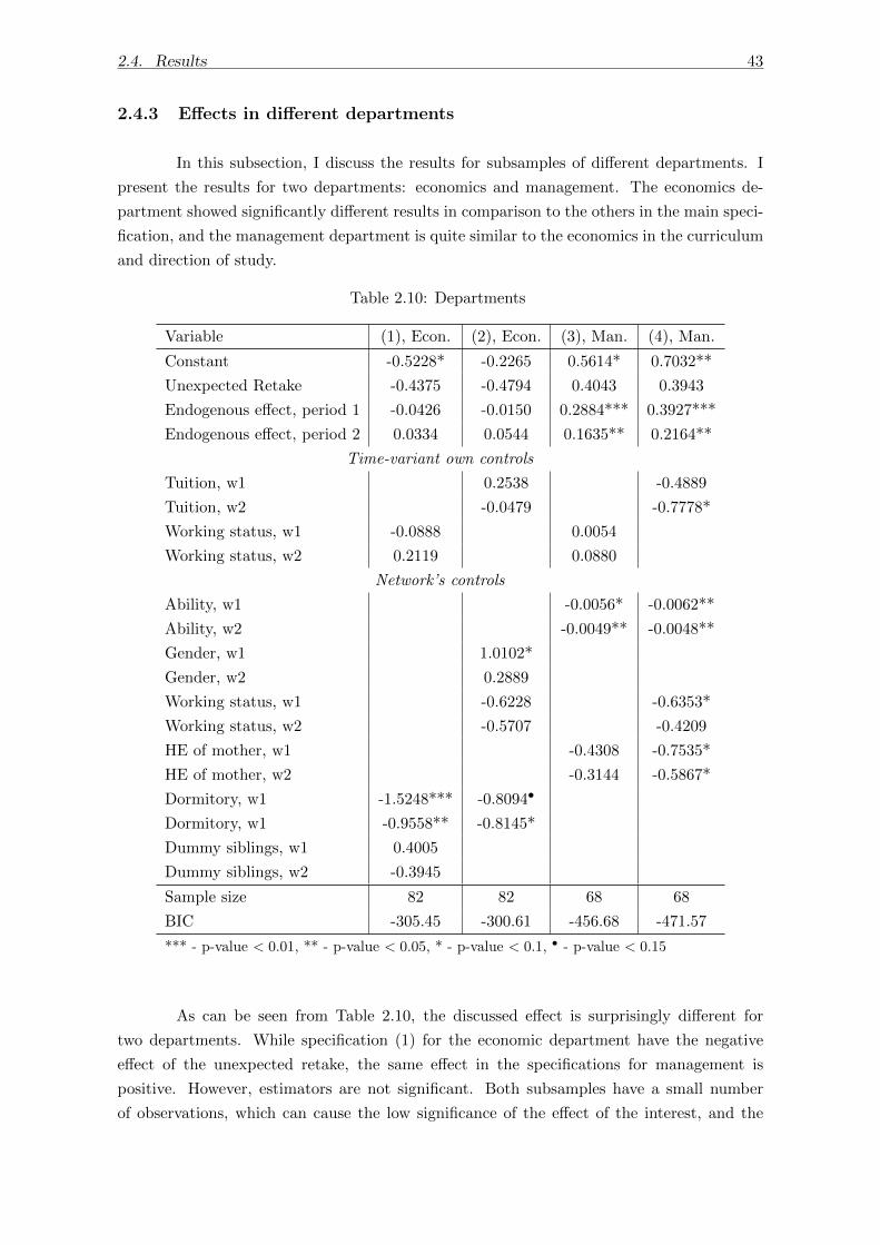
2.4. Results 43
2.4.3 Effects in different departments
In this subsection, I discuss the results for subsamples of different departments. I
present the results for two departments: economics and management. The economics de-
partment showed significantly different results in comparison to the others in the main speci-
fication, and the management department is quite similar to the economics in the curriculum
and direction of study.
Table 2.10: Departments
Variable (1), Econ. (2), Econ. (3), Man. (4), Man.
Constant -0.5228* -0.2265 0.5614* 0.7032**
Unexpected Retake -0.4375 -0.4794 0.4043 0.3943
Endogenous effect, period 1 -0.0426 -0.0150 0.2884*** 0.3927***
Endogenous effect, period 2 0.0334 0.0544 0.1635** 0.2164**
Time-variant own controls
Tuition, w1 0.2538 -0.4889
Tuition, w2 -0.0479 -0.7778*
Working status, w1 -0.0888 0.0054
Working status, w2 0.2119 0.0880
Network’s controls
Ability, w1 -0.0056* -0.0062**
Ability, w2 -0.0049** -0.0048**
Gender, w1 1.0102*
Gender, w2 0.2889
Working status, w1 -0.6228 -0.6353*
Working status, w2 -0.5707 -0.4209
HE of mother, w1 -0.4308 -0.7535*
HE of mother, w2 -0.3144 -0.5867*
Dormitory, w1 -1.5248*** -0.8094•
Dormitory, w1 -0.9558** -0.8145*
Dummy siblings, w1 0.4005
Dummy siblings, w2 -0.3945
Sample size 82 82 68 68
BIC -305.45 -300.61 -456.68 -471.57
*** - p-value < 0.01, ** - p-value < 0.05, * - p-value < 0.1, • - p-value < 0.15
As can be seen from Table 2.10, the discussed effect is surprisingly different for
two departments. While specification (1) for the economic department have the negative
effect of the unexpected retake, the same effect in the specifications for management is
positive. However, estimators are not significant. Both subsamples have a small number
of observations, which can cause the low significance of the effect of the interest, and the
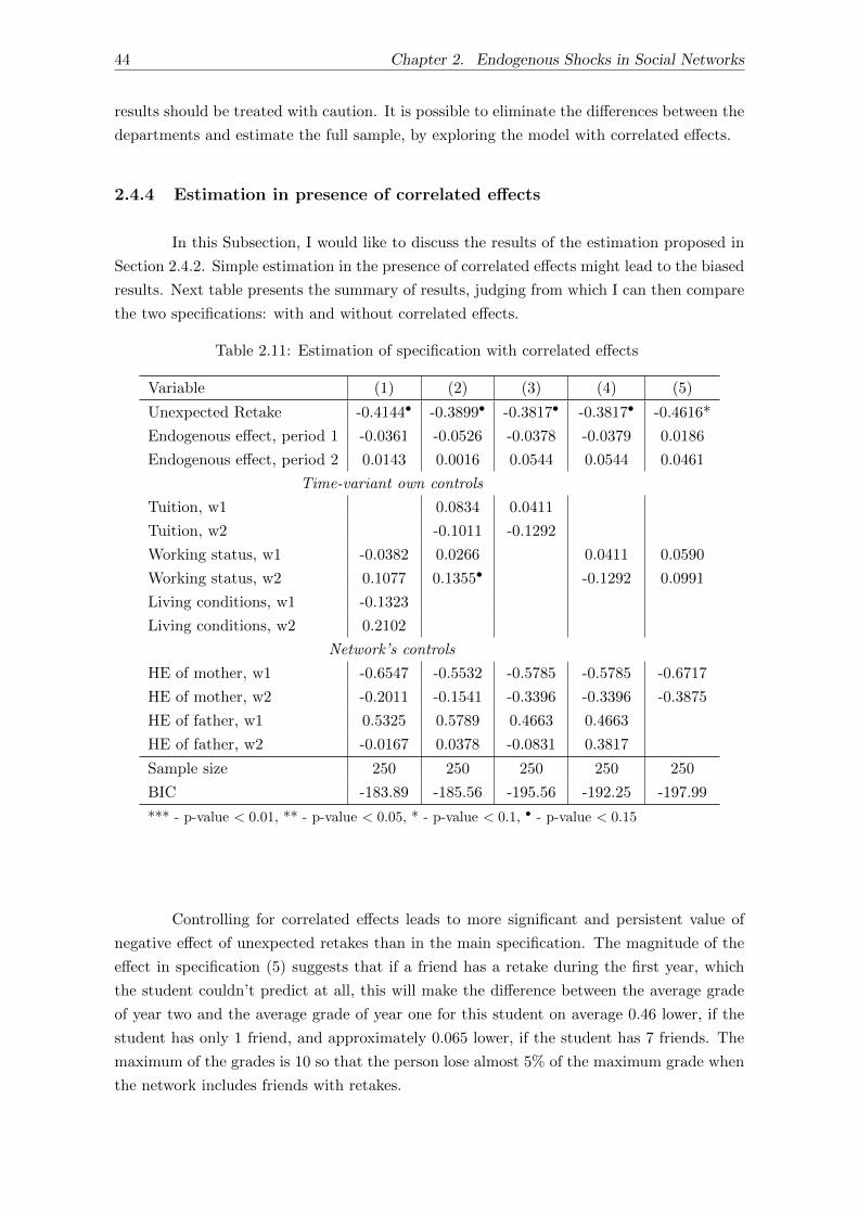
44 Chapter 2. Endogenous Shocks in Social Networks
results should be treated with caution. It is possible to eliminate the differences between the
departments and estimate the full sample, by exploring the model with correlated effects.
2.4.4 Estimation in presence of correlated effects
In this Subsection, I would like to discuss the results of the estimation proposed in
Section 2.4.2. Simple estimation in the presence of correlated effects might lead to the biased
results. Next table presents the summary of results, judging from which I can then compare
the two specifications: with and without correlated effects.
Table 2.11: Estimation of specification with correlated effects
Variable (1) (2) (3) (4) (5)
Unexpected Retake -0.4144• -0.3899• -0.3817• -0.3817• -0.4616*
Endogenous effect, period 1 -0.0361 -0.0526 -0.0378 -0.0379 0.0186
Endogenous effect, period 2 0.0143 0.0016 0.0544 0.0544 0.0461
Time-variant own controls
Tuition, w1 0.0834 0.0411
Tuition, w2 -0.1011 -0.1292
Working status, w1 -0.0382 0.0266 0.0411 0.0590
Working status, w2 0.1077 0.1355• -0.1292 0.0991
Living conditions, w1 -0.1323
Living conditions, w2 0.2102
Network’s controls
HE of mother, w1 -0.6547 -0.5532 -0.5785 -0.5785 -0.6717
HE of mother, w2 -0.2011 -0.1541 -0.3396 -0.3396 -0.3875
HE of father, w1 0.5325 0.5789 0.4663 0.4663
HE of father, w2 -0.0167 0.0378 -0.0831 0.3817
Sample size 250 250 250 250 250
BIC -183.89 -185.56 -195.56 -192.25 -197.99
*** - p-value < 0.01, ** - p-value < 0.05, * - p-value < 0.1, • - p-value < 0.15
Controlling for correlated effects leads to more significant and persistent value of
negative effect of unexpected retakes than in the main specification. The magnitude of the
effect in specification (5) suggests that if a friend has a retake during the first year, which
the student couldn’t predict at all, this will make the difference between the average grade
of year two and the average grade of year one for this student on average 0.46 lower, if the
student has only 1 friend, and approximately 0.065 lower, if the student has 7 friends. The
maximum of the grades is 10 so that the person lose almost 5% of the maximum grade when
the network includes friends with retakes.
2.4. Results 45
2.4.5 Additional analysis
Improving network
As it was mentioned before, students were asked to name up to 7 friends from their
cohort, although some named more than 7. However, it is reasonable to assume that all
named friends are not equal for the person. I introduce two possible ways to account for
better friends so that the quality of the network can be improved.
First, I assume that the friends named among the first are more important than
the others, since they were remembered earlier, and the best friends can’t be named last.
I reduced the network, only taking up to three named first students. I conducted analysis
for both models with and without accounting for correlated effects. The suggested improve-
ment of the network didn’t, however, increased the significance of the results12. The effect
of an unpredicted component of friends’ exam retake is not significantly different from zero.
Therefore, it might be reasonable to conclude that the unexpected negative or positive per-
formance of the whole network of friends is more important for the future performance of
students than the performance of only best friends.
Second, I observe that about 60% of the network is reciprocal, so I conduct similar
analysis limiting the network to only reciprocal connections. This again does not bring any
improvement in terms of the significance of the studied effect. It seems that the students’
performance is shaped not only by their mutual friends, but although by those, who don’t
consider them as friends, but are considered as friends by the students. These students may
be viewed as a sort of role models, and therefore, are important to be taken into account.
Thus, the initial full network is able to capture the effect of unexpected shock better
than the versions of the network, considered initially as possible improvements.
Important classes
The further analysis divides the subjects, studied by the students in the sample, into
two parts: more important and less important. All subjects have the corresponding amount
of ECTS credits, from 0 to 8 with average around 2.5. For the analysis, I set the threshold
of 4 ECTS points. However, some subjects have several exams, for example, Mathematical
Analysis, and the weight of some of the exam in the series can be lower than 4, but, at least,
one exam has ECTS higher than 4. In these cases, I am including all the exams of the series
in the sample of important exams. This restricts the set of the students with retakes to 2/3
of the initial set.
Table 2.12 provides the results of the analysis in the new setting for the model
without correlated effects.
Table 2.12: Estimation with retakes for classes with ECTS 4 and higher
12The detailed results are presented in Tables B.4, B.5 in Appendix B
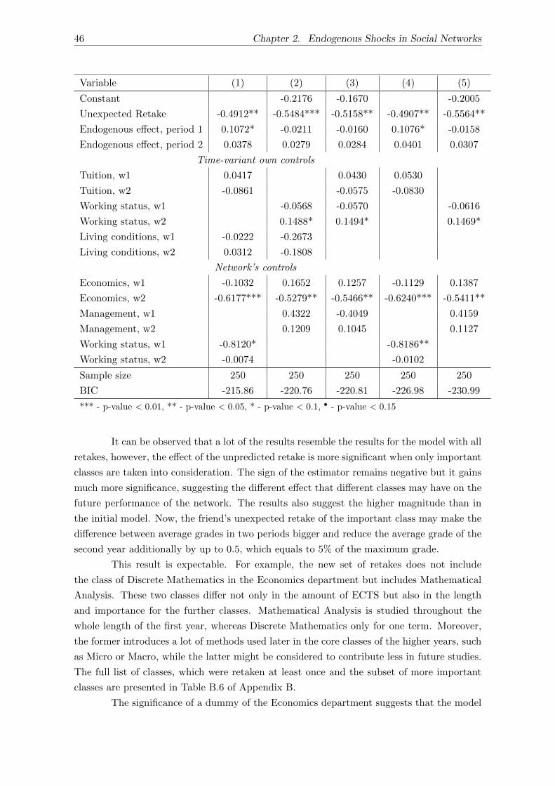
46 Chapter 2. Endogenous Shocks in Social Networks
Variable (1) (2) (3) (4) (5)
Constant -0.2176 -0.1670 -0.2005
Unexpected Retake -0.4912** -0.5484*** -0.5158** -0.4907** -0.5564**
Endogenous effect, period 1 0.1072* -0.0211 -0.0160 0.1076* -0.0158
Endogenous effect, period 2 0.0378 0.0279 0.0284 0.0401 0.0307
Time-variant own controls
Tuition, w1 0.0417 0.0430 0.0530
Tuition, w2 -0.0861 -0.0575 -0.0830
Working status, w1 -0.0568 -0.0570 -0.0616
Working status, w2 0.1488* 0.1494* 0.1469*
Living conditions, w1 -0.0222 -0.2673
Living conditions, w2 0.0312 -0.1808
Network’s controls
Economics, w1 -0.1032 0.1652 0.1257 -0.1129 0.1387
Economics, w2 -0.6177*** -0.5279** -0.5466** -0.6240*** -0.5411**
Management, w1 0.4322 -0.4049 0.4159
Management, w2 0.1209 0.1045 0.1127
Working status, w1 -0.8120* -0.8186**
Working status, w2 -0.0074 -0.0102
Sample size 250 250 250 250 250
BIC -215.86 -220.76 -220.81 -226.98 -230.99
*** - p-value < 0.01, ** - p-value < 0.05, * - p-value < 0.1, • - p-value < 0.15
It can be observed that a lot of the results resemble the results for the model with all
retakes, however, the effect of the unpredicted retake is more significant when only important
classes are taken into consideration. The sign of the estimator remains negative but it gains
much more significance, suggesting the different effect that different classes may have on the
future performance of the network. The results also suggest the higher magnitude than in
the initial model. Now, the friend’s unexpected retake of the important class may make the
difference between average grades in two periods bigger and reduce the average grade of the
second year additionally by up to 0.5, which equals to 5% of the maximum grade.
This result is expectable. For example, the new set of retakes does not include
the class of Discrete Mathematics in the Economics department but includes Mathematical
Analysis. These two classes differ not only in the amount of ECTS but also in the length
and importance for the further classes. Mathematical Analysis is studied throughout the
whole length of the first year, whereas Discrete Mathematics only for one term. Moreover,
the former introduces a lot of methods used later in the core classes of the higher years, such
as Micro or Macro, while the latter might be considered to contribute less in future studies.
The full list of classes, which were retaken at least once and the subset of more important
classes are presented in Table B.6 of Appendix B.
The significance of a dummy of the Economics department suggests that the model
2.5. Conclusion 47
with correlated effects may be used, as in the model with the full set of retakes. Surprisingly,
the estimator of the effect of the unexpected retake in the model with correlated effects loses
the significance once I restrict the set of the retakes.
2.5 Conclusion
The paper discusses the spread of the unpredicted shock across the network of friends
in the university environment using the newly introduced dynamic peer effect model in the
presence of endogenous shock.
Exam retakes play an important role in determining the future of the student. How-
ever, it was shown that the unpredicted component of the retake may influence not only the
students with a retake but also the whole network of friends. In most of the cases the effect
is not very significant, but still should not be ignored. When the threshold of failing the
exam is too high, some students, viewed by their friends as high-achievers, are likely to fail.
This anticipation mistake leads to the decrease of the average grades of the whole friendship
network.
The ideas explored in this paper can be further extended to the analysis of the net-
works in other settings, not only for educational outcomes. The method is applicable, when
the endogenous shocks might have the longitudinal effect on the network outcomes, such
as, for example, a treatment that for some reasons cannot be randomized, or conversational
networks in developing communities, etc.
I have presented the results for identification of such models, that allow disentan-
gling the effect of unpredicted shock on the future performance. The findings of the paper
suggest that it is sufficient to assume time-variability of networks together with the exis-
tence of intransitive triads (or distances of length three, depending on the correlated effects
assumption) in each of the states of the network for the similar models. Intransitive triads
are guaranteed by the presence of two students only connected via the third common friend
but not directly. The characteristics of friends of the friends don’t influence directly the
outcome, and, therefore, can be used as an instrumental variable for the friends’ outcome.
Such instruments can, therefore, deal with endogeneity issue. The group of new friends,
different from the group of old friends, let the model capture the changes, happening due to
the shock.
The procedure developed in the paper is shown to yield consistent estimators of the
individual characteristics, endogenous peer effect and effect of unpredicted shock.
All theoretical findings are tested on the dataset of university students, connected
via the friendship network. Most of the empirical evidence suggest that the unpredicted
exam retakes of the friends will have a negative effect on the changes of the performance
of students. This effect is more prominent for students with own retakes and for students
in the Economics department. The higher significance of the estimators in the model with
correlated effects gives evidence of the presence of unobserved homophily that influences
link formation. Change of sign of endogenous effect for students with own retakes shows the

48 Chapter 2. Endogenous Shocks in Social Networks
importance of further exploration of the problem and improvement of the model by inclusion
of the link formation mechanism.
Appendix 49
Appendix
A. Main proofs
Regularity conditions (adaptation of L. Lee (2003)):
Assumption 1. The matrices (I − β1G1) and (I − β2G2) are nonsingular
Assumption 2. The row and column sums of the matrices G1, G2, (I − β1G1)−1 and(I − β2G2)−1 are uniformly bounded in absolute value.
Assumption 3. The elements of the matrices X1 and X2 are uniformly bounded in absolutevalue
Assumption 4. The error terms {νi : 1 ≤ i ≤ n} are identically distributed. Furthermore,they are distributed (jointly) independently with E[νiX
1i ] = 0 and E[ν2i ] = σν < ∞.
Additionally, they are assumed to possess finite fourth moments. The error terms{∆εi : 1 ≤ i ≤ n} are identically distributed. Furthermore, they are distributed(jointly) independently with E[∆εi] = 0 and E[∆ε2i ] = σε1 + σε2 < ∞. Additionally,they are assumed to possess finite fourth moments
Assumption 5. The limit J = limn→∞1nZ
TZ exists and is nonsingular.
Assumption 6. The limit J = limn→∞1nZ
TZ exists and is nonsingular.
Assumption 7. Step 1. The initial estimator β12SLS of β1 is na-consistent for some a > 0.The initial estimators α1
2SLS , γ12SLS and δ12SLS are consistent estimators of α1, γ1 andδ1, respectively. Step 2. The initial estimators β1,2SLS and β2,2SLS of β1 and β2 arenb-consistent for some b > 0. The initial estimators α1,2SLS , α2,2SLS , γ1,2SLS , γ2,2SLS ,δ1,2SLS and δ2,2SLS are consistent estimators of α1, α2, γ1, γ2, δ1 and δ2, respectively.
Proof of Lemma 1.
The structural form equation:
P (retakei) = α1 + β1∑j 6=i
G1ijy
1j + γ1X1
i + δ1∑j 6=i
G1ijX
1j + νi, E[νi|X] = 0
can be rewritten in the reduced form in the following manner:
PR = α1i+ β1G1y1 + γ1X1 + δ1G1X1 + ν, E[ν|X1] = 0
PR = α1i+ β1G1y1 + (γ1I + δ1G1)X1 + ν, E[ν|X1] = 0
Taking conditional expectations:
E[PR|X1] = α1i+ β1G1E[y1|X1] + (γ1I + δ1G1)X1
Note that y can be expressed in terms of peer effect model as the one used for the probabilityof retakes:
y1i = α0 + β0∑j 6=i
G1ijy
1j + γ0X
1i + δ0
∑j 6=i
G1ijX
1j + ξi, E[ξi|X] = 0
50 Chapter 2. Endogenous Shocks in Social Networks
with reduced form:
y1 = α0i+ β0G1y1 + (γ0I + δ0G
1)X1 + ξ, E[ξ|X] = 0
Then following steps of Bramoulle, Djebbari, and Fortin (2009):
y1 = α0(I − β0G1)−1 + (I − β0G1)−1(γ0I + δ0G1)X1 + (I − β0G1)−1ξ, E[ξ|X] = 0
Using (I − β0G1)−1 =∑∞
k=0 βk0(G1)
k:
y1 = α0(I − β0G1)−1 + γ0X1 + (γ0β0 + δ0)
∞∑k=0
βk0(G1)k+1X1 +
∞∑k=0
βk0(G1)kξ
And the expected mean friends’ groups’ performance conditional on X1 can be written as:
E[G1y1|X1] = α0(I − β0G1)−1 + γ0G1X1 + (γ0β0 + δ0)
∞∑k=0
βk0(G1)k+2X1
As was proven in Bramoulle, Djebbari, and Fortin (2009), if γ0β0 + δ0 6= 0 and I,G1 and(G1)2 are linearly independent, the social effects are identified. So this expression can beplugged-in into the reduced form of the equation for the probability of retake.
E[PR|X1] = α1i+ β1(α0(I − β0G1)−1 + γ0G1X1 + (γ0β0 + δ0)
∞∑k=0
βk0(G1)k+2X1) +
+(γ1I + δ1G1)X1 = (α1I + β1α0(I − β0G1)−1)) +
+β1(γ0β0 + δ0)
∞∑k=0
βk0(G1)k+2X1 + (γ1I + (β1γ0 + δ1)G1)X1
or
E[PR|X1] = α1I+β1(α0(I−β0G1)−1+β1(I−β0G1)−1(γ0I+δ0G1)G1X1+(γ1I+δ1G1)X1
Now consider two sets of structural parameters (α1, β1, γ1, δ1) and (α1, β1, γ1, δ1)leading to the same reduced form. It means that:
α1I + β1α0(I − β0G1)−1 = α1I + β1α0(I − β0G1)−1
α1I − α1β0G1 + β1α0I = α1I − α1β0G
1 + β1α0I
(α1 − α1)I + (β1α0 − β1α0)I − (α1β0 − α1β0)G1 = 0
(α1 − α1 + (β1 − β1)α0)I = (α1 − α1)β0G1
and:
β1(I−β0G1)−1(γ0I+δ0G1)G1+(γ1I+δ1G1) = β1(I−β0G1)−1(γ0I+δ0G
1)G1+(γ1I+δ1G1)
β1(γ0I+δ0G1)G1+(I−β0G1)(γ1I+δ1G1) = β1(γ0I+δ0G
1)G1+(I−β0G1)(γ1I+ δ1G1)
β1γ0G1 + β1δ0(G
1)2 + (γ1I − (β0γ1 − δ1)G1)− β0δ1(G1)
2) = β1γ0G
1 + β1δ0(G12) +
+(γ1I − (β0γ1 − δ1)G1)− β0δ1(G1)
2)
γ1I+(β1γ0+β1δ0−β0γ1+δ1)G1−β0δ1(G1)2
= γ1I+(β1γ0+β1δ0−β0γ1+δ1)G1−β0δ1(G1)2
Appendix 51
(γ1 − γ1)I + ((β1 − β1)γ0 + (β1 − β1)δ0 − β0(γ1 − γ1) + δ1 − δ1)G1 + β0(δ1 − δ1)(G1)
2= 0
Now let I,G1 and (G1)2 be linearly independent. Then the above equality holds only if allthree coefficients are 0:
γ1 − γ1 = 0
(β1 − β1)γ0 + (β1 − β1)δ0 − β0(γ1 − γ1) + δ1 − δ1 = 0
β0(δ1 − δ1) = 0
If β0 6= 0 and γ20 +δ20 6= 0, two sets of coefficients (α1, β1, γ1, δ1) and (α1, β1, γ1, δ1) are equiv-alent. Note that the restrictions on the coefficients of the peer effect model suggest that themodel has an endogenous peer effect and the performance depends on own set of observedcharacteristics, or on peers observed characteristics, or on both. These requirements arenatural for the peer effect model and therefore, the identification result is achieved. �
Proof of Lemma 2. (Identification, Step 2, no correlated effects)
Recall the second step equation:
∆yi = (α2 − α1) + β2∑j 6=i
G2ijy
2j − β1
∑j 6=i
G1ijy
1j + δURi + γ2X
2i − γ1X1
i +
+δ2∑j 6=i
G2ijX
2j − δ1
∑j 6=i
G1ijX
1j + ∆εi
It can be rewritten in the reduced form as following:
∆y = (α2 − α1)i+ β2G2y2 − β1G1y1 + δUR+ γ2X
2TV − γ1X
1TV + δ2G
2X2−
−δ1G1X1 + ∆ε, with UR defined as discussed in Section 2 and E[∆ε] = 0
This can be further modified in the following manner:
E[∆y|X2] = (α2 − α1)i+ β2G2E[y2|X2]− β1G1E[y1|X2] + δE[UR|X2]+
+γ2X2TV − γ1X
1TV + δ2G
2X2 − δ1G1X1
with
E[y1|X2] = (I − β0,1G1)−1α0,1 + (I − β0,1G1)−1(γ0,1I + δ0,1G1)E[X1|X2] =
= (I − β0,1G1)−1α0,1 + (I − β0,1G1)−1(γ0,1I + δ0,1G1)X1,
since X1 is already known by the time X2 is revealed, therefore, the latter cannot add anynew information.
Also:
E[y2|X2] = (I − β0,2G2)−1α0,2 + (I − β0,2G2)−1(γ0,2I + δ0,2G2)X2
Note that UR is also defined at the first period, hence, the new information in X2 will notanything new for the expected value of the UR, hence E[UR|X2] = UR.
Also notice than in principle coefficients in the model in differences α1, β1, γ1, δ1,α2, β2, γ2, δ2 can be different from the corresponding coefficients in the single period peer
52 Chapter 2. Endogenous Shocks in Social Networks
effect models α0,1, β0,1, γ0,1, δ0,1, α0,2, β0,2, γ0,2, δ0,2. This can be due to the unaccounted insingle period model fixed effects that can be eliminated in the model in differences and dueto the presence of the shock in the model, which can take some of the effect, that would beotherwise attributed towards endogenous or exogenous effect.
Then, letting α = α2 − α1
E[∆y|X2] = αi+β2G2(I−β0,2G2)−1(α0,2+(γ0,2I+δ0,2G
2)X2)−β1G1(I−β0,1G1)−1(α0,1+
(γ0,1I + δ0,1G1)X1) + δUR+ γ2X
2TV − γ1X
1TV + δ2G
2X2 − δ1G1X1
First, if G1 = G1, then δ2 and δ1 are identified only partially, for time-variant vari-ables of X1 and X2 respectively. This assumption can be relaxed, if we let the coefficients ofthe single period coincide with the coefficients of the coefficients of the model in differences.Then, however, the following assumption need to be made δ = 0, meaning that the shockhas no effect on the outcome, which is not true in the setting of the model of the paper.Hence, G1 = G1 is one of the identifying assumptions for the second step model.
Next, I follow similar steps to the proof of Lemma 1. Consider two sets of the pa-rameters leading to the same reduced form, (α1, β1, γ1, δ1, α2, β2, γ2, δ2, δ) and (α1, β1, γ1, δ1,
α2, β2, γ2, δ2,˜δ). I do not include the single-period parameters, since their identification
is achieved separately, if I,G1, (G1)2 are linearly independent and if I,G2, (G2)2 are alsolinearly independent. Then:
αI + β2G2(I − β0,2G2)−1α0,2 − β1G1(I − β0,1G1)−1α0,1 =
= αI + β2G2(I − β0,2G2)−1α0,2 − β1G1(I − β0,1G1)−1α0,1
β2G2(I − β0,2G2)−1(γ0,2I + δ0,2G
2) + (γ2I + δ2G2) =
= β2G2(I − β0,2G2)−1(γ0,2I + δ0,2G
2) + (γ2I + δ2G2)
β1G1(I − β0,1G1)−1(γ0,1I + δ0,1G
1) + (γ1I + δ1G1) =
= β1G1(I − β0,1G1)−1(γ0,1I + δ0,1G
1) + (γ1I + δ1G1)
δ =˜δ
Note, that I added time invariant own exogenous variables to the vectors X1TV and X2
TV .Since they are not in the model, zeros are assumed on the additional elements of γ1 and γ2.
The third equation can be further simplified as following:
γ1I + (δ1 − γ1β0,1 − β1γ0,1)G1 + (β1δ0,1 − δ1β0,1)G1)2 =
= γ1I + (δ1 − γ1β0,1 − β1γ0,1)G1 + (β1δ0,1 − δ1β0,1)G1)2
Then, if I,G1, (G1)2 are linearly independent, the coefficients in front of these three matricesare 0:
γ1 − γ1 = 0
δ1 − γ1β0,1 − β1γ0,1 = δ1 − γ1β0,1 − β1γ0,1, or
(δ1 − δ1)− (γ1 − γ1)β0,1 + (β1 − β1)γ0,1 = 0
β1δ0,1 − δ1β0,1 = β1δ0,1 − δ1β0,1, or
(β1 − β1)δ0,1 − (δ1 − δ1)β0,1 = 0
Now, if β0,1 6= 0 and γ20,1+δ20,1 6= 0, the two sets of the coefficients, (γ1, δ1, β1) and (γ1, δ1, β1),
Appendix 53
coincide.Similar argument is valid for the coefficient in front of X2, hence (γ2, δ2, β2) and
(γ2, δ2, β2), also coincide, when I,G2, (G2)2 are linearly independent and β0,2 6= 0 andγ20,2 + δ20,2 6= 0.
The other two equalities lead then automatically to α = α and δ =˜δ without any
additional assumptions. Hence, the identification is achieved under the conditions of linearindependence of I,G1, (G1)2 and I,G2, (G2)2 and G1 6= G2 and mentioned assumptionson the coefficients. �
Proof of Lemma 3.
The structural form equation:
P (retakei)−∑j 6=i
G1ijP (retakej) = β
∑j 6=i
G1ij [y
1j −
∑k 6=j
G1jky
1k] + γ[X1
i −∑j 6=i
G1ijX
1j ] +
+δ∑j 6=i
G1ij [X
1j −
∑k 6=j
G1jkX
1k ] + [ηi −
∑j 6=i
G1ijηj ], E[ηi|X1] = 0
can be rewritten in the reduced form in the following manner:
(I−G1)PR = β(I−G1)G1y1+γ(I−G1)X1+δ(I−G1)G1X1+(I−G1)η, E[η|X1] = 0
(I −G1)PR = β(I −G1)G1y1 + (γI + δG1)(I −G1)X1 + (I −G1)η, E[η|X1] = 0
Taking conditional expectations:
E[(I −G1)PR|X1] = β(I −G1)G1E[y1|X1] + (γI + δG1)(I −G1)X1
Note that y can be expressed in terms of peer effect model as the one used for the probabilityof retakes:
y1i −∑j 6=i
G1ijy
1j = β0
∑j 6=i
G1ij [y
1j −
∑k 6=j
G1jky
1k] + γ0[X
1i −
∑j 6=i
G1ijX
1j ] + δ0
∑j 6=i
G1ij [X
1j −
−∑k 6=j
G1jkX
1k ] + [ξi −
∑j 6=i
G1ijξj ], E[ξi|X1] = 0
with reduced form:
(I −G1)y1 = β0(I −G1)G1y1 + (γ0I + δ0G1)(I −G1)X1 + (I −G1)ξ, E[ξ|X1] = 0
Then following steps of Bramoulle, Djebbari, and Fortin (2009):
(I−G1)y1 = (I−β0G1)−1(γ0I+δ0G1)(I−G1)X1+(I−β0G1)−1(I−G1)ξ, E[ξ|X] = 0
And:E[(I −G1)G1y1|X1] = (I − β0G1)−1(γ0I + δ0G
1)(I −G1)G1X1
As was proven in Bramoulle, Djebbari, and Fortin (2009), if γ0β0 + δ0 6= 0 andI,G1, (G1)2 and (G1)3 are linearly independent, the social effects are identified. So thisexpression can be plugged-in into the reduced form of the equation for the probability of
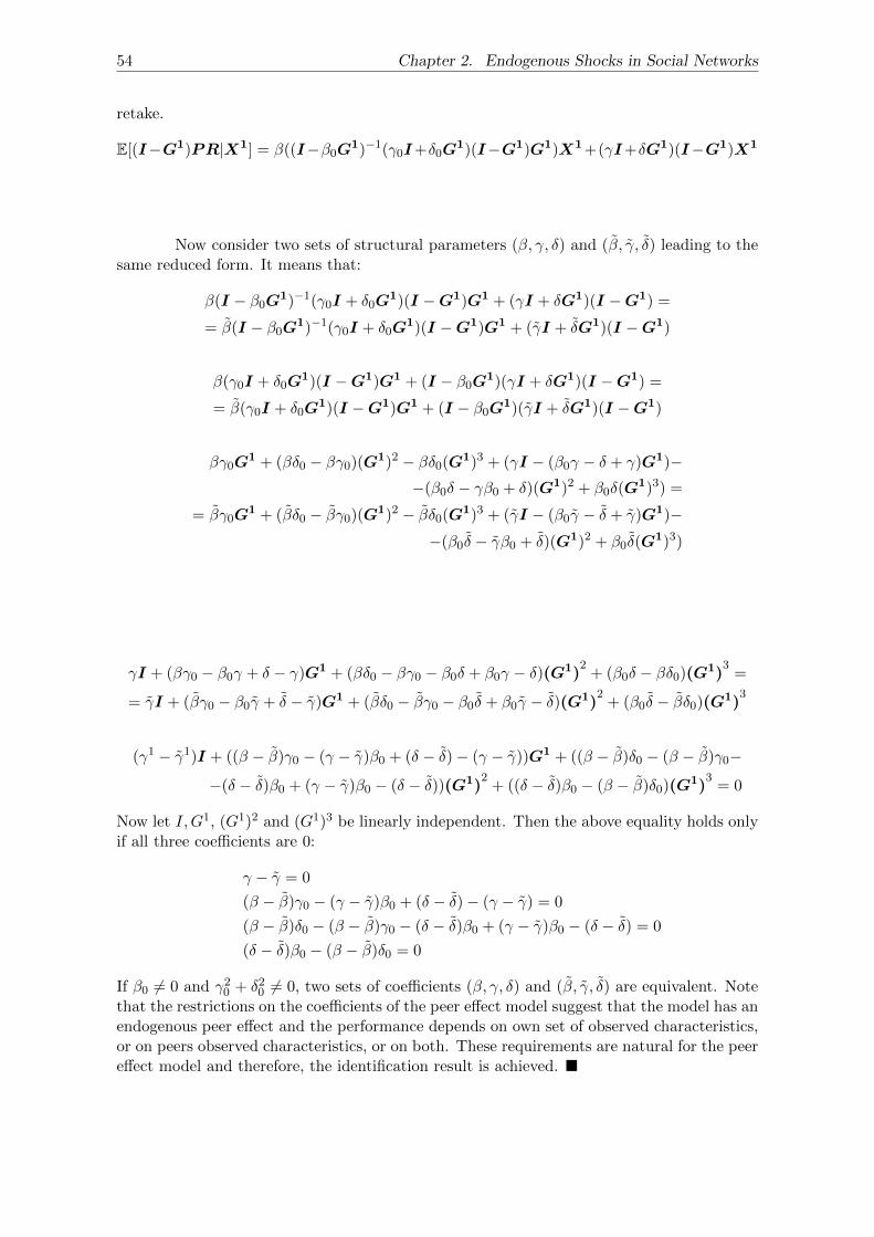
54 Chapter 2. Endogenous Shocks in Social Networks
retake.
E[(I−G1)PR|X1] = β((I−β0G1)−1(γ0I+δ0G1)(I−G1)G1)X1+(γI+δG1)(I−G1)X1
Now consider two sets of structural parameters (β, γ, δ) and (β, γ, δ) leading to thesame reduced form. It means that:
β(I − β0G1)−1(γ0I + δ0G1)(I −G1)G1 + (γI + δG1)(I −G1) =
= β(I − β0G1)−1(γ0I + δ0G1)(I −G1)G1 + (γI + δG1)(I −G1)
β(γ0I + δ0G1)(I −G1)G1 + (I − β0G1)(γI + δG1)(I −G1) =
= β(γ0I + δ0G1)(I −G1)G1 + (I − β0G1)(γI + δG1)(I −G1)
βγ0G1 + (βδ0 − βγ0)(G1)2 − βδ0(G1)3 + (γI − (β0γ − δ + γ)G1)−
−(β0δ − γβ0 + δ)(G1)2 + β0δ(G1)3) =
= βγ0G1 + (βδ0 − βγ0)(G1)2 − βδ0(G1)3 + (γI − (β0γ − δ + γ)G1)−
−(β0δ − γβ0 + δ)(G1)2 + β0δ(G1)3)
γI + (βγ0 − β0γ + δ − γ)G1 + (βδ0 − βγ0 − β0δ + β0γ − δ)(G1)2
+ (β0δ − βδ0)(G1)3
=
= γI + (βγ0 − β0γ + δ − γ)G1 + (βδ0 − βγ0 − β0δ + β0γ − δ)(G1)2
+ (β0δ − βδ0)(G1)3
(γ1 − γ1)I + ((β − β)γ0 − (γ − γ)β0 + (δ − δ)− (γ − γ))G1 + ((β − β)δ0 − (β − β)γ0−
−(δ − δ)β0 + (γ − γ)β0 − (δ − δ))(G1)2
+ ((δ − δ)β0 − (β − β)δ0)(G1)
3= 0
Now let I,G1, (G1)2 and (G1)3 be linearly independent. Then the above equality holds onlyif all three coefficients are 0:
γ − γ = 0
(β − β)γ0 − (γ − γ)β0 + (δ − δ)− (γ − γ) = 0
(β − β)δ0 − (β − β)γ0 − (δ − δ)β0 + (γ − γ)β0 − (δ − δ) = 0
(δ − δ)β0 − (β − β)δ0 = 0
If β0 6= 0 and γ20 + δ20 6= 0, two sets of coefficients (β, γ, δ) and (β, γ, δ) are equivalent. Notethat the restrictions on the coefficients of the peer effect model suggest that the model has anendogenous peer effect and the performance depends on own set of observed characteristics,or on peers observed characteristics, or on both. These requirements are natural for the peereffect model and therefore, the identification result is achieved. �

Appendix 55
Proof of Lemma 4. (Identification, Step 2, correlated effects)
The proof for Lemma 4 follows directly by applying similar arguments to the proofsof Lemma 2 and Lemma 3. Then, the identification is achieved under the conditions of linearindependence of I,G1, (G1)2, (G1)3 and I,G2, (G2)2, (G2)3 and G1 6= G2 and the follow-ing assumptions on the coefficients: β0,1 6= 0, γ20,1 + δ20,1 6= 0, β0,2 6= 0 and γ20,2 + δ20,2 6= 0. �
Proof of Lemma 5. Consistency of θLee of Step 1
√n(θLee − θ) = (
1
nZTX1)−1
1√nZTPR−
√nθ = (
1
nZTX1)−1(
1√nZTPR− 1√
nZTX1θ)
Then we can rewrite the last term:
1√nZTPR− 1√
nZTX1θ =
1√nZT
(PR−X1θ) =1√nZT
(αi+βG1y1+(γI+δG1)X1+ν−
−(αi+ (γI + δG1)X1 + βG1y1)) =1√nZTν
Hence,√n(θLee − θ) = (
1
nZTX1)−1
1√nZTν
Then the following two statements can be shown under the assumed regularity conditionsand by direct application of Lemmas A.7, A.8 and A.9 in L. Lee (2003):
plim1
nZTX1 = plim
1
nZTZ = J
1√nZTν
D−→ N (0, σ2νJ)
which will yield the desired result. �
Proof of Lemma 6. Consistency of φLee of Step 2
√n(φLee−φ) = (
1
nˆZTX)−1
1√n
ˆZT
(y2 − y1)−√nφ = (
1
nˆZTX)−1(
1√n
ˆZT
(y2 − y1)− 1√n
ˆZTXφ)
Then we can rewrite the last term:
1√n
ˆZT
(y2 − y1)− 1√n
ˆZTXφ =
1√n
ˆZT
(y2 − y1 − Xφ) =1√n
ˆZT
((α2 − α1)i+ β2G2y2−
−β1G1y1+δUR+γ2X2TV −γ1X
1TV +δ2G
2X2−δ1G1X1+∆ε−((α2−α1)i+β2G2y2−β1G1y1+
+δUR+ γ2X2TV − γ1X
1TV + δ2G
2X2 − δ1G1X1) =1√n
ˆZT
∆ε
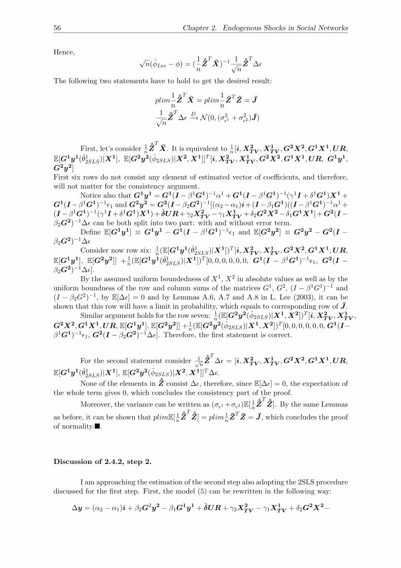
56 Chapter 2. Endogenous Shocks in Social Networks
Hence,√n(φLee − φ) = (
1
nˆZTX)−1
1√n
ˆZT
∆ε
The following two statements have to hold to get the desired result:
plim1
nˆZTX = plim
1
nZTZ = J
1√n
ˆZT
∆εD−→ N (0, (σ2ε1 + σ2ε2)J)
First, let’s consider 1n
ˆZTX. It is equivalent to 1
n [i,X2TV ,X
1TV ,G
2X2,G1X1,UR,
E[G1y1(θ12SLS)|X1], E[G2y2(φ2SLS)|X2,X1]]T [i,X2TV ,X
1TV ,G
2X2,G1X1,UR, G1y1,G2y2]First six rows do not consist any element of estimated vector of coefficients, and therefore,will not matter for the consistency argument.
Notice also that G1y1 = G1(I − β1G1)−1α1 +G1(I − β1G1)−1(γ1I + δ1G1)X1 +G1(I−β1G1)−1ε1 and G2y2 = G2(I−β2G2)−1[(α2−α1)i+(I−β1G1)((I−β1G1)−1α1 +(I−β1G1)−1(γ1I+ δ1G1)X1) + δUR+γ2X
2TV −γ1X1
TV + δ2G2X2− δ1G1X1] +G2(I−
β2G2)−1∆ε can be both split into two part: with and without error term.
Define E[G1y1] ≡ G1y1 − G1(I − β1G1)−1ε1 and E[G2y2] ≡ G2y2 − G2(I −β2G
2)−1∆εConsider now row six: 1
n(E[G1y1(θ12SLS)|X1])T [i,X2TV ,X
1TV ,G
2X2,G1X1,UR,
E[G1y1], E[G2y2]] + 1n(E[G1y1(θ12SLS)|X1])T [0, 0, 0, 0, 0, 0, G1(I − β1G1)−1ε1, G
2(I −β2G
2)−1∆ε].By the assumed uniform boundedness of X1, X2 in absolute values as well as by the
uniform boundness of the row and column sums of the matrices G1, G2, (I − β1G1)−1 and(I − β2G2)−1, by E[∆ε] = 0 and by Lemmas A.6, A.7 and A.8 in L. Lee (2003), it can beshown that this row will have a limit in probability, which equals to corresponding row of J .
Similar argument holds for the row seven: 1n(E[G2y2(φ2SLS)|X1,X2])T [i,X2
TV ,X1TV ,
G2X2,G1X1,UR, E[G1y1], E[G2y2]] + 1n(E[G2y2(φ2SLS)|X1,X2])T [0, 0, 0, 0, 0, 0,G1(I−
β1G1)−1ε1, G2(I − β2G2)−1∆ε]. Therefore, the first statement is correct.
For the second statement consider 1√n
ˆZT
∆ε = [i,X2TV ,X
1TV ,G
2X2,G1X1,UR,
E[G1y1(θ12SLS)|X1], E[G2y2(φ2SLS)|X2,X1]]T∆ε.
None of the elements in ˆZ consist ∆ε, therefore, since E[∆ε] = 0, the expectation ofthe whole term gives 0, which concludes the consistency part of the proof.
Moreover, the variance can be written as (σε1 +σε2)E[ 1nˆZT ˆZ]. By the same Lemmas
as before, it can be shown that plimE[ 1nˆZT ˆZ] = plim 1
nZTZ = J , which concludes the proof
of normality.�.
Discussion of 2.4.2, step 2.
I am approaching the estimation of the second step also adopting the 2SLS procedurediscussed for the first step. First, the model (5) can be rewritten in the following way:
∆y = (α2 − α1)i+ β2G2y2 − β1G1y1 + δUR+ γ2X
2TV − γ1X
1TV + δ2G
2X2−
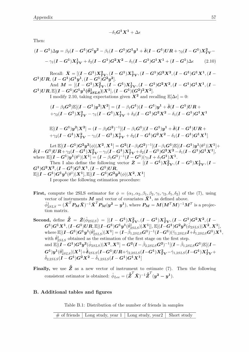
Appendix 57
−δ1G1X1 + ∆ε
Then:
(I −G1)∆y = β2(I −G1)G2y2 − β1(I −G1)G1y1 + δ(I −G1)UR+ γ2(I −G1)X2TV −
− γ1(I −G1)X1TV + δ2(I −G1)G2X2 − δ1(I −G1)G1X1 + (I −G1)∆ε (2.10)
Recall: X = [(I −G1)X2TV , (I −G1)X1
TV , (I −G1)G2X2, (I −G1)G1X1, (I −G1)UR, (I −G1)G1y1, (I −G1)G2y2].
And M = [(I − G1)X2TV , (I − G1)X1
TV , (I − G1)G2X2, (I − G1)G1X1, (I −G1)UR,E[(I −G1)G1y1(θ12SLS)|X1], (I −G1)(G2)2X2].
I modify 2.10, taking expectations given X2 and recalling E[∆ε] = 0:
(I − β2G2)E[(I −G1)y2|X2] = (I − β1G1)(I −G1)y1 + δ(I −G1)UR+
+γ2(I −G1)X2TV − γ1(I −G
1)X1TV + δ2(I −G1)G2X2 − δ1(I −G1)G1X1
E[(I −G1)y2|X2] = (I − β2G2)−1[(I − β1G1)(I −G1)y1 + δ(I −G1)UR+
+γ2(I −G1)X2TV − γ1(I −G
1)X1TV + δ2(I −G1)G2X2 − δ1(I −G1)G1X1]
Let E[(I−G1)G2y2(φ)|X2,X1] = G2(I−β2G2)−1[(I−β1G1)E[(I−G1)y1(θ1)|X1]+δ(I−G1)UR+γ2(I−G1)X2
TV −γ1(I−G1)X1TV +δ2(I−G1)G2X2−δ1(I−G1)G1X1],
where E[(I −G1)y1(θ1)|X1] = (I − β1G1)−1(I −G1)(γ1I + δ1G1)X1.
Then I also define the following vector Z = [(I − G1)X2TV , (I − G1)X1
TV , (I −G1)G2X2, (I −G1)G1X1, (I −G1)UR,E[(I −G1)G1y1(θ1)|X1],E[(I −G1)G2y2(φ)|X2,X1]
I propose the following estimation procedure:
First, compute the 2SLS estimator for φ = (α1, α2, β1, β2, γ1, γ2, δ1, δ2) of the (7), usingvector of instruments M and vector of covariates X1, as defined above.
φ12SLS = (XTPMX)−1X
TPM (y2 − y1), where PM = M(MTM)−1MT is a projec-
tion matrix.
Second, define ˆZ = Z(φ2SLS) = [(I − G1)X2TV , (I − G1)X1
TV , (I − G1)G2X2, (I −G1)G1X1, (I−G1)UR,E[(I−G1)G1y1(θ12SLS)|X1]], E[(I−G1)G2y2(φ2SLS)|X2,X1],
where E[(I−G1)G1y1(θ12SLS)|X1] = (I−β1,2SLSG1)−1(I−G1)(γ1,2SLSI+δ1,2SLSG1)X1,
with θ12SLS obtained as the estimation of the first stage on the first step.
and E[(I −G1)G2y2(φ2SLS)|X2,X1] = G2(I − β2,2SLSG2)−1[(I − β1,2SLSG1)E[(I −G1)y1(θ12SLS)|X1]+
ˆδ2SLS(I−G1)UR+γ2,2SLS(I−G1)X2
TV −γ1,2SLS(I−G1)X1TV +
δ2,2SLS(I −G1)G2X2 − δ1,2SLS(I −G1)G1X1]
Finally, we use ˆZ as a new vector of instrument to estimate (7). Then the following
consistent estimator is obtained: φLee = ( ˆZTX)−1 ˆZ
T(y2 − y1).
B. Additional tables and figures
Table B.1: Distribution of the number of friends in samples
# of friends Long study, year 1 Long study, year2 Short study
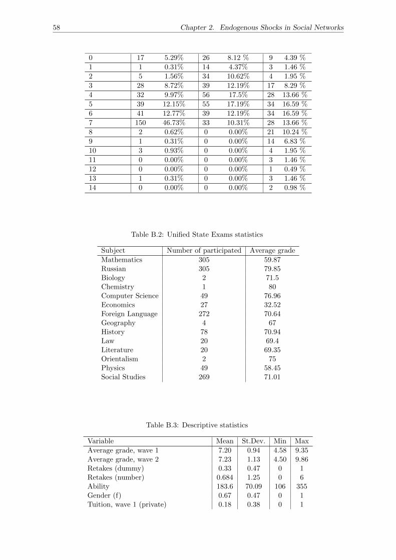
58 Chapter 2. Endogenous Shocks in Social Networks
0 17 5.29% 26 8.12 % 9 4.39 %
1 1 0.31% 14 4.37% 3 1.46 %
2 5 1.56% 34 10.62% 4 1.95 %
3 28 8.72% 39 12.19% 17 8.29 %
4 32 9.97% 56 17.5% 28 13.66 %
5 39 12.15% 55 17.19% 34 16.59 %
6 41 12.77% 39 12.19% 34 16.59 %
7 150 46.73% 33 10.31% 28 13.66 %
8 2 0.62% 0 0.00% 21 10.24 %
9 1 0.31% 0 0.00% 14 6.83 %
10 3 0.93% 0 0.00% 4 1.95 %
11 0 0.00% 0 0.00% 3 1.46 %
12 0 0.00% 0 0.00% 1 0.49 %
13 1 0.31% 0 0.00% 3 1.46 %
14 0 0.00% 0 0.00% 2 0.98 %
Table B.2: Unified State Exams statistics
Subject Number of participated Average grade
Mathematics 305 59.87Russian 305 79.85Biology 2 71.5Chemistry 1 80Computer Science 49 76.96Economics 27 32.52Foreign Language 272 70.64Geography 4 67History 78 70.94Law 20 69.4Literature 20 69.35Orientalism 2 75Physics 49 58.45Social Studies 269 71.01
Table B.3: Descriptive statistics
Variable Mean St.Dev. Min Max
Average grade, wave 1 7.20 0.94 4.58 9.35Average grade, wave 2 7.23 1.13 4.50 9.86Retakes (dummy) 0.33 0.47 0 1Retakes (number) 0.684 1.25 0 6Ability 183.6 70.09 106 355Gender (f) 0.67 0.47 0 1Tuition, wave 1 (private) 0.18 0.38 0 1
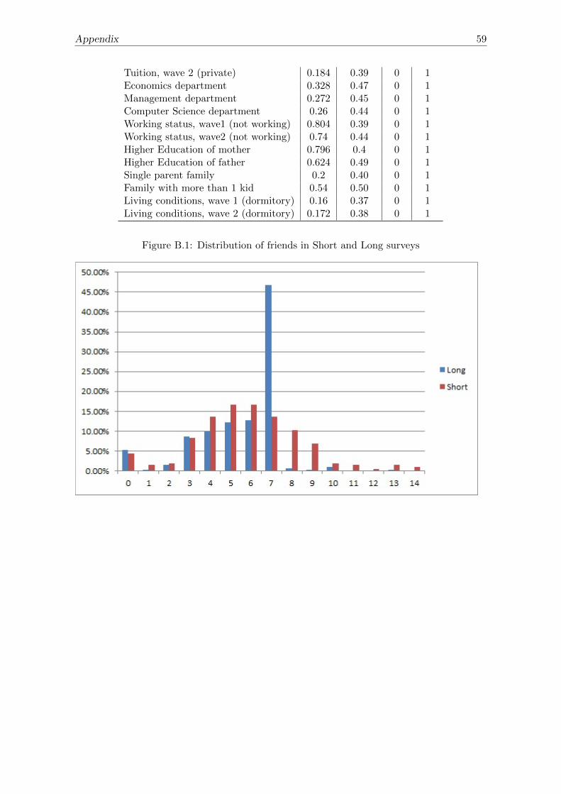
Appendix 59
Tuition, wave 2 (private) 0.184 0.39 0 1Economics department 0.328 0.47 0 1Management department 0.272 0.45 0 1Computer Science department 0.26 0.44 0 1Working status, wave1 (not working) 0.804 0.39 0 1Working status, wave2 (not working) 0.74 0.44 0 1Higher Education of mother 0.796 0.4 0 1Higher Education of father 0.624 0.49 0 1Single parent family 0.2 0.40 0 1Family with more than 1 kid 0.54 0.50 0 1Living conditions, wave 1 (dormitory) 0.16 0.37 0 1Living conditions, wave 2 (dormitory) 0.172 0.38 0 1
Figure B.1: Distribution of friends in Short and Long surveys
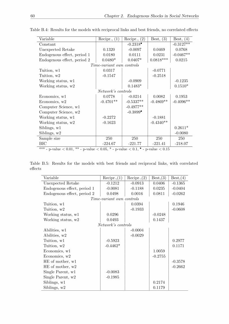
60 Chapter 2. Endogenous Shocks in Social Networks
Table B.4: Results for the models with reciprocal links and best friends, no correlated effects
Variable Recipr., (1) Recipr., (2) Best, (3) Best, (4)
Constant -0.2318• -0.3127**Unexpected Retake 0.1320 -0.0097 0.0469 0.0768Endogenous effect, period 1 0.0180 0.0111 0.0231 -0.0467**Endogenous effect, period 2 0.0480* 0.0407* 0.0818*** 0.0215
Time-variant own controlsTuition, w1 0.0317 -0.0771Tuition, w2 -0.1547 -0.2518Working status, w1 -0.0909 -0.1235Working status, w2 0.1483* 0.1510*
Network’s controlsEconomics, w1 0.0778 -0.0214 0.0082 0.1953Economics, w2 -0.4701** -0.5337** -0.4869** -0.4096**Computer Science, w1 -0.4977**Computer Science, w2 -0.3899•
Working status, w1 -0.2272 -0.1881Working status, w2 -0.1623 -0.4340**Siblings, w1 0.2611*Siblings, w2 -0.0080
Sample size 250 250 250 250BIC -224.67 -221.77 -221.41 -218.07
*** - p-value < 0.01, ** - p-value < 0.05, * - p-value < 0.1, • - p-value < 0.15
Table B.5: Results for the models with best friends and reciprocal links, with correlatedeffects
Variable Recipr.,(1) Recipr.,(2) Best,(3) Best,(4)
Unexpected Retake -0.1212 -0.0913 0.0406 -0.1365Endogenous effect, period 1 -0.0081 -0.1188 0.0235 -0.0404Endogenous effect, period 2 0.0498 0.0016 0.0811 -0.0262
Time-variant own controlsTuition, w1 0.0394 0.1946Tuition, w2 -0.1933 -0.0608Working status, w1 0.0296 -0.0248Working status, w2 0.0493 0.1437
Network’s controlsAbilities, w1 -0.0004Abilities, w2 -0.0029Tuition, w1 -0.5923 0.2977Tuition, w2 -0.4462* 0.1171Economics, w1 1.0059Economics, w2 -0.2755HE of mother, w1 -0.3578HE of mother, w2 -0.2662Single Parent, w1 -0.0083Single Parent, w2 -0.1985Siblings, w1 0.2174Siblings, w2 0.1179

Appendix 61
Sample size 250 250 250 250BIC -191.02 -192.71 -189.98 -183.06
*** - p-value < 0.01, ** - p-value < 0.05, * - p-value < 0.1, • - p-value < 0.15
Table B.6: List of classes with retakes in the sample
Class Department Total No. of retakes Important classes
Algebra Computer Science 21 NoArchitecture of ComputerSystems
Computer Science 2 No
Architecture of ECM Computer Science 1 NoBasics of computer technologyand programming
Computer Science 3 Yes
Discrete Mathematic Computer Science 8 NoDiscrete Mathematic Economics 2 NoEconomic Theory and Institu-tional Analysis
Management 28 (in 2 terms) Yes
Economic Theory and Institu-tional Analysis
Computer Science 12 No
Economic Theory Basics Economics 27 (in 3 terms) YesEconomics Computer Science 3 NoEnglish and other languages All departments 9 NoGeometry and Algebra Computer Science 8 YesHistory of economic thoughts Economics 1 YesHistory of foreign state andlaw
Law 2 Yes
Introduction to software engi-neering
Computer Science 3 Yes
Judicial power and law en-forcement
Law 1 No
Life safety All departments 3 NoLinear Algebra Economics 28 NoMathematical Analysis Computer Science 68 (in 2 terms) YesMathematical Analysis Economics 12 YesMathematics Management 31 (in 2 terms) YesMethods of financial and eco-nomic computations
Economics 1 No
Microeconomics Computer Science 18 (in 2 terms) YesPhilosophy Management 6 YesRoman Law Law 1 NoSocio-Economic Statistics Economics 2 NoSociology Management 1 YesTheoretical basics of com-puter technology
Computer Science 9 (in 2 terms) No
Theory of state and law Law 4 Yes
References, chapter 2
Ammermueller, A. and J.-S. Pischke (2009). “Peer effects in European primary schools:Evidence from the progress in international reading literacy study”. In: Journal of LaborEconomics 27.3, pp. 315–348.
Androushchak, Gregory, Oleg Poldin, and Maria Yudkevich (2013). “Role of peers in studentacademic achievement in exogenously formed university groups”. In: Educational Studies39.5, pp. 568–581.
Angrist, J.D. and K. Lang (2004). “Does school integration generate peer effects? Evidencefrom Boston’s Metco Program”. In: American Economic Review, pp. 1613–1634.
Aral, S., L. Muchnik, and A. Sundararajan (2009). “Distinguishing influence-based contagionfrom homophily-driven diffusion in dynamic networks”. In: Proceedings of the NationalAcademy of Sciences 106.51, pp. 21544–21549.
AUSTRALIA: High drop-out rates cost $1.4 billion (2010). url: http://www.universityworldnews.com/article.php?story=20101022203542738.
Battin-Pearson, S. et al. (2000). “Predictors of early high school dropout: A test of fivetheories.” In: Journal of educational psychology 92.3, pp. 568–582.
Bramoulle, Y., H. Djebbari, and B. Fortin (2009). “Identification of peer effects throughsocial networks”. In: Journal of econometrics 150.1, pp. 41–55.
Buchmann, Claudia and Ben Dalton (2002). “Interpersonal influences and educational aspira-tions in 12 countries: The importance of institutional context”. In: Sociology of education75, pp. 99–122.
Calvo-Armengol, A., E. Patacchini, and Y. Zenou (2009). “Peer effects and social networksin education”. In: The Review of Economic Studies 76.4, pp. 1239–1267.
Carrell, S.E., R.L. Fullerton, and J.E. West (2009). “Does your cohort matter? Measuringpeer effects in college achievement”. In: Journal of Labor Economics 27.3, pp. 439–464.
Chandrasekhar, A. and R. Lewis (2011). “Econometrics of sampled networks”. In: Unpub-lished manuscript, MIT.[422].
Coleman, J.S. (1990). Foundations of social theory. Harvard university press.Comola, M. and S. Prina (2014). “Do interventions change the network? A dynamic peer
effect model accounting for network changes”. In: Working paper.De Giorgi, Giacomo, Michele Pellizzari, and Silvia Redaelli (2010). “Identification of social
interactions through partially overlapping peer groups”. In: American Economic Journal:Applied Economics, pp. 241–275.
Elhorst, J. Paul (2010). “Dynamic panels with endogenous interaction effects when T issmall”. In: Regional Science and Urban Economics 40.5, pp. 272–282.
French, D.C. and J. Conrad (2001). “School dropout as predicted by peer rejection andantisocial behavior”. In: Journal of Research on adolescence 11.3, pp. 225–244.
Gardner, Michael (2007). GERMANY: Heavy cost of student drop-outs. url: http://www.universityworldnews.com/article.php?story=20071025102357719.
62

REFERENCES, CHAPTER 2 63
Garnier, H.E., J.A. Stein, and J.K. Jacobs (1997). “The process of dropping out of highschool: A 19-year perspective”. In: American Educational Research Journal 34.2, pp. 395–419.
Gaviria, A. and S. Raphael (2001). “School-based peer effects and juvenile behavior”. In:Review of Economics and Statistics 83.2, pp. 257–268.
Goldsmith-Pinkham, P. and Guido W Imbens (2013). “Social networks and the identificationof peer effects”. In: Journal of Business & Economic Statistics 31.3, pp. 253–264.
Hanushek, E.A. et al. (2003). “Does peer ability affect student achievement?” In: Journal ofapplied econometrics 18.5, pp. 527–544.
Hoxby, C. (2000). Peer effects in the classroom: Learning from gender and race variation.Tech. rep. National Bureau of Economic Research.
Indicators of economics of education, url: https://memo.hse.ru/ind.Jackson, Matthew O. (2010). “An overview of social networks and economic applications”.
In: The handbook of social economics 1, pp. 511–585.Kelejian, Harry H and Ingmar R Prucha (1998). “A generalized spatial two-stage least
squares procedure for estimating a spatial autoregressive model with autoregressive dis-turbances”. In: The Journal of Real Estate Finance and Economics 17.1, pp. 99–121.
Lee, Lungfei (2003). “Best Spatial Two-Stage Least Squares Estimators for a Spatial Au-toregressive Model with Autoregressive Disturbances”. In: Econometric Reviews 22.4,pp. 307–335.
Lomi, A. et al. (2011). “Why are some more peer than others? Evidence from a longitudi-nal study of social networks and individual academic performance”. In: Social ScienceResearch 40.6, pp. 1506–1520.
Manski, C.F. (1993). “Identification of endogenous social effects: The reflection problem”.In: The review of economic studies 60.3, pp. 531–542.
McPherson, M., L. Smith-Lovin, and J. M. Cook (2001). “Birds of a feather: Homophily insocial networks”. In: Annual review of sociology, pp. 415–444.
Metco program official webpage. url: http://www.doe.mass.edu/metco/.Newcomb, M.D. (1996a). “Adolescence: Pathologizing a normal process.” In: The counseling
Psychologist 24, pp. 482–490.— (1996b). “Pseudomaturity among adolescents: Construct validation, sex differences, and
associations in adulthood.” In: Journal of Drug Issues 26, pp. 477–504.Paula, Aureo de (2015). “Econometrics of Network Models”. In: cemmap Working paper
CWP52/15.Poldin, Oleg, Diliara Valeeva, and Maria Yudkevich (2015). “Which Peers Matter: How Social
Ties Affect Peer-group Effects”. In: Research in Higher Education, pp. 1–21.Rumberger, R.W. (1983). “Dropping out of high school: The influence of race, sex, and family
background”. In: American Educational Research Journal.Sacerdote, B. (2011). “Peer effects in education: How might they work, how big are they
and how much do we know thus far?” In: Handbook of the Economics of Education 3,pp. 249–277.
Sacerdote, Bruce (2001). “Peer Effects with Random Assignment: Results for DartmouthRoommates”. In: Quartetly Journal of Economics 116.2, pp. 681–704.
Shugal, N. (2010). “Potoki obuchayushchikhsya v rossiyskoy sisteme obrazovaniya [Studentflows in Russian education system]”. In: Voprosy obrazovaniya / Educational Studies 4,pp. 122–148.
Smith, J.P. and R.A. Naylor (2001). “Dropping Out of University: A Statistical Analysisof the Probability of Withdrawal for UK University Students”. In: Journal of the RoyalStatistical Society. Series A (Statistics in Society) 164.2, pp. 389–405.

64 REFERENCES, CHAPTER 2
Socio-Economic situation in Russia (2014). url: http://www.gks.ru/bgd/regl/b14_01/Main.htm.
Stinebrickner, T. and R. Stinebrickner (2013). Academic performance and college dropout:Using longitudinal expectations data to estimate a learning model. Tech. rep. NationalBureau of Economic Research.
Tinto, V. (1975). “Dropout from higher education: A theoretical synthesis of recent research”.In: Review of educational research, pp. 89–125.
Triandis, Harry C (1989). “The self and social behavior in differing cultural contexts.” In:Psychological review 96.3, pp. 506–520.
Chapter 3
Peer effects in art prices
3.1 Introduction
Art is receiving an increased attention in recent years as a possible investment. Art is
often attributed to the category of so-called passion investment, which also includes jewelry,
antiques, classic car, wine, etc. Passion investments are assessed to amount to 6% of total
wealth (The Wall Street Journal, 2010), and the high-net-worth investors allocate globally
around 17% of their cash to art (World Wealth Report 2013). According to Knight Frank
Luxury Investment Index 2014, the 10-year capital appreciation of art is among highest and
equal to 226%1. The estimation of the real returns in existing literature varies, depending
on the methodology, time period and data used. For example, Goetzmann (1993) reports an
average annual real return on oil paintings of 3.8% for the period between 1850 and 1986,
with returns around 15% after 1940. Mei and Moses (2002) calculate the return of 4.9% for
1875-1999, with 8.2% after 1950. Renneboog and Spaenjers (2013) are more careful in their
estimation with 3.97% over the period 1957-2007.
However, some of these results show the underperformance of art in comparison to
the other types of investments. Moreover, the volatility of the prices on the art market is
rather high. The attractiveness of the art market is, therefore, cannot be explained by the
investment purposes. Global art and antique sales are steadily high in the last several years
and are close to 50 billion Euro (with the exception of 2009 crisis)2. Buying pieces of art
is also a popular tendency among high earners. Owning the work by a famous artist may
help to strengthen a status in the society. Creating one’s own collection can yield additional
respect for their owner. The attractiveness of the art market in comparison to the other
luxury items, as stated in the World Wealth Report 2013, is likely ”driven by auction house
sales, the art market is lively compared to other categories that are characterized more by
inheritance and private sales”. Approximately half of the art sales are made via auctions
(McAndrew 2010), the rest are privately traded, mostly via art dealers. The auction prices
1Consult here for more details.2European Fine Art Foundation report
65

66 Chapter 3. Peer effects in art prices
are the ones who set the benchmark for the art prices in general.
In the literature, discussing art pricing, the following standard set of variables is
usually used as determinants of the price: artists’ characteristics, works’ characteristics, such
as medium, authenticity, attribution, size, and topic, as well as the sales characteristics, such
as a date and a place. Artists’ reputation is usually included, however, it is not always clear,
how to account for it. Renneboog and Spanjers (2012) include a dummy for mentioning of
the artist in the classic art history textbook ”Gardner’s Art Through Ages” and a dummy
of exhibiting at Dokumenta in Kassel.
This paper explores one important determinant of the art price formation that is
potentially missing in the existing analysis, namely the artists’ connections. I believe that
connections can influence in two ways. First of all, following the classical peer effect logic,
artists’ links are influencing the development of artists’ style and quality of the works. But
also the prices of the work of one artist may be driven by the prices of the connected
artists. If the artists worked together or were connected by the same movement, it is likely
that their works will resemble some similarities and may get similar prices on the market.
Alternatively, the demand for some artist’s works may increase, increasing the price, if the
works of connected to them artist are not available or too expensive. The famous film about
street artist Banksy, ”Exit through the Gift Shop”, also depicts, how connections can attract
high demand and big money to quite mediocre pieces of art. The paper uses the data on
abstract movement artists and their works, collected especially for this project from the open
resources. Abstract art is, along with contemporary art, among the movements, for which
the price is especially difficult to determine, and hence, exploring the new channels of price
formation may help to understand it better.
I apply the peer effect model introduced by Manski (1993) to the panel data on the
prices of abstract artists’ work sold at Sotheby’s in 2000-first half of 2015. Although the
model is modified to be applied to the panel data, and to use price as an individual outcome
variable and average price as an endogenous variable of the connections, the identifying
assumptions of Bramoulle, Djebbari, and Fortin (2009) are still valid. The network is required
to have intransitive triads for the model without the correlated effect and the connections
of length 3 for the model with correlated effects. This means that there should exist two
artists that are not connected directly, but via one more artist (or two). These assumptions
are plausible for most of the networks, and for the network of abstract artists in particular.
The paper is organized as follows. Section 2 discusses the proposed peer effect model
and suggested estimation method. Section 3 introduces the data and provides some of the
descriptive analysis. Section 4 provides the empirical results. Section 5 concludes.
3.2 Model
I have the sample of all works sold at Sotheby’s for all of the artists in the sample,
for i ∈ [1, I] being an artwork from the whole set, j ∈ [1, J ] being an artist, created the work.
In order to estimate the effect of being connected to other artists on prices of own work, I

3.2. Model 67
am proposing the model of peer effect, similar to Manski (1993) and Bramoulle, Djebbari,
and Fortin (2009), with the slight appropriate modification:
P ji = α0 + α1ti + β0Zi + β1Xj + β2∑l 6=j
GjlXl + γ∑l 6=j
GjlPl + νj + εji (3.1)
Some comments on the model ingredients are necessary.
P ji - price of the piece i by artist j. The prices are normalized as will be discussed in the
next section.
Zi - are the characteristics of the painting, that may include type of the work, size, possibly
attribution to an artists’ important period, provenance or exhibition history3.
Xj , Xl - are the characteristics of the artists, such as particular style, major work type (paint-
ings, sculpture etc.), country of birth and living, years active, possibly the total amount of
works produced.
Gjl - is adjacency matrix with 1/nj in the jl cell, if an artist j is connected with an artist
l, with nj being the total number of connections of an artist j. Note that, although all the
links are reciprocal in this particular setting, the matrix is not symmetrical, since
nu.j - are the unobserved effects of the artists.
Here β2 represents exogenous effect, how the similar characteristics of the connec-
tions influence the outcomes, γ is endogenous effect, showing how the outcomes of the con-
nections may influence the outcome of the individual, νj are the unobserved characteristics
of particular painter in the panel.
The presence of individual unobservable effect creates additional issue for the iden-
tification of the endogenous effects.
Potentially, the correlated effects can be also present in the model, making the
smaller group within the network to behave similarly due to the unobserved similarities of
the group. However, the network used in this paper is rather small, and the potential simi-
larities of the subgroup can be captured by observed characteristics, such as the country of
origin or/and work, the group affiliation etc. In more general setting the correlated effects
problem can be dealt with by applying the local differences, averaging over the first level
connections’ outcome variables. The identification of endogenous effect is then achieved by
the presence of links of the length 3 or more, and so G3jlXl can be used as identifying instru-
ments for the endogenous covariates.
Since the network is held constant in the panel, the fixed effects model, that is more
suitable from the empirical point of view, is not applicable, as then the endogenous effect
cannot be identified. So either the unobserved individual effects should be treated by random
effects analysis or Hausman and Taylor type models should be used.
Both possibilities are plausible, depending on the explanation of assumptions one
believes in. The unobserved individual effects in our empirical could represent the level of
talent of the particular artist, his/her popularity, as well as characteristics not included or
3The variables will be discussed in details in later sections
68 Chapter 3. Peer effects in art prices
missing in the vector of covariates attributed to the artist that could influence the outcome
variable. The level of talent and some potential covariates are more likely to be uncorrelated
with explanatory variables. The popularity is, however, possibly correlated with one of the
explanatory variables, in particular, with the characteristics and outcomes of the connec-
tions. In this case, the random effects will produce inconsistent estimators of all parameters,
and the Hausman and Taylor type models are more suitable for this particular setting. It is,
however, more computationally demanding, and once the correlation is absent, the random
effects are preferable.
3.2.1 Hausman and Taylor type models
If it is suspected that individual unobservables are correlated with the explanatory
variables and time-constant4 variables are of interest, as was already mentioned, neither fixed
effects nor random effects are suitable for the analysis.
For now, I will ignore the correlated effects for simplicity of explaining the estimation
approach. I will give a note on adding the correlated effects in the model later in the paper.
First, I divide all explanatory variables into two vectors: time-variant Zji = {ti, Zji } and
time-constant Xj = {1, Xj ,∑
l 6=j GjlXl,∑
l 6=j GjlPl}. I follow Hausman and Taylor (1981)
approach and partition both vectors as follows: Zji = (Zj
i1,Zji2) andXj = (Xj1,Xj2) where
Zji1 is 1×K1, Z
ji2 is 1×K2, Xj1 is 1× J1, Xj2 is 1× J2 and the following assumptions are
fulfilled:
E(Xj1νj) = 0 and E(Zji1νj) = 0
Additionally, the following assumption is necessary:
E(εji |Xj ,Zj1, . . . ,Z
jwj, νj) = 0, i = 1, . . . , wj
with wj being the number of works of artist j in the sample.
We can then rewrite the original model in a simpler way:
P ji = βZji + αXj + νj + εji (3.2)
where β = (α1, β0) and α = (α0, β1, β2, γ).
Note that under assumptions in this subsections the time-constant variables are
likely to include the outcome variable of friends, which are endogenous in the model. There-
fore, the vector of instruments necessary to apply HT approach should additionally include
an identifying instrument for the endogenous peer effect, which is the exogenous character-
istics of friends of friends, following Bramoulle, Djebbari, and Fortin (2009). The estimation
procedure is as follows:
• First, the fixed effects approach is applied, which gives consistent estimation of the
4Note, that notion of time is used here not in the direct sense, but rather follows the conventional termi-nology of panel data analysis. Time here denotes each time one of the works was auctioned.
3.2. Model 69
coefficients of the time-varying variables βFE .
• Using the estimator of the first step, calculate the residuals as follows:
dj = P j − βFEZj = αXj + νj + εj (3.3)
• Now, estimate 3.3 with a 2SLS approach. The standard vector of instruments in
Hausman and Taylor approach is [Zji1,Xj1]. To be able to identify the endogenous
peer effect, I suggest adding∑
l 6=j Gjl∑
k 6=lGlkXk to vector of instruments.
• Using the residual variance σ∗2 from the previous step and estimator of σ2ε from the
first step, calculate σ2ν = σ∗2−σ2ε /T , where T is a harmonic mean of Tj ’s. And compute
the weighting coefficients for GLS as:
θj = 1− (σ2ε
σ2ε + Tjσ2ν)0.5
• Finally, the following transformations are made: P j∗i = P ji − θjP j , Zj∗i = Zji − θjZj ,
Xj∗ = Xj − θjX. IV regression of P j∗i on Zj∗i , Xj∗ are performed, using the vector of
instruments [Zji − Zj , Zji1, Xj1,
∑l 6=j Gjl
∑k 6=lGlkXk]
3.2.2 Alternative approach
The Hausman and Taylor approach is computationally challenging, and the number
of artists in the sample is not very high with the number of observations for each of them
varies a lot, therefore, the alternative approach, avoiding usage of panel data structure is
also proposed. The artists dummies are used in this case, combined with the standard 2SLS
proposed by Bramoulle, Djebbari, and Fortin (2009) following L. Lee (2003) approach. The
model is then as follows:
P ji = α0 + α1ti + α2ADi + β0Zi + β1Xj + β2∑l 6=j
GjlXl + γ∑l 6=j
GjlPl + εji (3.4)
with ADi - set of artists’ dummies.
The 2SLS is then conducted with∑
l 6=j Gjl∑
k 6=lGlkXk as an instrument for an
endogenous variable∑
l 6=j GjlPl.
The two proposed approaches should yield comparable results since both of them
provide consistent estimators. I do not prove the consistency of the resulting estimators in
this paper, but it logically follows from the proofs in Hausman and Taylor (1981) and L. Lee
(2003).
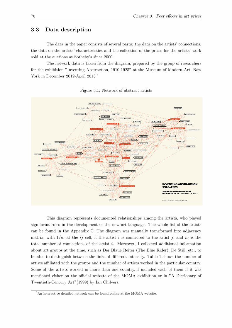
70 Chapter 3. Peer effects in art prices
3.3 Data description
The data in the paper consists of several parts: the data on the artists’ connections,
the data on the artists’ characteristics and the collection of the prices for the artists’ work
sold at the auctions at Sotheby’s since 2000.
The network data is taken from the diagram, prepared by the group of researchers
for the exhibition ”Inventing Abstraction, 1910-1925” at the Museum of Modern Art, New
York in December 2012-April 2013.5
Figure 3.1: Network of abstract artists
This diagram represents documented relationships among the artists, who played
significant roles in the development of the new art language. The whole list of the artists
can be found in the Appendix C. The diagram was manually transformed into adjacency
matrix, with 1/ni at the ij cell, if the artist i is connected to the artist j, and ni is the
total number of connections of the artist i. Moreover, I collected additional information
about art groups at the time, such as Der Blaue Reiter (The Blue Rider), De Stijl, etc., to
be able to distinguish between the links of different intensity. Table 1 shows the number of
artists affiliated with the groups and the number of artists worked in the particular country.
Some of the artists worked in more than one country, I included each of them if it was
mentioned either on the official website of the MOMA exhibition or in ”A Dictionary of
Twentieth-Century Art”(1999) by Ian Chilvers.
5An interactive detailed network can be found online at the MOMA website.

3.3. Data description 71
Table 3.1: Countries and groups allocation
Countries Groups
France (30), USA (20), Germany (18),
Russia (18), Italy (15), Switzerland (9),
England (8), Poland (5), Spain (4), The
Netherlands (4), Hungary (3), Romania
(2)
Der Blaue Reiter (7), Puteaux Group (6),
De Stijl (4), Union of Youth (4), Donkey’s
Tail (3), Supremus (3), 291 Gallery (3),
Jack of Diamonds (2), Societe Anonyme
(2), Bloomsbury group (2)
The existing network determined the sample of the artists used for the analysis.
However, several of the names from the list were not included in the analysis. Those are
people important for the abstraction movement, but they were not creative artists, such as,
for example, Guillaume Apollinaire, who was a writer and an art critic, or Claude Debussy,
who was a composer. Therefore, the auctioned items related to these people are more likely
to be personal items or similar. There are 83 artists in the initial list, 11 of which were
eliminated.
The set of artists’ characteristics were collected from different biographical sources.
Among those characteristics are the following: years of life and years active, the country
of birth and the country, where the artist was more active, main artistic mode (paintings,
sculpture, photographs etc.), particular major style inside of abstractionism; if available,
approximate amount of known works and most valuable periods to be able to determine the
rarity of the works.
The price dataset was collected specially for this paper from the Sotheby’s auction
house website. The special program was written to obtain all the lots for each of the artists,
auctioned at Sotheby’s and both sold and not. The data were available for the auctions that
took place from the year 2000, earlier lots are not available online. For each lot the following
information is usually available: an estimated price of the work, whether it was sold and the
price, which lot was sold, date of creation, type of work, size, provenance, history of exhi-
bitions, although the descriptive information is missing in quite a lot of cases. There might
also be some additional catalogue notes, including conditions, authenticity information, etc.
However, not all of this information can be included in the model. Part of the description is
very difficult to re-translate into quantitative variables.
There are several data issues that should be pointed out. First of all, for now only
the data from one auction house is used. This may cause some distortion of the results since
I am not looking at the whole market situation, i.e. I am not controlling for the availability
of the works of a particular artist in the other auction house at the same time. The full
dataset will be collected in the future research, however, new programs should be written for
each of the auction houses to scrap the data from their websites due to the different layouts.
Secondly, the types of works included in the sample are rather different, such as oil
paintings, watercolours, lithographs, different types of sculptures, photographs etc. Includ-
ing dummies for each of the type of the work is possible. However, the description is missing
for almost 30% of the cases, hence, not all of the works can be attributed to a particular
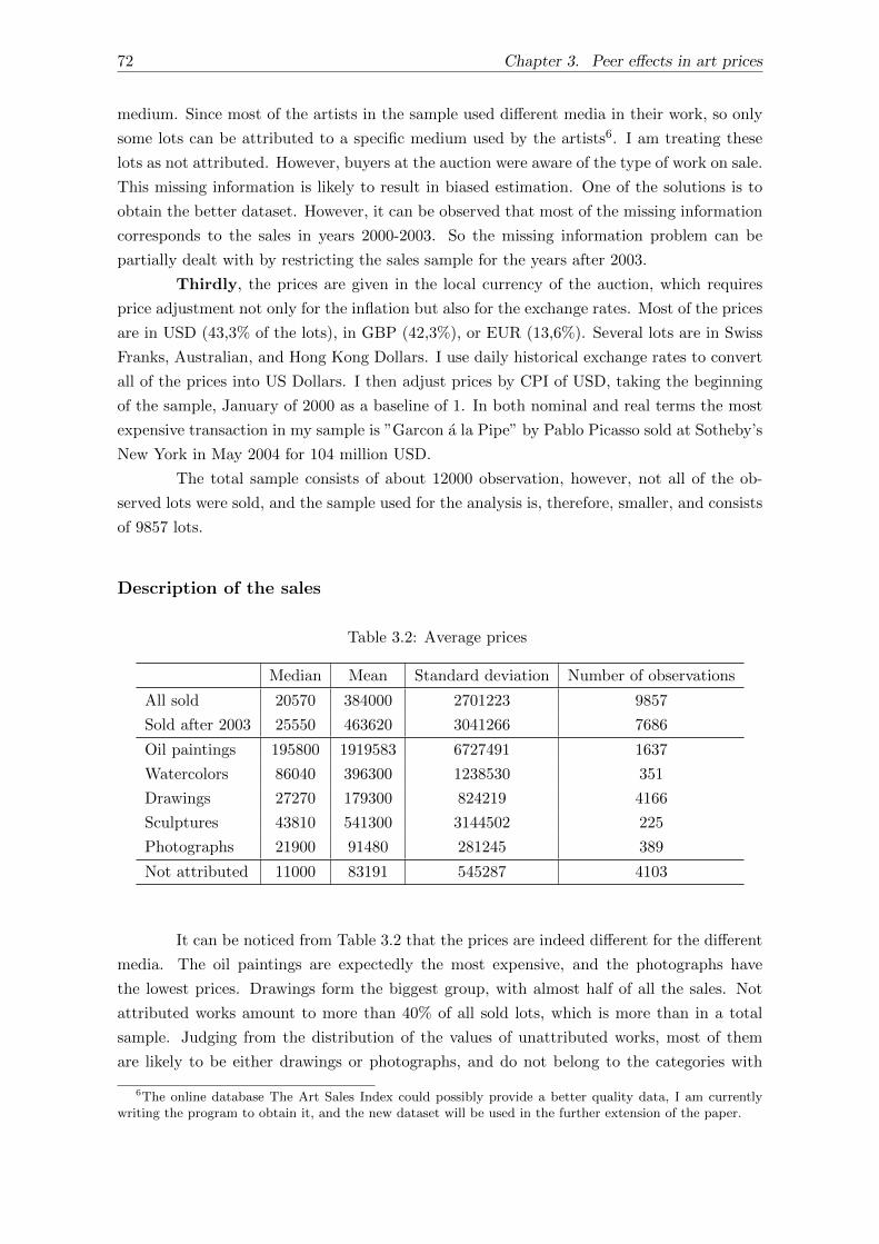
72 Chapter 3. Peer effects in art prices
medium. Since most of the artists in the sample used different media in their work, so only
some lots can be attributed to a specific medium used by the artists6. I am treating these
lots as not attributed. However, buyers at the auction were aware of the type of work on sale.
This missing information is likely to result in biased estimation. One of the solutions is to
obtain the better dataset. However, it can be observed that most of the missing information
corresponds to the sales in years 2000-2003. So the missing information problem can be
partially dealt with by restricting the sales sample for the years after 2003.
Thirdly, the prices are given in the local currency of the auction, which requires
price adjustment not only for the inflation but also for the exchange rates. Most of the prices
are in USD (43,3% of the lots), in GBP (42,3%), or EUR (13,6%). Several lots are in Swiss
Franks, Australian, and Hong Kong Dollars. I use daily historical exchange rates to convert
all of the prices into US Dollars. I then adjust prices by CPI of USD, taking the beginning
of the sample, January of 2000 as a baseline of 1. In both nominal and real terms the most
expensive transaction in my sample is ”Garcon a la Pipe” by Pablo Picasso sold at Sotheby’s
New York in May 2004 for 104 million USD.
The total sample consists of about 12000 observation, however, not all of the ob-
served lots were sold, and the sample used for the analysis is, therefore, smaller, and consists
of 9857 lots.
Description of the sales
Table 3.2: Average prices
Median Mean Standard deviation Number of observations
All sold 20570 384000 2701223 9857
Sold after 2003 25550 463620 3041266 7686
Oil paintings 195800 1919583 6727491 1637
Watercolors 86040 396300 1238530 351
Drawings 27270 179300 824219 4166
Sculptures 43810 541300 3144502 225
Photographs 21900 91480 281245 389
Not attributed 11000 83191 545287 4103
It can be noticed from Table 3.2 that the prices are indeed different for the different
media. The oil paintings are expectedly the most expensive, and the photographs have
the lowest prices. Drawings form the biggest group, with almost half of all the sales. Not
attributed works amount to more than 40% of all sold lots, which is more than in a total
sample. Judging from the distribution of the values of unattributed works, most of them
are likely to be either drawings or photographs, and do not belong to the categories with
6The online database The Art Sales Index could possibly provide a better quality data, I am currentlywriting the program to obtain it, and the new dataset will be used in the further extension of the paper.

3.3. Data description 73
higher prices. Hence, I can still analyse the full sample, including dummies for oil paintings,
watercolors, and sculptures only.
Figure 3.2: Distribution of sales over the years
Figure 3.2 shows the distribution of the auctioned and sold lots of the observed time
period. The number of lots in abstraction art varies during the observed time period with
the biggest decrease around the 2008 crisis. The percentage of the lots sold in the first years
after the crisis is, however, among the highest (82% in 2009 and 96% in 2010). In the recent
years, the level of sales recovered to the pre-crisis year. Note, that the data was collected in
the middle of 2015, determining the low amount of sales in this years.
Table 3.3: Prices over time (in 2000 prices)
Average Sum Maximum Sold lots Total lots
2000 181 916.44 57 121 761 10 064 195 314 421
2001 55 504.83 31 138 212 3 016 847 561 749
2002 97 233.27 67 090 953 5 634 195 690 938
2003 109 052.58 66 085 862 10 659 028 606 753
2004 497 636.84 291 117 551 116 695 313 585 740
2005 179 560.06 135 747 408 21 430 066 756 906
2006 300 164.66 296 562 685 114 225 355 988 1195
2007 430 133.71 385 399 804 36 309 073 896 1114
2008 704 978.33 385 623 149 50 360 523 547 826
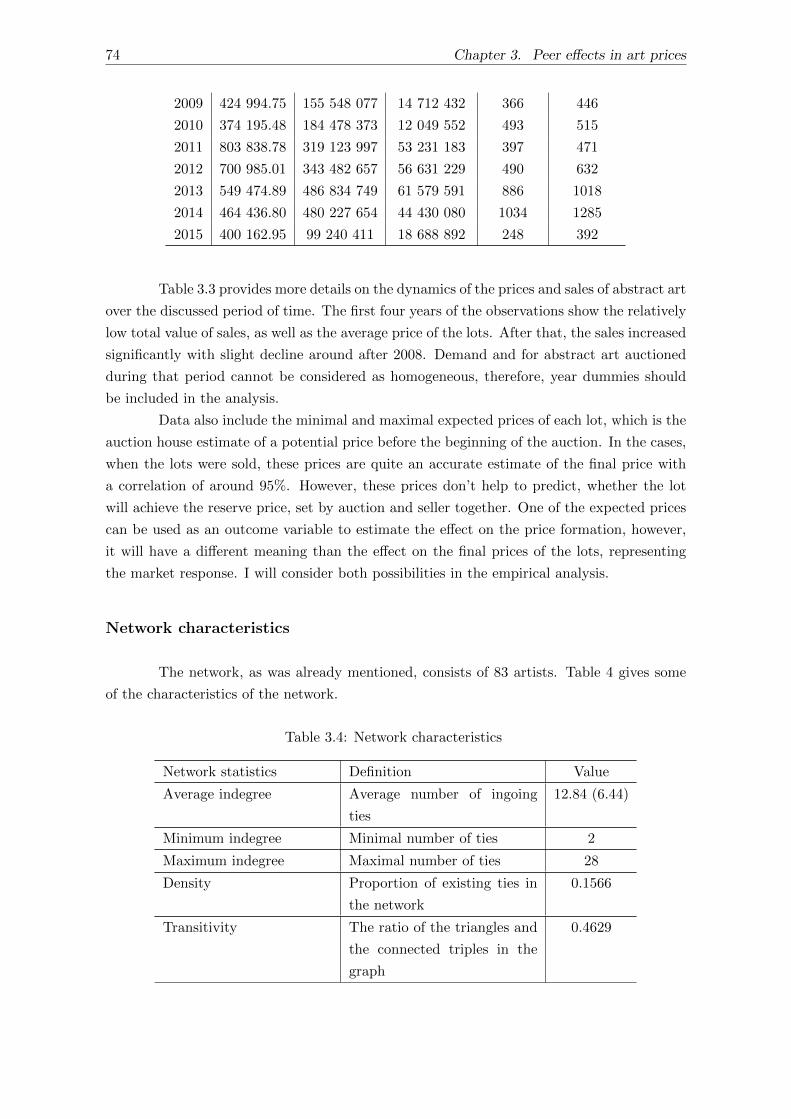
74 Chapter 3. Peer effects in art prices
2009 424 994.75 155 548 077 14 712 432 366 446
2010 374 195.48 184 478 373 12 049 552 493 515
2011 803 838.78 319 123 997 53 231 183 397 471
2012 700 985.01 343 482 657 56 631 229 490 632
2013 549 474.89 486 834 749 61 579 591 886 1018
2014 464 436.80 480 227 654 44 430 080 1034 1285
2015 400 162.95 99 240 411 18 688 892 248 392
Table 3.3 provides more details on the dynamics of the prices and sales of abstract art
over the discussed period of time. The first four years of the observations show the relatively
low total value of sales, as well as the average price of the lots. After that, the sales increased
significantly with slight decline around after 2008. Demand and for abstract art auctioned
during that period cannot be considered as homogeneous, therefore, year dummies should
be included in the analysis.
Data also include the minimal and maximal expected prices of each lot, which is the
auction house estimate of a potential price before the beginning of the auction. In the cases,
when the lots were sold, these prices are quite an accurate estimate of the final price with
a correlation of around 95%. However, these prices don’t help to predict, whether the lot
will achieve the reserve price, set by auction and seller together. One of the expected prices
can be used as an outcome variable to estimate the effect on the price formation, however,
it will have a different meaning than the effect on the final prices of the lots, representing
the market response. I will consider both possibilities in the empirical analysis.
Network characteristics
The network, as was already mentioned, consists of 83 artists. Table 4 gives some
of the characteristics of the network.
Table 3.4: Network characteristics
Network statistics Definition Value
Average indegree Average number of ingoing
ties
12.84 (6.44)
Minimum indegree Minimal number of ties 2
Maximum indegree Maximal number of ties 28
Density Proportion of existing ties in
the network
0.1566
Transitivity The ratio of the triangles and
the connected triples in the
graph
0.4629
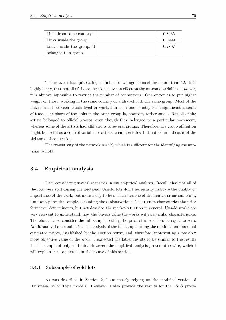
3.4. Empirical analysis 75
Links from same country 0.8435
Links inside the group 0.0999
Links inside the group, if
belonged to a group
0.2807
The network has quite a high number of average connections, more than 12. It is
highly likely, that not all of the connections have an effect on the outcome variables, however,
it is almost impossible to restrict the number of connections. One option is to put higher
weight on those, working in the same country or affiliated with the same group. Most of the
links formed between artists lived or worked in the same country for a significant amount
of time. The share of the links in the same group is, however, rather small. Not all of the
artists belonged to official groups, even though they belonged to a particular movement,
whereas some of the artists had affiliations to several groups. Therefore, the group affiliation
might be useful as a control variable of artists’ characteristics, but not as an indicator of the
tightness of connections.
The transitivity of the network is 46%, which is sufficient for the identifying assump-
tions to hold.
3.4 Empirical analysis
I am considering several scenarios in my empirical analysis. Recall, that not all of
the lots were sold during the auctions. Unsold lots don’t necessarily indicate the quality or
importance of the work, but more likely to be a characteristic of the market situation. First,
I am analysing the sample, excluding these observations. The results characterize the price
formation determinants, but not describe the market situation in general. Unsold works are
very relevant to understand, how the buyers value the works with particular characteristics.
Therefore, I also consider the full sample, letting the price of unsold lots be equal to zero.
Additionally, I am conducting the analysis of the full sample, using the minimal and maximal
estimated prices, established by the auction house, and, therefore, representing a possibly
more objective value of the work. I expected the latter results to be similar to the results
for the sample of only sold lots. However, the empirical analysis proved otherwise, which I
will explain in more details in the course of this section.
3.4.1 Subsample of sold lots
As was described in Section 2, I am mostly relying on the modified version of
Hausman-Taylor Type models. However, I also provide the results for the 2SLS proce-
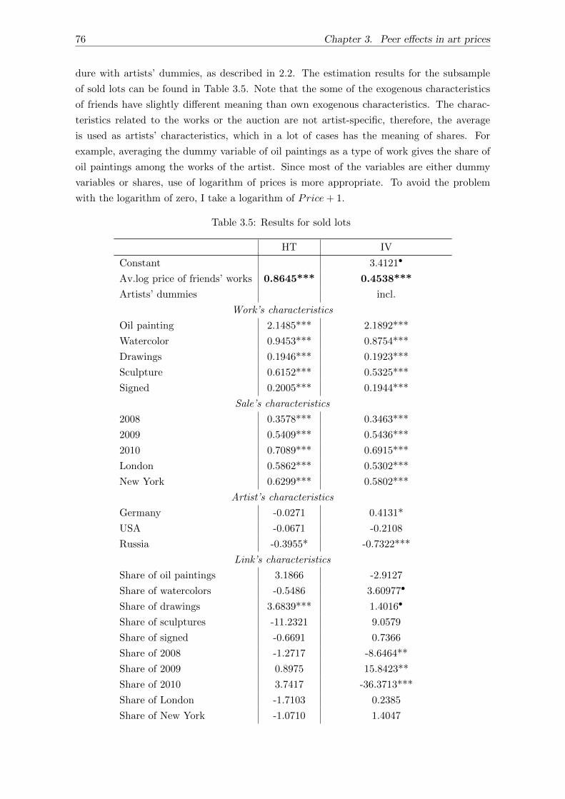
76 Chapter 3. Peer effects in art prices
dure with artists’ dummies, as described in 2.2. The estimation results for the subsample
of sold lots can be found in Table 3.5. Note that the some of the exogenous characteristics
of friends have slightly different meaning than own exogenous characteristics. The charac-
teristics related to the works or the auction are not artist-specific, therefore, the average
is used as artists’ characteristics, which in a lot of cases has the meaning of shares. For
example, averaging the dummy variable of oil paintings as a type of work gives the share of
oil paintings among the works of the artist. Since most of the variables are either dummy
variables or shares, use of logarithm of prices is more appropriate. To avoid the problem
with the logarithm of zero, I take a logarithm of Price+ 1.
Table 3.5: Results for sold lots
HT IV
Constant 3.4121•
Av.log price of friends’ works 0.8645*** 0.4538***
Artists’ dummies incl.
Work’s characteristics
Oil painting 2.1485*** 2.1892***
Watercolor 0.9453*** 0.8754***
Drawings 0.1946*** 0.1923***
Sculpture 0.6152*** 0.5325***
Signed 0.2005*** 0.1944***
Sale’s characteristics
2008 0.3578*** 0.3463***
2009 0.5409*** 0.5436***
2010 0.7089*** 0.6915***
London 0.5862*** 0.5302***
New York 0.6299*** 0.5802***
Artist’s characteristics
Germany -0.0271 0.4131*
USA -0.0671 -0.2108
Russia -0.3955* -0.7322***
Link’s characteristics
Share of oil paintings 3.1866 -2.9127
Share of watercolors -0.5486 3.60977•
Share of drawings 3.6839*** 1.4016•
Share of sculptures -11.2321 9.0579
Share of signed -0.6691 0.7366
Share of 2008 -1.2717 -8.6464**
Share of 2009 0.8975 15.8423**
Share of 2010 3.7417 -36.3713***
Share of London -1.7103 0.2385
Share of New York -1.0710 1.4047
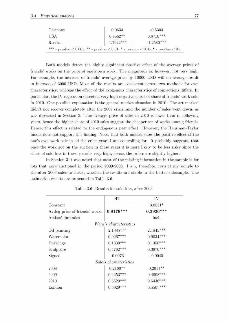
3.4. Empirical analysis 77
Germany 0.0634 -0.5304
USA 0.8562** 0.8710***
Russia -1.7922*** -1.2580***
*** - p-value < 0.001, ** - p-value < 0.01, * - p-value < 0.05, • - p-value < 0.1
Both models detect the highly significant positive effect of the average prices of
friends’ works on the price of one’s own work. The magnitude is, however, not very high.
For example, the increase of friends’ average price by 10000 USD will on average result
in increase of 3000 USD. Most of the results are consistent across two methods for own
characteristics, whereas the effect of the exogenous characteristics of connections differs. In
particular, the IV regression detects a very high negative effect of share of friends’ work sold
in 2010. One possible explanation is the general market situation in 2010. The art marked
didn’t not recover completely after the 2008 crisis, and the number of sales went down, as
was discussed in Section 3. The average price of sales in 2010 is lower than in following
years, hence the higher share of 2010 sales suggest the cheaper set of works among friends.
Hence, this effect is related to the endogenous peer effect. However, the Hausman-Taylor
model does not support this finding. Note, that both models show the positive effect of the
one’s own work sale in all the crisis years I am controlling for. It probably suggests, that
once the work got on the auction in these years it is more likely to be less risky since the
share of sold lots in these years is very high, hence, the prices are slightly higher.
In Section 3 it was noted that most of the missing information in the sample is for
lots that were auctioned in the period 2000-2003. I am, therefore, restrict my sample to
the after 2003 sales to check, whether the results are stable in the better subsample. The
estimation results are presented in Table 3.6.
Table 3.6: Results for sold lots, after 2003
HT IV
Constant 3.8531•
Av.log price of friends’ works 0.8179*** 0.3926***
Artists’ dummies incl.
Work’s characteristics
Oil painting 2.1385*** 2.1845***
Watercolor 0.9267*** 0.9034***
Drawings 0.1339*** 0.1350***
Sculpture 0.4762*** 0.3970***
Signed -0.0073 -0.0045
Sale’s characteristics
2008 0.2160** 0.2011**
2009 0.4253*** 0.4008***
2010 0.5629*** 0.5436***
London 0.5929*** 0.5507***
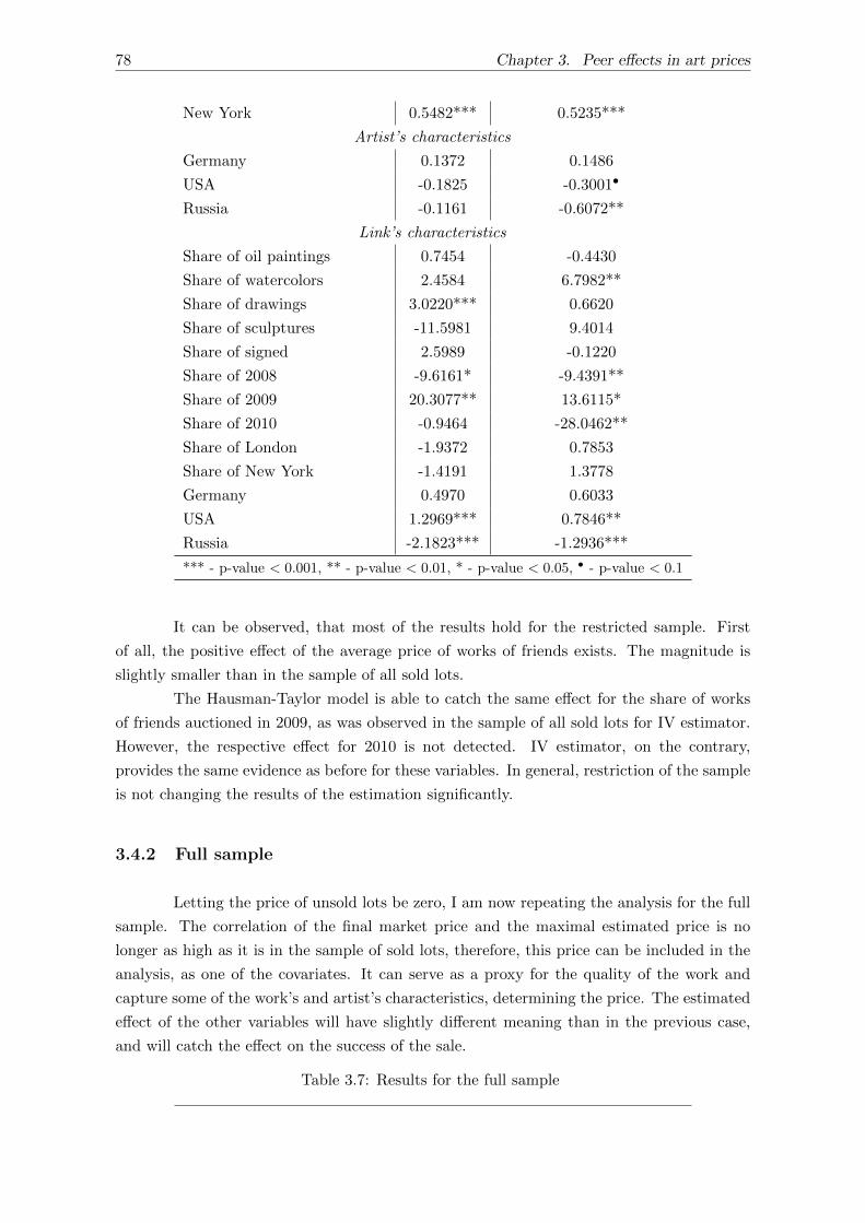
78 Chapter 3. Peer effects in art prices
New York 0.5482*** 0.5235***
Artist’s characteristics
Germany 0.1372 0.1486
USA -0.1825 -0.3001•
Russia -0.1161 -0.6072**
Link’s characteristics
Share of oil paintings 0.7454 -0.4430
Share of watercolors 2.4584 6.7982**
Share of drawings 3.0220*** 0.6620
Share of sculptures -11.5981 9.4014
Share of signed 2.5989 -0.1220
Share of 2008 -9.6161* -9.4391**
Share of 2009 20.3077** 13.6115*
Share of 2010 -0.9464 -28.0462**
Share of London -1.9372 0.7853
Share of New York -1.4191 1.3778
Germany 0.4970 0.6033
USA 1.2969*** 0.7846**
Russia -2.1823*** -1.2936***
*** - p-value < 0.001, ** - p-value < 0.01, * - p-value < 0.05, • - p-value < 0.1
It can be observed, that most of the results hold for the restricted sample. First
of all, the positive effect of the average price of works of friends exists. The magnitude is
slightly smaller than in the sample of all sold lots.
The Hausman-Taylor model is able to catch the same effect for the share of works
of friends auctioned in 2009, as was observed in the sample of all sold lots for IV estimator.
However, the respective effect for 2010 is not detected. IV estimator, on the contrary,
provides the same evidence as before for these variables. In general, restriction of the sample
is not changing the results of the estimation significantly.
3.4.2 Full sample
Letting the price of unsold lots be zero, I am now repeating the analysis for the full
sample. The correlation of the final market price and the maximal estimated price is no
longer as high as it is in the sample of sold lots, therefore, this price can be included in the
analysis, as one of the covariates. It can serve as a proxy for the quality of the work and
capture some of the work’s and artist’s characteristics, determining the price. The estimated
effect of the other variables will have slightly different meaning than in the previous case,
and will catch the effect on the success of the sale.
Table 3.7: Results for the full sample
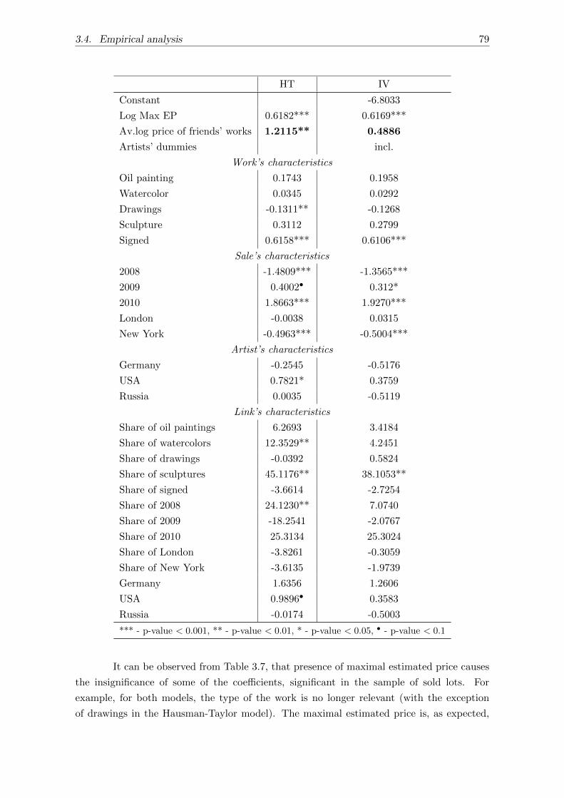
3.4. Empirical analysis 79
HT IV
Constant -6.8033
Log Max EP 0.6182*** 0.6169***
Av.log price of friends’ works 1.2115** 0.4886
Artists’ dummies incl.
Work’s characteristics
Oil painting 0.1743 0.1958
Watercolor 0.0345 0.0292
Drawings -0.1311** -0.1268
Sculpture 0.3112 0.2799
Signed 0.6158*** 0.6106***
Sale’s characteristics
2008 -1.4809*** -1.3565***
2009 0.4002• 0.312*
2010 1.8663*** 1.9270***
London -0.0038 0.0315
New York -0.4963*** -0.5004***
Artist’s characteristics
Germany -0.2545 -0.5176
USA 0.7821* 0.3759
Russia 0.0035 -0.5119
Link’s characteristics
Share of oil paintings 6.2693 3.4184
Share of watercolors 12.3529** 4.2451
Share of drawings -0.0392 0.5824
Share of sculptures 45.1176** 38.1053**
Share of signed -3.6614 -2.7254
Share of 2008 24.1230** 7.0740
Share of 2009 -18.2541 -2.0767
Share of 2010 25.3134 25.3024
Share of London -3.8261 -0.3059
Share of New York -3.6135 -1.9739
Germany 1.6356 1.2606
USA 0.9896• 0.3583
Russia -0.0174 -0.5003
*** - p-value < 0.001, ** - p-value < 0.01, * - p-value < 0.05, • - p-value < 0.1
It can be observed from Table 3.7, that presence of maximal estimated price causes
the insignificance of some of the coefficients, significant in the sample of sold lots. For
example, for both models, the type of the work is no longer relevant (with the exception
of drawings in the Hausman-Taylor model). The maximal estimated price is, as expected,

80 Chapter 3. Peer effects in art prices
highly significant.
The endogenous effect, in which I am mostly interested, is present only in Hausman-
Taylor model analysis. The magnitude is even bigger than in the sample of the sold lots,
suggesting that the average prices of friends’ work might be even more relevant for the
market responses although the two models are different, and the direct comparison of the
coefficient not totally correct. I also run the regressions without maximal estimated price,
which repeats the model from the previous subsection completely. The results are reported
in Table C.3 in Appendix. This model is a worse fit than the one above, and the endogenous
effects are insignificant.
The analysis of the sample of all lots auctioned after 2003 does not detect the
endogenous effect at all, whereas the other results are quite similar to the full sample (see
Table C.2 in Appendix).
3.4.3 Full sample, Maximal and Minimal Estimated Prices
I continue the analysis of the full sample of the lots with the new outcome variable:
estimated by auctioneer price of the lot. The obtained endogenous effect is opposite from
the one obtained for the final market price of sold lots.
Table 3.8: Results for the full sample, max and min EP
HT, Max IV, Max HT, Min
Constant 18.5371***
Av.log price of friends’ works -1.0643*** -0.6299*** -1.0925***
Artists’ dummies incl.
Work’s characteristics
Oil painting 2.1836*** 2.2183*** 2.1838***
Watercolor 0.7829*** 0.7663*** 0.7708***
Drawings 0.2199*** 0.2258*** 0.2227***
Sculpture 0.4816*** 0.4512*** 0.4826***
Signed 0.1162*** 0.1123*** 0.1118**
Sale’s characteristics
2008 0.4195*** 0.3920*** 0.4204***
2009 0.5097*** 0.5069* 0.5125***
2010 0.6793*** 0.6968*** 0.6680***
London 0.5233*** 0.4869*** 0.5203***
New York 0.7845*** 0.7376*** 0.7716***
Artist’s characteristics
Germany 1.0920*** 0.7959*** 1.0947***
USA -0.1613 0.0797 -0.1674
Russia -0.3871* -0.7442*** -0.3933*
Link’s characteristics
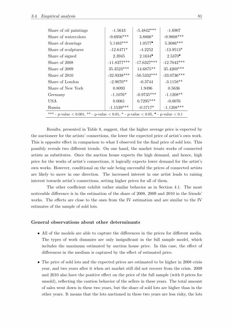
3.4. Empirical analysis 81
Share of oil paintings -1.5643 -5.4842*** -1.6907
Share of watercolors -9.6956*** 3.8806* -9.9808***
Share of drawings 5.1483*** 1.0577• 5.3086***
Share of sculptures -12.6471* -4.2252 -13.9513*
Share of signed 2.3945 2.1634• 2.5370•
Share of 2008 -11.8377*** -17.6327*** -12.7042***
Share of 2009 35.3523*** 14.6875** 35.4269***
Share of 2010 -32.9338*** -50.5332*** -33.0736***
Share of London -2.9070** -0.3744 -3.1158**
Share of New York 0.8093 1.9496 0.5636
Germany -1.1076* -0.9735*** -1.1208**
USA 0.0061 0.7295*** -0.0076
Russia -1.1539*** -0.5717* -1.1208***
*** - p-value < 0.001, ** - p-value < 0.01, * - p-value < 0.05, • - p-value < 0.1
Results, presented in Table 8, suggest, that the higher average price is expected by
the auctioneer for the artists’ connections, the lower the expected price of artist’s own work.
This is opposite effect in comparison to what I observed for the final price of sold lots. This
possibly reveals two different trends. On one hand, the market treats works of connected
artists as substitutes. Once the auction house expects the high demand, and hence, high
price for the works of artist’s connections, it logically expects lower demand for the artist’s
own works. However, conditional on the sale being successful the prices of connected artists
are likely to move in one direction. The increased interest in one artist leads to raising
interest towards artist’s connections, setting higher prices for all of them.
The other coefficient exhibit rather similar behavior as in Section 4.1. The most
noticeable difference is in the estimation of the share of 2008, 2009 and 2010 in the friends’
works. The effects are close to the ones from the IV estimation and are similar to the IV
estimates of the sample of sold lots.
General observations about other determinants
• All of the models are able to capture the differences in the prices for different media.
The types of work dummies are only insignificant in the full sample model, which
includes the maximum estimated by auction house price. In this case, the effect of
differences in the medium is captured by the effect of estimated price.
• The price of sold lots and the expected prices are estimated to be higher in 2008 crisis
year, and two years after it when art market still did not recover from the crisis. 2009
and 2010 also have the positive effect on the price of the full sample (with 0 prices for
unsold), reflecting the caution behavior of the sellers in these years. The total amount
of sales went down in these two years, but the share of sold lots are higher than in the
other years. It means that the lots auctioned in these two years are less risky, the lots
82 Chapter 3. Peer effects in art prices
with less uncertainty about their quality or value, hence ”better” works were auctioned
in these difficult for the market years. The dummy for 2008 for the full sample with
unsold lots exhibits opposite behavior to the one in the sold lot sample. The share
of sold lots in 2008 is very low due to the crisis, therefore, the amount of zero-priced
works is higher in 2008, resulting in the negative highly significant coefficient.
• Sotheby’s London and New York are the main auction locations and attract more
buyers, hence, the more valuable lots are likely to be auctioned there. The price of
sold lots is, therefore, likely to be higher for sales on one of the two locations. Once I
am analysing the sample with unsold lots and including the maximal expected price,
that accounts for a lot of lots characteristics, the prices in New York are likely to be
lower. It reflects the higher probability of having unsold lots, once the volume of sales
is bigger than at the other locations.
• Russian art is very popular in the recent decades7 with every auction house having
their own Russian Art Auction couple of times per year, and ”works by Russian Avant-
Garde are among the most sought-after on the international market” (Hewitt, 2014).
The result of my analysis suggests that the prices of the Russian artists are on average
lower, and being connected to more Russian artists lower the price as well. So the
high demand for Russian art does not result in higher prices in comparison to the
other nationalities. It is reasonable to assume that the affordability and availability of
Russian abstract art is one of the determinants of its high demand.
3.5 Conclusion
This paper adopts the peer effect logic to analyse the price formation on the art
market. I explore the auction results for abstract art from Sotheby’s auction house for the
period of 2000-first half of 2015 and the connections between the abstract artists as reported
for the MOMA exhibition ”Inventing abstraction”. The connections between the artists can
be an important determinant of the artists’ style and quality of works, as well as of the
resulting price of the works. It can be caused by collaborations, joint exhibitions or the
particular reputation of one of the artist’s connections.
I am proposing the model, combining Hausman and Taylor (1981) approach for the
panel data with the Manski(1993) peer effect model and Bramoulle et al. (2009) instru-
ments. I am also using the alternative model, that uses artists’ dummies instead of the panel
structure.
I am analysing both the sample of only sold lots and the full sample setting the price
of unsold lots to zero. Both settings exhibit the positive peer effect of connections’ works
average prices, with more prominent effect in the sold lots sample. The market is, therefore,
rather responsive to the artist’s connections performance and reputations and the buyers are
7See, for example, the report on London Russian Weeks Auction sales

3.5. Conclusion 83
willing to pay more if the artist is connected to the ”better” artist.
The auctioneers behaviour towards price formation is, however, likely to be different.
The more valuable the average works of the connected artists are, the smaller is the expected
minimal and maximal prices set by the auction house before the sales begin. The auction
house probably views the connected artists as substitutes. Moreover, the more ”valuable”
peer group of particular artist suggests that the best artists among the group and the artist
him/herself are probably among the peer group and not the artist. Hence, this artist’s work
are valued lower by the specialists.
The data used in the analysis have several limitations described in Section 3, which
can distort some of the results. However, the paper shows clear evidence of the importance
of connections in the price formation and market outcomes at the art market.
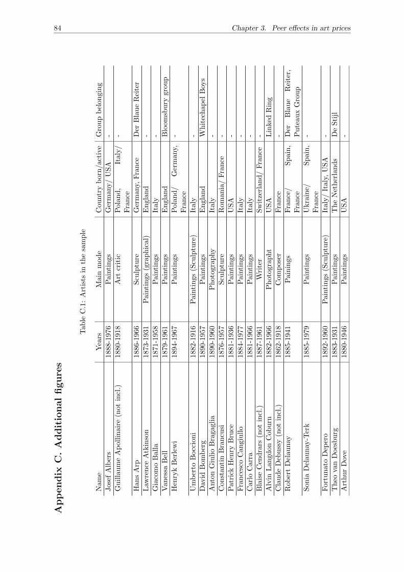
84 Chapter 3. Peer effects in art prices
Ap
pen
dix
C.
Ad
dit
ion
al
figu
res
Tab
leC
.1:
Art
ists
inth
esa
mp
le
Nam
eY
ears
Mai
nm
od
eC
ountr
yb
orn
/act
ive
Gro
up
bel
on
gin
g
Jos
efA
lber
s18
88-1
976
Pai
nti
ngs
Ger
man
y/
US
A-
Gu
illa
um
eA
pol
lin
aire
(not
incl
.)18
80-1
918
Art
crit
icP
olan
d,
Italy
/F
ran
ce-
Han
sA
rp18
86-1
966
Scu
lptu
reG
erm
any,
Fra
nce
Der
Bla
ue
Rei
ter
Law
ren
ceA
tkin
son
1873
-193
1P
ainti
ngs
(gra
phic
al)
En
glan
d-
Gia
com
oB
alla
1871
-195
8P
ainti
ngs
Ital
y-
Van
essa
Bel
l18
79-1
961
Pai
nti
ngs
En
glan
dB
loom
sbu
rygro
up
Hen
ryk
Ber
lew
i18
94-1
967
Pai
nti
ngs
Pol
and
/G
erm
any,
Fra
nce
-
Um
ber
toB
occ
ion
i18
82-1
916
Pai
nti
ngs
(Scu
lptu
re)
Ital
y-
Dav
idB
omb
erg
1890
-195
7P
ainti
ngs
En
glan
dW
hit
ech
ap
elB
oys
Anto
nG
iuli
oB
raga
glia
1890
-196
0P
hot
ogra
phy
Ital
y-
Con
stan
tin
Bra
ncu
si18
76-1
957
Scu
lptu
reR
oman
ia/
Fra
nce
-
Pat
rick
Hen
ryB
ruce
1881
-193
6P
ainti
ngs
US
A-
Fra
nce
sco
Can
giu
llo
1884
-197
7P
ainti
ngs
Ital
y-
Car
loC
arra
1881
-196
6P
ainti
ngs
Ital
y-
Bla
ise
Cen
dra
rs(n
otin
cl.)
1887
-196
1W
rite
rS
wit
zerl
and
/F
ran
ce-
Alv
inL
angd
onC
obu
rn18
82-1
966
Ph
otog
rap
ht
US
AL
inke
dR
ing
Cla
ud
eD
ebu
ssy
(not
incl
.)18
62-1
918
Com
pos
erF
ran
ce-
Rob
ert
Del
aun
ay18
85-1
941
Pai
nin
gsF
ran
ce/
Sp
ain
,F
ran
ceD
erB
lau
eR
eite
r,P
ute
au
xG
rou
p
Son
iaD
elau
nay
-Ter
k18
85-1
979
Pai
nti
ngs
Ukra
ine/
Sp
ain
,F
ran
ce-
For
tun
ato
Dep
ero
1892
-196
0P
ainti
ngs
(Scu
lptu
re)
Ital
y/
Ital
y,U
SA
-
Th
eova
nD
oes
bu
rg18
83-1
931
Pai
nti
ngs
Th
eN
eth
erla
nd
sD
eS
tijl
Art
hu
rD
ove
1880
-194
6P
ainti
ngs
US
A-

3.5. Conclusion 85
Mar
cel
Du
cham
p18
87-1
968
Pai
nti
ngs
(Scu
lptu
re)
Fra
nce
/F
ran
ce,
US
AS
oci
ete
An
onym
e,P
ute
au
xG
rou
p
Su
zan
ne
Du
cham
p18
89-1
963
Pai
nti
ngs
Fra
nce
-
Vik
ing
Egg
elin
g18
80-1
925
Var
iou
sm
edia
Sw
eden
/G
erm
any
Das
Neu
eL
eben
,N
ovem
ber
gru
pp
e
Kse
nii
aE
nd
er18
94-1
955
Pai
nti
ngs
Ru
ssia
-
Hen
riG
aud
ier-
Brz
eska
1891
-191
5S
culp
ture
Fra
nce
/F
ran
ce,
En
glan
d-
Au
gust
oG
iaco
met
ti18
77-1
947
Pai
nti
ngs
Sw
itze
rlan
d/
Sw
itze
rlan
d,
Italy
-
Nat
alia
Gon
char
ova
1881
-196
2P
ainti
ngs
Ru
ssia
/R
uss
ia,
Fra
nce
Pu
teau
xG
rou
p,
Don
key’s
Tail
Du
nca
nG
rant
1885
-197
8P
ainti
ngs
En
glan
dB
loom
sbu
ryG
rou
p
Mar
sden
Har
tley
1877
-194
3P
ainti
ngs
US
A/
US
A,
Ger
-m
any
-
Vil
mos
Hu
szar
1884
-196
0P
ainti
ngs
Hu
nga
ry/
Th
eN
eth
erla
nd
sD
eS
tijl
Vas
ily
Kan
din
sky
1866
-194
4P
ainti
ngs
Ru
ssia
/R
uss
ia,
Ger
-m
any
Der
Bla
ue
Rei
ter
Pau
lK
lee
1879
-194
0P
ainti
ngs
Sw
itze
rlan
d/
Ger
-m
any,
Sw
itze
rlan
dD
erB
lau
eR
eite
r
Ivan
Kli
un
1873
-194
3S
culp
ture
Ru
ssia
Un
ion
of
You
th,
Su
pre
mu
s
Gu
stav
Klu
tsis
1895
-193
8P
hot
ogra
phy
Lat
via
/L
atvia
,R
us-
sia
-
Kat
arzy
na
Kob
ro18
98-1
951
Scu
lptu
reR
uss
ia/
Ru
ssia
,P
olan
d-
Ale
kse
iK
ruch
enykh
(not
incl
.)18
86-1
968
Poet
Ru
ssia
-
Fra
nti
sek
Ku
pka
1871
-195
7P
ainti
ngs
(Gra
ph
ics)
Cze
chR
epu
bli
c/F
ran
ceP
ute
au
xG
rou
p
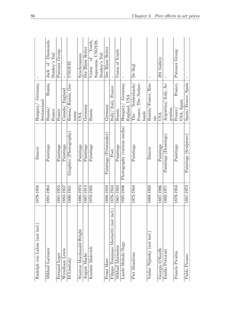
86 Chapter 3. Peer effects in art prices
Ru
dol
ph
von
Lab
an(n
otin
cl.)
1879
-195
8D
ance
rH
un
gary
/G
erm
any,
Sw
itze
rlan
d-
Mik
hai
lL
ario
nov
1881
-196
4P
ainti
ngs
Ru
ssia
/R
uss
ia,
Fra
nce
Jack
of
Dia
mon
ds,
Don
key’s
Tail
Fer
nan
dL
eger
1881
-195
5P
ainti
ngs
Fra
nce
Pu
teau
xG
rou
p
Wyn
dh
amL
ewis
1882
-195
7P
ainti
ngs
Can
ada/
En
glan
d-
El
Lis
sitz
ky
1890
-194
1G
rap
hic
s(P
hot
ogra
phy)
Ru
ssia
/R
uss
ia,
Ger
-m
any
UN
OV
IS
Sta
nto
nM
acd
onal
d-W
righ
t18
90-1
973
Pai
nti
ngs
US
AS
yn
chro
mis
m
Au
gust
Mac
ke18
87-1
914
Pai
nti
ngs
Ger
man
yD
erB
lau
eR
eite
r
Kaz
imir
Mal
evic
h18
78-1
935
Pai
nti
ngs
Ru
ssia
Un
ion
of
You
th,
Su
pre
mu
s,U
NO
VIS
,D
on
key’s
Tail
Fra
nz
Mar
c18
80-1
916
Pai
nti
ngs
(Pri
ntm
aker
)G
erm
any
Der
Bla
ue
Rei
ter
Fil
ipp
oT
omm
aso
Mar
inet
ti(n
otin
cl.)
1876
-194
4P
oet
Ital
y/
Ital
y,F
ran
ce-
Mik
hai
lM
atiu
shin
1861
-193
4P
ainti
ngs
Ru
ssia
Un
ion
of
You
th
Las
zlo
Moh
oly-N
agy
1895
-194
6P
hot
ogra
phy
(var
iou
sm
edia
)H
un
gary
/G
erm
any,
En
glan
d,
US
A-
Pie
tM
ond
rian
1972
-194
4P
ainti
ngs
Th
eN
eth
erla
nd
s/F
ran
ce,
Th
eN
eth
er-
lan
ds
De
Sti
jl
Vas
lav
Nij
insk
y(n
otin
cl.)
1889
-195
0D
ance
rR
uss
ia/
Fra
nce
,R
us-
sia
-
Geo
rgia
O’K
eeff
e18
87-1
986
Pai
nti
ngs
US
A291
Gall
ery
Em
ilio
Pet
toru
ti18
92-1
971
Pai
nti
ngs
(Dra
win
gs)
Arg
enti
na/
Ital
y,A
r-ge
nti
na
-
Fra
nci
sP
icab
ia18
79-1
953
Pai
nti
ngs
Fra
nce
/F
ran
ce,
US
A,
Sp
ain
Pu
teau
xG
rou
p
Pab
loP
icas
so18
81-1
973
Pai
nti
ngs
(Scu
lptu
re)
Sp
ain
/F
ran
ce,S
pain
-

3.5. Conclusion 87
Liu
bov
Pop
ova
1889
-192
4P
ainti
ngs
Ru
ssia
/R
uss
ia,
Fra
nce
Kn
ave
of
Dia
mon
ds,
Su
pre
mu
s
Man
Ray
1890
-197
6P
hot
ogra
phy
(Var
iou
sm
edia
)U
SA
/U
SA
,F
ran
ce-
Han
sR
ichte
r18
88-1
976
Pai
nti
ngs
(Fil
mm
aker
)G
erm
any/
Ger
many,
Sw
itze
rlan
d,
US
AA
rtis
tes
Rad
icau
x
Ale
ksa
nd
rR
od
chen
ko18
91-1
956
Ph
otog
rap
hy
(Scu
lptu
re)
Ru
ssia
Oct
ob
erC
ircl
e
Mor
gan
Ru
ssel
1886
-195
3P
ainti
ngs
US
A/
US
A,
Fra
nce
Syn
chro
mis
m
Lu
igi
Ru
ssol
o18
85-1
947
Pai
nti
ngs
(Com
pos
er)
Ital
y/
Ital
y,A
r-ge
nti
na
-
Hel
enS
aun
der
s18
85-1
963
Pai
nti
ngs
En
glan
d-
Ch
rist
ian
Sch
ad18
94-1
982
Pai
nti
ngs
Ger
man
y/
Ger
many,
Sw
itze
rlan
d,
Italy
-
Mor
ton
Liv
ings
ton
Sch
amb
erg
1881
-191
8P
ainti
ngs
(Ph
otog
rap
hy)
US
AS
oci
ete
An
onym
e
Arn
old
Sch
oen
ber
g(n
otin
cl.)
1874
-195
1C
omp
oser
Au
stri
a/G
erm
any
Der
Bla
ue
Rei
ter
Ku
rtS
chw
itte
rs18
87-1
948
Var
iou
sm
edia
Ger
man
y-
Gin
oS
ever
ini
1883
-196
6P
ainti
ngs
Ital
y/
Ital
y,F
ran
ce-
Ard
engo
Soffi
ci18
79-1
964
Pai
nti
ngs
(Wri
ter)
Ital
y/
Ital
y,F
ran
ce-
Jos
eph
Ste
lla
1877
-194
6P
ainti
ngs
Ital
y/
US
A,
Fra
nce
,It
aly
-
Alf
red
Sti
egli
tz18
64-1
946
Ph
otog
rap
hy
US
A291
Gall
ery
Pau
lS
tran
d18
90-1
976
Ph
otog
rap
hy
US
A291
Gall
ery
Wla
dysl
awStr
zem
insk
i18
93-1
953
Pai
nti
ngs
Pol
and
/R
uss
iaB
lok
Leo
pol
dS
urv
age
1879
-196
8P
ainti
ngs
Ru
ssia
/F
ran
ce-
Wac
law
Szp
akow
ski
1883
-197
3G
rap
hic
sP
olan
d-
Sop
hie
Tae
ub
er-A
rp18
89-1
943
Pai
nti
ngs
(Gra
ph
ics)
Sw
itze
rlan
dC
ercl
eel
Carr
e
Vla
dim
irT
atli
n18
85-1
953
Pai
nti
ngs
(Arc
hit
ectu
re)
Ru
ssia
Un
ion
of
You
th
Tri
stan
Tza
ra(n
otin
cl.)
1896
-196
3P
oet
Rom
ania
/R
oman
ia,
Sw
itze
rlan
d,
Fra
nce
-
Geo
rges
Van
ton
gerl
oo
1886
-196
5S
culp
ture
Bel
giu
m/
Th
eN
eth
erla
nd
s,F
ran
ceD
eS
tijl

88 Chapter 3. Peer effects in art prices
Ed
gar
Var
ese
(not
incl
.)18
83-1
965
Com
pos
erF
ran
ce/
Ger
many,
US
A-
Max
Web
er18
81-1
961
Pai
nti
ngs
Ru
ssia
/U
SA
-
Mar
yW
igm
an(n
otin
cl.)
1886
-197
3D
ance
rG
erm
any/
Ger
many,
Sw
itze
rlan
d-
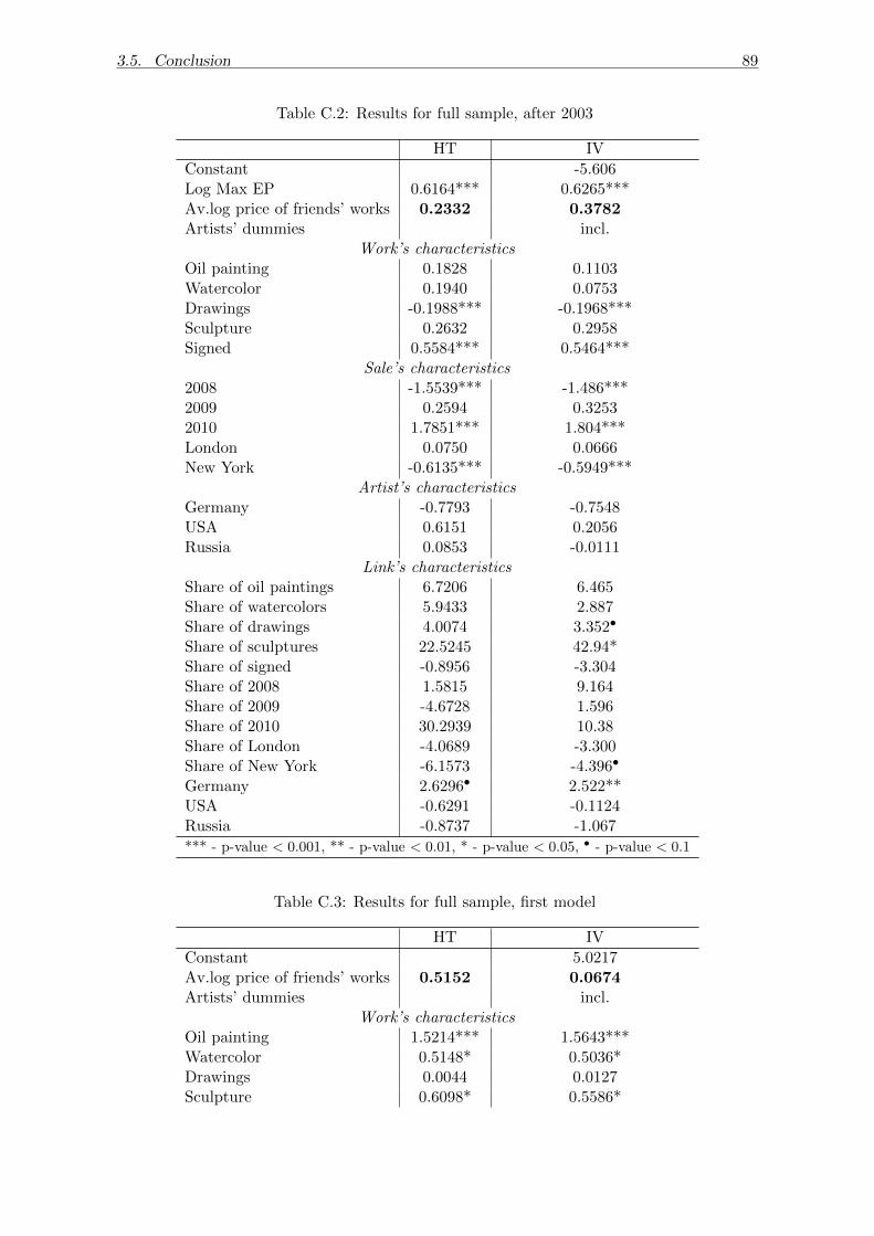
3.5. Conclusion 89
Table C.2: Results for full sample, after 2003
HT IV
Constant -5.606Log Max EP 0.6164*** 0.6265***Av.log price of friends’ works 0.2332 0.3782Artists’ dummies incl.
Work’s characteristicsOil painting 0.1828 0.1103Watercolor 0.1940 0.0753Drawings -0.1988*** -0.1968***Sculpture 0.2632 0.2958Signed 0.5584*** 0.5464***
Sale’s characteristics2008 -1.5539*** -1.486***2009 0.2594 0.32532010 1.7851*** 1.804***London 0.0750 0.0666New York -0.6135*** -0.5949***
Artist’s characteristicsGermany -0.7793 -0.7548USA 0.6151 0.2056Russia 0.0853 -0.0111
Link’s characteristicsShare of oil paintings 6.7206 6.465Share of watercolors 5.9433 2.887Share of drawings 4.0074 3.352•
Share of sculptures 22.5245 42.94*Share of signed -0.8956 -3.304Share of 2008 1.5815 9.164Share of 2009 -4.6728 1.596Share of 2010 30.2939 10.38Share of London -4.0689 -3.300Share of New York -6.1573 -4.396•
Germany 2.6296• 2.522**USA -0.6291 -0.1124Russia -0.8737 -1.067
*** - p-value < 0.001, ** - p-value < 0.01, * - p-value < 0.05, • - p-value < 0.1
Table C.3: Results for full sample, first model
HT IV
Constant 5.0217Av.log price of friends’ works 0.5152 0.0674Artists’ dummies incl.
Work’s characteristicsOil painting 1.5214*** 1.5643***Watercolor 0.5148* 0.5036*Drawings 0.0044 0.0127Sculpture 0.6098* 0.5586*
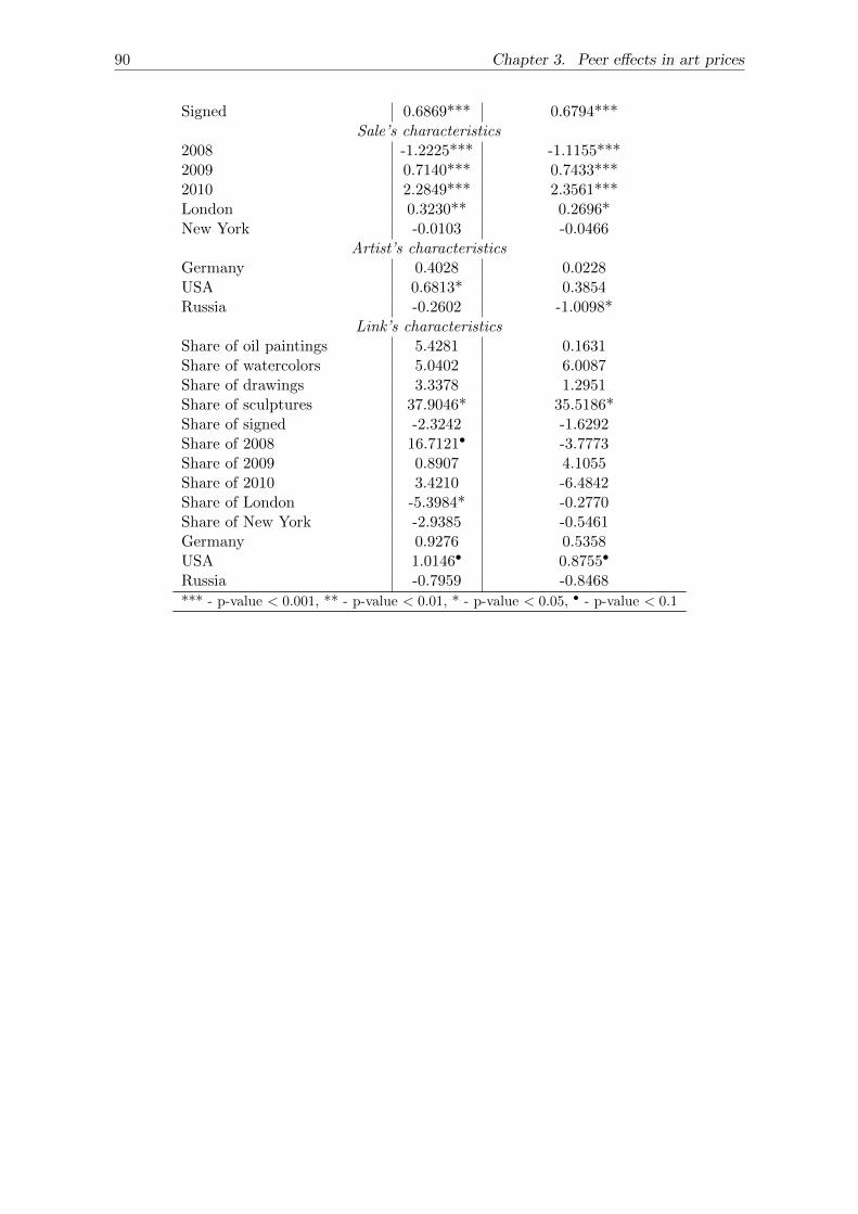
90 Chapter 3. Peer effects in art prices
Signed 0.6869*** 0.6794***Sale’s characteristics
2008 -1.2225*** -1.1155***2009 0.7140*** 0.7433***2010 2.2849*** 2.3561***London 0.3230** 0.2696*New York -0.0103 -0.0466
Artist’s characteristicsGermany 0.4028 0.0228USA 0.6813* 0.3854Russia -0.2602 -1.0098*
Link’s characteristicsShare of oil paintings 5.4281 0.1631Share of watercolors 5.0402 6.0087Share of drawings 3.3378 1.2951Share of sculptures 37.9046* 35.5186*Share of signed -2.3242 -1.6292Share of 2008 16.7121• -3.7773Share of 2009 0.8907 4.1055Share of 2010 3.4210 -6.4842Share of London -5.3984* -0.2770Share of New York -2.9385 -0.5461Germany 0.9276 0.5358USA 1.0146• 0.8755•
Russia -0.7959 -0.8468
*** - p-value < 0.001, ** - p-value < 0.01, * - p-value < 0.05, • - p-value < 0.1

References, chapter 3
Ashenfelter, Orley (1989). “How auctions work for wine and art”. In: The Journal of Eco-nomic Perspectives 3.3, pp. 23–36.
Ashenfelter, Orley and Kathryn Graddy (2003). “Auctions and the price of art”. In: Journalof Economic Literature 41.3, pp. 763–787.
— (2006). “Art auctions”. In: Handbook of the Economics of Art and Culture 1, pp. 909–945.Auction results at Sotheby’s. url: http://www.sothebys.com/en.html.Banksy (2010). ”Exit through the Gift Shop”. Movie.Baumol, William J (1986). “Unnatural value: or art investment as floating crap game”. In:
The American Economic Review 76.2, pp. 10–14.Capgemini (2013). World Wealth Report. url: https://www.worldwealthreport.com/
download/68/b95e0b47.Chilvers, Ian (2003). A dictionary of twentieth-century art. Oxford University Press.Consumer Price Index Data. url: http://www.usinflationcalculator.com/inflation/
consumer-price-index-and-annual-percent-changes-from-1913-to-2008/.Global art sales in 2014 break all known records (2015). url: http://www.tefaf.com/
DesktopDefault.aspx?tabid=15&pressrelease=16959&presslanguage.Goetzmann, William N (1993). “Accounting for taste: Art and the financial markets over
three centuries”. In: The American Economic Review 83.5, pp. 1370–1376.Goetzmann, William N, Luc Renneboog, and Christophe Spaenjers (2011). “Art and money”.
In: The American Economic Review 101.3, pp. 222–226.Hausman, Jerry A and William E Taylor (1981). “Panel data and unobservable individual
effects”. In: Econometrica, pp. 1377–1398.Hewitt, Simon (2014). London’s Russian Auction Market. Russian Art Week Analysis 2007-
2014. url: http://www.russianartweek.co.uk/wp-content/uploads/2012/10/Russian-Art-Market-Report-by-Simon-Hewitt-Nov14.pdf.
Horowitz, Noah (2014). Art of the deal: Contemporary art in a global financial market. Prince-ton University Press.
Inventing Abstraction at MOMA. url: http://www.moma.org/interactives/exhibitions/2012/inventingabstraction/.
Journal, Wall Street (2010). “Follow your heart?” In: The Wall Street Journal Europe, TheJournal Report: Wealth Adviser September 20.
Kleiner, Fred S. (2015). Gardner’s Art through the Ages: A Global History. Cengage.McAndrew, Clare (2010). The International Art Market 2007-2009: Trends in the Art Trade
during Global Recession. European Fine Art Foundation (TEFAF).Mei, Jianping and Michael Moses (2002). “Art as an investment and the underperformance
of masterpieces”. In: The American Economic Review 92.5, pp. 1656–1668.Renneboog, Luc and Christophe Spaenjers (2013). “Buying beauty: On prices and returns
in the art market”. In: Management Science 59.1, pp. 36–53.
91

92 REFERENCES, CHAPTER 3
Representative Exchange Rates. url: http://www.imf.org/external/np/fin/data/
param_rms_mth.aspx.Sagot-Duvauroux, Dominique (2003). “Art prices”. In: A Handbook of Cultural Economics,
p. 57.Shirley, Andrew (2014). Knight Frank Luxury Investment Index update 2014. url: http://
www.knightfrankblog.com/wealthreport/news-headlines/knight-frank-luxury-
investment-index-update-2014/.Thompson, Don (2010). The $12 million stuffed shark: The curious economics of contempo-
rary art. Macmillan.

Full Bibliography
Ammermueller, A. and J.-S. Pischke (2009). “Peer effects in European primary schools:Evidence from the progress in international reading literacy study”. In: Journal of LaborEconomics 27.3, pp. 315–348.
Androushchak, Gregory, Oleg Poldin, and Maria Yudkevich (2013). “Role of peers in studentacademic achievement in exogenously formed university groups”. In: Educational Studies39.5, pp. 568–581.
Angrist, J.D. and K. Lang (2004). “Does school integration generate peer effects? Evidencefrom Boston’s Metco Program”. In: American Economic Review, pp. 1613–1634.
Aral, S., L. Muchnik, and A. Sundararajan (2009). “Distinguishing influence-based contagionfrom homophily-driven diffusion in dynamic networks”. In: Proceedings of the NationalAcademy of Sciences 106.51, pp. 21544–21549.
Ashenfelter, Orley (1989). “How auctions work for wine and art”. In: The Journal of Eco-nomic Perspectives 3.3, pp. 23–36.
Ashenfelter, Orley and Kathryn Graddy (2003). “Auctions and the price of art”. In: Journalof Economic Literature 41.3, pp. 763–787.
— (2006). “Art auctions”. In: Handbook of the Economics of Art and Culture 1, pp. 909–945.Auction results at Sotheby’s. url: http://www.sothebys.com/en.html.AUSTRALIA: High drop-out rates cost $1.4 billion (2010). url: http://www.universityworldnews.
com/article.php?story=20101022203542738.Banksy (2010). ”Exit through the Gift Shop”. Movie.Battin-Pearson, S. et al. (2000). “Predictors of early high school dropout: A test of five
theories.” In: Journal of educational psychology 92.3, pp. 568–582.Baumol, William J (1986). “Unnatural value: or art investment as floating crap game”. In:
The American Economic Review 76.2, pp. 10–14.Belloni, Alexandre, Victor Chernozhukov, and Ivan Fernandez-Val (2011). “Conditional
quantile processes based on series or many regressors”. In:Bramoulle, Y., H. Djebbari, and B. Fortin (2009). “Identification of peer effects through
social networks”. In: Journal of econometrics 150.1, pp. 41–55.Buchmann, Claudia and Ben Dalton (2002). “Interpersonal influences and educational aspira-
tions in 12 countries: The importance of institutional context”. In: Sociology of education75, pp. 99–122.
Calvo-Armengol, A., E. Patacchini, and Y. Zenou (2009). “Peer effects and social networksin education”. In: The Review of Economic Studies 76.4, pp. 1239–1267.
Capgemini (2013). World Wealth Report. url: https://www.worldwealthreport.com/download/68/b95e0b47.
Carrell, S.E., R.L. Fullerton, and J.E. West (2009). “Does your cohort matter? Measuringpeer effects in college achievement”. In: Journal of Labor Economics 27.3, pp. 439–464.
Chandrasekhar, A. and R. Lewis (2011). “Econometrics of sampled networks”. In: Unpub-lished manuscript, MIT.[422].
93

94 FULL BIBLIOGRAPHY
Chaudhuri, Probal (1991). “Nonparametric estimates of regression quantiles and their localBahadur representation”. In: The Annals of statistics 19.2, pp. 760–777.
Chaudhuri, Probal, Kjell Doksum, and Alexander Samarov (1997). “On average derivativequantile regression”. In: The Annals of Statistics 25.2, pp. 715–744.
Chilvers, Ian (2003). A dictionary of twentieth-century art. Oxford University Press.Coleman, J.S. (1990). Foundations of social theory. Harvard university press.Comola, M. and S. Prina (2014). “Do interventions change the network? A dynamic peer
effect model accounting for network changes”. In: Working paper.Consumer Price Index Data. url: http://www.usinflationcalculator.com/inflation/
consumer-price-index-and-annual-percent-changes-from-1913-to-2008/.De Giorgi, Giacomo, Michele Pellizzari, and Silvia Redaelli (2010). “Identification of social
interactions through partially overlapping peer groups”. In: American Economic Journal:Applied Economics, pp. 241–275.
Dette, Holger and Stanislav Volgushev (2008). “Non-crossing non-parametric estimates ofquantile curves”. In: Journal of the Royal Statistical Society: Series B (Statistical Method-ology) 70.3, pp. 609–627.
El Ghouch, Anouar and Ingrid Van Keilegom (2009). “Local linear quantile regression withdependent censored data”. In: Statistica Sinica, pp. 1621–1640.
Elhorst, J. Paul (2010). “Dynamic panels with endogenous interaction effects when T issmall”. In: Regional Science and Urban Economics 40.5, pp. 272–282.
French, D.C. and J. Conrad (2001). “School dropout as predicted by peer rejection andantisocial behavior”. In: Journal of Research on adolescence 11.3, pp. 225–244.
Gardner, Michael (2007). GERMANY: Heavy cost of student drop-outs. url: http://www.universityworldnews.com/article.php?story=20071025102357719.
Garnier, H.E., J.A. Stein, and J.K. Jacobs (1997). “The process of dropping out of highschool: A 19-year perspective”. In: American Educational Research Journal 34.2, pp. 395–419.
Gaviria, A. and S. Raphael (2001). “School-based peer effects and juvenile behavior”. In:Review of Economics and Statistics 83.2, pp. 257–268.
Global art sales in 2014 break all known records (2015). url: http://www.tefaf.com/DesktopDefault.aspx?tabid=15&pressrelease=16959&presslanguage.
Goetzmann, William N (1993). “Accounting for taste: Art and the financial markets overthree centuries”. In: The American Economic Review 83.5, pp. 1370–1376.
Goetzmann, William N, Luc Renneboog, and Christophe Spaenjers (2011). “Art and money”.In: The American Economic Review 101.3, pp. 222–226.
Goldsmith-Pinkham, P. and Guido W Imbens (2013). “Social networks and the identificationof peer effects”. In: Journal of Business & Economic Statistics 31.3, pp. 253–264.
Guerre, Emmanuel and Camille Sabbah (2012). “Uniform bias study and Bahadur represen-tation for local polynomial estimators of the conditional quantile function”. In: Econo-metric Theory 28.01, pp. 87–129.
Hanushek, E.A. et al. (2003). “Does peer ability affect student achievement?” In: Journal ofapplied econometrics 18.5, pp. 527–544.
Hardle, Wolfgang and Thomas M Stoker (1989). “Investigating smooth multiple regressionby the method of average derivatives”. In: Journal of the American Statistical Association84.408, pp. 986–995.
Hausman, Jerry A and William E Taylor (1981). “Panel data and unobservable individualeffects”. In: Econometrica, pp. 1377–1398.
He, Xuming and Pin Ng (1999). “Quantile splines with several covariates”. In: Journal ofStatistical Planning and Inference 75.2, pp. 343–352.

FULL BIBLIOGRAPHY 95
He, Xuming, Pin Ng, and Stephen Portnoy (1998). “Bivariate quantile smoothing splines”. In:Journal of the Royal Statistical Society: Series B (Statistical Methodology) 60.3, pp. 537–550.
Hewitt, Simon (2014). London’s Russian Auction Market. Russian Art Week Analysis 2007-2014. url: http://www.russianartweek.co.uk/wp-content/uploads/2012/10/Russian-Art-Market-Report-by-Simon-Hewitt-Nov14.pdf.
Hoderlein, Stefan and Enno Mammen (2009). “Identification and estimation of local aver-age derivatives in non-separable models without monotonicity”. In: The EconometricsJournal 12.1, pp. 1–25.
Hong, Sheng-Yan (2003). “Bahadur representation and its applications for local polynomialestimates in nonparametric M-regression”. In: Journal of Nonparametric Statistics 15.2,pp. 237–251.
Horowitz, Noah (2014). Art of the deal: Contemporary art in a global financial market. Prince-ton University Press.
Hoxby, C. (2000). Peer effects in the classroom: Learning from gender and race variation.Tech. rep. National Bureau of Economic Research.
Indicators of economics of education, url: https://memo.hse.ru/ind.Inventing Abstraction at MOMA. url: http://www.moma.org/interactives/exhibitions/
2012/inventingabstraction/.Jackson, Matthew O. (2010). “An overview of social networks and economic applications”.
In: The handbook of social economics 1, pp. 511–585.Journal, Wall Street (2010). “Follow your heart?” In: The Wall Street Journal Europe, The
Journal Report: Wealth Adviser September 20.Kelejian, Harry H and Ingmar R Prucha (1998). “A generalized spatial two-stage least
squares procedure for estimating a spatial autoregressive model with autoregressive dis-turbances”. In: The Journal of Real Estate Finance and Economics 17.1, pp. 99–121.
Kleiner, Fred S. (2015). Gardner’s Art through the Ages: A Global History. Cengage.Koenker, Roger (2005). Quantile regression. Cambridge university press.Koenker, Roger and Gilbert Bassett Jr (1978). “Regression quantiles”. In: Econometrica:
journal of the Econometric Society, pp. 33–50.Koenker, Roger, Pin Ng, and Stephen Portnoy (1994). “Quantile smoothing splines”. In:
Biometrika 81.4, pp. 673–680.Kong, Efang, Oliver Linton, and Yingcun Xia (2010). “Uniform Bahadur representation for
local polynomial estimates of M-regression and its application to the additive model”.In: Econometric Theory 26.05, pp. 1529–1564.
Lee, Lungfei (2003). “Best Spatial Two-Stage Least Squares Estimators for a Spatial Au-toregressive Model with Autoregressive Disturbances”. In: Econometric Reviews 22.4,pp. 307–335.
Lee, Young Kyung and Eun Ryung Lee (2008). “Kernel methods for estimating derivativesof conditional quantiles”. In: Journal of the Korean Statistical Society 37.4, pp. 365–373.
Li, Qi and Jeffrey S Racine (2008). “Nonparametric estimation of conditional CDF andquantile functions with mixed categorical and continuous data”. In: Journal of Business& Economic Statistics 26.4, pp. 423–434.
Lomi, A. et al. (2011). “Why are some more peer than others? Evidence from a longitudi-nal study of social networks and individual academic performance”. In: Social ScienceResearch 40.6, pp. 1506–1520.
Mammen, Enno, Ingrid Van Keilegom, and Kyusang Yu (2015). “Expansion for moments ofregression quantiles with application to nonparametric testing”. In: Working Paper.
Manski, C.F. (1993). “Identification of endogenous social effects: The reflection problem”.In: The review of economic studies 60.3, pp. 531–542.

96 FULL BIBLIOGRAPHY
McAndrew, Clare (2010). The International Art Market 2007-2009: Trends in the Art Tradeduring Global Recession. European Fine Art Foundation (TEFAF).
McPherson, M., L. Smith-Lovin, and J. M. Cook (2001). “Birds of a feather: Homophily insocial networks”. In: Annual review of sociology, pp. 415–444.
Mei, Jianping and Michael Moses (2002). “Art as an investment and the underperformanceof masterpieces”. In: The American Economic Review 92.5, pp. 1656–1668.
Metco program official webpage. url: http://www.doe.mass.edu/metco/.Newcomb, M.D. (1996a). “Adolescence: Pathologizing a normal process.” In: The counseling
Psychologist 24, pp. 482–490.— (1996b). “Pseudomaturity among adolescents: Construct validation, sex differences, and
associations in adulthood.” In: Journal of Drug Issues 26, pp. 477–504.Paula, Aureo de (2015). “Econometrics of Network Models”. In: cemmap Working paper
CWP52/15.Poldin, Oleg, Diliara Valeeva, and Maria Yudkevich (2015). “Which Peers Matter: How Social
Ties Affect Peer-group Effects”. In: Research in Higher Education, pp. 1–21.Portnoy, Stephen (1997). “Local asymptotics for quantile smoothing splines”. In: The Annals
of Statistics, pp. 414–434.Renneboog, Luc and Christophe Spaenjers (2013). “Buying beauty: On prices and returns
in the art market”. In: Management Science 59.1, pp. 36–53.Representative Exchange Rates. url: http://www.imf.org/external/np/fin/data/
param_rms_mth.aspx.Roy, Arati et al. (1976). “The structure of degraded bael (Aegle marmelos) gum”. In: Car-
bohydrate Research 50.1, pp. 87–96.Rumberger, R.W. (1983). “Dropping out of high school: The influence of race, sex, and family
background”. In: American Educational Research Journal.Sacerdote, B. (2011). “Peer effects in education: How might they work, how big are they
and how much do we know thus far?” In: Handbook of the Economics of Education 3,pp. 249–277.
Sacerdote, Bruce (2001). “Peer Effects with Random Assignment: Results for DartmouthRoommates”. In: Quartetly Journal of Economics 116.2, pp. 681–704.
Sagot-Duvauroux, Dominique (2003). “Art prices”. In: A Handbook of Cultural Economics,p. 57.
Shirley, Andrew (2014). Knight Frank Luxury Investment Index update 2014. url: http://www.knightfrankblog.com/wealthreport/news-headlines/knight-frank-luxury-
investment-index-update-2014/.Shugal, N. (2010). “Potoki obuchayushchikhsya v rossiyskoy sisteme obrazovaniya [Student
flows in Russian education system]”. In: Voprosy obrazovaniya / Educational Studies 4,pp. 122–148.
Smith, J.P. and R.A. Naylor (2001). “Dropping Out of University: A Statistical Analysisof the Probability of Withdrawal for UK University Students”. In: Journal of the RoyalStatistical Society. Series A (Statistics in Society) 164.2, pp. 389–405.
Socio-Economic situation in Russia (2014). url: http://www.gks.ru/bgd/regl/b14_01/Main.htm.
Stinebrickner, T. and R. Stinebrickner (2013). Academic performance and college dropout:Using longitudinal expectations data to estimate a learning model. Tech. rep. NationalBureau of Economic Research.
Thompson, Don (2010). The $12 million stuffed shark: The curious economics of contempo-rary art. Macmillan.
Tinto, V. (1975). “Dropout from higher education: A theoretical synthesis of recent research”.In: Review of educational research, pp. 89–125.

FULL BIBLIOGRAPHY 97
Triandis, Harry C (1989). “The self and social behavior in differing cultural contexts.” In:Psychological review 96.3, pp. 506–520.