ECONOMETRIC ANALYSIS OF FISHER’S EQUATION BY PETER...

ECONOMETRIC ANALYSIS OF FISHER’S EQUATION

BY

PETER C.B. PHILLIPS

COWLES FOUNDATION PAPER NO. 1173

COWLES FOUNDATION FOR RESEARCH IN ECONOMICS YALE UNIVERSITY

Box 208281 New Haven, Connecticut 06520-8281

2006

http://cowles.econ.yale.edu/

Econometric Analysis of Fisher’s Equation

By PETER C. B. PHILLIPS*

ABSTRACT. Fisher’s equation for the determination of the real rate ofinterest is studied from a fresh econometric perspective. Some newmethods of data description for nonstationary time series are intro-duced. The methods provide a nonparametric mechanism for mod-elling the spatial densities of a time series that displays randomwandering characteristics, like interest rates and inflation. Hazard ratefunctionals are also constructed, an asymptotic theory is given, andthe techniques are illustrated in some empirical applications to realinterest rates for the United States. The paper ends by calculatingsemiparametric estimates of long-range dependence in U.S. real inter-est rates, using a new estimation procedure called modified log periodogram regression and new asymptotics that covers the nonsta-tionary case. The empirical results indicate that the real rate of inter-est in the United States is (fractionally) nonstationary over 1934–1997and over the more recent subperiods 1961–1985 and 1961–1997. Unitroot nonstationarity and short memory stationarity are both stronglyrejected for all these periods.

I

Introduction

SINCE IRVING FISHER (1896, 1930) formalized1 the notion of a real rateof interest, the concept has played a significant role in the formula-tion of a wide range of economic models. These include individualagent decision making regarding investment, savings, and portfolioallocations, options pricing models in finance, and the modern theoryof inflation targeting in macroeconomics, to name but a few. Natu-rally enough, in light of the role that the real rate plays in economictheory models, a good deal of attention has been devoted in the lit-erature, especially in macroeconomics, to the measurement of the real

The American Journal of Economics and Sociology, Vol. 64, No. 1 ( January, 2005).© 2005 American Journal of Economics and Sociology, Inc.

*Peter C. B. Phillips is a professor of economics and statistics at Yale University and

the editor of Econometric Theory.

rate and to the characterization of its temporal dependence proper-ties. Prima facie, this task seems like a simple exercise in time serieseconometrics. However, the empirical analysis is complicated by two factors: (1) the apparent nonstationary behavior of the seriesinvolved, particularly interest rates but also sometimes inflation; and(2) the fact that the ex ante real rate of interest depends on inflationexpectations and is therefore not directly measured. Perhaps becauseof these complicating factors, no consensus seems to have emergedabout the time series properties of the real rate of interest, in spiteof intensive empirical study. In particular, while economic theorymodels routinely assume that the real rate of interest is a constant, orfluctuates in a stationary way about a constant mean, the empiricalwork indicates that this is not so or at best holds only over shortregimes.

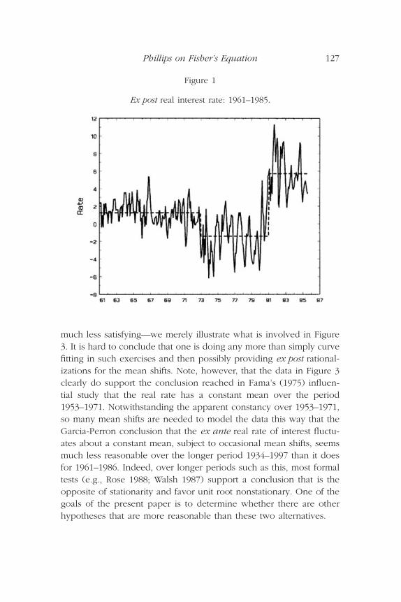
Figure 1 shows monthly data for the ex post real interest rate in theUnited States over the period 1961:1–1985:12. The series is calculatedby taking the U.S. 90-day treasury bill rate for the nominal interestrate and by using the U.S. monthly CPI (all commodities, with noadjustment for housing costs) to compute three-month inflation rates.The figure also shows subgroup means calculated over the subperi-ods 1961:1–1973:1, 1973:2–1982:1, and 1982:2–1985:12. The datacover the same period as that studied recently by Garcia and Perron(1994), who used regime shift methods to estimate the ex ante realrate over approximately these subperiods. These authors concludedthat the ex ante real rate of interest was effectively constant but subjectto occasional mean shifts over 1961–1985. They found two mean shiftsover this time period and gave results very similar to those obtainedby subgroup means that are displayed in Figure 1. For these data, atleast, the conclusion does not seem unreasonable.

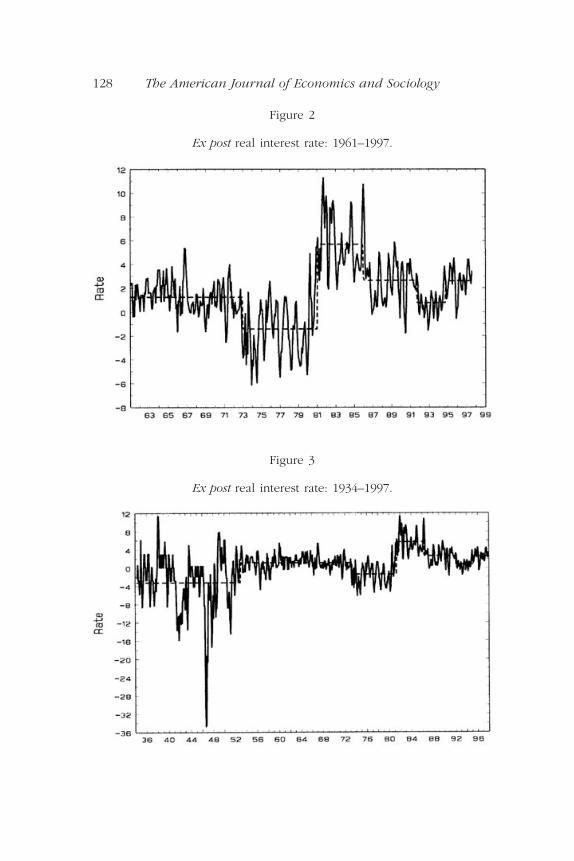
Figures 2 and 3 graph the ex post real interest rate series calculatedin the same way over the longer periods 1961–1997 and 1934–1997.Over the 1961–1997 period the graphs shows subsample means forthe additional two subperiods 1990–1993 and 1994–1997. Apparently,there is a need to allow for continuing regime shifts in the mean levelif this approach to modeling the real rate of interest is to give accept-able results. For the longer period, an even larger number of meanshifts is needed to accommodate this approach, and the results seem

126 The American Journal of Economics and Sociology

Phillips on Fisher’s Equation 127

Figure 1

Ex post real interest rate: 1961–1985.

much less satisfying—we merely illustrate what is involved in Figure3. It is hard to conclude that one is doing any more than simply curvefitting in such exercises and then possibly providing ex post rational-izations for the mean shifts. Note, however, that the data in Figure 3clearly do support the conclusion reached in Fama’s (1975) influen-tial study that the real rate has a constant mean over the period1953–1971. Notwithstanding the apparent constancy over 1953–1971,so many mean shifts are needed to model the data this way that theGarcia-Perron conclusion that the ex ante real rate of interest fluctu-ates about a constant mean, subject to occasional mean shifts, seemsmuch less reasonable over the longer period 1934–1997 than it doesfor 1961–1986. Indeed, over longer periods such as this, most formaltests (e.g., Rose 1988; Walsh 1987) support a conclusion that is theopposite of stationarity and favor unit root nonstationary. One of thegoals of the present paper is to determine whether there are otherhypotheses that are more reasonable than these two alternatives.


Figure 3


Figure 2


Another goal of the paper is to contribute some new methods toassist in the econometric analysis of data of this type. The methodsgiven here furnish a new way of describing and characterizing datalike interest rates and inflation that appear to have nonstationary ele-ments. More specifically, the paper proposes a nonparametric spatialdensity estimate as a new descriptive tool for nonstationary timeseries. Many series like the interest rates shown in Figures 1–3 behaveas if they have no fixed mean. The random wandering characteristicof these series is hard to describe quantitatively. What a spatial densitydoes is provide useful quantitative information about the spatial loca-tion characteristics of a time series, in just the same way as a prob-ability density can be used to characterize stationary time series. Aswill be shown, in contrast to a probability density, the spatial densityis a random process. However, it turns out that we can still obtainconsistent estimates of spatial densities using nonparametric tech-niques, like those of kernel methods, which have proved useful instudying iid and strictly stationary time series. We outline these newprocedures here and provide an asymptotic theory that characterizestheir large sample properties and facilitates inference.

Once nonparametric spatial density estimates have been obtained,we can use them in similar ways to that of a probability density—tostudy and quantify the locational characteristics of the time series. Weillustrate these ideas by looking at nonparametric estimates of thespatial location of the ex post real rate of interest in the United States.This exercise provides some nonparametric evidence on recent empir-ical findings about real interest rates and the Fisher effect. In addi-tion, we show how to construct a new type of hazard function fornonstationary time series. Hazard rates are particularly helpful instudying financial series, as they can be used to quantify the hazardsof certain interest rate and inflation rate levels, for example. Themethods can also be used to study how empirical hazard rates evolveover time. Again, we illustrate the techniques in some empirical appli-cations to the ex post real rate of interest series for the U.S. economyshown in Figures 1–3.

Finally, we attempt to model the real rate of interest directly as apotentially nonstationary long memory process. This involves theeconometric estimation of the long memory parameter (d ), without


making any delimiting assumptions about the short memory com-ponents in the data generating process. The procedure we use is anew semiparametric estimator developed by the author (1999a) inrecent work on fractional processes. This new estimator is called modified log periodogram (LP) regression. Kim and Phillips (1999a)have shown that, in contrast to log periodogram regression, thismethod has good asymptotic properties for values of d over the fullregion 0 < d < 2, so that it is well suited for use with time series,like interest rates, whose memory parameters may extend into thenonstationary region where

We will briefly describe the new approach in Section VI and use themethod to estimate d and to provide confidence intervals, therebyenabling us to answer the question of whether the preferred modelfor data on the real rate of interest is stationary or nonstationary.

The paper is organized as follows. The Fisher effect and associatedregression equations are discussed in Section II. The econometric ideasthat underlie the spatial modeling apparatus that we introduce are laidout in Sections III and IV. Section V provides an empirical applicationof the methods to U.S. data over the period 1934–1997. Section VIreports our new asymptotics and empirical estimates of the longmemory parameter. Section VII concludes the paper and discussessome related issues. Proofs are collected together in Section VIII withsome of the new asymptotic theory that is introduced in the paper.

II

The Fisher Effect

IRVING FISHER FORMULATED THE CONCEPT of the (ex ante) real rate of inter-est ( ) to provide a rate of interest that accounted for the value ofloan repayments in real dollar terms. That is, a nominal interest rateof it will assure a real rate of when the anticipated price changeis provided it = + + , thereby adjusting the compensa-tion to the lender for the anticipated losses in purchasing power inthe principal and the interest. The term is usually ignoredbecause it is of smaller order, so that the Fisher equation is commonlywritten as

p ter t

e

p ter t

ep ter t

ep te

r te

r te

d ≥1

2.


(1)

Equation (1) is sometimes made more specific by indexing the inter-est rate by the time period (m) of the bond to maturity and by usingm-period ahead inflation expectations, leading to the alternate formulation

(2)

The empirical literature surrounding Equation (1) is vast and we will not attempt to provide a review here. Fisher himself beganthe empirical work and considered the problems surrounding the relationship between prices and interest rates to be “of such vitalimportance that I have gone to much trouble and expense to havesuch data as could be found compiled, compared, and analyzed”(1930: p.399).

The main object of Fisher’s work was “to ascertain to what extent, if at all, a change in the general price level actually affects themarket rates of interest” (1930: p.399). He conducted correlationalstudies between inflation and interest rates with annual data prima-rily for the United States and the United Kingdom, concluding asfollows:

Our first correlations seemed to indicate that the relationship between P’(inflation) and i (interest rate) is either very slight or obscured by otherfactors. But when we make the much more reasonable supposition thatprice changes do not exhaust their effects in a single year but manifesttheir influence with diminishing intensity over long periods which vary inlength with the conditions, we find a very significant relationship, espe-cially in the period which includes the World War, when prices weresubject to violent fluctuations. (1930: 423)

Since this initial work by Fisher, a substantial amount of empiricalwork has been conducted with data from many countries, coveringdifferent periods of time and maturities. However, little consensusseems to have emerged from these studies about the nature of theFisher effect. In particular, there seems to be little agreement aboutthe statistical properties of the real rate .

Two recent studies that make significant methodological departuresin studying this problem are by Mishkin (1992) and the already citedpaper by Garcia and Perron (1994). These papers bring some modernnonstationary time series and regime shift methods to bear in

r te

i rtm

te m

te m= +, , .p

i rt te

te= + p .


analyzing the Fisher equation. Using residual-based co-integrationtests, Mishkin finds support in the data for a “long-run” Fisher effectin which inflation and interest rates share a common stochastic trend.Observe that if is the m-period inflation rate, then Equation (2)gives the following relation between the ex post real rate of interest ( ) and the ex ante rate of interest :

(3)

Under rational expectations, where agents or the market use all information efficiently in forecasting inflation, the forecast error et = will be a martingale difference and can be assumed to be stationary, or integrated of order zero (I(0)). Under this hypoth-esis, the ex post and ex ante real rates differ by a stationary compo-nent and therefore have the same long-run time series properties.Thus, following Mishkin (1992), the ex post real rate can only be I(1)if is I(1). Hence, a test for a unit root in against stationaryalternatives can be interpreted as a test for a unit root in againsta stationary ex ante real rate. Put another way, co-integration between

and is the alternative hypothesis in a test for a unit root in the ex post real rate of interest. The Fisher effect then corresponds tothe hypothesis that the ex ante real rate of interest is stationary, sothat, under rational expectations and stationary forecast errors forinflation, the Fisher effect implies a stationary ex post real rate of interest.

In spite of their apparent simplicity, Equations (1) and (3) presenta host of econometric difficulties arising from the fact that the vari-ables and are unmeasured latent variables, and from the timeseries difficulties in modeling apparently nonstationary series likeinterest rates and inflation.

While Fisher (1930) analyzed the relationship between interest ratesand inflation using correlational techniques, modern approaches relyon regression methods—sometimes, as in Summers (1983), in the fre-quency domain where low frequencies can be used to emphasizelong-run properties. Depending on the properties of the real rate

, Equation (3) suggests a regression link between it and . In par-ticular, the Fisher effect asserts that the coefficient b should be unityin a regression of the form

p ter t

e

p ter t

e

p tmi t

m

rte m,

r tmrt

e m,

p pte m

tm, -

r r rtm

te m

te m

tm

te m

t= + -( ) = +, , , .p p e

rte m,r it

mtm

tm= - p

p tm


and the residuals ut should be stationary. Under this hypothesis, wecan write the ex post real rate of interest as

(4)

which implies stationary fluctuations about a constant level c.In a celebrated study mentioned earlier, Fama (1975) found empir-

ical evidence of a constant real rate of interest over the period1953–1971. Mishkin (1981) subsequently rejected constancy in the realrate in a more extensive study covering the longer periods 1953–1979and 1931–1952. Later investigations by Rose (1988) and Walsh (1987)found evidence in support of unit root nonstationarity in ex post realrates. Most recently, Garcia and Perron (1996) reanalyzed data overthe period 1961–1986 using regime shift techniques and foundsupport for a constant real rate of interest, subject to infrequentchanges in the constant c. In short, the empirical evidence gives amixed picture about the statistical properties of the real rate of inter-est, and it is probably fair to say that the generating mechanism forthe real rate is very imperfectly understood. Although the bulk of theeconometric evidence now points against the hypothesis of a pureFisher effect in which the real rate is stationary about a constant mean,this does not rule out modified Fisher effects such as those supportedin the Garcia-Perron study.

We now propose to take a very different approach to studying thesedata. The essence of the new approach is descriptive, but the asymp-totic theory that we have developed for the quantities involvedenables us to use them in an inferential framework as well. This helpsus to corroborate and assess earlier empirical findings.

III

Spatial Densities for Nonstationary Series

OUR PROPOSAL IS TO STUDY the spatial characteristics of a time seriesrather than focus on their temporal dependence properties, as one would normally do in a stationary time series analysis. The starting point is to assume that, when appropriately normalized and

r i c b u c wt t t te

t t t= - = + -( ) + = +p p p ,

i c b ut te

t= + +p


transformed into a random function on the interval [0, 1], the timeseries trajectories converge weakly to those of a continuous stochas-tic process on the same interval. Such an assumption applies undera very wide variety of possible conditions, and it seems a very weakrequirement if one is to make any headway in the development ofasymptotic methods. Accordingly, we may suppose that the limitprocess, M(r), say, of the normalized series is a continuous semi-martingale (see, e.g., Protter 1990). This requirement would theninclude the huge class of time series for which functional central limittheorems are known to apply, leading, for example, to Brownianmotions and diffusion processes as special cases (see, e.g., Phillipsand Solo 1992). While this class of time series is substantial, one casethat is excluded by the semi-martingale requirement is time series thatupon normalization tend to fractional processes like fractional Brown-ian motion (e.g., Mandlebrot and van Ness 1968; Taqqu 1975). Thiscase does seem to be important in applications of our ideas to non-stationary series, because there is increasing evidence that economictime series are well modeled by long memory processes with frac-tional Brownian motion limits; for some recent macroeconomic timeseries evidence, see Gil-Alana and Robinson (1997) and Kim andPhillips (1999a). Fortunately, it seems that it will be possible to includefractional processes within our theory and, although this is not donehere, some discussion and references are provided later (see the para-graph following Equation (12)).

For a semi-martingale M(r) it is known that there exists an increas-ing stochastic process2 (increasing in the argument r, that is) calledthe local time of M at s and denoted LM(r, s) that represents theamount of time that the limit process spends in the spatial vicinity ofthe point s. The local time process is defined as

(5)

where [M ]t is the quadratic variation process of M. Notice that thisdefinition of “time spent in the vicinity of s” is expressed in units ofvariation, as measured by d [M ]t. In effect, LM(r, s) measures the con-tribution to the quadratic variation [M]r over the interval [0, r ] thatcomes from variation in M(t) around the level s.

L r s M t s d MM

r

t, lim ,( ) = ( ) - <( ) [ ]Æ Úe e

e0 0

1

21


It turns out that we can also write down an inverse relation of theform

(6)

which gives a decomposition of the quadratic variation into contri-butions to the conditional variance that come from fluctuations in theprocess that occur in the neighborhood of different spatial points sŒ [-•, •]. In a sense, we can think of Equation (6) as the spatialequivalent for a continuous nonstationary random process of thedecomposition of the variation of a stationary time series into contri-butions from different frequencies, that is,

where fx(l) is the spectral density of Xt and s 2 = var Xt. In this formula,l is a continuous variable representing the frequency of the oscilla-tions into which the time series variation is being decomposed.However, in Equation (6), the variable s represents spatial points inthe real line, where the process spends some time. Fluctuations in the process around the point s, which can occur at various timesin the time interval [0, t ], then contribute to the density LM(t, s) of theprocess at this spatial point.

Equation (6) is particularly interesting in the special case whereM(r) is the Brownian motion B(r) with variance w 2. Here, the param-eter w 2 arises as the long-run variance of the shocks which drive theunit root process that converges weakly to B(r). In this case, we have

giving a decomposition of the long-run variance w 2 into componentsthat reflect the density of the fluctuations in the process around allspatial points s Œ (-•, •).

The local time process LM(r, s) is known to satisfy the followingequation

(7)M r s M s M t s dM t L r sr

M( ) - = ( ) - + ( ) -( ) ( ) + ( )Ú00sgn , ,

w 2 1= ( )-•

•

Ú L s dsB , ,

s l lp

p2 = ( )

-Ú f dxx ,

M L t s dst M[ ] = ( )-•

•

Ú , ,


where sgn(x) = 1, -1 for x > 0, x £ 0. In fact, the process LM(r, s) is sometimes defined in this manner; for example, see Revuz and Yor (1994). Equation (7), gives a development of the function |M(r) - s| is about its value at r = 0 and thereby provides a mech-anism of generalizing the Ito stochastic calculus of functions that arecontinuously differentiable to the second order (C2 functions) to func-tions that are not everywhere differentiable and smooth, and, in particular, to convex functions, which we will show below. Theseextensions look to be particularly valuable in theoretical modelswhere convex functions play a big role, but have not to my knowl-edge been used yet in economic analysis.

As is well known (e.g., Protter 1990: 74), if f Œ C2 we have the Itoformula for continuous semi-martingales given by

(8)

On the other hand, when f is convex we have, based on Equation (7),

(9)

where is the left derivative of f and is the second derivativeof f in the generalized function sense. When f Œ C2 we have (M(t))= f ¢(M(t)), and (p) = f ≤(p), the second derivative in the usual sense,and the occupation time formula (e.g., Revuz and Yor 1991: 209) gives

(10)

so that Equation (9) reduces to Equation (8) in this special case.Observe that Equation (10) shows the sense in which LM(r, p) is a

spatial density for the process M(r), recording the amount of time(measured in units of the quadratic variation [M ]t) that the process hasspent in the immediate vicinity of p over the time interval t Œ [0, r ].

We now propose to use these concepts in studying the spatial prop-erties of time series like interest rates and inflation. Our first task isto estimate the local time process LM(r, p) for a particular time series.Just as the spectral density of a stationary time series is estimated by nonparametric methods, the local time LM(r, p) can be estimated

1

2

1

2 0¢¢( ) ( ) = ¢¢ ( )( ) [ ]

-•

•

Ú Úf p L r p dp f M t d MM t

r, ,

¢¢f g

¢f _

¢¢f g¢f _

f M r f M f M t dM t f p L r p dpr

g M( )( ) = ( )( ) + ¢ ( )( ) ( ) + ¢¢( ) ( )Ú Ú-•

•0

1

20_ , ,

f M r f M f M t dM t f M t d Mr

t

r( )( ) = ( )( ) + ¢ ( )( ) ( ) + ¢¢ ( )( ) [ ]Ú Ú0

1

20 0.


in a nonparametric manner as follows. Let Xt be a time series thatsatisfies a functional law of the form

(11)

where M(r) is a continuous semi-martingale for r Œ [0, 1]. For instance,when Xt is an integrated process of order 1, standard functional centrallimit theorems (e.g., Phillips and Solo 1992) lead to Equation (11)with

a Brownian motion with variance

When Xt is near integrated, so that the quasi differences

are stationary with positive spectral density at the origin, then

a linear diffusion process (e.g., Phillips 1987). On the other hand, whenXt is a fractionally integrated process whose memory parameter

whose initialization is at t = 0, and for which the differenced process(1 - L)d Xt = ut is stationary with positive spectrum w 2 > 0 at theorigin, then we have the following functional law (cf. Akonom andGourieroux 1987)

where Bd-1(r) is a fractional Brownian motion. In this case, the limitprocess M(r) = Bd-1(r) is not a semi-martingale and, indeed, theprocess Bd-1 actually has infinite quadratic variation. Hence, in placeof Equation (5), where quadratic variation is being distributed spa-tially, it is more helpful to define local time according to

11

2

11

0

n

X B rd

r s dW sd

nr ddr

-[ ] -

-fi ( ) =( )

-( ) ( )Úw

G,

d ŒÊË

˘˚

1

21, ,

a = ( ) = ( )1

2and M r J rc ,

D c t t tX Xc

nX= - +Ê

Ëˆ¯ -1 1

w p2 2 0= ( )f xD .

a = ( ) = ( )1

2and M r B r ,

1

nX M rnra [ ] fi ( ),


(12)

which measures the amount of time in chronological units that Mt

spends in the vicinity of s over the interval [0, r]. Accordingly, (r, s) is called the chronological local time of M at s over [0, r ] (cf

Phillips and Park 1998). Local time for the fractional process Bd-1 canbe defined using Equation (12), and Tyurin and Phillips (1999) givea development of the theory of local time using this approach anddiscuss its empirical estimation.

These examples seem to cover most cases of empirical interest thatarise in the present literature on nonstationary economic time series.In the development that follows we will assume we are working withan integrated process Xt for which

Or, if we want to allow for distant initial conditions (at time -[nk ] forsome k ≥ 0) in the origination of Xt then we can use the limit

where B and B0 are independent Brownian motions, with the processB0 extending in a reverse (negative) direction reflecting the effect ofdistant initial conditions at some fraction k of the sample size n. Thiswill cover a wide class of interesting practical cases. Extensions ofthe theory to the more general case of Equation (11) are also possi-ble but are more difficult and will call upon strong approximationversions of Equation (11) that, at least to the author’s present knowl-edge, do not seem to be available in the probability literature as yetfor a general class of processes (although a strong approximation fordiffusion processes is given in Phillips 1998). A complete develop-ment of the asymptotic theory in our case to cover situations asgeneral as Equation (11) is beyond the scope of the present paper.Extensions to the important fractional Brownian motion case are con-sidered by Tyurin and Phillips (1999).

A natural candidate for estimating the local time of the limit process of

at s is the scaled kernel estimate

n X nr

-[ ]

1

2

n X B r Bnr

-[ ] fi ( ) + ( )

1

20 k ,

n X B rnr

-[ ] fi ( )

1

2 .

L M

L r s M t s dtM

r, lim ,( ) = ( ) - <( )

Æ Úe ee

0 0

1

21


(13)

where hn is a bandwidth parameter, K(·) is a symmetric kernel func-tion, and 2 is a consistent estimate of w2 = 2pfDx(0). Upon restandard-ization of this estimate we have the following extension of a resultobtained recently in Phillips and Park (1998).

A. Theorem

Suppose 2 Æp w2 = 2pfDx(0). If s = s0 + a, with s0 and a fixed, andif assumptions VIII.A–VIII.D in the Appendix hold, then as n Æ •

(14)

The definition of

involves scaling the conventional kernel estimator given in Equation(13) by . The reason for this restandardization is that in the non-stationary case the process Xt wanders away from the location s atthe rate and, for such departures from s, K( (s - Xt)) is negli-gibly small. In effect, the stochastic trend property of Xt reduces theorder of magnitude of the kernel estimate compared with the sta-tionary case.

Note that the estimate

evaluates the local time at a spatial point

that is affected by the rate of convergence of

to its Brownian motion limit process. Hence, if s is fixed and initialconditions are Op(1), i.e., k = 0 as n Æ •, then the estimate

is consistent for the local time of the limit process at the origin, thatis, LB(r, 0). When k > 0, the random initialization shifts the spatial

ˆ ,L r n sB-Ê

Ëˆ¯

1

2

n X nr

-[ ]

1

2

n s-

1

2

ˆ ,L r n sB-Ê

Ëˆ¯

1

2

hn-1n

n

ˆ ,L r n sB-Ê

Ëˆ¯

1

2

ˆ ,ˆ

, .L rs

n nhK

s X

hL r a BB

n t

nrt

np B

ÊË

ˆ¯ =

-ÊË

ˆ¯ Æ - ( )( )

=

[ ]

Âwk

2

10

nw

w

ˆ ˆ, ,

w w2

1

2

1nhK

s X

h nhK c

s

n

X

nc

n

hn t

nt

n n t

n

nt

nn= =

Â Â-ÊË

ˆ¯ = -ÏÌÓ

¸˛

ÊË

ˆ¯ =


point of evaluation of the local time estimate so that it is centeredaround B0(k). So, initial conditions generally play a role in the spatialdensity of the process, as we might well expect for a nonstationaryseries.

Our next step is to construct confidence regions for the densityestimate

This can be done using the limiting distribution theory for

given in Theorem III.B below. The limit distribution turns out to bemixed normal (denoted MN in what follows) with a mixing variatethat is proportional to the spatial density itself. This limit theory jus-tifies the construction of confidence intervals in the usual manner.

B. Theorem

If s = s0 + a, with s0 and a fixed, if assumptions VIII.A–VIII.D inthe Appendix hold, and if ( 2 - w 2) = op(1) where cn = ,then as n Æ •

where Q(a, b) is a standard Brownian sheet, W(p) is a standardBrownian motion, and

This result enables us to construct confidence intervals for LB(r, a - B0(k)) for each spatial point. Thus,

ˆ , .

ˆ ,L r n s

K L r n s

cB

B

n

-

-

ÊË

ˆ¯ ±

ÊË

ˆ¯

Ê

Ë

ÁÁÁ

ˆ

¯

˜˜˜

1

2

2

1

2

1

2

1 968

K K p p t K t dpdt200

= ( ) Ÿ( ) ( )••

ÚÚ .

c L r n s L r a B

K p Q L r a B p dp

MN K L r a B

n B B

B

B

ˆ , ,

, ,

, , ,

-

-•

•

ÊË

ˆ¯ - - ( )( )È

ÎÍ˘˚

fi ( ) - ( )( )( )∫ - ( )( )( )

Ú

1

20

0

2 0

2

0 8

k

k

k

nhn-1wcn

n

ˆ ,L r n sB-Ê

Ëˆ¯

1

2

ˆ , .L r n sB-Ê

Ëˆ¯

1

2


is a 95% confidence interval for LB(r, a - B0(k)). When K(·) is a normalkernel, some calculations show that K2 takes the value

Note that we are measuring spatial departures from the origin inunits of in the limit. So, if we want a confidence interval for the spatial density of the process at a point like a0, we set s = a0 + X0 and compute

(15)

It is interesting to compare local time confidence intervals likeEquation (15) above with the confidence intervals for a probabilitydensity from kernel estimates of a probability density. By traditionaltheory here (e.g., Silverman 1986) we have the following 95% confi-dence interval for a density f(x),

(16)

where

(17)

The differences between Equations (15) and (16) involve: (1) the scalefactors k2 and 8K2, where the difference is due to the temporaldependence in the trajectory of Xt (so that the covariance kernelenters the definition of K2) and definitional differences between localtime and a probability density; and (2) the rate of convergence in the case of the spatial density, compared with in the case ofthe probability density. In other respects, Equation (15) simplyextends our existing theory of nonparametric density estimation tospatial density estimation for stochastic processes.

nh- cn

k K r dr22= ( )

-•

•

Ú .

ˆ .ˆ

f xk f x

nh( ) ±

( )ÊËÁ

ˆ¯

1 96 2

1

2

ˆ , .

ˆ ,.L r a n X

K L r a n X

cB

B

n

01

20

20

1

20

1

2

1 968

+ÊË

ˆ¯ ±

+ÊË

ˆ¯

Ê

Ë

ÁÁÁ

ˆ

¯

˜˜˜

-

-

nn

n

K 2

1

2 2 11

2= -ÊËÁ

ˆ¯

-p .


IV

Hazard Rates for Nonstationary Time Series

ONE ADVANTAGE OF A NONPARAMETRIC TREATMENT of spatial density is thatwe can define interesting functionals derived from the density thathelp us to shed light on the nature of variation in the data. Whilethere are many obvious notions that arise in this way, one that wewill pay attention to here is the idea of a spatial hazard function. Wedefine the spatial hazard function HM(t, a) associated with a givenspatial density LM(t, s) as follows:

(18)

The form of Equation (18) is analogous to that of the hazard rate q(x)associated with a probability density f (x) as

where F(x) is the cdf of the distribution and (x) = 1 - F(x) is thesurvivor function. Such conventional hazard rates are now extensivelyused in empirical econometric work to help model and understandphenomena like unemployment duration and quits in the labor marketand have widespread use in other fields, such as the statistical analy-sis of medical phenomena relating to the contraction of diseases.

How do we interpret such hazard rates in the case of nonstation-ary time series? Suppose the time series under study Xt is inflationand M(r) is the weak limit process of n-aX[nr ], with local time LM(r, s).The spatial hazard

measures the conditional risk over the period [0, t] (which isexpressed in standardized units of fractions of the overall sample) ofan inflation rate of s, given that inflation is at least as great as s. Wecan then study the form of this hazard as a function of the inflationrate s, just as we might look at unemployment duration in the con-ventional hazard analysis of independent data. Thus, we can seewhether the hazard declines, increases, or stays constant as we

H t as

nM , =Ê

Ëˆ¯a

F

q xf x

f s ds

f x

F x

f x

F xx

( ) =( )

( )=

( )- ( )

=( )( )•

Ú 1,

H t aL t a

L t s dsM

M

Ma

,,

,.( ) =

( )( )

•

Ú


increase s. We can also look at the hazard as a function of the lengthof the time interval t and examine what happens to the hazard rateas the time period evolves and new data are introduced. So, we cansee whether the hazard rate of a certain rate of inflation rises or fallsover time. Of course, we might ultimately contemplate modeling suchhazard rates through the use of covariates or policy interventions.These possibilities exploit the dual-argument property of the spatialdensity LM(r, s) and hazard HM(t, a) so that it becomes possible toanalyze time series effects on hazard rates. Like LM(r, s), the functionHM(t, a) is a random process in its two arguments, but unlike con-ventional hazard rates which depend on the unknown but estimableprobability distribution of the data, the hazard HM(t, a) is an unknownbut estimable path dependent stochastic process.

Now take the case where M(r) is Brownian motion B(r). The spatialhazard function HB(t, a) is empirically estimable using the nonpara-metric spatial density estimate

discussed in the last section of the paper. For s = s0 + , we con-struct the estimator

This estimator is consistent for HM(t, a) as the following theoremshows, where the result is given in the case of convergence to aBrownian motion limit process.

A. Theorem

Suppose 2 Æp w2 = 2pfDx(0). If s = s0 + a, with s0 and a fixed, andif Assumptions VIII.A–VIII.D in the Appendix hold, then as n Æ •

where

ˆ ,

ˆ ,

ˆ ,,H t

s

n

L ts

n

L tp

n

dp

n

H t a BB

B

Bs

n

p BÊË

ˆ¯ =

ÊË

ˆ¯

ÊË

ˆ¯

Æ - ( )( )•

Ú0 k

nw

n

ˆ ,ˆ ,

ˆ ,.H t a

L t a

L tp

n

dp

n

BB

Ba

( ) =( )

ÊË

ˆ¯

•

Ú

an

ˆ ,L ts

nBÊË

ˆ¯


.

As in the case of the spatial density, when the limit process isreached at a rate of convergence, we measure spatial departuresfrom the origin in units of . So, if we want to estimate the hazardof the process at a point like a0, we set s = a0 + X0 and compute

.

The function FM(t, a) = LM(t, s)ds can be called the survivor func-tion corresponding to LM(t, s), and is analogous to the survivor func-tion (a) = f (s)ds of a probability density f. Since we are usingkernel estimates of LM(t, s) we can estimate FM(t, a) using

where

For most kernels, although not the Gaussian, (b) is available inclosed form, simplifying calculations for the hazard and survivor func-tions. For example, if K is the Epanechnikov kernel, we have

and

K s

s

s s s

s

( ) =

< -

+( ) - +ÊË

ˆ¯ - £ £

>

Ï

ÌÔÔ

ÓÔÔ

0 53

4 55

1

45

5 5 5

1 5

3

2

33

2 .

K ss

s( ) = -ÊËÁ

ˆ¯ - £ £Ï

ÌÔ

ÓÔ

3

4 51

55 5

0

2

otherwise,

K

K K K Kb x dx b bb

( ) = ( ) ( ) = - ( )-•Ú , .1

ˆ , ˆ ,

ˆ

F ts

nL t

p

n

dp

n

n

s X

h

M Ms

n

t

nrt

n

ÊË

ˆ¯ = Ê

Ëˆ¯

=-Ê

Ëˆ¯

•

=

[ ]

Ú

Âw 2

1

K

Ú •aF

Ú •a

ˆ ,H t aX

nB

0 0+ÊË

ˆ¯

nn

n

ˆ ,ˆ

L rs

n nhK

s X

hB

nt

nr t

n

ÊË

ˆ¯ =

-ÊË

ˆ¯=

[ ]Âw 2

1


An asymptotic theory for the estimated hazard function

is given in the following theorem.

B. Theorem

If s = s0 + a, with s0 and a fixed, if Assumptions VIII.A–VIII.D in the Appendix hold with hn Æ 0, and if ( 2 - w 2) = op(1) where cn = , then as n Æ •

where Q(a, b) is a standard Brownian sheet.This result delivers an asymptotic standard error for the hazard

viz.

which can be used to assess significance of the hazard estimates inpractical applications. Interestingly, this formula is analogous to thatobtained in traditional hazard analysis for a probability density, whichtakes the well-known form (cf. Silverman 1986: 148)

k x

nhf s2

21

2q( )( )

ÊËÁ

ˆ¯

.

8 2

1

2

2

1

2

1

2

K H r n s

c L r n s

B

n B

ˆ ,

ˆ ,

,

-

-

ÊË

ˆ¯

ÊË

ˆ¯

Ê

Ë

ÁÁÁÁ

ˆ

¯

˜˜˜

ˆ , ,H r n sB-Ê

Ëˆ¯

1

2

c H r n s H r a B

K p QL r a B

L r s dsp dp

MN KH r a B

L r

n B B

B

Ma B

B

B

ˆ , ,

,

,,

,,

,

-

-•

•

- ( )

•

ÊË

ˆ¯ - - ( )( )È

ÎÍ˘˚

fi ( ) - ( )( )

( )( )Ê

Ë

ÁÁÁ

ˆ

¯

˜˜

∫- ( )( )

ÚÚ

1

20

0

2

20

2

2

0 8

0

k

k

kk

aa B- ( )( )ÊËÁ

ˆ¯0 k,

nhn-1

wcn

n

ˆ ,H ts

nBÊË

ˆ¯


The differences arise only from differences in the rate of convergenceto the spatial density and the probability density and the scale con-stants 8K2 and k2.

V

The Empirical Density of Real Interest Rates

WE NOW ILLUSTRATE THE USE of these concepts in analyzing the empir-ical spatial density of the real rate of interest. Hopefully, this will helpto shed some new light on the nature of the Fisher effect and providecorroborative evidence for other studies that use conventional econo-metric methods.

We start with the period 1961–1985 studied by Garcia and Perron(1994). Figure 4 gives the spatial density estimate3 for the ex post realrate of interest shown in Figure 1. The estimated spatial density showsa dominant mode around the level 1.5% and evidence for four minormodes around -4%, -2%, 4%, and 9%. Only the modes at 1.5% and9% appear to be statistically significant. These results provide partial


Figure 4

Spatial density of ex post real rate: 1961–1985.

support for Garcia and Perron’s conclusion in favor of the hypothe-sis that the real rate of interest over 1961–1985 fluctuated about threeconstant levels around -2%, 1.5%, and 4%. However, our nonpara-metric analysis indicates that there are also secondary modes around-4% and 9% and that these modes, especially the latter, appear to bemore significant than those around -2% and 4%, which were the onlysecondary levels identified in the Garcia-Perron switching regimesapproach. The significant mode around 9% seems to have beenmissed by Garcia and Perron.

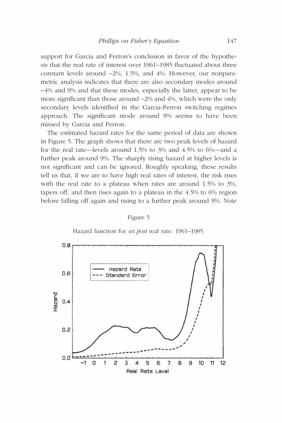
The estimated hazard rates for the same period of data are shownin Figure 5. The graph shows that there are two peak levels of hazardfor the real rate—levels around 1.5% to 3% and 4.5% to 6%—and afurther peak around 9%. The sharply rising hazard at higher levels isnot significant and can be ignored. Roughly speaking, these resultstell us that, if we are to have high real rates of interest, the risk riseswith the real rate to a plateau when rates are around 1.5% to 3%,tapers off, and then rises again to a plateau in the 4.5% to 6% regionbefore falling off again and rising to a further peak around 9%. Note


Figure 5

Hazard function for ex post real rate: 1961–1985.

that the very high peak at 9% is not significant, as the standard erroris rising quickly at this point. Moreover, the peak at 9% indicates thatif the real rate is to be as high as this, then it is very likely that it willbe in the region of 9%, given the observed data over the period1961–1985.

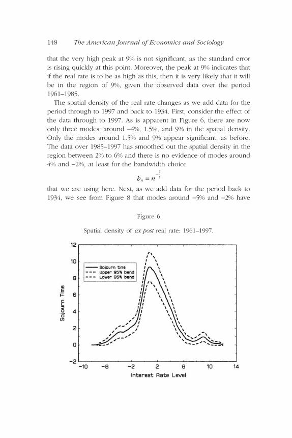
The spatial density of the real rate changes as we add data for theperiod through to 1997 and back to 1934. First, consider the effect ofthe data through to 1997. As is apparent in Figure 6, there are nowonly three modes: around -4%, 1.5%, and 9% in the spatial density.Only the modes around 1.5% and 9% appear significant, as before.The data over 1985–1997 has smoothed out the spatial density in theregion between 2% to 6% and there is no evidence of modes around4% and -2%, at least for the bandwidth choice

that we are using here. Next, as we add data for the period back to1934, we see from Figure 8 that modes around -5% and -2% have

h nn =-

1

5


Figure 6

Spatial density of ex post real rate: 1961–1997.

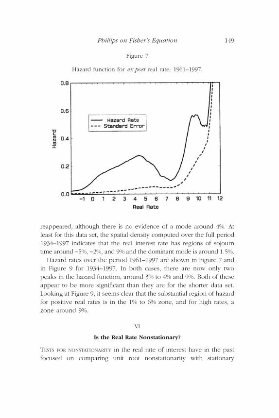
reappeared, although there is no evidence of a mode around 4%. Atleast for this data set, the spatial density computed over the full period1934–1997 indicates that the real interest rate has regions of sojourntime around -5%, -2%, and 9% and the dominant mode is around 1.5%.

Hazard rates over the period 1961–1997 are shown in Figure 7 andin Figure 9 for 1934–1997. In both cases, there are now only twopeaks in the hazard function, around 3% to 4% and 9%. Both of theseappear to be more significant than they are for the shorter data set.Looking at Figure 9, it seems clear that the substantial region of hazardfor positive real rates is in the 1% to 6% zone, and for high rates, azone around 9%.

VI

Is the Real Rate Nonstationary?

TESTS FOR NONSTATIONARITY in the real rate of interest have in the pastfocused on comparing unit root nonstationarity with stationary


Figure 7

Hazard function for ex post real rate: 1961–1997.

alternatives. We now consider a broader range of alternatives accom-modated by allowing for fractional integration.

Our approach is semi-parametric, so that we can retain as muchgenerality as possible regarding the generating mechanism for the realrate of interest rt. In particular, we consider a model for the ex postreal rate of the form

(19)

where ut is a zero mean stationary process with spectral density fuu(l)and is assumed to satisfy Assumption VIII.A in the Appendix. Byvirtue of Equation (19), the spectrum of rt has the following asymp-totic form in the vicinity of the origin

(20)

Several semi-parametric estimation procedures for d are available,and a brief review of some of the procedures is given in Robinson

ff

rruu

dll

l( )( )

~ , ~ .0

02

1 -( ) =L r udt t ,


Figure 8

Spatial density of real rate: 1934–1997.

(1995). We propose to use the modified log periodogram estimatorsuggested recently in Phillips (1999a). This estimator is, like log peri-odogram regression, simple to use, as it employs only least squarestechniques. Kim and Phillips (1999a) have shown that the estimatorhas good asymptotic properties that make it suitable for inference inpossibly nonstationary regions of d and have validated the construc-tion of confidence intervals that extend into the nonstationary region.It therefore seems well suited to the study of interest-rate data.

Log periodogram (LP) regression involves the least squares regres-sion (over s = 1, . . . , m for some m < n with

as n Æ •)

where Ir(ls) = |wr(ls)|2 is the periodogram and wr(ls) is the discrete

Fourier transform of rt, both evaluated at the fundamental frequencies

ln * * lnI c d er si sl l( )( ) = - - +1

2error,

10

m

m

n+ Æ


Figure 9

Hazard function for real rate: 1934–1997.

Modified LP regression involves the similar linear regression

(21)

in which the periodogram ordinates, Ir(ls), are replaced by the mod-ified periodogram ordinates Iv(ls) = |vx(ls)|

2, where

(22)

This procedure was suggested in Phillips (1999a), and Kim andPhillips (1999a) show that the modified LP estimator is consistentfor all d Œ (0, 2) and has the following limit theory

(23)

for

Thus, the limit theory for is the same as that of the conventionalLP estimator d* in the stationary case (Robinson 1995 and Hurvich;Deo, and Brodsky 1998). By contrast, the usual log periodogram esti-mator d* has a mixed normal limit theory when d = 1, as shown inPhillips (1999b) and is inconsistent when d > 1 (Kim and Phillips1999b). Thus, the modified regression in Equation (21) is especiallyuseful in the nonstationary case when

and the limit theory makes possible statistical testing and the con-struction of confidence intervals for d that extend into the nonsta-tionary case.

With this methodology and using

frequency ordinates, we found semi-parametric estimates of d in Equa-tion (19) for the ex post real rate for the three time periods 1961–1985,1961–1997, and 1934–1997. The results are given in Table 1.

For each period the estimates of d are greater than 0.5 and indi-

m n=3

4

d >1

2

d

d ŒÊË

ˆ¯

1

22, .

m d d Ndˆ ,-( ) æ Ææ ÊË

ˆ¯0

24

2p

d

v we

e

r

nx s r s

i

i

ns

sl l

p

l

l( ) = ( ) +-1 2

.

ln ˆ ˆ lnI c d ev si sl l( )( ) = - - +1

2error,

lp

s

s

ns m= =

21for , . . . , .


cate that the ex post real rate of interest is nonstationary. Moreover,the estimates of d are all quite close, which is interesting and perhapssurprising given that the sample path of rt varies substantially overthe full time period and that other approaches require multiple regimeshifts to model this data even over shorter periods. The confidenceintervals show that unit root nonstationarity and short memory areboth clearly rejected. However, in every case the confidence intervalsfor d include some long memory stationary alternatives with d lessthan 0.5 but greater than 0.4.

Thus, our estimates of d provide empirical evidence that supportsthe conclusion of Rose (1988) and Walsh (1987) that the real rate isnonstationary. But we reject unit root nonstationarity and the esti-mates of d are in every case not significantly greater than 0.5, so thereis also some support from our estimates for the hypothesis that thereal rate is marginally stationary but with very long memory.

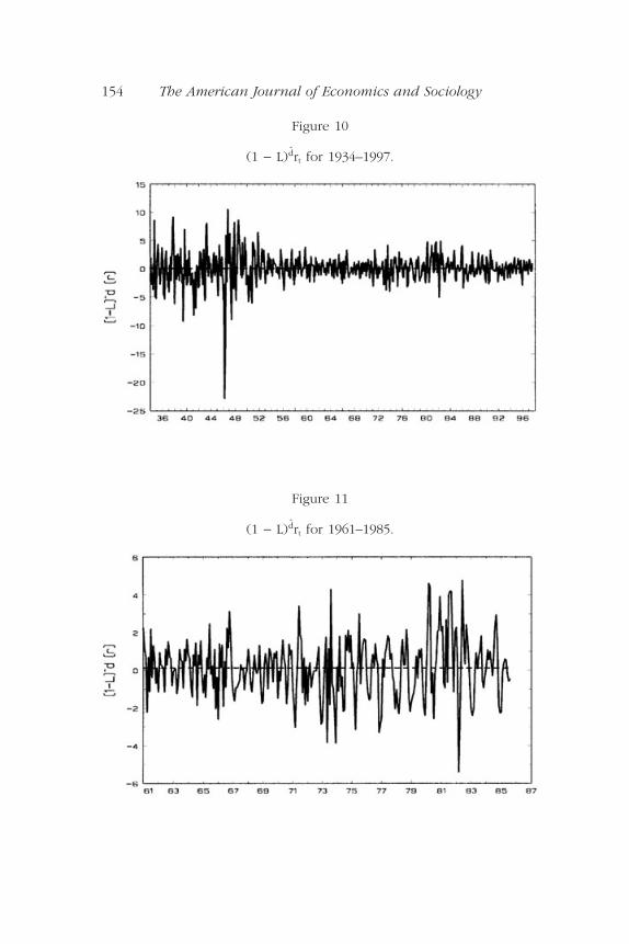
Figures 10–12 show the effect of d-differencing the real rate of interest using the relevant estimates for each of the subperiods. The figures also display the mean value of the residual series ût = (1 - L) rt for each period. As is apparent from the figures, ineach case ût appears to be stationary with short memory.

Finally, Figure 13 gives spatial density estimates for the differencedseries ût = (1 - L) rt calculated for each subperiod. The densities arecalculated here by normalizing the spatial densities in the same wayfor each subperiod—that is, by

in place of w 2

nh

1

nh

d

d

d


Table 1

Empirical Estimates of d: Ex Post Real Rate

Period s 95% Confidence Interval

1961–1985 0.6353 0.0761 [0.486,0.784]1961–1997 0.5538 0.0654 [0.426,0.682]1934–1997 0.5159 0.0532 [0.412,0.620]

dd


Figure 10

(1 - L) rt for 1934–1997.d

Figure 11

(1 - L) rt for 1961–1985.d


Figure 12

(1 - L) rt for 1961–1997.d

Figure 13

Densities of (1 - L) rt.d

in Equation (14)—so that they are directly comparable and corre-spond to conventional kernel estimates for a stationary density. As isapparent from the figure, the fitted densities are symmetric and quiteclose, although there is apparently greater dispersion in the case ofthe longer data set 1934–1997.

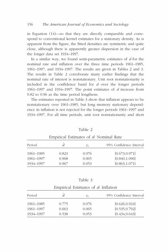
In a similar way, we found semi-parametric estimates of d for thenominal rate and inflation over the three time periods 1961–1985,1961–1997, and 1934–1997. The results are given in Tables 2 and 3.The results in Table 2 corroborate many earlier findings that thenominal rate of interest is nonstationary. Unit root nonstationarity isincluded in the confidence band for d over the longer periods1961–1997 and 1934–1997. The point estimates of d increase from0.82 to 0.96 as the time period lengthens.

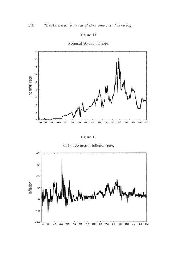
The estimates reported in Table 3 show that inflation appears to benonstationary over 1961–1985, but long memory stationary depend-ence in inflation is not rejected for the longer periods 1961–1997 and1934–1997. For all time periods, unit root nonstationarity and short


Table 2

Empirical Estimates of d: Nominal Rate


1961–1985 0.823 0.076 [0.673,0.971]1961–1997 0.968 0.065 [0.840,1.096]1934–1997 0.967 0.053 [0.863,1.071]

dd

Table 3

Empirical Estimates of d: Inflation


1961–1985 0.775 0.076 [0.626,0.924]1961–1997 0.663 0.065 [0.535,0.792]1934–1997 0.538 0.053 [0.434,0.643]

dd

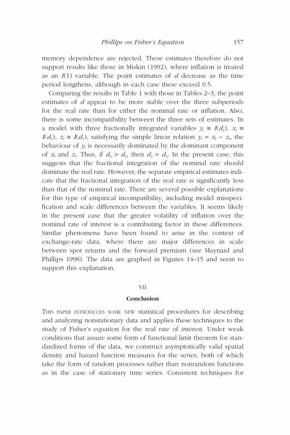
memory dependence are rejected. These estimates therefore do notsupport results like those in Miskin (1992), where inflation is treatedas an I(1) variable. The point estimates of d decrease as the timeperiod lengthens, although in each case these exceed 0.5.

Comparing the results in Table 1 with those in Tables 2–3, the pointestimates of d appear to be more stable over the three subperiodsfor the real rate than for either the nominal rate or inflation. Also,there is some incompatibility between the three sets of estimates. Ina model with three fractionally integrated variables yt ∫ I(dy), xt ∫I(dz), zt ∫ I(dz), satisfying the simple linear relation yt = xt - zt, thebehaviour of yt is necessarily dominated by the dominant componentof xt and zt. Thus, if dx > dz, then dy = dx. In the present case, thissuggests that the fractional integration of the nominal rate shoulddominate the real rate. However, the separate empirical estimates indi-cate that the fractional integration of the real rate is significantly lessthan that of the nominal rate. There are several possible explanationsfor this type of empirical incompatibility, including model misspeci-fication and scale differences between the variables. It seems likelyin the present case that the greater volatility of inflation over thenominal rate of interest is a contributing factor in these differences.Similar phenomena have been found to arise in the context ofexchange-rate data, where there are major differences in scalebetween spot returns and the forward premium (see Maynard andPhillips 1998). The data are graphed in Figures 14–15 and seem tosupport this explanation.

VII

Conclusion

THIS PAPER INTRODUCES SOME NEW statistical procedures for describingand analyzing nonstationary data and applies these techniques to thestudy of Fisher’s equation for the real rate of interest. Under weakconditions that assure some form of functional limit theorem for stan-dardized forms of the data, we construct asymptotically valid spatialdensity and hazard function measures for the series, both of whichtake the form of random processes rather than nonrandom functionsas in the case of stationary time series. Consistent techniques for



Figure 15

CPI three-month inflation rate.

Figure 14

Nominal 90-day TB rate.

estimating these quantities are given, together with a limit theory thatenables the measures to be used in inference.

Using these spatial density techniques, we analyze the ex post realrate of interest in the United States over the period 1934–1997. Resultsover the subperiod 1961–1985 provide some corroborating evidenceto support the conclusion of a recent study by Garcia and Perron(1994) that the real rate fluctuates about constant levels that changeover regimes. However, over the longer period 1934–1997, the regimechange approach requires many change points, seems artificial, andlacks parsimony.

An alternative semiparametric model is considered that allows forfractional integration in the real rate, including unit root nonstation-ary and stationary long-range dependence as special cases, to accountfor various types of long-run behavior and that retains generality withrespect to the modeling of the short-run component of the series.Through the fractional integration parameter in this model the extentof nonstationarity in the real rate can be directly measured. A newmodified log periodogram estimation of the fractional integrationparameter is performed using recently obtained asymptotic results byKim and Phillips (1999a) that apply in the nonstationary case. Empir-ical estimates of the fractional differencing parameter are computedfor the ex post rate over 1934–1997 and two shorter subperiods. Theresults confirm evidence of nonstationarity in the real rate for all timeperiods, and therefore generally support the conclusion reached byRose (1988). Our estimates also confirm Mishkin’s (1992) rejection ofunit root nonstationarity in the real rate of interest. However, althoughunit root nonstationarity and short memory can be rejected and pointestimates indicate nonstationarity, confidence intervals for the frac-tional differencing parameter are in the region [0.4, 0.6] and thereforedo not completely rule out the possibility of a stationary real rate ofinterest with very long-range dependence.

The fractional integration model for the real rate of interest seemsto be successful in transforming the data to stationarity over all threeperiods 1934–1997, 1961–1985, and 1961–1997, all with a very similarfractional integration parameter. In this respect, the model is at oncemore parsimonious and more generally applicable than a model withmany regime shifts.


VIII

Technical Appendix and Proofs

OUR APPROACH TO AN ASYMPTOTIC THEORY for spatial density and hazardrate estimation relies on recent work in Phillips and Park (1998), hereafter P2, for kernel density estimation and regression for nonsta-tionary time series. We only sketch the derivations we need here.

Suppose Xt is a unit root time series with differences DXt = ut andinitialization X0 that satisfy Conditions VIII.A and VIII.B below. Distantinitial conditions are permitted in VIII.B and play a role in the spatialdensity asymptotics. Conditions VIII.C and VIII.D relate to the kernelfunction and restrictions on the bandwidth h, and they are used inP2. Note the important difference between VIII.D and conventionalassumptions about bandwidth in kernel density estimation; here, thebandwidth can be of the form

so that bandwidths that increase with n are permissible. The band-width cannot decrease too fast or increase too fast, as n Æ •. Con-dition VIII.A allows for differences ut that follow a linear process andare standard (Phillips and Solo 1992). The higher moment conditionin VIII.A is useful in assuring the validity of a strong approximationto partial sums of ut.

A. Assumption

(a) ut is a linear process ut = C(L)et = cjet-j with C(1) π 0 and

(b) et is iid (0, s 2) with E(|ej|q) < • for some q > 2p > 4.

B. Assumption

The initial conditions of Xt are set at t = 0, and X0 has the followinggeneral form allowing for effects in the distant past

X u u jj

n

00

0= + ≥-=

[ ]

Âk

k, ,for some

j c jj

1

20

< •=

•Â .

S j =•

0

h cn knk= Œ - + -È

ÎÍ˘˚

, , ,1

4

1

12d d


where u is an Oa.s. (1) random variable with E(|u|p) for some p > 2.

C. Assumption

The kernel K(·) is a symmetric and nonnegative density with integrablecharacteristic function jK and satisfies the following conditions forsome r > 2:

D. Assumption

n1-d Æ •, and hn/n(1-d )/12 Æ 0 for some d > 0.

E. Proof of Theorem 3.1

The proof follows the same lines as that of Theorem 3.1 of P2. As inthat theorem, we need to augment the probability space so that astrong approximation to the limit Brownian motion B(r) of

can be used. The only changes in the proof are:

(i) Since ut is a linear process, we need to rely on extended versions of the preliminary Lemmas 5.5 and 5.7 in P2 that apply forlinear processes instead of iid random variables. These extensionsfollow in precisely the same way but make use of Lemma D of Phillips(1999b), which provides a strong approximation result for linearprocesses.

(ii) We use the consistent scale estimate 2 of the long-run vari-ance w2 = 2pfDx(0) in the definition of the spatial density estimate.This is not needed in Theorem 3.1 of P2 because chronological localtime B(r, a) = w-2LB(r, a) is used in P2 in place of local time.

(iii) Since 2 Æp w2, the resulting limit holds in probability ratherthan almost surely.

F. Proof of Theorem 3.2

From Lemma 2.9(d) of P2 we have

wL

w

n X nr-

[ ]

1

2

hn4

K s s K s ds K sr

s

( ) = ( ) < • ( ) < •-•

•

-•

•

Ú Ú1 2, , sup .


where Q(a, b) is a standard Brownian sheet. Then, using TheoremIII.A of P2, we have

where

which gives the stated mixed normal distribution

G. Proof of Theorem 4.1

By virtue of Theorem III.A and since s = s0 + a, we haven

MN L r a B K q q p K p dqdpB0 8 000

, , .- ( )( ) ( ) Ÿ( ) ( )( )••

ÚÚk

V K q q p K p dqdp K q q p K p dqdp= ( ) Ÿ( ) ( ) + -( ) Ÿ( ) -( )• •••

Ú ÚÚÚ 0 000,

c L r n s L r a B

cnh

Ks X

hL r a B

c c K cs X

nB g dg

n B B

nn t

nrt

nB

n n

r

n

ˆ , ,

ˆ,

-

=

[ ]

ÊË

ˆ¯ - - ( )( )È

ÎÍ˘˚

=-Ê

Ëˆ¯ - - ( )( )

È

ÎÍ

˘

˚˙

=-

- ( )ÏÌÓ¸˛

ÊË

ˆ¯

Â

Ú

1

20

2

10

2

0

0

k

wk

w -- - ( )( )ÈÎÍ

˘˚

+ ( )

=-

-ÏÌÓ¸˛

ÊË

ˆ¯ ( ) - - ( )( )È

ÎÍ˘˚

+ ( )

= ( ) --Ê

Ëˆ¯ -

-•

•

-•

•

Ú

Ú

L r a B o

c c K cs X

np L r p dp L r a B o

c K q L rs X

n

q

c

B p

n n n B B p

n Bn

,

, ,

,

0

00

0

1

1

k

k

LL r a B dq o

K q c L rs X

n

q

cL r a B dq o

K q Q L r a B q dq

L r

B p

n Bn

B p

d B

d B

,

, ,

, ,

,

- ( )( )ÈÎÍ

˘˚

+ ( )

= ( ) --Ê

Ëˆ¯ - - ( )( )È

ÎÍ˘˚

+ ( )

Æ ( ) - ( )( )( )

=

-•

•

-•

•

Ú

Ú

0

00

0

1

1

2

2

k

k

k

aa B K q Q q dq

L r a B N Vd B

- ( )( ) ( ) ( )

= - ( )( ) ( )

-•

•

Ú0

1

2

0

1

2

1

2 0

k

k

,

, , ,

2 1 1 2- +ÊË

ˆ¯ - ( )ÏÌÓ

¸˛

æ Ææ ( )( )ll

L t rs

L t r Q L t r sB Bd

B, , , , ,


giving the stated result.

H. Proof of Theorem 4.2

We have

(24)

Observe that

(25)

ˆ ,ˆ

ˆ

ˆ

L tp

n

dp

n nhK

p X

h

dp

n

nhK c

p X

n

dp

n

nhK c b

X

n

Bs

n ns

nt

nrt

n

ns

nt

nr

nt

n at

nr

nt

• •

=

[ ]

•

=

[ ]

•

=

[ ]

Ú ÚÂ

ÚÂ

ÚÂ

ÊË

ˆ¯ =

-ÊË

ˆ¯

=-È

ÎÍ˘˚

ÊË

ˆ¯

= -ÏÌÓ¸˛

w

w

w

2

1

2

1

2

1

ÊÊË

ˆ¯

= -ÏÌÓ¸˛

ÊË

ˆ¯

= -ÏÌÓ¸˛

ÊË

ˆ¯

=

[ ]

=

[ ]

Â

Â

db

nh cc a

X

n

nhc a

X

n

n nt

nr

nt

n t

nr

nt

ˆ

ˆ.

w

w

2

1

2

1

1K

K

c H r n s H r a B

cL t

s

n

L tp

n

dp

n

L t a B

L t c dc

n B B

n

B

Bs

n

B

Ba B

ˆ , ,

ˆ ,

ˆ ,

,

,.

-

•

- ( )

•

ÊË

ˆ¯ - - ( )( )È

ÎÍ˘˚

=

ÊË

ˆ¯

ÊË

ˆ¯

-- ( )( )

( )

È

Î

ÍÍÍÍ

˘

˚

˙˙˙˙Ú Ú

1

20

0

0

k

k

k

ˆ ,

ˆ ,

ˆ ,

,

,

,

,,

H ts

n

L ts

n

L tp

n

dp

n

L t a B

L t b B db

L t a B

L t c dcH t a B

B

B

Bs

n

pB

Ba

B

Ba B

B

ÊË

ˆ¯ =

ÊË

ˆ¯

ÊË

ˆ¯

Æ- ( )( )- ( )( )

=- ( )( )

( )= - ( )( )

•

•

- ( )

•

Ú

Ú

Ú

0

0

00

0

k

k

kk

k


Now, under the assumption that ( 2 - w2) = op(1), using the strong

approximation

as in P2 and proceeding as in the proof of Theorem 3.1 of P2, we get

(26)

since

from the given tail behavior of the kernel K(s) and where r > 2 (seeAssumption VIII.C).

It follows from Equation (24)–(25) and Theorem 3.2 that

K c a B c K s ds

Oc

c a B

Oc

c a B

nc a B c

nr

nr

n- ( ) -{ }( ) = ( )

=

ÊËÁ

ˆ¯ < - ( )

+ ÊËÁ

ˆ¯ > - ( )

Ï

ÌÔÔ

ÓÔÔ

- ( )-{ }

•

-

-

Ú0

2 1 0

2 1 0

0

1

11

k

k

k

k

for

for

ˆ

,

,

ww k

w k

w

2

1

2

00

20

2

1

1

nc a

X

nc a B B s ds o

c

c a B c L r c dc

oc

L r c dc

t

nr

nt r

n pn

n B

pn

Ba

K K

K

=

[ ]

-•

•

Â Ú

Ú

-ÏÌÓ¸˛

ÊË

ˆ¯ = - ( ) - ( ){ }( ) + Ê

Ëˆ¯

= - ( ) -{ }( ) ( ) +

ÊË

ˆ¯

= ( )-- ( )

•

Ú + ÊË

ˆ¯B

pn

oc0

1k

X

nB B r o nnr

a sP[ ] - +

= ( ) + ( ) + ÊË

ˆ¯0

1

2

1

k . .

wcn


giving the required result.

I. Notation

Æa.s. almost sure convergence [·] integer part of=d distributional equivalence r ^ s min(r, s):= definitional equality ∫ equivalence in oa.s.(1) tends to zero almost surely distributionÆp convergence in probability op(1) tends to zero in (a)k (a)(a + 1) . . . (a + k - 1) probabilityfi, Æd weak convergence

J. Data Sources

(a) Consumer Price IndexNot seasonally adjustedArea: U.S. city average (i.e., urban)Items: All itemsBase: 1982–1984 = 100Source: Bureau of Labor Statistics, Monthly Labor ReviewCode: CUUR0000SA0

c H r n s H r a B

cL t

p

n

L t c dc oc

L t a B

L t c dc

n B B

n

B

Ba B

pn

B

Ba B

ˆ , ,

ˆ ,

,

,

,

-

- ( )

•

- ( )

•

ÊË

ˆ¯ - - ( )( )È

ÎÍ˘˚

=

ÊË

ˆ¯

( ) + ÊË

ˆ¯

-- ( )( )

( )

È

Î

ÍÍÍ

˘

˚

˙˙

Ú Ú

1

20

0

0 0

1

k

k

k k˙

=( )

ÊË

ˆ¯ - - ( )( )È

ÎÍ˘˚

fi( )

( ) - ( )( )( )

∫- ( )

- ( )

•

- ( )

• -•

•

Ú

ÚÚ

1

2

0 8

0

0

0

0

20

L t c dcc L t

s

nL t a B

L t c dcK q Q L r a B q dq

MN KL r a B

Ba B

n B B

Ba B

B

B

,

ˆ , ,

,, ,

,,

k

k

k

k

k(( )

( )( )Ê

Ë

ÁÁÁ

ˆ

¯

˜˜

- ( )

•

Ú L r s dsBa B

,,

0

2

k


(b) Three-Month Treasury Bill RateSecondary marketAverage of daily closing bidAnnualized using a 360-day year for bank interestQuoted on a discount basisSource: Board of Governors of the Federal Reserve System,

Federal Reserve BulletinCode: TB3MS

Notes

1. Fisher (1896) credited Marshall (1895) for making the distinctionbetween real and nominal interest. It appears the idea that expected infla-tion affects interest rates can be traced to earlier political speeches and polit-ical economy pamphlets. Howitt (1992) and Laidler (1991) provide somefurther information about the history of the concept and the distinctionbetween real and nominal rates. Fisher seems to have been the first toconduct a sustained study and to explore the matter in serious empiricalresearch.

2. The reader is referred to Revuz and Yor (1994) for much of the under-lying stochastic process theory used here. Good introductions are Chung andWilliams (1990) and Karatzas and Shreve (1991).

3. In these and in our other calculations we used a bandwidth of

References

Akonom, J., and C. Gourieroux. (1987). A Functional Limit Theorem for Fractional Processes. Unpublished ms.

Chung, K. L., and R. J. Williams. (1990). Introduction to Stochastic Integra-tion. 2nd ed. Boston: Birkhäuser.

Fama, E. F. (1975). “Short Term Interest Rates as Predictors of Inflation.” American Economic Review 65: 269–282.

Fisher, I. (1896). “Appreciation and Interest.” AEA Publications 3(11): 331–442.——. (1930). The Theory of Interest. New York: Macmillan.Garcia, R., and P. Perron. (1996). “An Analysis of the Real Rate of Interest

Under Regime Shifts.” Review of Economics and Statistics 111–125.Gil-Alana, L. A., and P. M. Robinson. (1997). “Testing for a Unit Root and

Other Nonstationary Hypotheses in Macroeconomic Time Series.”Journal of Econometrics 80: 241–268.

Howitt, P. (1992). “Fisher Effect.” In New Palgrave Dictionary of Money andFinance. London: Macmillan.

h nn =-

1

5 .


Hurvich, C. M., R. Deo, and J. Brodsky. (1998). “The Mean Squared Error ofGeweke and Porter-Hudak’s Estimator of the Memory Parameter of aLong-Memory Time Series.” Journal of Time Series Analysis 19: 19–46.

Karatzas, I., and S. E. Shreve. (1988). Brownian Motion and Stochastic Calculus. New York: Springer-Verlag.

Kim, C. S., and P. C. B. Phillips. (1999a). Modified Log Periodogram Regres-sion. Yale University, mimeo.

——. (1999b). Log Periodogram Regression: The Nonstationary Case. Yale Uni-versity, mimeo.

Laidler, D. (1991). The Golden Age of the Quantity Theory. Hemel Hempstead:Philip Allan.

Mandlebrot, B., and J. van Ness. (1968). “Fractional Brownian Motion, Frac-tional Noises and Applications.” SIAM Review 10: 422–437.

Marshall, A. (1895). Principles of Economics. 3rd ed. London: Macmillan.Maynard, A., and P. C. B. Phillips. (1998). Rethinking an Old Empirical

Puzzle: Econometric Evidence on the Forward Discount Anomaly. YaleUniversity, mimeo.

Mishkin, F. S. (1981). “The Real Rate of Interest: An Empirical Investigation.The Cost and Consequences of Inflation.” Carnegie-Rochester Confer-ence Series on Public Policy 15: 151–200.

——. (1992). “Is the Fisher Effect for Real?” Journal of Monetary Economics30: 195–215.

Phillips, P. C. B. (1987). “Towards a Unified Asymptotic Theory for Auto-regression.” Biometrika 74: 535–547.

——. (1999a). Discrete Fourier Transforms of Fractional Processes. Yale University, mimeo.

——. (1999b). Unit Root Log Periodogram Regression. Yale University, mimeo.Phillips, P. C. B., and J. Y. Park. (1998). Nonstationary Density Estimation

and Kernel Autoregression. Yale University, mimeo.Phillips, P. C. B., and V. Solo. (1992). “Asymptotics for Linear Processes.”

Annals of Statistics 20: 971–1001.Protter, P. (1990). Stochastic Integration and Differential Equations. New

York: Springer.Revuz, D., and M. Yor. (1994). Continuous Martingales and Brownian

Motion. 2nd ed. New York: Springer-Verlag.Robinson, P. M. (1994). “Time Series with Strong Dependence.” In Advances

in Econometrics, Sixth World Congress, 1C. Ed. A. Sims. Cambridge:Cambridge University Press.

——. (1995). “Gaussian Semiparametric Estimation of Long Range Depen-dence.” Annals of Statistics 23: 1630–1661.

Rose, A. K. (1988). “Is the Real Interest Rate Stable?” Journal of Finance 43:1095–1112.

Silverman, B. W. (1986). Density Estimation for Statistics and Data Analysis.London: Chapman and Hall.


Summers, L. H. (1983). “The Non-Adjustment of Nominal Interest Rates: AStudy of the Fisher Effect.” In Macroeconomics, Prices, and Quantities:Essays in Memory of Arthur M. Okun. Ed. James Tobin. Washington, DC:Brookings Institution.

Taqqu, M. S. (1975). “Weak Convergence to Fractional Brownian Motion andto the Rosenblatt Process.” Z. Wahrsch. Verw. Gebiete 31: 287–302.

Tyurin, K., and P. C. B. Phillips. (1999). The Occupation Density of FractionalBrownian Motion and Some of Its Applications. Yale University, mimeo.

Walsh, C. E. (1987) “Three Questions Concerning Nominal and Real InterestRates.” Economic Review 4: 5–20.


ECONOMETRIC ANALYSIS OF FISHER’S EQUATION BY PETER...

Documents

Transcript of ECONOMETRIC ANALYSIS OF FISHER’S EQUATION BY PETER...