Econ 230B – Graduate Public Economics

Models of the wealth distribution

Gabriel Zucman

zucman@berkeley.edu

1

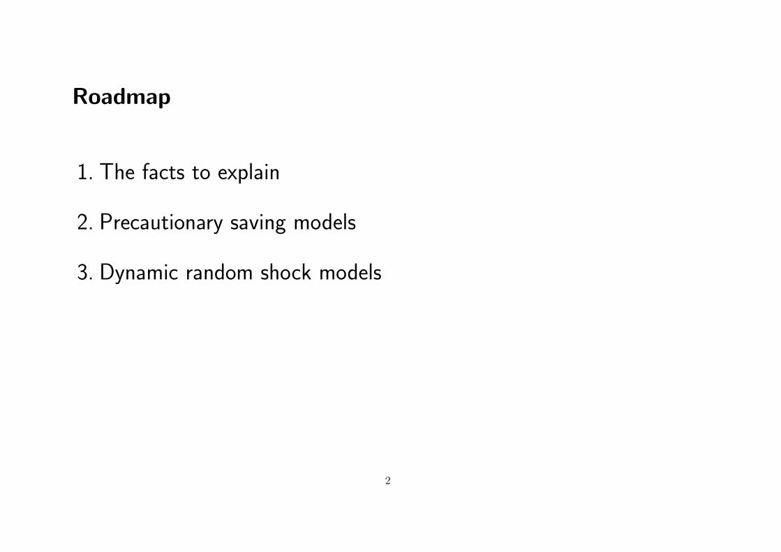
Roadmap

1. The facts to explain

2. Precautionary saving models

3. Dynamic random shock models

2

1 The facts to explain

• Fact 1: Wealth is very unequally distributed, much more thanlabor income

• Fact 2: Wealth concentration tends to be particularly high inlow-growth societies (e.g., 18th-19th century)

• Fact 3: Wealth inequality has been rising in recent decades butthere is a diversity of national trajectories

3

0%

5%

10%

15%

20%

25%

30%

35%

40%

45%

1962 1966 1970 1974 1978 1982 1986 1990 1994 1998 2002 2006 2010 2014

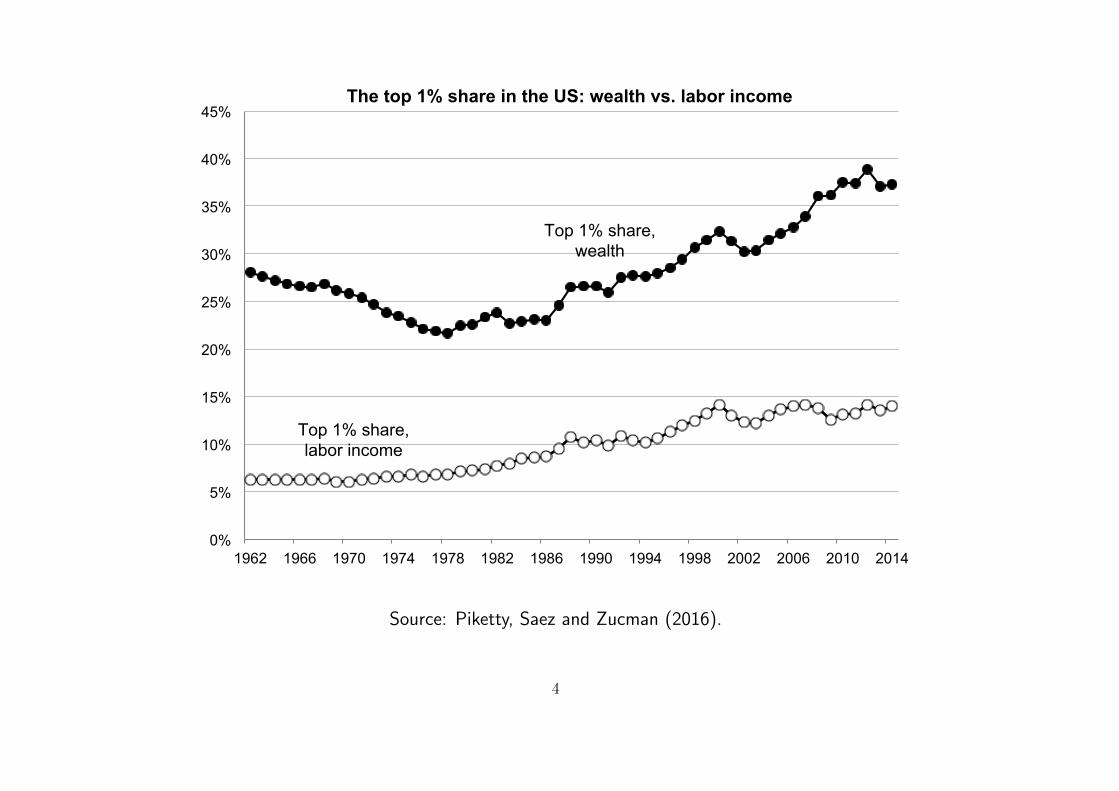
The top 1% share in the US: wealth vs. labor income

Top 1% share, wealth

Top 1% share, labor income

Source: Piketty, Saez and Zucman (2016).

4

3

particular attention to the role of housing in understanding the dynamics of wealth

concentration. The new estimates represent, we believe, an advance on those available

to date, but they should be viewed in the context of a variety of potential sources of

error, arising both from the underlying method and from the reliance on tax data. In

Section 5, we consider the internal validity of the estimates presented here by

addressing the main problems with the methods used in their construction, and in

Section 6 we apply checks on their external validity through an examination as to how

far they can be triangulated with evidence from other sources.

Source: Table G1.

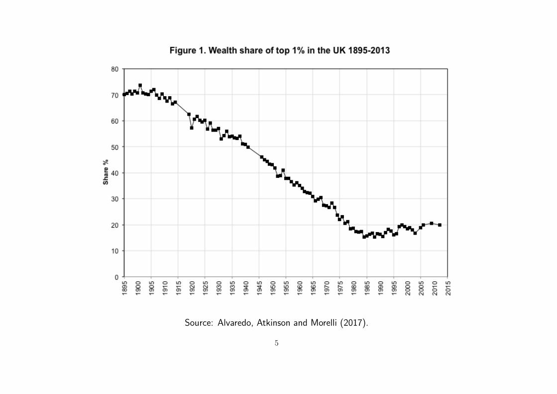
The new evidence about top wealth shares for the UK is compared in Section 7 with the

evidence for top wealth shares in the United States (US). There has long been interest in

contrasting wealth distributions in the UK and the US (for example, Lydall and Lansing,

1959, and Lampman, 1962). The juxtaposition of the two countries is of particular

relevance given the recent critical reviews of the long-run US evidence (Kopczuk, 2015

and 2016, and Sutch, 2015), and the publication of alternative estimates by Bricker et al,

2016, and Saez and Zucman, 2016, the latter finding a particularly sharp rise in the very

top wealth shares. Comparisons made half a century ago found wealth to be more

concentrated in England, but today the US is seen as the home of major concentrations.

If so, when did the countries change position? There are significant differences in the

nature of the estate data – in coverage and in the process of assembly – but the sources

are sufficiently similar to make the comparison a meaningful one.

Source: Alvaredo, Atkinson and Morelli (2017).

5

10%

20%

30%

40%

50%

60%

70%

80%

1890 1900 1910 1920 1930 1940 1950 1960 1970 1980 1990 2000 2010

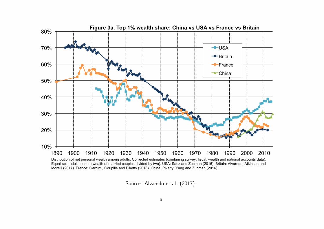
Figure 3a. Top 1% wealth share: China vs USA vs France vs Britain

USA

Britain

France

China

Distribution of net personal wealth among adults. Corrected estimates (combining survey, fiscal, wealth and national accounts data). Equal-split-adults series (wealth of married couples divided by two). USA: Saez and Zucman (2016). Britain: Alvaredo, Atkinson and Morelli (2017). France: Garbinti, Goupille and Piketty (2016). China: Piketty, Yang and Zucman (2016).

Source: Alvaredo et al. (2017).

6

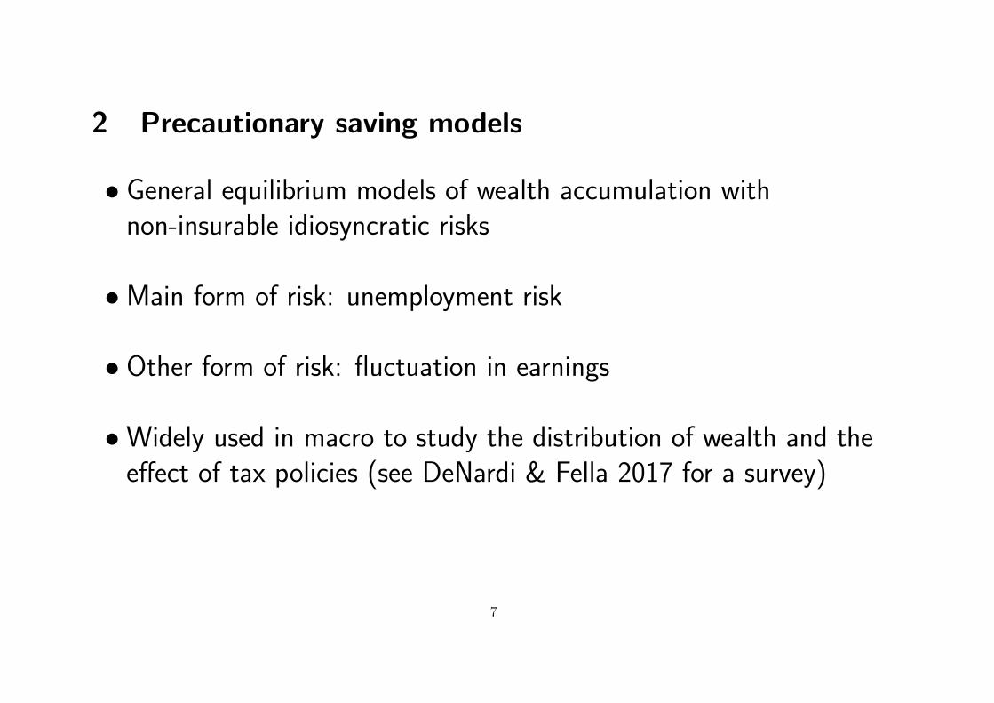
2 Precautionary saving models

• General equilibrium models of wealth accumulation withnon-insurable idiosyncratic risks

•Main form of risk: unemployment risk

• Other form of risk: fluctuation in earnings

•Widely used in macro to study the distribution of wealth and theeffect of tax policies (see DeNardi & Fella 2017 for a survey)

7

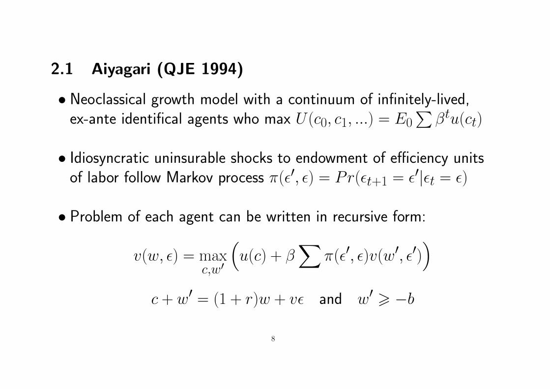
2.1 Aiyagari (QJE 1994)

• Neoclassical growth model with a continuum of infinitely-lived,ex-ante identifical agents who max U(c0, c1, ...) = E0

∑βtu(ct)

• Idiosyncratic uninsurable shocks to endowment of efficiency unitsof labor follow Markov process π(ε′, ε) = Pr(εt+1 = ε′|εt = ε)

• Problem of each agent can be written in recursive form:

v(w, ε) = maxc,w′

(u(c) + β

∑π(ε′, ε)v(w′, ε′)

)c + w′ = (1 + r)w + vε and w′ > −b

8

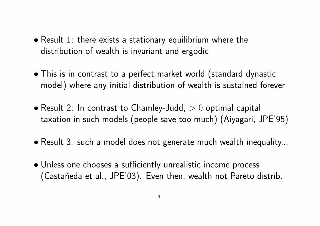
• Result 1: there exists a stationary equilibrium where thedistribution of wealth is invariant and ergodic

• This is in contrast to a perfect market world (standard dynasticmodel) where any initial distribution of wealth is sustained forever

• Result 2: In contrast to Chamley-Judd, > 0 optimal capitaltaxation in such models (people save too much) (Aiyagari, JPE’95)

• Result 3: such a model does not generate much wealth inequality...

• Unless one chooses a sufficiently unrealistic income process(Castaneda et al., JPE’03). Even then, wealth not Pareto distrib.

9

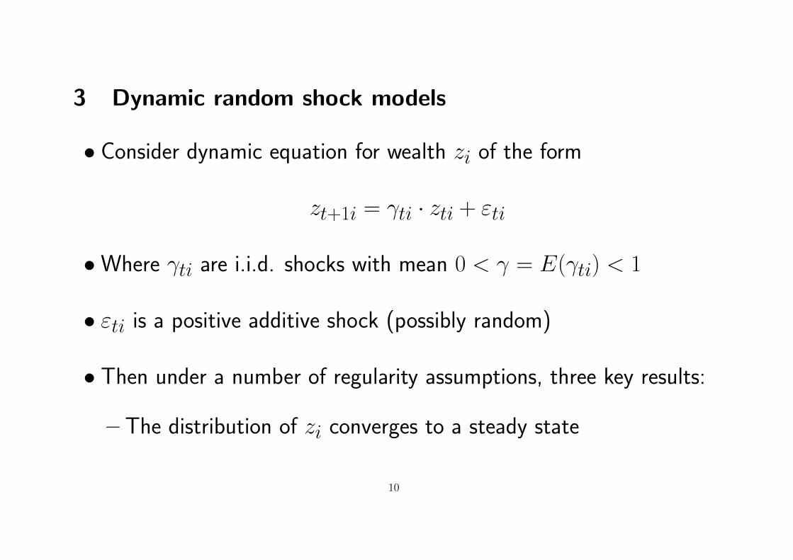
3 Dynamic random shock models

• Consider dynamic equation for wealth zi of the form

zt+1i = γti · zti + εti

•Where γti are i.i.d. shocks with mean 0 < γ = E(γti) < 1

• εti is a positive additive shock (possibly random)

• Then under a number of regularity assumptions, three key results:

– The distribution of zi converges to a steady state

10

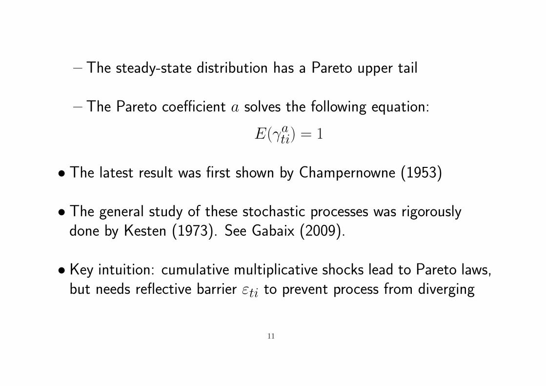
– The steady-state distribution has a Pareto upper tail

– The Pareto coefficient a solves the following equation:

E(γati) = 1

• The latest result was first shown by Champernowne (1953)

• The general study of these stochastic processes was rigorouslydone by Kesten (1973). See Gabaix (2009).

• Key intuition: cumulative multiplicative shocks lead to Pareto laws,but needs reflective barrier εti to prevent process from diverging

11

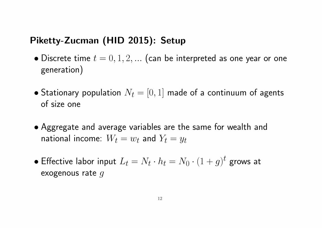
Piketty-Zucman (HID 2015): Setup

• Discrete time t = 0, 1, 2, ... (can be interpreted as one year or onegeneration)

• Stationary population Nt = [0, 1] made of a continuum of agentsof size one

• Aggregate and average variables are the same for wealth andnational income: Wt = wt and Yt = yt

• Effective labor input Lt = Nt · ht = N0 · (1 + g)t grows atexogenous rate g

12

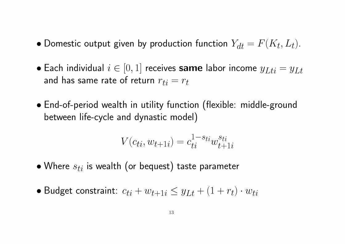
• Domestic output given by production function Ydt = F (Kt, Lt).

• Each individual i ∈ [0, 1] receives same labor income yLti = yLtand has same rate of return rti = rt

• End-of-period wealth in utility function (flexible: middle-groundbetween life-cycle and dynastic model)

V (cti, wt+1i) = c1−stiti w

stit+1i

•Where sti is wealth (or bequest) taste parameter

• Budget constraint: cti + wt+1i ≤ yLt + (1 + rt) · wti

13

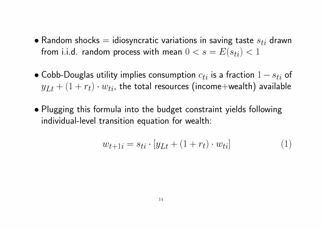
• Random shocks = idiosyncratic variations in saving taste sti drawnfrom i.i.d. random process with mean 0 < s = E(sti) < 1

• Cobb-Douglas utility implies consumption cti is a fraction 1− sti ofyLt + (1 + rt) · wti, the total resources (income+wealth) available

• Plugging this formula into the budget constraint yields followingindividual-level transition equation for wealth:

wt+1i = sti · [yLt + (1 + rt) · wti] (1)

14

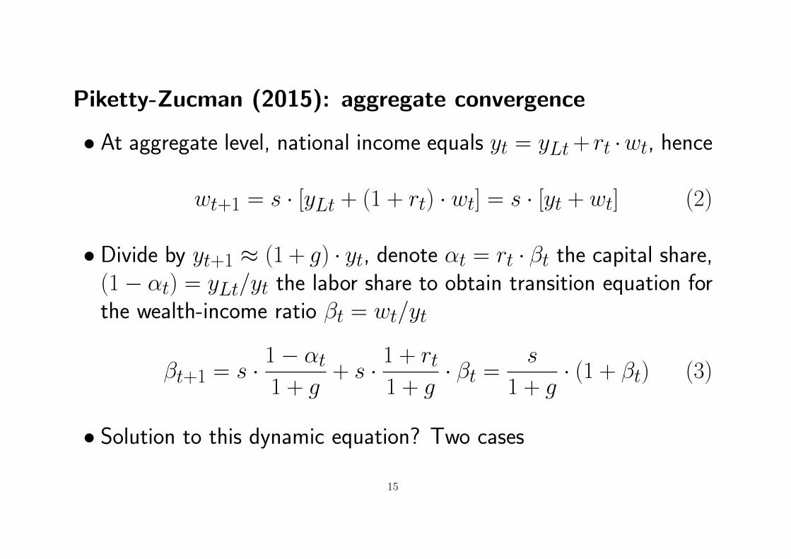
Piketty-Zucman (2015): aggregate convergence

• At aggregate level, national income equals yt = yLt+ rt ·wt, hence

wt+1 = s · [yLt + (1 + rt) · wt] = s · [yt + wt] (2)

• Divide by yt+1 ≈ (1 + g) · yt, denote αt = rt · βt the capital share,(1− αt) = yLt/yt the labor share to obtain transition equation forthe wealth-income ratio βt = wt/yt

βt+1 = s · 1− αt1 + g

+ s · 1 + rt1 + g

· βt =s

1 + g· (1 + βt) (3)

• Solution to this dynamic equation? Two cases

15

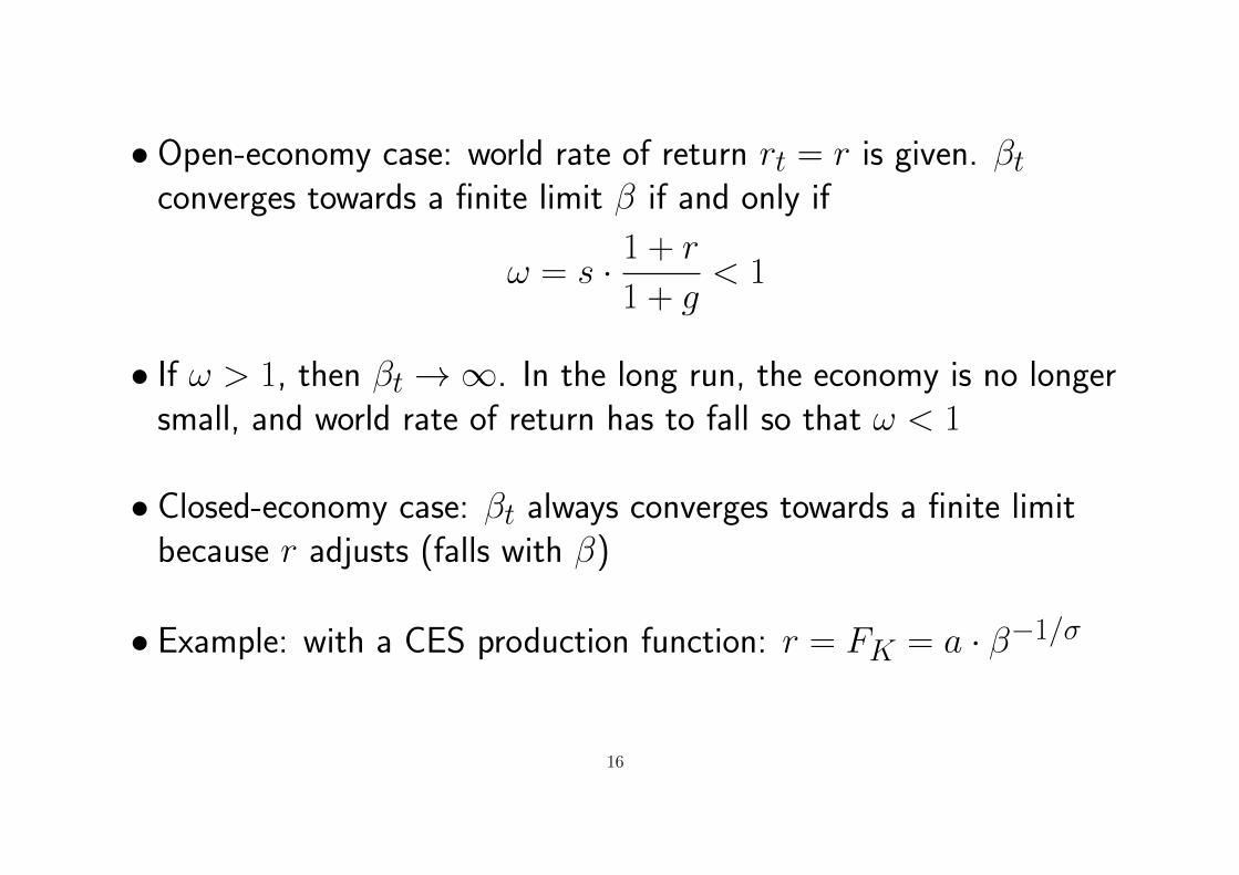
• Open-economy case: world rate of return rt = r is given. βtconverges towards a finite limit β if and only if

ω = s · 1 + r

1 + g< 1

• If ω > 1, then βt→∞. In the long run, the economy is no longersmall, and world rate of return has to fall so that ω < 1

• Closed-economy case: βt always converges towards a finite limitbecause r adjusts (falls with β)

• Example: with a CES production function: r = FK = a · β−1/σ

16

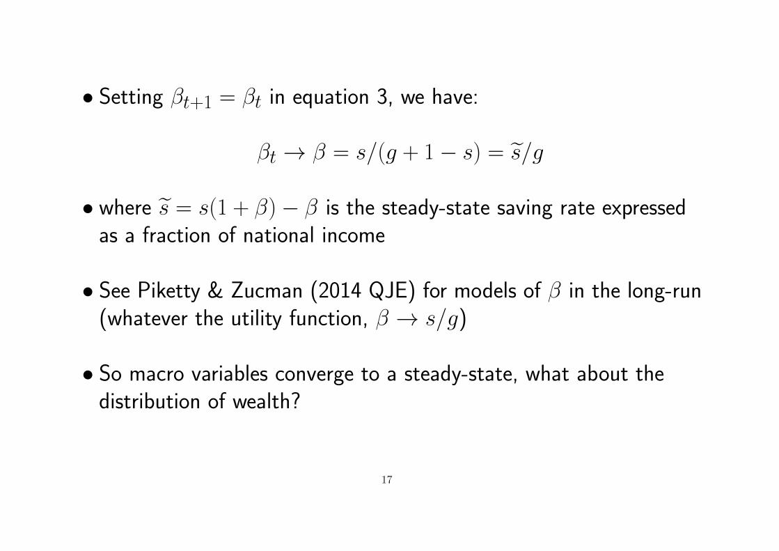
• Setting βt+1 = βt in equation 3, we have:

βt→ β = s/(g + 1− s) = s/g

• where s = s(1 + β)− β is the steady-state saving rate expressedas a fraction of national income

• See Piketty & Zucman (2014 QJE) for models of β in the long-run(whatever the utility function, β → s/g)

• So macro variables converge to a steady-state, what about thedistribution of wealth?

17

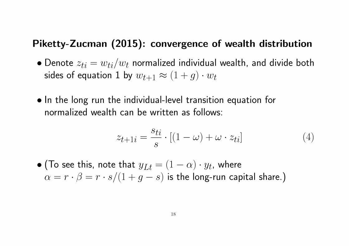
Piketty-Zucman (2015): convergence of wealth distribution

• Denote zti = wti/wt normalized individual wealth, and divide bothsides of equation 1 by wt+1 ≈ (1 + g) · wt

• In the long run the individual-level transition equation fornormalized wealth can be written as follows:

zt+1i =stis· [(1− ω) + ω · zti] (4)

• (To see this, note that yLt = (1− α) · yt, whereα = r · β = r · s/(1 + g − s) is the long-run capital share.)

18

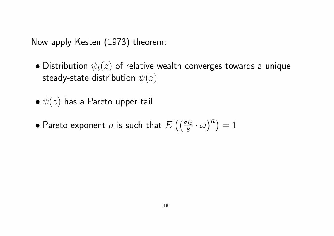
Now apply Kesten (1973) theorem:

• Distribution ψt(z) of relative wealth converges towards a uniquesteady-state distribution ψ(z)

• ψ(z) has a Pareto upper tail

• Pareto exponent a is such that E((sti

s · ω)a)

= 1

19

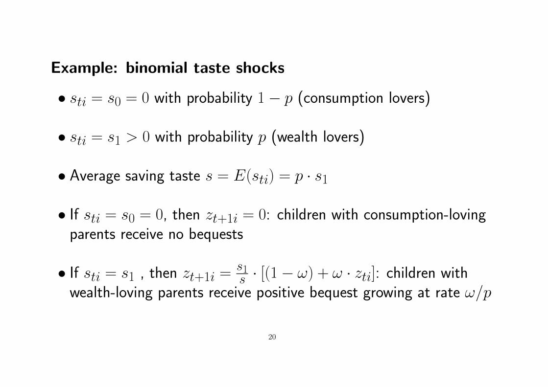
Example: binomial taste shocks

• sti = s0 = 0 with probability 1− p (consumption lovers)

• sti = s1 > 0 with probability p (wealth lovers)

• Average saving taste s = E(sti) = p · s1

• If sti = s0 = 0, then zt+1i = 0: children with consumption-lovingparents receive no bequests

• If sti = s1 , then zt+1i =s1s · [(1− ω) + ω · zti]: children with

wealth-loving parents receive positive bequest growing at rate ω/p

20

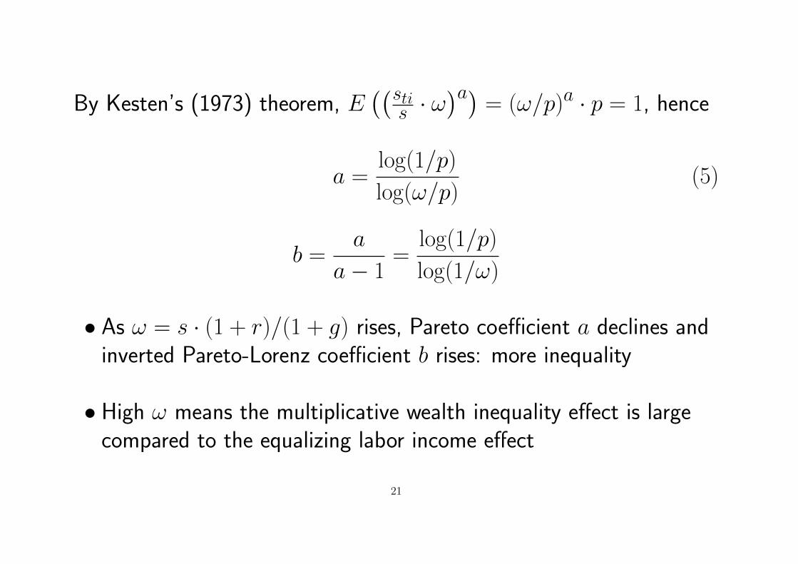
By Kesten’s (1973) theorem, E((sti

s · ω)a)

= (ω/p)a · p = 1, hence

a =log(1/p)

log(ω/p)(5)

b =a

a− 1=

log(1/p)

log(1/ω)

• As ω = s · (1 + r)/(1 + g) rises, Pareto coefficient a declines andinverted Pareto-Lorenz coefficient b rises: more inequality

• High ω means the multiplicative wealth inequality effect is largecompared to the equalizing labor income effect

21

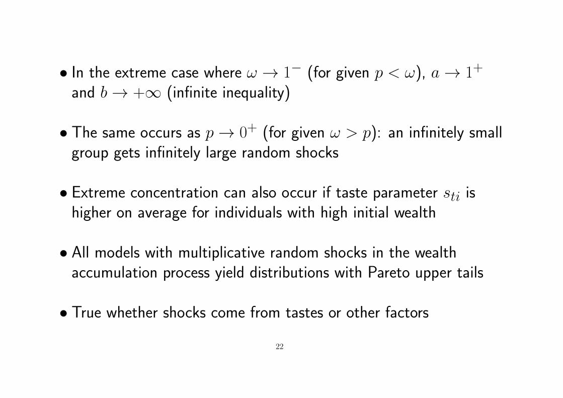
• In the extreme case where ω → 1− (for given p < ω), a→ 1+

and b→ +∞ (infinite inequality)

• The same occurs as p→ 0+ (for given ω > p): an infinitely smallgroup gets infinitely large random shocks

• Extreme concentration can also occur if taste parameter sti ishigher on average for individuals with high initial wealth

• All models with multiplicative random shocks in the wealthaccumulation process yield distributions with Pareto upper tails

• True whether shocks come from tastes or other factors

22

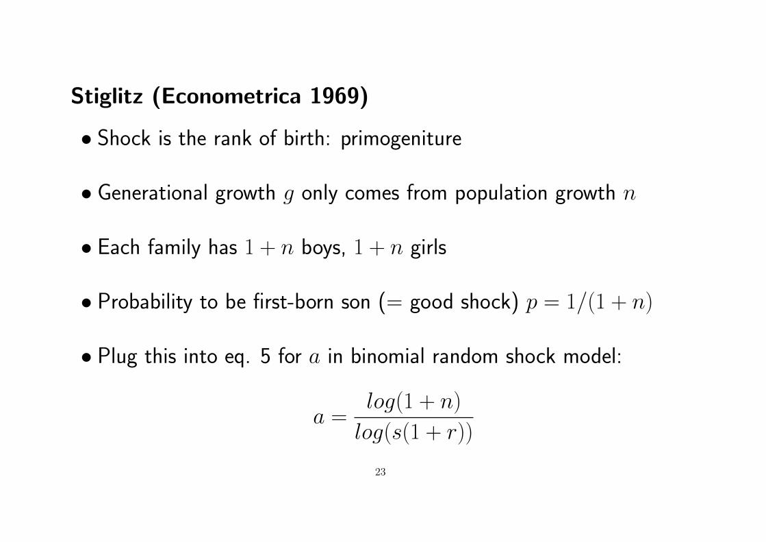
Stiglitz (Econometrica 1969)

• Shock is the rank of birth: primogeniture

• Generational growth g only comes from population growth n

• Each family has 1 + n boys, 1 + n girls

• Probability to be first-born son (= good shock) p = 1/(1 + n)

• Plug this into eq. 5 for a in binomial random shock model:

a =log(1 + n)

log(s(1 + r))

23

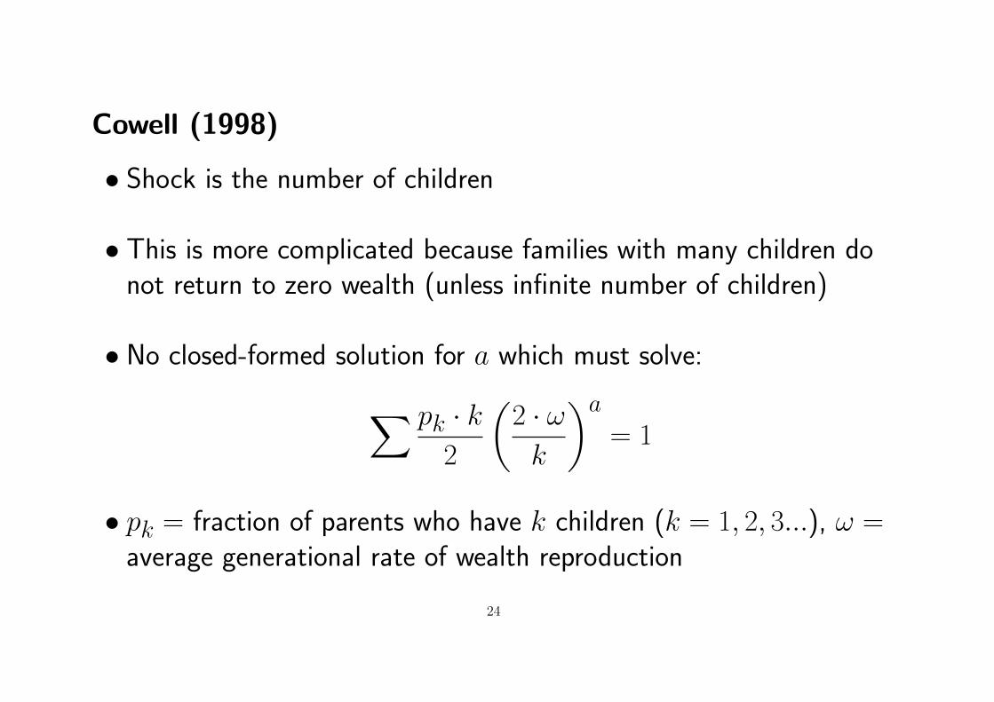
Cowell (1998)

• Shock is the number of children

• This is more complicated because families with many children donot return to zero wealth (unless infinite number of children)

• No closed-formed solution for a which must solve:∑ pk · k2

(2 · ωk

)a= 1

• pk = fraction of parents who have k children (k = 1, 2, 3...), ω =average generational rate of wealth reproduction

24

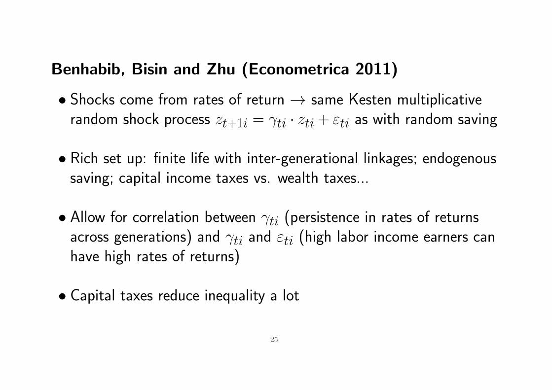
Benhabib, Bisin and Zhu (Econometrica 2011)

• Shocks come from rates of return → same Kesten multiplicativerandom shock process zt+1i = γti · zti+ εti as with random saving

• Rich set up: finite life with inter-generational linkages; endogenoussaving; capital income taxes vs. wealth taxes...

• Allow for correlation between γti (persistence in rates of returnsacross generations) and γti and εti (high labor income earners canhave high rates of returns)

• Capital taxes reduce inequality a lot

25

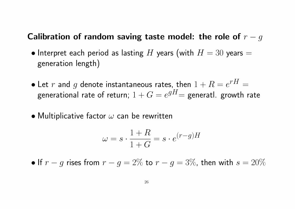
Calibration of random saving taste model: the role of r − g

• Interpret each period as lasting H years (with H = 30 years =generation length)

• Let r and g denote instantaneous rates, then 1 +R = erH =generational rate of return; 1 +G = egH= generatl. growth rate

•Multiplicative factor ω can be rewritten

ω = s · 1 +R

1 +G= s · e(r−g)H

• If r − g rises from r − g = 2% to r − g = 3%, then with s = 20%

26

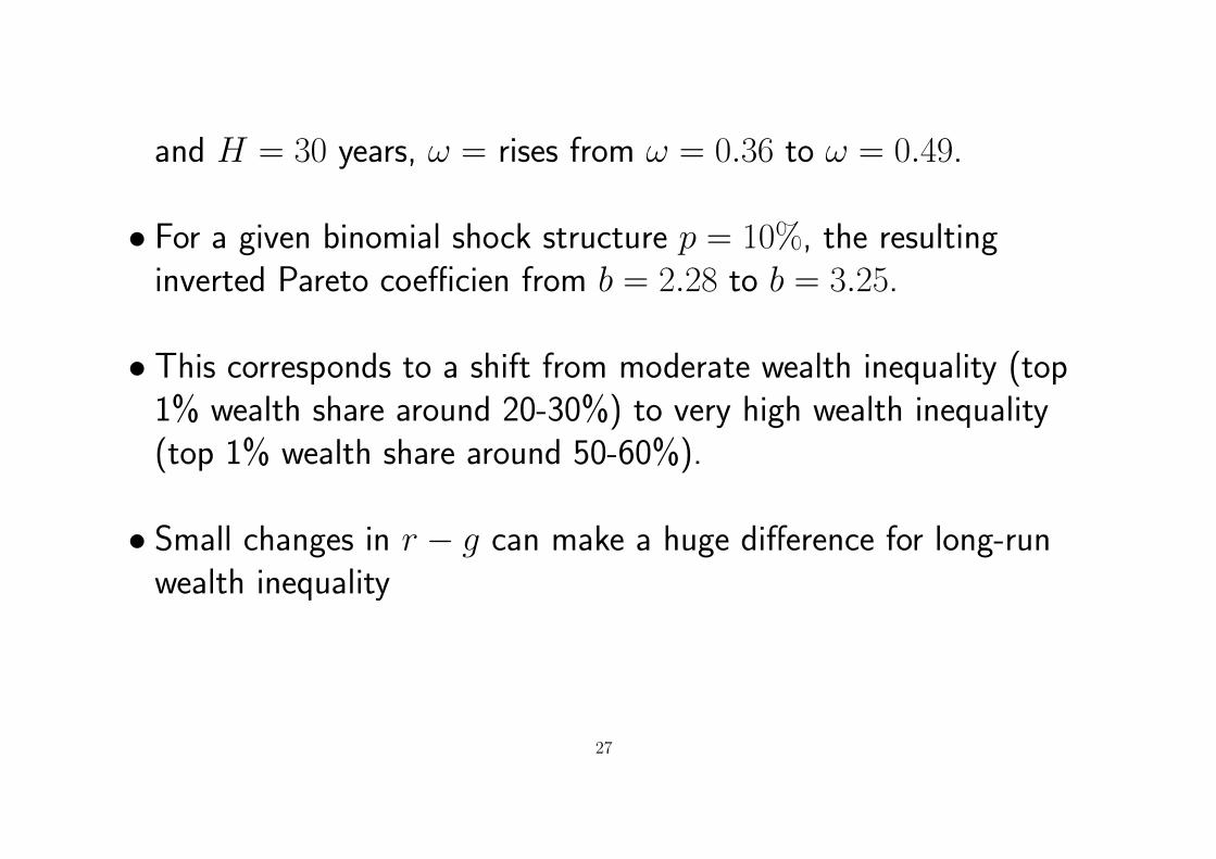
and H = 30 years, ω = rises from ω = 0.36 to ω = 0.49.

• For a given binomial shock structure p = 10%, the resultinginverted Pareto coefficien from b = 2.28 to b = 3.25.

• This corresponds to a shift from moderate wealth inequality (top1% wealth share around 20-30%) to very high wealth inequality(top 1% wealth share around 50-60%).

• Small changes in r − g can make a huge difference for long-runwealth inequality

27

Intuition: why r − g matters

• r − g magnifies any initial wealth inequality

• Ex: if g = 1 and r = 4%, then a person whose income only derivesfrom wealth W (hence has income rW ) needs to save onlyg/r=25% for her wealth to grow as fast as the economy

•With taxes in the model, r must be replaced by the after-tax rateof return r = (1− τ ) · r

•Where τ is the equivalent comprehensive tax rate on capitalincome, including all taxes on both flows and stocks.

28

Level and changes in r − g gap can contribute to explain:

• Extreme wealth concentration in Europe in 19c and during most ofhuman history (high r − g)

• Lower wealth inequality in the US in 19c (high g)

• Long-lasting decline of wealth concentration in 20c (low r due toshocks, high g)

• Return of high wealth concentration since late 20c/early 21c(lowering of g, and rise of r, in particular due to tax competition)

29

0%

1%

2%

3%

4%

5%

6%

0-1000 1000-1500 1500-1700 1700-1820 1820-1913 1913-1950 1950-2012 2012-2050 2050-2100

Ann

ual r

ate

of re

turn

or r

ate

of g

row

th

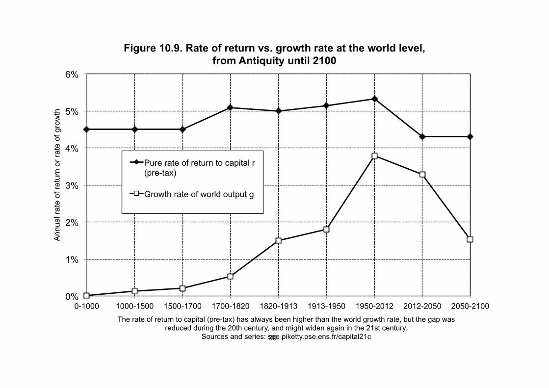
The rate of return to capital (pre-tax) has always been higher than the world growth rate, but the gap was reduced during the 20th century, and might widen again in the 21st century.

Sources and series: see piketty.pse.ens.fr/capital21c

Figure 10.9. Rate of return vs. growth rate at the world level, from Antiquity until 2100

Pure rate of return to capital r (pre-tax)

Growth rate of world output g

30

0%

1%

2%

3%

4%

5%

6%

0-1000 1000-1500 1500-1700 1700-1820 1820-1913 1913-1950 1950-2012 2012-2050 2050-2100

Ann

ual r

ate

of re

turn

or r

ate

of g

row

th

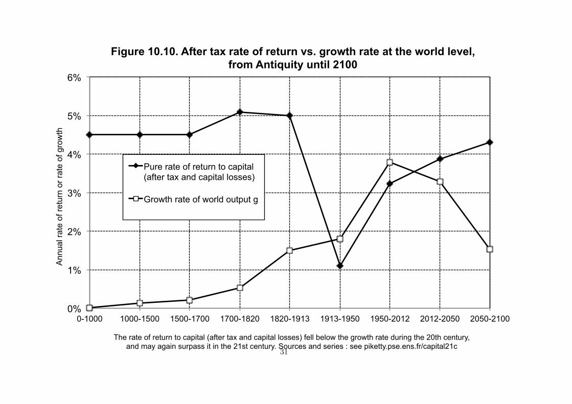
The rate of return to capital (after tax and capital losses) fell below the growth rate during the 20th century, and may again surpass it in the 21st century. Sources and series : see piketty.pse.ens.fr/capital21c

Figure 10.10. After tax rate of return vs. growth rate at the world level, from Antiquity until 2100

Pure rate of return to capital (after tax and capital losses)

Growth rate of world output g

31

0%

1%

2%

3%

4%

5%

6%

0-1000 1000-1500 1500-1700 1700-1820 1820-1913 1913-2012 2012-2100 2100-2200

Ann

ual r

ate

of re

turn

or r

ate

of g

row

th

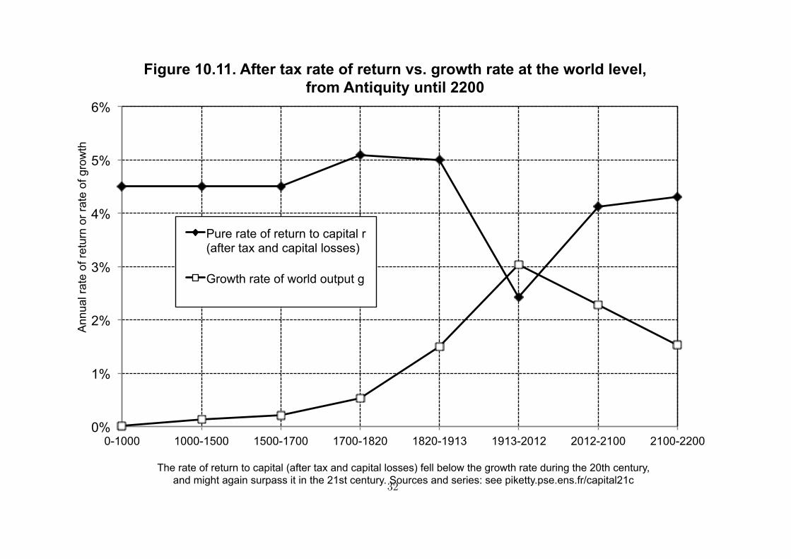
The rate of return to capital (after tax and capital losses) fell below the growth rate during the 20th century, and might again surpass it in the 21st century. Sources and series: see piketty.pse.ens.fr/capital21c

Figure 10.11. After tax rate of return vs. growth rate at the world level, from Antiquity until 2200

Pure rate of return to capital r (after tax and capital losses)

Growth rate of world output g

32

References

Aiyagari S.R. “Uninsured Idiosyncratic Risk and Aggregate Saving”, Quarterly Journal of Economics

1994 (web)

Aiyagari S.R. “Optimal Capital Taxation with Incomplete Markets, Borrowing Constraints, and

Constant Discounting”, Journal of Political Economy 1995 (web)

Alvaredo, Facundo, Anthony B. Atkinson, and Salvatore Morelli, “Top wealth shares in the UK over

more than a century, ” CEPR discussion paper, 2017. (web)

Alvaredo, Facundo, Lucas Chancel, Thomas Piketty, Emmanuel Saez and Gabriel Zucman, “World

Inequality Dynamics: New Findings from WID.world”, American Economic Review P&P May 2017

(web)

Benhabib, J., Bisin, A. and Zhu, S. (2011). “The Distribution of Wealth and Fiscal Policy in

Economies with Finitely-Lived Agents”, Econometrica 2011 (web)

Castaneda A., J. Diaz-Gimenez and J.V. Rios-Rull, “Accounting for the US Earnings and Wealth

Inequality”, Journal of Political Economy 2003 (web)

33

Champernowne D.G. “A Model of Income Distribution”, Economic Journal 1953 (web)

Cowell F., “Inheritance and the Distribution of Wealth”, working paper 1998 (web)

De Nardi, M. and G. Fella, “Saving and Wealth Inequality”, CEPR discussion paper 2017 (web)

Gabaix X., “Power Laws in Economics and Finance”, Annual Review of Economics 2009 (web)

Garbinti, Bertrand, Jonathan Goupille and Thomas Piketty, “Accounting for Wealth Inequality

Dynamics: Methods, Estimates and Simulations for France (1800-2014) ”, working paper, 2017

(web)

Kesten H., “Random difference equations and renewal theory for products of random matrices” Acta

Mathematica 1973

Piketty, Thomas, Capital in the 21st Century, Cambridge: Harvard University Press, 2014 (web)

Piketty, Thomas, and Gabriel Zucman, “Capital is back: wealth-income ratios in rich countries

1700-2010”, Quarterly Journal of Economics, 2014 (web)

Piketty, Thomas, and Gabriel Zucman “Wealth and Inheritance in the Long-Run”,Handbook of Income Distribution, 2015 (web)

34

Piketty, Thomas, Emmanuel Saez, and Gabriel Zucman, “Distributional National Accounts: Methods

and Estimates for the United States”, NBER working paper, 2016 (web)

Saez, Emmanuel, and Gabriel Zucman, “Wealth Inequality in the United States since 1913: Evidence

from Capitalized Income Tax Returns”, Quarterly Journal of Economics, 2016 (web)

Stiglitz J.E. “Distribution of Income and Wealth Amont Individuals”, Econometrica 1969 (web)

35