Eco-efficiency and eco-productivity change over time in a multisectoral economic system

European Journal of Operational Research 234 (2014) 885–897

Contents lists available at ScienceDirect

European Journal of Operational Research

journal homepage: www.elsevier .com/locate /e jor

Interfaces with Other Disciplines

Eco-efficiency and eco-productivity change over time in a multisectoraleconomic system q

0377-2217/$ - see front matter � 2013 Elsevier B.V. All rights reserved.http://dx.doi.org/10.1016/j.ejor.2013.11.017

q The authors gratefully acknowledge the valuable comments received on earlierversions of this paper from two anonymous reviewers as well as the participants atthe VII North American Productivity Workshop (NAPW 2012) in Houston, the 20thInternational Input–Output Conference in Bratislava, the Asia–Pacific ProductivityConference (APPC 2012) in Bangkok, Annual Meeting of the Austrian EconomicAssociation (NOeG 2013) and Thirteenth European Workshop on Efficiency andProductivity Analysis (EWEPA 2013). The authors also would like to thank theOesterreichischen Nationalbank (OeNB) for funding the project under projectnumber 13802. Sandra Lengauer and Peter Luptacik provided valuable researchassistance. This article is also a part of the research project VEGA 1/0906/12«Technical change, catch-up and ecoefficiency: growth and convergence in EUcountries». The usual disclaimer applies.⇑ Corresponding author. Address: Institute for Industrial Research, Mittersteig

10/4, 1050 Vienna, Austria. Tel.: +43 1 5134411 2040; fax: +43 1 5134411 2099.E-mail address: [email protected] (B. Mahlberg).

Bernhard Mahlberg a,c,⇑, Mikulas Luptacik a,b

a Institute for Industrial Research (IWI), Vienna, Austriab Institute for Economic Policy, University of Economics, Bratislava, Slovakiac Vienna University of Economics and Business (WU), Vienna, Austria

a r t i c l e i n f o

Article history:Received 2 July 2013Accepted 15 November 2013Available online 23 November 2013

Keywords:Data envelopment analysisLuenberger indicatorMulti-objective optimisationNeoclassical growth accounting

a b s t r a c t

We measure eco-efficiency of an economy by means of an augmented Leontief input–output modelextended by constraints for primary inputs. Using a multi-objective optimisation model the eco-effi-ciency frontier of the economy is generated. The results of these multi-objective optimisation problemsdefine eco-efficient virtual decision making units (DMUs). The eco-efficiency is obtained as a solution of adata envelopment analysis (DEA) model with virtual DMUs defining the potential and a DMU describingthe actual performance of the economy. This procedure is then extended to an intertemporal approach inthe spirit of the Luenberger productivity indicator. This indicator permits decomposing eco-productivitychange into eco-efficiency change and eco-technical change. The indicator is then further decompoundedin a way that enables us to examine the contributions of individual production factors, undesirable aswell as desirable outputs to eco-productivity change over time. For illustration purposes the proposedmodel is applied to investigate eco-productivity growth of the Austrian economy.

� 2013 Elsevier B.V. All rights reserved.

1. Introduction

One of the goals of the European Union’s strategy for a smart,sustainable and inclusive growth (the so called Europe 2020) isthe reduction of CO2 emissions by 20% compared to 1990 levels(European Commission, 2010). Since a general aim of the economicpolicy in Europe remains to keep economic growth, a reduction ofair pollution requires an increase of eco-efficiency. In this context,increasing eco-efficiency means decoupling pollution (e.g. CO2

emission) from economic development. Without such a de-linkingthe environmental target cannot be fulfilled. Another goal of Eur-ope 2020 is the increase of energy efficiency which is defined asa reduction of energy consumption. This reduction clearly

implicates also a raise in eco-efficiency. Strengthening eco-effi-ciency has also been identified by the United Nations Industryand Development Organization (UNIDO) as one of the major stra-tegic elements in its work on sustainability. It constituted a Cleanerand Sustainable Production Unit (UNIDO, 2012a) and started anEco-efficiency (Cleaner-Production) Program (UNIDO, 2012b).

The concept of eco-efficiency was first described by Schalteggerand Sturm (1989). They defined eco-efficiency as ratio betweenenvironmental impact added and value added. Eco-efficiency aimsat achieving more goods and service outputs with less resource in-puts as well as less waste and emissions. Eco-efficiency is relatedto sustainability in the sense that the later is a broader notionwhereas the former is a new indicator of economic performance.It differs from sustainability in that it takes into account environ-mental and economic dimensions but does not include social as-pects. Eco-efficiency is a necessary but not a sufficient conditionfor achieving sustainability. Measurement of eco-efficiency isimportant to determine success (economic and environmental),identify and track trends, prioritize actions and ascertain areasfor improvement. Monitoring eco-efficiency on the macro-level isuseful in order to make sustainability accountable.

Like in Korhonen and Luptacik (2004), in this paper it is as-sumed that decision making units (say, countries) want to producedesirable outputs as much as possible and produce minimal unde-sirable outputs (e.g. pollutions) with less inputs. In contrast, usualanalysis of (technical) efficiency defines efficiency as a ratio of aweighted sum of desirable outputs to a weighted sum of inputs,

http://crossmark.crossref.org/dialog/?doi=10.1016/j.ejor.2013.11.017&domain=pdf

http://dx.doi.org/10.1016/j.ejor.2013.11.017

mailto:[email protected]

http://dx.doi.org/10.1016/j.ejor.2013.11.017

http://www.sciencedirect.com/science/journal/03772217

http://www.elsevier.com/locate/ejor

886 B. Mahlberg, M. Luptacik / European Journal of Operational Research 234 (2014) 885–897

and does not take undesirable outputs into consideration. The con-cept of eco-efficiency has the advantage over traditional (technical)efficiency that it considers inputs, desirable outputs and undesir-able outputs in one model and takes economical as well as ecolog-ical aspects simultaneously into account.

The efficiency analysis of any decision making unit (DMU) with-out taking economic as well as ecological issues into account oftenyields erroneous inferences concerning the real health of the DMU.This is precisely because there always exists a trade-off betweeneconomy and environment, and an economy’s performance is notsustainable without a healthy ecological system. Because win–win solutions for economy and ecology seem quite elusive in prac-tice, there arises the concept of trade-offs and efficiency frontiersfor economy. Therefore, there is a need to have a measure of per-formance characterised by an eco-efficiency frontier that aims atproviding efficient solutions in relation to the objective of optimis-ing the goals of economy as well as ecology. That is, DMUs lying onthe eco-efficiency frontier cannot increase the output of economicgoods and services without increasing at least one input or increas-ing waste and emissions. These DMUs are efficient in the sense ofKoopmanns (1951). As is known from the literature (see e.g. Färe,Grosskopf, Lovell, & Pasurka, 1989; Färe & Grosskopf, 1996; Sahoo,Luptacik, & Mahlberg, 2011; Tyteca, 1996, 1997), the nonparamet-ric methodology of data envelopment analysis (DEA) helps esti-mating the eco-efficiency frontier. Particularly in the context ofeco-efficiency analysis, the main challenge is the lack of measureslike market prices for undesirable outputs to be used as weights toaggregate various inputs, desirable outputs and undesirable out-puts. Although various techniques for eco-efficiency measurementhave been presented in the literature, most eco-efficiency mea-sures are either very limited or depend on subjective arbitraryweighting scheme. The technique of DEA endogenously generatesthe most favourable weights that maximise the relative efficiencyof the evaluated DMU in comparison with the maximum attainableefficiency. This means that DEA presents every evaluated DMU inits most favourable environment.

In the paper by Luptacik and Böhm (2010) eco-efficiency of awhole economy is measured by means of an augmented Leontief in-put–output model extended by constraints for primary inputs. Usingmulti-objective optimisation models an eco-efficiency frontier ofthe economy is generated. The solutions of the multi-objective opti-misation problems define eco-efficient virtual decision making units(DMUs). The eco-efficiency of the economy can be obtained as a solu-tion of a DEA model with the virtual DMUs defining the potential anda DMU describing the actual performance of the economy. This mod-el allows us taking into account the interdependences of the sectorsin an economy in eco-efficiency analyses. Furthermore, it permitsestimating eco-efficiency of an economy with respect to its own po-tential and without the need to compare it with other economies –economies that may possess different technologies and varying mu-tual interdependencies due to international trade.

This model, however, is purely static and cannot account foreco-efficiency change (catch-up) or explain changes in eco-tech-nology (frontier shift) over time. One main aim of this study is toextend the static eco-efficiency analysis to an intertemporal set-ting. For this purpose the Luenberger productivity indicator is uti-lised, which was introduced by Chambers, Färe, and Grosskopf(1996). This indicator measures productivity change (PRODCH)and permits decomposing it into change in efficiency (EFFCH) onthe one hand and change in the frontier technology, i.e., technicalchange (TECHCH) on the other.

This measure differs from the more frequently applied Malm-quist productivity index in two primary ways. Firstly, it is con-structed based on directional distance functions, whichsimultaneously adjust outputs and inputs in a direction chosenby the investigator, and, secondly, it has an additive structure, i.e.

it is expressed as differences rather than ratios of distance func-tions. Contrary to several other indexes and indicators applied inproductivity studies (e.g. Fisher index, Törnqvist index, Bennet–Bowley indicator) the proposed measure does not demand priceinformation at any stage.

The Luenberger indicator itself is not capable of attributing eco-productivity change to changes in use of production factors or inproduction of undesirable or desirable outputs. To overcome thislimitation our indicator is decomposed in a way that enables oneto examine the contributions of individual production factors andindividual (desirable and undesirable) outputs to eco-productivitychange. The results allow the inference of which inputs and/ordesirable/undesirable outputs of an economy are the drivers ofeco-productivity change.

Our paper is structured as follows. Section 2 presents in detailthe (static) model of Luptacik and Böhm (2010) and extends thismodel in line with the directional distance function approach.Section 3 introduces our method to measure eco-efficiency andeco-productivity change over time; whilst Section 4 deals withan illustrative empirical application of the proposed model, withSection 5 left for our concluding remarks.

2. Methodology

2.1. The augmented Leontief input–output model

The conventional Leontief’s input–output model convenientlydescribes the production relations of an economy in period t fora given nonnegative vector of final demand for n goods producedin n interrelated sectors; gross output of the sectors in period t isdenoted by a n-dimensional vector. Production technology in per-iod t is given by a (n � n) input coefficient matrix. This in turn in-forms the use of a particular good i required for the production of aunit of good j. Luptacik and Böhm (2010) introduced a restriction ofthe use of primary input factors by the available primary inputquantities in period t in this model.

The conventional Leontief’s input–output model has been ex-tended to a model version including pollution generation andabatement activities. The well known augmented Leontief model(Leontief, 1970; see also Lowe (1979), Luptacik & Böhm (1999), &Miller & Blair (2009)) is written as

I � A11;t �A12;t

�A21;t I � A22;t

� �x1;t

x2;t

� �P

y1;t

�y2;t

" #ð1Þ

where the following notation is used: x1,t is the n-dimensional vec-tor of gross industrial outputs in period t; x2,t is the o-dimensionalvector of anti-pollution activity levels in period t; A11,t is the(n � n) matrix of conventional input coefficients (including compet-itive imports), showing the input of good i per unit of the output ofgood j (produced by sector j) in period t; A12,t is the (n � o) matrixwith aik,t representing the input of good i per unit of the eliminatedpollutant k (eliminated by anti-pollution activity k) in period t; A21,t

is the (o � n) matrix showing the output of pollutant k per unit ofgood i (produced by sector i) in period t; A22,t is the (o � o) matrixshowing the output of pollutant k per unit of eliminated pollutantl (eliminated by anti-pollution activity l) in period t; I is the identitymatrix; y1,t is the n-dimensional vector of final demands (reducedby the vector of competitive inputs) for economic commodities inperiod t (also referred to as net output or desirable output); y2,t isthe o-dimensional vector of the net generation of pollutants in per-iod t which remain untreated after abatement activity (also referredto as tolerated level of net pollution or undesirable output). The k-thelement of this vector represents the pollution standard of pollutantk and indicates the tolerated level of net pollution.

B. Mahlberg, M. Luptacik / European Journal of Operational Research 234 (2014) 885–897 887

The first set of equations in (1) describes the use of the pro-duced commodities similar to the traditional Leontief model.The total amount of production should cover the intermediateconsumption, inputs used for the abatement activities, and finaldemand. The second set of equations describes the material bal-ance condition for pollutants. From the total amount of emissiongenerated in the economy one part is eliminated by abatementactivities and one part remains untreated as a tolerated level ofpollution (according to the principle ‘‘what goes in must comeout’’).

The restriction of the use of primary input factors by the avail-able primary input quantities in the augmented model can be writ-ten as

B1;t B2;t½ �x1;t

x2;t

� �6 zt ð2Þ

The relation for primary inputs contains B1,t the (m � n) matrixof primary factor requirements (e.g. labour, capital, non-competi-tive imports, etc.) per unit of gross output in period t for produc-tion activities in period t, B2,t the (m � o) matrix of primary inputcoefficients for abatement activities in period t, and available pri-mary input quantities zt in period t.

In order to model multiple-output multiple-input technolo-gies, the notion of input and output distance functions can beused. For a single output this corresponds to the concept of a pro-duction function. Distance functions are well suited to define in-put and output oriented measures of eco-efficiency. To work outsuch eco-efficiency measures and to derive the output potentialof an economy with n outputs we face in principle a multi-objec-tive optimisation problem. In many cases such problems are re-duced to a single objective optimisation problem by suitableaggregation. For example, ten Raa (1995, 2005) uses world mar-ket prices for the n commodities employed in his model to reducethe optimisation of n outputs to that of a single sum of values ofthe net products.

Pursuing the multiple objective approach and in analogy to Lup-tacik and Böhm (2010) we consider the multi-objective optimisa-tion problem where the net output y1,t is maximised subject torestraints on the availability of primary inputs z0

t as follows

Maxx

y1;t

s:t:ðI � A11;tÞx1;t � A12;tx2;t � y1;t P 0

� A21;tx1;t þ ðI � A22;tÞx2;t þ y2;t P 0

B1;tx1;t þ B2;tx2;t 6 z0t

x1;t; x2;t ; y1;t ; y2;t P 0

ð3Þ

We use the notation ‘‘Max’’ for a vector optimisation problemand ‘‘max’’ for a single objective problem. In order to generate effi-cient units in the sense of Koopmanns (1951) which borders theproduction possibility set, we solve n single objective problemsmaximising final demand for each commodity separately:

max yj1;tðj ¼ 1; . . . ;nÞ ð4Þ

subject to the constraints in (3).For each of the n solutions of (4) denote the (also n-dimen-

sional) solution vector x�jt ðj ¼ 1; . . . ;nÞ representing the gross pro-ductions of commodities. The respective net output columnvectors are denoted y�j1;t . Minimisation of net pollution under theconstraints (3) yields the trivial solution where all variables arezero.

Alternatively for given final demand y01;t and environmental

standard y02;t (the tolerated level of net pollution) the inputs zt

are minimised.

Minx

zt

s:t:

ðI � A11;tÞx1;t � A12;tx2;t P y01;t

� A21;tx1;t þ ðI � A22;tÞx2;t P �y02;t

B1;tx1;t þ B2;tx2;t � zt 6 0x1;t; x2;t ; zt P 0

ð5Þ

In this case, therefore, m single objective problems are solved

min zitði ¼ 1; . . . ;mÞ ð6Þ

subject to the constraints in (5).The m solution vectors x�it ði ¼ 1; . . . ;mÞ describe the optimal

gross production values of commodities for given final demandy0

1;t and environmental standards y02;t under the individual minimi-

sation of the primary factors i = 1, . . . , m. The optimal primary in-put vectors are denoted by z�it .

Like Luptacik and Böhm (2010) these sets of values of bothproblems defined above are arranged column-wise in a pay-off ma-trix with the optimal values appearing in the main diagonal whilethe off-diagonal elements provide the levels of other sectors’ netoutputs and inputs compatible with the individually optimisedones. This pay-off matrix of dimension (n + o + m) � (n + m) forthe augmented model is written in the following way

Qt;t

Zt;t

� �¼

y�11;t � � � y�n1;t

y12;t � � � yn

2;t

z0t � s1

z � � � z0t � sn

z

y01;t þ s1

y1� � � y0

1;t þ smy1

y02;t � s1

y2� � � y0

2;t � smy2

z�1t � � � z�mt

��375

264 �

Q 1;t;t

Q 2;t;t

Zt;t

264

375

where the sijðj ¼ y1; y2; zÞ represent the respective vectors of slack

variables in the optimisation of variable i (i = 1, . . . , n,n + 1, . . . , n + m). Thus, each column of the pay-off matrix contain-ing either the maximal net output of a particular commodity for gi-ven tolerated levels of net pollution and for given inputs (the first ncolumns), or the minimal primary input for given tolerated valuesof net pollution and for given final demand (the last m columns)yields an efficient solution (in the sense of Koopmanns (1951)). Inthis way the eco-efficiency frontier of the economic system canbe generated. In other words, the matrix Qt,t includes the combina-tions of net output quantities that are possible to produce for giventolerated levels of net pollution and for any given combination ofinputs. In this way the ‘‘macroeconomic production function’’ formultiple-input multiple-output technologies can be described.

Each of the points in the pay-off matrix Qt,t is constructedindependently of the other points, but takes account of the entiresystems relations. Knowing the eco-efficiency frontier the eco-efficiency of the actual economy can be estimated. Each of the col-umns of the pay-off matrix can be seen as a virtual decision makingunit with different input and output characteristics which is usingthe same production technique. The real economy as given byactual output and input data defines a new decision making unitwhose distance to the frontier can be estimated.

For this purpose Luptacik and Böhm (2010) formulate the fol-lowing input-oriented DEA model, measuring the eco-efficiencyof the economy described by the actual output and input data

y01;t ; y

02;t ; z

0t

� �min

lh

s:t:

Q1;t;tl P y01;t

� Q 2;t;tl P �y02;t

hz0t � Zt;tl P 0

h;l P 0

ð7Þ


where Q1;t,t is the output matrix, Q2;t,t the pollution matrix, Zt,t theinput matrix, h eco-efficiency and l the intensity vector. The col-umns of the matrix Qt,t are the virtual DMUs, which represent thepoints of the eco-efficiency frontier. DMU0 described by the actual

output and input data y01;t; y

02;t ; z

0t

� �is not included in the descrip-

tion of the production possibility set, this is because the eco-effi-cient points (the virtual DMUs) that enter into the evaluation areunaffected by such a removal. This is also true for an eco-efficientDMU0 that is on a part of the eco-efficiency frontier, but not an ex-treme point.

1 Model (9) and model (10) can be formulated as input-oriented by equating thedirection vector of net outputs with 0 or as output-oriented model by equating thedirection vectors of primary inputs with 0. For oriented models all statements ofthe rest of this section pertain analogously.

2 Apart from using undesirable outputs as inputs several other ways of treatingundesirable outputs are proposed in the literature. A recently published study bySahoo et al. (2011) provides a comprehensive overview.

3 For the condition of the workability of Leontief systems and the notion ofindecomposability of At see e.g. Nikaido (1968).

2.2. The relationship between the DEA model and the LP-Leontiefmodel

Like in Luptacik and Böhm (2010) the augmented Leontief mod-el (2) can alternatively be formulated as an LP-problem by mini-mising primary inputs for given levels of final demand y0

1;t andenvironmental standards y0

2;t we get

minx

c

s:t:

ðI � A11;tÞx1;t � A12;tx2;t P y01;t

� A21;tx1;t þ ðI � A22;tÞx2;t P �y02;t

cz0t � B1;tx1;t � B2;tx2;t P 0

x1;t ; x2;t; c P 0

ð8Þ

The parameter c provides a radial eco-efficiency measure. It recordsthe degree by which primary inputs could be proportionally re-duced but still capable of producing the required net outputs to sat-isfy the exogenously given final demand.

We rephrase the input-oriented eco-efficiency models (7) and(8) taken from Luptacik and Böhm (2010) to models of non-ori-ented proportional directional distance function of eco-efficiencyin the following way:

qt z0t ; y

01;t ; y

02;t

� �¼max

l;bb

s:t:

� by01;t þ Q 1;t;tl P y0

1;t

Q 2;t;tl 6 y02;t

bz0t þ Zt;tl 6 z0

t

l P 0; b free

ð9Þ

and

xt z0t ; y

01;t; y

02;t

� �¼max

x;dd

s:t:

� dy01;t þ ðI � A11;tÞx1;t � A12;tx2;t P y0

1;t

A21;tx1;t � ðI � A22;tÞx2;t 6 y02;t

dz0t þ B1;tx1;t þ B2;tx2;t 6 z0

t

x1;t; x2;t P 0; d free

ð10Þ

The models (9) and (10) are based on the directional distancefunction which was proposed by Chambers, Chung, and Färe(1996) and Chambers, Chung, and Färe (1998). In models (9) and(10) we consider a special case postulating constant returns toscale (CRS). The direction vector for net outputs is equal to theexogenously given level of final demand and for primary inputsequal to the exogenously given level of available inputs,which yields us a non-oriented proportional measure of eco-inefficiency. This is a radial measure which considers the propor-

tional reductions in primary inputs and proportional extension ofdesirable outputs simultaneously.1 The optimal values of models(9) and (10), i.e., qt and -t represent the eco-inefficiency scores ofan economy. For an eco-efficient economy qt = 0 and -t = 0 and foran eco-inefficient economy qt > 0 and -t > 0.

Our approach treats undesirable outputs as inputs. A basic pre-mise of this formulation is based on the economic argument thatboth inputs and undesirable outputs incur costs for firms as wellas whole economies since for abatement purposes in compliancewith the environmental regulations the diversion of productive in-puts from the production of desirable outputs is required. Hence,firms as well as whole economies are usually interested in decreas-ing both as much as possible (cf. Cropper & Oates, 1992). The liter-ature on environmental DEA modelling that treats undesirableoutputs as inputs includes, among others, Hailu and Veeman(2001), Dyckhoff and Allen (2001), Sarkis and Cordeiro (2001),Lee, Park, and Kim (2002), Korhonen and Luptacik (2004), and Yangand Pollitt (2009).2 In our model the tolerated level of net pollutiony0

2;t is determined exogenously by environmental regulation or polit-ical authorities. The modification of undesirable outputs is taken intoaccount by involving abatement activities in the Leontief input–out-put model instead of reducing within the DEA estimator.

Taking into account the interpretation of the eco-inefficiencyparameters b in the DEA model (9) and d in the Leontief model(10) it can be seen that despite the different model formulationsthe objective functions are similar. Both models measure the eco-efficiency of the economy by radial reduction of primary inputs aswell as radial expansion of net output for given amounts of re-sources and final demand in the economy. Denoting

A11;t A12;t

A21;t A22;t

� �¼ At;

y1;t

�y2;t

" #¼ yt and B1;t B2;t½ � ¼ Bt

The relationships between (9) and (10) are given by the follow-ing proposition.

Proposition 1. Assuming the workability of the Leontief system andthe indecomposability3 of the input coefficient matrix A11,t are fulfilledthe eco-inefficiency score qt of DEA problem (9) is exactly equal to theeco-inefficiency measure -t of LP-model (10). The dual solution ofmodel (10) coincides with the solution of the DEA multiplier problem(which is the dual of problem (9)).

Proof. We start with the dual problem to (10).

min p0t;ty0t þ r0t;tz

0t

s:t:p0t;tðI � AtÞ þ r0t;tBt P 0

� p01;t;ty01;t þ r0t;tz

0t ¼ 1

p1;t;t 6 0; p2;t;t P 0; rt;t P 0

ð11Þ

where p0t;t ¼ p01;t;t; p02;t;t

� �with p01;t;t the (1 � n) vector shadow prices

of commodities, p02;t;t the (1 � o) vector of shadow prices for abatingpollutants, and r0t;t the (1 � m) vector of shadow prices of the pri-mary inputs. Because of the indecomposability of A11,t it follows


for the Leontief model that, for y0t P 0; xt > 0 and (I � At)�1 > 0 (cf.

e.g. Nikaido, 1968).Multiplying the augmented Leontief inverse by Qt,t we obtain

the gross production vectors augmented by the anti-pollutionactivity levels corresponding to the individually optimal outputsand primary inputs.

ðI � AtÞ�1Q t;t ¼ T P 0

The total primary inputs required by maximised outputs aregiven by

BtT ¼ Zt;t

The multiplier DEA model (dual model to (9)) is

min u0t;ty0t þ v 0t;tz

0t

s:t:u0t;tQ t;t þ v 0t;tZt;t P 0

� u01;t;ty01;t þ v 0t;tz0

t ¼ 1

u1;t;t 6 0;u2;t;t P 0;v t;t P 0

ð12Þ

where u0t;t ¼ u01;t;t; u02;t;t

� �with u01;t;t the (1 � n) vector shadow prices

of commodities, u02;t;t the (1 � o) vector shadow prices for abatingpollutants, and v 0t;t the (1 � m) vector of shadow prices of the pri-mary input factors.

Substituting (I � At)T = Qt,t and BtT = Zt,t in the first constraint of(12) and multiplying the first constraint of (11) by T yields

u0t;tðI � AtÞT þ v 0t;tBtT P 0

and

p0t;tðI � AtÞT þ r0t;tBtT P 0

Obviously, the first constraints of the problems (12) and (11) are thesame.

Since p0t;ty0t ¼ u0t;ty

0t and r0t;tz

0t ¼ v 0t;tz0

t the dual solutions coincidep0t;t ¼ u0t;t , r0t;t ¼ v 0t;t and the eco-inefficiency scores as well. h

4 Eco-productivity change can also be estimated by applying Malmquist produc-tivity index (e.g. Mahlberg, Luptacik, & Sahoo, 2011) or Malmqust–Luenbergerproductivity index (e.g. Chung, Färe, & Grosskopf, 1997). Both indices allowdecomposing eco-productivity change into eco-efficiency and eco-technical changesimilarly to our approach. Recently, Aparicio, Pastor, and Zofío (2013) proposed asolution of inconsistency of the Malmquist–Luenberger index.

3. Eco-efficiency and eco-productivity change of the economyover time

The main aim of the paper is to analyse the eco-productivitychange of an economy over time and to identify the main driversof this change. For this purpose, following Chambers, Färe et al.(1996), we define the non-oriented proportional Luenberger pro-ductivity indicator over two accounting periods (t and t + 1) as:

PRODCH z0t ; y

01;t ; y

02;t ; z0

tþ1; y01;tþ1; y

02;tþ1

� �¼ 1

2qtþ1 z0

t ; y01;t ; y

02;t

� ��h�qtþ1 z0

tþ1; y01;tþ1; y

02;tþ1

� ��qt z0

t ; y01;t ; y

02;t

� �� qt z0

tþ1; y01;tþ1; y

02;tþ1

� �� ið13Þ

Färe, Grosskopf, and Margaritis (2008) showed that in the spe-cial case of single output, constant returns to scale, and Hicks neu-trality, the Luenberger productivity indicator is equivalent to theSolow specification of technical change. The non-oriented propor-tional Luenberger indicator of eco-productivity change can bedecomposed into eco-efficiency change (catch-up, EFFCH) andeco-technical change (frontier shift, TECHCH) as follows:

EFFCH z0t ; y

01;t ; y

02;t ; z0

tþ1; y01;tþ1; y

02;tþ1

� �¼ qt z0

t ; y01;t ; y

02;t

� �� qtþ1 z0

tþ1; y01;tþ1; y

02;tþ1

� �ð14Þ

TECHCH z0t ; y

01;t ; y

02;t ; z0

tþ1; y01;tþ1; y

02;tþ1

� �¼ 1

2qtþ1 z0

tþ1; y01;tþ1; y

02;tþ1

� ��h�qt z0

tþ1; y01;tþ1; y

02;tþ1

� ��qtþ1 z0

t ; y01;t ; y

02;t

� �� qt z0

t ; y01;t ; y

02;t

� �� ið15Þ

This Luenberger indicator is expressed as the sum of EFFCH andTECHCH. EFFCH captures the average gain/loss in primary inputsand net outputs due to a difference in eco-inefficiency from periodt to period t + 1. TECHCH captures the average gain/loss in primaryinputs and net outputs due to a shift in technology from period t toperiod t + 1.4

To compute the non-oriented proportional Luenberger indicatorand its components, besides the estimation of two own-period eco-

inefficiency scores, i.e. qt z0t ; y

01;t ; y

02;t

� �and qtþ1 x0

tþ1; y01;tþ1; y

02;tþ1

� �,

we need the estimation of two cross-period eco-inefficiency scores:

(1) qtþ1 z0t ; y

01;t ; y

02;t

� �, which represents the degree of eco-ineffi-

ciency of an economy operating at t when evaluated withrespect to the technology at t + 1; and

(2) qt z0tþ1; y

01;tþ1; y

02;tþ1

� �, which represents the degree of eco-

inefficiency of an economy at t + 1 when evaluated with

respect to the technology at t.

First, the linear programming (LP) program in (9) is solved for

two periods (t and t + 1) to arrive at qt z0t ; y

01;t ; y

02;t

� �and

qtþ1 z0tþ1; y

01;tþ1; y

02;tþ1

� �. For these LPs, separate output matrices Q1,

i.e. Q1;t,t and Q1;t+1,t+1, separate pollution matrices Q2, i.e. Q2;t,t

and Q2;t+1,t+1, and separate primary input matrices Z, i.e. Zt,t andZt+1,t+1, have to be constructed by solving the LPs (4) and (6) foreach period.

Second, the cross-period distance function, qtþ1 z0t ; y

01;t ; y

02;t

� �can

be set up as

qtþ1 z0t ; y

01;t; y

02;t

� �¼ max

l;bb

s:t:

� by0t þ Q1;tþ1;tl P y0

1;t

Q 2;tþ1;tl 6 y02;t

bz0t þ Ztþ1;tl 6 z0

t

l P 0; b free

ð16Þ

Similarly, the other cross-period distance function,qt x0

tþ1; y01;tþ1; y

02;tþ1

� �can be set up as

qt z0tþ1; y

01;tþ1; y

02;tþ1

� �¼max

l;bb

s:t:

� by0tþ1 þ Q 1;t;tþ1l P y0

1;tþ1

Q 2;t;tþ1l 6 y02;tþ1

bz0tþ1 þ Zt;tþ1l 6 z0

tþ1

l P 0; b free

ð17Þ

For these two DEA models separate output matrices Q1, i.e.Q1;t+1,t and Q1;t,t+1, separate pollution matrices Q2, i.e. Q2;t+1,t andQ2;t,t+1, and separate primary input matrices Z, i.e. Zt+1,t and Zt,t+1,have to be constructed by solving the LPs (4) and (6). For thesecomputations, production technology on the one hand and avail-able primary input as well as final demand and net pollution onthe other are observed in different periods, which are indicatedby the subscripts t + 1,t and t,t + 1. In total, the LPs (4) and (6) haveto be solved four times.


In the case of the cross-period LP programs, qtþ1 z0t ; y

01;t; y

02;t

� �in

(16) and qt z0tþ1; y

01;tþ1; y

02;tþ1

� �in (17), when the economy under

evaluation remains outside the technology set it is considered‘super eco-efficient’, meaning the eco-inefficiency score b becomesnegative. Such an eco-inefficiency score implies that the primaryinputs need to be increased and net outputs need to be decreasedto get such super eco-efficient economies projected onto the eco-efficiency frontier.

The proposed method allows the researcher to examine the rea-sons of EFFCH, TECHCH and eco-productivity change (PRODCH). Itattributes the use of individual primary input as well as individualcommodity and individual pollutant to eco-productivity changeand its components. To show this we start first by deriving the for-mula for EFFCH, before we present the formulae for TECHCH andPRODCH.

The starting points of this analysis are the definition (14) andthe dual to the DEA model (9) as it is shown in model (12). Aftera few steps of rewriting (see Appendix A) it turns out that the con-tribution of the ith primary input is

EFFCHi ¼ v i;t;tz0i;t � v i;tþ1;tþ1z0

i;tþ1 ð18Þ

that of the jth commodity

EFFCHj ¼ u1;j;t;ty01;j;t � u1;j;tþ1;tþ1y0

1;j;tþ1 ð19Þ

and that of the kth pollutant

EFFCHk ¼ u2;k;t;ty02;k;t � u2;k;tþ1;tþ1y0

2;k;tþ1 ð20Þ

The aggregate indicator for EFFCH can then be arrived at bysumming up their respective input-specific indicators, the respec-tive commodity specific indicators and the respective pollutantspecific indicators (i.e. EFFCH ¼

Pmi¼1EFFCHi þ

Pnj¼1EFFCHjþPo

k¼1EFFCHk).For TECHCH, our starting points are the definition (15) and the

duals to the DEA models (9), (16) and (17). As a result, the contri-bution of the ith primary input is given by

TECHCHi ¼12

v i;tþ1;tþ1z0i;tþ1 � v i;t;tþ1z0

i;tþ1 þ v i;tþ1;tz0i;t � v i;t;tz0

i;t

� �ð21Þ

that of the jth commodity

TECHCHj ¼12

u1;j;tþ1;tþ1y01;j;tþ1 � u1;j;t;tþ1y0

1;j;tþ1 þ u1;j;tþ1;ty01;j;t � u1;j;t;ty0

1;j;t

� �ð22Þ

and that of the kth pollutant

TECHCHk ¼12

u2;k;tþ1;tþ1y02;j;tþ1 � u2;k;t;tþ1y0

2;k;tþ1 þ u2;k;tþ1;ty02;k;t � u2;k;t;ty0

2;k;t

� �ð23Þ

Again, the aggregate indicator of TECHCH can be achieved bysumming up the contributions of all primary inputs, all commodi-ties and all pollutants (i.e. TECHCH ¼

Pmi¼1TECHCHiþPn

j¼1TECHCHj þPo

k¼1TECHCHk).For PRODCH we begin with the definition (13) and the duals to

the DEA models (9), (16) and (17). Hence, the contribution of theith primary input is given by

PRODCHi ¼12

v i;tþ1;tz0i;t � v i;tþ1;tþ1z0

i;tþ1 þ v i;t;tz0i;t � v i;t;tþ1z0

i;tþ1

� �ð24Þ

that of the jth commodity by

PRODCHj ¼12

u1;j;tþ1;ty01;j;t � u1;j;tþ1;tþ1y0

1;j;tþ1 þ u1;j;t;ty01;j;t � u1;j;t;tþ1y0

1;j;tþ1

� �ð25Þ

and that of the kth pollutant by

PRODCHk ¼12

u2;k;tþ1;ty02;j;t � u2;k;tþ1;tþ1y0

2;j;tþ1 þ u2;k;t;ty02;k;t � u2;k;t;tþ1y0

2;k;tþ1

� �ð26Þ

The sum of the contributions of all primary inputs, all commod-ities and all pollutants is exactly equal to PRODCH (i.e.PRODCH ¼

Pmi¼1PRODCHi þ

Pnj¼1PRODCHj þ

Pok¼1PRODCHk).

It can be shown that the contribution of the ith primary input toEFFCH plus the contribution of the ith primary input to TECHCH isequal to the contribution of the ith primary input to PRODCH (i.e.PRODCHi = EFFCHi + TECHCHi). Furthermore, the contribution ofthe jth commodity to EFFCH plus the contribution of the jth com-modity to TECHCH is equal to the contribution of the jth commod-ity to PRODCH (i.e. PRODCHj = EFFCHj + TECHCHj). Finally, thecontribution of the kth pollutant to EFFCH plus the contributionof the kth pollutant to TECHCH is equal to the contribution of thekth pollutant to PRODCH (i.e. PRODCHk = EFFCHk + TECHCHk).

This decomposition enables the researcher to empirically exam-ine the contributions of each individual primary input, individualcommodity and individual pollutant towards the eco-productivitychange and its components – eco-efficiency change and eco-tech-nical change. Since the same inefficiency measure b is used foradjusting inputs as well as desirable outputs the following propo-sition can be proved.

Proposition 2. The total contribution of the primary inputs z0 is equalto the total contribution of all commodities (desirable outputs) y0

1. Thisholds for PRODCH as well as for both components EFFCH and TECHCH.

We show this for EFFCH. For PRODCH and TECHCH the relation-ship can be shown in an analogue way.

EFFCH ¼ qt z0t ; y

01;t ; y

02;t

� �� qtþ1 z0

tþ1; y01;tþ1; y

02;tþ1

� �¼ u01;t;ty

01;t þ u02;t;ty

02;t þ v 0t;tz

0t

� �� u01;tþ1;tþ1y0

1;tþ1 þ u02;tþ1;tþ1y02;tþ1 þ v 0tþ1;tþ1z0

tþ1

� �¼ v 0t;tz

0t � v 0tþ1;tþ1z0

tþ1 þ u01;t;ty01;t � u01;tþ1;tþ1y0

1;tþ1

þ u02;t;ty02;t � u02;tþ1;tþ1y0

2;tþ1 ð27Þ

v 0t;tz0t � v 0tþ1;tþ1z0

tþ1 is the total contribution of all primary inputs andu01;t;ty

01;t � u01;tþ1;tþ1y0

1;tþ1 the total contribution of all commodities andu02;t;ty

02;t � u02;tþ1;tþ1y0

2;tþ1 the total contribution of all pollutants. It hasto be shown that v 0t;tz0

t � v 0tþ1;tþ1z0tþ1 ¼ u01;t;ty

01;t � u01;tþ1;tþ1y0

1;tþ1. Aftera short transformation of the last expression we obtain�u01;t;ty

01;t þ v 0t;tz0

t ¼ �u01;tþ1;tþ1y01;tþ1 þ v 0tþ1;tþ1z0

tþ1. From (12) we knowthat �u0t;ty

01;t þ v 0t;tz0

t ¼ 1 and �u0tþ1;tþ1y01;tþ1 þ v 0tþ1;tþ1z0

tþ1 ¼ 1 whichcomplete the proof.

4. An illustrative empirical application

In this section, we describe how our model can be used to esti-mate eco-productivity growth in Austria, in order to demonstratethe applicability of our proposed approach. In order to investigatetheir importance for eco-productivity growth, we compute thecontributions of different primary inputs, pollutants (undesirableoutputs) and commodities (desirable outputs).

4.1. Dataset

Our data set comprises the two most important primary inputs:labour and capital. Labour is subdivided into three categories: high-skilled, medium-skilled and low-skilled. These are classifiedaccording to the International Standard Classification of Education(ISCED). Thus, high-skilled labour is defined as workers whocompleted the first or also second phase of tertiary education(levels 5–6); medium-skilled as workers who completed uppersecondary education or postsecondary not tertiary education

8 According to the definition of United Nations SNA system of national accounts(United Nations, 2009) the economically active population or labour force comprisesall persons who supply labour for the production of economic goods and services,during a specified time reference period. It equals the sum of the employed and theunemployed.

9 In Austria these are normally 1785.18 hours a year. Following Ortner and Ortner(2012, p. 192) we calculate this as follows: The monthly working hours for a full timeemployed worker are 173.00 hours (Section 3 subparagraph 1 Arbeitszeitgesetz (Working


(levels 3–4) and low-skilled as workers who completed lower sec-ondary education or less (levels 0–2).5 The data source of labourused is Socio-Economic Accounts of the World Input–Output Data-base (WIOD). Labour is measured in millions of hours worked. Thetime series were downloaded in July 2012. Capital is representedby total net fixed assets at replacement prices of 2005 and containsall asset types – including crop plants, kits, vehicles, residentialbuildings, other types of buildings, intangible assets. It is taken fromStatistics Austria and measured in billions of EUR. The capital stockactually used cannot be observed directly and has to be estimated.This estimation is done by multiplying data on fixed capital stock ta-ken from Statistics Austria6 by capacity utilisation rate for totalindustry taken from Eurostat. Hence, our empirical model consistsof four primary inputs: labour of three skill types, and capital. Thesedata serve as a basis for computation of the matrices of primary in-put requirement per unit of gross output for production activities(B1-matrices) of the respective years. In our empirical applicationwe cover an observation period from 1995 to 2007.

Since our model is based on an augmented Leontief model, dataon environmental workers are required. As these data are not avail-able from any data source they have to be estimated. In a first stepwe compute the share of labour compensation paid for environmen-tal protection (section ambient air and climate) on total labour com-pensation for industry and construction sectors. In a second step wemultiply this share with the total number of employees to get theestimated total number of environmental workers. Finally, we dis-tribute the total number to the three levels of three skill-levels andconvert in million hours worked. Data on labour compensationand total number of employees are taken from Austrian EconomicChamber (1998, 1999) and Statistics Austria (2008a, 2008b). In addi-tion, data on environmental capital stock are required. These data arenot available from any data source and has to be estimated as well.This estimation is done by applying the perpetual inventory methodbased on time series of gross fixed capital formation for environmen-tal protection from Austrian Economic Chamber (until the year2002) and Statistics Austria (from the year 2002 on). Data on envi-ronmental workers and environmental capital stock are used forcomputation of the matrix of primary input coefficients for abate-ment activities (B2-matrices) of the respective years.

The interrelationships between the commodities are measured byinput–output tables that are usually provided in two versions: a ver-sion which includes domestic inputs as well as imported inputs (so-called ‘‘version A’’) and a version which contains domestic inputs only(so-called ‘‘version B’’). Due to the availability of data and because ofthe illustration purpose of this empirical application the version B ofAustrian input–output tables is used. For the analysis of the develop-ment of the Austrian economy with the aim to derive conclusions forthe economic policy the version A should be used. The input–outputtables for 1995 (Statistics Austria, 2001) and 2007 (Statistics Austria,2011a) are deflated to price level of 2005 by applying the approachdeveloped by Dietzenbacher and Hoen (1998) and Koller and Stehrer(2010) in order to exclude changes of the A-matrices due to the changeof relative prices. Because our analyses are done mainly for illustrationpurposes we content ourselves with rather highly aggregated input–output tables. The tables are aggregated to eighteen times eighteen7

by applying the approach of Olsen (2000, 2001) (see also Kymn(1990) and Kymn & Norsworthy (1976) for comprehensive surveys ofaggregation approaches). From these input–output tables the conven-tional domestic input coefficient matrices (A11-matrices) are computed.

5 The end of level 2 often coincides with the end of compulsory schooling.6 We consider the fixed capital stock provided by Statistics Austria as capital

endowment and not as capital actually used.7 The input–output tables are aggregated in accordance with the availability and

structure of the pollution abatement and air emission data provided by StatisticsAustria.

We augment the conventional input–output tables by addingpollution abatement for climate protection and pollution control andair emissions (sum of SO2, NOX, NMVOC, CH4, CO, CO2, N2O, NH3

and PM10). These data were obtained from integrated NAMEA (Na-tional Accounting Matrix including Environmental Accounts). For adetailed description see Statistics Austria (2011b). Based on thesedata we compute the matrix of pollution abatement per unit ofeliminated pollutant (A12-matrices) and the matrix showing theoutput of pollutant per unit of gross output (A21-matrices). Sincewe take just one type of pollution (i.e. air emissions) into accountthe respective matrices are one column vector (A12-matrices) andone row vector (A21-matrices). The matrix showing the output ofpollutant per unit of eliminated pollutant (A22-matrices) is just azero in our application.

Final demand for economic commodities (y1-vectors) serves as themeasure of desirable outputs and consists of eighteen aggregatesof commodities. These data are taken from Statistics Austria(2001) and Statistics Austria (2011a) and deflated by applyingthe approach developed by Dietzenbacher and Hoen (1998) andKoller and Stehrer (2010). The tolerated level of net pollution(y2-vectors), which is our measure of undesirable output, is speci-fied as reduction of air emission by 10% of the 1995 level of grossemissions (in the year 1995) and as a decline by 30% of the 1995level of gross emissions (in the year 2007).

The vector of gross industrial outputs (x1-vectors) serving as a basisof the computation of the input requirement matrix of productionactivity (B1-matrices) is taken from the input–output tables. Theanti-pollution activity level (x2-vectors) serving as a basis of the compu-tation of the matrix of primary input coefficients for abatement activ-ities (B2-matrices) is calculated as the difference of the gross pollutionlevel of the respective year minus the tolerated level of net pollution(y2-vectors). Since we take into account just one pollutant (i.e. airemissions) the anti-pollution activity level is just a scalar.

The labour endowment in hours of the Austrian economy can-not be observed directly. Therefore, we have to estimate them byapplying the following procedure. In a first step, we take data onthe population of different skill levels of the respective years fromStatistics Austria (for the year 1995) and Eurostat (for the year2007). We define the working-age population as all persons be-tween 15 and 64 years. These data are given in number of persons.The working-age population cannot be considered as labourendowment in the sense of our model (labour component of thez0-vectors) since it does not measure the economically active pop-ulation or labour force.8 In order to get the right measure of laboursupply we multiply the working-age population with the labourforce participation rate of different skill levels taken from Eurostat.Since our labour used in production is measured in hours workedthe labour supply data given in number of persons need to be con-verted in hours to get suitable data on labour endowment of the Aus-trian economy. We multiply the number of persons by the number ofhours usually worked by a full time employed person during a year.9

Time Act of Austria)). We multiply the monthly working hours by 12 months to get theyearly working hours of 2076.00 hours. From this we subtract hours of not performancetimes due to vacations and due to legal holidays. The number of vacation days are 25working days (Section 2 subparagraph 1 Urlaubsgesetz (Holiday Act of Austria)) and thenumber of legal holidays are 12 days (Section 7 subparagraph 2 Arbeitsruhegesetz (Restfrom Work Act of Austria)). The number of vacation days and the number of legal holidaysare multiplied by 7.86 hours (Ortner & Ortner, 2012, p. 734). The computation in detail isthe following: 2076.00 � (25 + 12) � 7.86 = 1785.18.

Table 1Utilisation of primary inputs.

Resourcesused (1)

Endowment(2)

Utilisation(=(1)/(2))

1995High-skilled labour (in

millions hours)741 767 0.97

Medium-skilled labour (inmillions hours)

3974 4219 0.94

Low-skilled labour (inmillions hours)

1435 1792 0.80

Capital, all assets (in billionsEUR)

597 708 0.84

2007High-skilled labour (in

millions hours)1231 1298 0.95

Medium-skilled labour (inmillions hours)

4305 4687 0.92

Low-skilled labour (inmillions hours)

1255 1421 0.88

Capital, all assets (in billionsEUR)

811 915 0.89


The capital stock endowment data (capital component of the z0-vec-tors) are taken from Statistics Austria.

4.2. Descriptive statistics

This section presents some descriptive statistics. They give afirst impression of the eco-productivity development of Austriaduring the observation period and support the interpretation ofthe estimation results presented in the next section.

Table 1 shows data and utilisation rates of primary inputs. Forhigh and medium-skilled labour as well as capital, the quantitiesused and the endowments clearly increased during the observa-tion period. For low-skilled labour, quantities used and endow-ment clearly decreased. Furthermore, from Table 1 it can beseen that the resource utilisation (i.e. ratio of resources used toresource endowment) of high-skilled and medium-skilled labourworsened, whereas of low-skilled labour as well as of capitalstock improved. These data indicate that the utilisation of thetwo scarcest resources decreased. Based on this development itcan be expected that the eco-efficiency change component ofthe Luenberger indicator will reveal eco-efficiency regress of thewhole economy.

Table 2 presents the data on final demand, tolerated level of netpollution and their growth. It can be seen that the final demand foralmost all commodities increased, and growth rate differs fromcommodity to commodity. The pollution (net air emissions) clearlydecreased due to an active environmental policy.

Table 3 compares structure of final demand in 1995 and 2007.In terms of change in share the commodity Motor vehicles andtransport equipment gained remarkable whereas the commoditiesconstruction work as well as other services and public administra-tion clearly shrank. Overall the final demand for commodities ofthe secondary sector increased more than of the agricultural sectorand the service sector.

Table 4 presents the aggregated primary input requirementmatrices of 1995 and 2007. Input requirement is defined as the ra-tio of amount of primary inputs used in a sector divided by grossoutput of a sector and tells how much of a resource is needed toproduce one unit of gross output. A decrease over time indicatesan increase of the productivity of this factor in the respective sec-tor. In such a case, fewer resources are required to produce oneunit of output. From this table it can be seen that in most sectors,as well as on average, the values of primary input requirements forproduction activities decreased. The development for pollution

abatement was clearly different from that of production activities.The labour requirement per unit of prevented emissions increasedvery much whereas the capital requirement decreased. In spite ofthe decrease of labour productivity of the abatement activities itcan be expected that overall the eco-technical change componentof the Luenberger Indicator will indicate eco-technical progresssince pollution abatement accounts for a relatively small share ofactivities of the Austrian economy. From the estimation results ofthe contributions to eco-technical change we probably will see thatpollution abatement contributes negatively.

Table 5 shows the emission coefficients of 1995 and 2007. Thisindicator measures how much air emissions are generated perunit of gross production. A decrease of these coefficients indicatesenvironmental saving eco-technical progress. Such a develop-ment can be seen from the numbers in Table 5. The values clearlydecreased in all three sectors as well as overall. This data indicatea positive contribution of abatement activities to eco-technology.The net effect of the developments shown in Tables 4 and 5 is apriori unclear and can be seen only from estimations by meansof our model.

4.3. Estimation results

First we compute the eco-inefficiency scores and the shadowprices for the years 1995 and 2007 applying the DEA model [(9)and (12)] and the Leontief model [(10) and (11)] in order to showempirically that the estimation results of both models are equal. Ascan be seen from Table 6, this is indeed the case, and the empiricalresults confirm the statement of Proposition 1. The first line belowthe column heading shows eco-inefficiency scores of 0.0167 and0.0262 in the years 1995 and 2007, respectively. These resultscan be interpreted as follows: in both years the Austrian economyis eco-inefficient, in the sense that its actual performance deviatesfrom its potential and its resources are not fully utilised. In 1995the Austrian economy could increase its actual final demand anddecrease the actual use of primary inputs by round 1.7%, simulta-neously. In 2007, the Austrian economy is even more eco-ineffi-cient, further away from its possibilities, and its potential forimprovement is larger than in 1995. It could raise the actual finaldemand and reduce the primary inputs actually used by around2.6%.

Additionally, Table 6 shows the results of shadow prices com-putations. Positive shadow prices of primary inputs indicate thatan increase in the endowment ceteris paribus raises eco-ineffi-ciency because of the increased difference between the endow-ment and utilised quantities. This is also true for net pollution.An increase in the tolerated level of air emissions (undesirableoutput) ceteris paribus increases eco-inefficiency. Conversely,negative shadow prices of commodities reveal that an increasein final demand (desirable output) ceteris paribus reduces eco-inefficiency. Generally speaking, a non-zero shadow price indi-cates that the respective resource or commodity is scarce, andthe environmental standard for the respective pollutant isrestrictive. By contrast, a value of zero implies that a change inendowment or final demand or net pollution does not changeeco-inefficiency and shows the respective resource or commodityis abundant or the environmental standard for the respective pol-lutant is not restrictive. The results presented in Table 6 indicateclearly that in 1995 as well as in 2007 high-skilled labour isscarce, whereas the other primary inputs are abundant. Thus,only one primary input is scarce. This follows from the assump-tion of the linear programming technology without direct substi-tution possibilities where the value of the objective function (inour model the inefficiency score) is determined by the scarcestresource. An additional unit of high-skilled labour endowment(with all other things held constant) raises eco-inefficiency,

Table 2Descriptive statistics of final demand and pollution.

1995 2007 Growth ratein percent

In billions EUR

Products of agriculture, hunting,forestry and fishing

1.15 1.64 42.48

Mining 0.21 0.65 210.14Food, beverages and tobacco 8.82 10.98 24.54Textiles and leather 3.39 2.84 �16.16Wood and products of wood 2.12 4.36 105.53Paper and printed matter 3.46 5.90 70.40Chemical and refined petroleum products 4.84 9.18 89.74Other non-metallic mineral products 2.29 2.44 6.59Basic metals 4.11 9.47 130.71Machinery and equipment 18.03 31.52 74.76Motor vehicles and transport equipment 5.74 16.46 186.89Other manufactured goods 7.27 10.08 38.73Electrical Energy 2.21 4.28 93.35Construction Work 21.86 23.12 5.79Land transport services 5.35 6.16 15.23Water transport services 0.07 0.06 �17.05Air transport services 0.65 2.10 225.16Other services and public administration 126.59 174.01 37.46

Total 218.14 315.25 44.51In millions tons In percent

Net pollution (i.e. net air emissions) 44.66 34.73 �22.22

Table 3Structure of final demand.

1995 2007 Changein percentagepoints

In percent

Products of agriculture, hunting, forestryand fishing

0.53 0.52 �0.01

Mining 0.10 0.21 0.11Food, beverages and tobacco 4.04 3.48 �0.56Textiles and leather 1.55 0.90 �0.65Wood and products of wood 0.97 1.38 0.41Paper and printed matter 1.59 1.87 0.28Chemical and refined petroleum products 2.22 2.91 0.69Other non-metallic mineral products 1.05 0.77 �0.28Basic metals 1.88 3.00 1.12Machinery and equipment 8.27 10.00 1.73Motor vehicles and transport equipment 2.63 5.22 2.59Other manufactured goods 3.33 3.20 �0.13Electrical Energy 1.01 1.36 0.34Construction Work 10.02 7.33 �2.68Land transport services 2.45 1.95 �0.50Water transport services 0.03 0.02 �0.01Air transport services 0.30 0.67 0.37Other services and public administration 58.03 55.20 �2.83

Table 4Primary input requirement matrices (B-matrices).

Primarysector

Secondarysector

Tertiarysector

Mean Pollutionabatement

1995High-skilled

laboura61.25 12.10 1.73 1.47 0.05

Medium-skilledlaboura

91.83 109.47 10.73 13.57 0.08

Low-skilledlaboura

61.25 39.19 3.19 6.29 0.03

Capital totalb 6,35 10.65 1.81 1.35 0.79

2007High-skilled

laboura9.81 15.98 1.55 1.78 0.13

Medium-skilledlaboura

48.98 69.07 8.17 8.38 0.21

Low-skilledlaboura

22.24 19.97 2.09 2.81 0.08

Capital totalb 5.08 7.85 1.68 1.09 0.25

a In hours worked per 1.000 EUR produced (labour per gross output).b In unity (capital per gross output).

Table 5Emission coefficients 1995 and 2007.

Primarysector

Secondarysector

Tertiarysector

Overall

1995 In tons per 1000EUR

0.360 0.310 0.041 0.152

2007 0.304 0.275 0.038 0.138

Note: weighted averages of commodities.


whereas an increase of all other primary inputs does not changeeco-inefficiency. From 1995 to 2007 the shadow price ofhigh-skilled labour decreases clearly indicating that this type oflabour becomes less scarce. This development corresponds tothe decrease of utilisation of high-skilled labour shown in Table 1.A similar situation can be found for net air emissions (undesir-able output). The shadow price is positive indicating that anincrease of tolerated level of pollution raises eco-inefficiency.Furthermore, according to the shadow prices listed in Table 6an increase in final demand (desirable output) for any commod-ity decreases eco-inefficiency in both years indicating all of themare scarce.

In a next step, we apply our DEA models and the Luenbergerproductivity indicator to estimate the eco-productivity change(PRODCH) in the Austrian economy from 1995 to 2007. The resultsare shown in Table 7. Again, we apply our DEA model as well as theaugmented Leontief model, and compare the results in order to

check whether the outcomes coincide. It turns out that the resultsof both models are exactly the same. The eco-inefficiency scores ofsingle period and mixed period models are equal. As a conse-quence, the values of EFFCH, TECHCH and PRODCH are the sameas well. According to our results, the eco-efficiency of the Austrianeconomy slightly decreases. The EFFCH score is around �0.010indicating eco-efficiency regress of approximately 1%. This out-come confirms our expectations drawn from Table 1 and is plausi-ble against the background of a general increase of unemploymentin Austria during the observation period. Contrary to eco-efficiencyregress, we find a positive TECHCH score of around 0.057 indicatingtechnical progress of 5.7%. This value shows that the Austrianeconomy goes through a clear eco-technical progress during theobservation period. This result confirms our expectations drawnfrom Table 4. By means of the EFFCH scores and TECHCH scoresPRODCH can be easily computed as PRODCH is simply equal tothe sum of EFFCH and TECHCH. This simple procedure yields aPRODCH score of around 0.047 indicating eco-productivity pro-gress of circa 4.7%.

These results raise the question as to which primary input aswell as which commodity cause EFFCH, TECHCH and PRODCH andwhat is the role of pollution. Or in other words, what are thecontributions of the individual inputs as well as desirable andundesirable outputs to eco-efficiency, eco-technology and eco-productivity development. To answer these questions, we applythe approach described in the previous section, i.e. the formulae(18)–(26), which combines shadow prices and observed data(endowment of primary input as well as exogenous given final de-mand for commodities and tolerated level of air emissions) to esti-mate the contributions of individual primary inputs as well asdesirable and undesirable outputs. The results are shown in Table 8.

Table 6Eco-inefficiency scores and shadow prices from single period DEA and augmented Leontief model for 1995 and 2007.

1995 2007

DEA-model Leontief-model DEA-model Leontief-model

Eco-inefficiency scores 0.0167 0.0167 0.0262 0.0262Shadow prices

Final demand Products of agriculture, hunting, forestry and fishing �0.00564 �0.00564 �0.00596 �0.00596Mining �0.00158 �0.00158 �0.00113 �0.00113Food, beverages and tobacco �0.00262 �0.00262 �0.00202 �0.00202Textiles and leather �0.00127 �0.00127 �0.00125 �0.00125Wood and products of wood �0.00238 �0.00238 �0.00185 �0.00185Paper and printed matter �0.00164 �0.00164 �0.00109 �0.00109Chemical and refined petroleum products �0.00107 �0.00107 �0.00063 �0.00063Other non-metallic mineral products �0.00185 �0.00185 �0.00126 �0.00126Basic metals �0.00129 �0.00129 �0.00067 �0.00067Machinery and equipment �0.00150 �0.00150 �0.00098 �0.00098Motor vehicles and transport equipment �0.00099 �0.00099 �0.00055 �0.00055Other manufactured goods �0.00158 �0.00158 �0.00126 �0.00126Electrical Energy �0.00180 �0.00180 �0.00094 �0.00094Construction Work �0.00109 �0.00109 �0.00126 �0.00126Land transport services �0.00210 �0.00210 �0.00144 �0.00144Water transport services �0.00192 �0.00192 �0.00101 �0.00101Air transport services �0.00181 �0.00181 �0.00079 �0.00079Other services and public administration �0.00277 �0.00277 �0.00187 �0.00187

Pollution Air emissions 0.00015 0.00015 0.00004 0.00004Primary inputs Low-skilled labour 0 0 0 0

Medium-skilled labour 0 0 0 0High-skilled labour 0.00066 0.00066 0.00039 0.00039Capital 0 0 0 0

Note: DEA model . . . models (9) and (12), Leontief model . . . models (10) and (11).

Table 7Results of Luenberger Indicator and its components, 1995–2007.

DEA model Leontief model

Eco-inefficiency scoresIn 1995 0.0167 0.0167In 2007 0.0262 0.02621995–2007 (mixed period) �0.1747 �0.17472007–1995 (mixed period) �0.0702 �0.0702

Luenberger indicatorEco-efficiency change (EFFCH) �0.0096 �0.0096Eco-technical change (TECHCH) 0.0570 0.0570Eco-productivity change (PRODCH) 0.0474 0.0474


Note that the column sums are equal to the EFFCH score, TECHCHscore and PRODCH score, respectively.

It turns out that eco-efficiency regress is driven by a decline inutilisation of certain primary inputs as well as insufficient growthof the final demand for certain commodities. Among the primaryinputs high-skilled workers’ contribution to EFFCH is clearly neg-ative. This corresponds to the findings of Table 1 showing a de-crease in utilisation of this resource. Due to the linearity of themodel, the scarcest resource (i.e. high-skilled labour in our case)determines eco-inefficiency scores and therefore eco-efficiencychange results and contributions. The results also reflect thechange in terms of shortage, which can be seen from shadowprices in Table 6. The shadow price of high-skilled labour de-creases from 1995 to 2007 but the endowment increases andconsequently the expenditures increases. Since the contributionof a primary input is the difference between expenditures inthe first year and in the second year (see formula (18)), the con-tribution turns out to be negative. The contributions of the otherthree primary inputs amount to zero as the shadow prices of allof them are equal to zero in both years.

For net air emission Table 8 shows a positive contribution toeco-efficiency change. In Table 2 we see a decrease of quantity

from 1995 to 2007 and in Table 6 a decline of shadow prices. Bothinduce lower expenditures in the second year and consequently in-crease eco-efficiency. Our model indicates that a decrease of toler-ated level of air emissions (i.e. improvement of environmentalstandards) improves eco-efficiency.

The contributions of twelve out of eighteen commodities aresmall and positive. For all of these commodities the economic rev-enue is higher in the first year than in the second year. For almostall of these commodities the growth of final demand is above aver-age (see Table 2) and overcompensats the decrease of shadowprices. For the commodities which contribute negatively thegrowth of final demand is below average. The commodity calledother services and public administration shows the highest nega-tive contribution since its final demand is the largest of all negativecontributing commodities.

Eco-technical progress in the Austrian economy is driven by pri-mary inputs as well as desirable and undesirable outputs. Amongthe primary inputs, high-skilled labour contributes clearly posi-tively whereas low-skilled labour contributes clearly negatively.The positive contribution of the former exceeds the negative oneof the later so as to totally the contribution of labour is positive.This outcome corresponds to the findings of Table 4 showing thatthe production technology becomes more skill-intensive (i.e. morerequirement of high-skilled and less requirement of low-skilled la-bour). The relationship between the contributions of high-skilledand low-skilled labour reflects the well-known substitution be-tween these two production factors. In our model the substationbetween production factors is just indirect caused by the changein final demand and the subsequent change in gross production.Medium-skilled labour and capital do not contribute since itsshadow prices are always zero, showing that they are not scarce re-sources neither in the first year nor in the second. The contribu-tions of final demand for any commodity are marginally positive,with the exception of the clearly negative contribution of otherservices and public administration. The compulsory reduction of

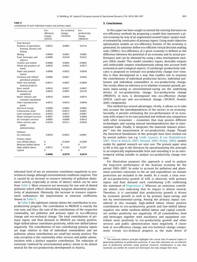
Table 8contribution of each individual output and primary input.

Eco-efficiencychange(EFFCH)

Eco-technicalchange(TECHCH)

Eco-productivitychange(PRODCH)

Final demandProducts of agriculture,

hunting, forestry andfishing

0.0033 0.0085 0.0118

Mining 0.0004 0.0001 0.0005Food, beverages and

tobacco�0.0009 0.0230 0.0222

Textiles and leather �0.0008 0.0003 �0.0005Wood and products of

wood0.0030 0.0042 0.0072

Paper and printedmatter

0.0008 0.0022 0.0030

Chemical and refinedpetroleum products

0.0006 0.0021 0.0026

Other non-metallicmineral products

�0.0012 0.0007 �0.0004

Basic metals 0.0010 0.0037 0.0047Machinery and

equipment0.0039 0.0087 0.0126

Motor vehicles andtransport equipment

0.0034 0.0039 0.0074

Other manufacturedgoods

0.0012 0.0033 0.0044

Electrical energy 0.0000 0.0005 0.0005Construction work 0.0053 �0.0013 0.0041Land transport services �0.0024 0.0017 �0.0007Water transport services �0.0001 0.0000 0.0000Air transport services 0.0005 0.0009 0.0014Other services and

publicadministration

�0.0256 �0.0313 �0.0569

PollutionAir emissions 0.0054 �0.0055 �0.0001

Primary inputsLow-skilled labour 0 �0.2049 �0.2049Medium-skilled labour 0 0 0High-skilled labour �0.0075 0.2362 0.2287Capital 0 0 0

�0.0096 0.0570 0.0474

10 The materials balance principle highlights the crucial role of material inputs ingenerating pollution in production processes. It says that emissions are an inherentpart of production activities using material resources. Furthermore, it says thatmaterials can neither be created nor destroyed, but only change their form.


tolerated level of net air emissions contributes negatively to eco-technical change although environmental conditions improve. Thisis caused by an increase in resource intensity of pollution abate-ment activity (especially in terms of labour) which can be seenfrom Table 4. More resources are necessary for one unit of abatedpollution which reflects diminishing marginal abatement produc-tivity of abatement. Obviously, the increase in resource require-ment outbalances the improvement in emission coefficientsshown in Table 5.

In Table 8 the rightmost column shows the contribution to eco-productivity progress. The contribution to PRODCH is exactly therow sum, and thus, the sum of the contributions of the respectivecommodity, net pollution and primary input to eco-efficiencychange and eco-technical change. The total contributions of pri-mary inputs and final demand to PRODCH are clearly positive.High-skilled labour contributes positively, while low-skilled labournegatively. The contributions of two contributing primary inputsare large relative to that of individual commodities and netpollution, whose contributions are small but mostly positive. Theonly exception is the commodity other services and public admin-istration with a distinct negative contribution. The reduction ofemissions (induced by environmental policy) seems to be almostneutral for the eco-productivity development in Austria.

5. Conclusions

In this paper we have sought to extend the existing literature oneco-efficiency methods by proposing a model that represents a gi-ven economy by way of an augmented Leontief input–output mod-el extended by constraints of primary inputs. Using multi-objectiveoptimisation models an eco-efficiency frontier of the economy isgenerated. Its solutions define eco-efficient virtual decision makingunits (DMUs). Eco-efficiency of a given economy is defined as thedifference between the potential of an economy and its actual per-formance and can be obtained by using a data envelopment anal-ysis (DEA) model. This model considers inputs, desirable outputsand undesirable outputs simultaneously taking into account botheconomical and ecological aspects. A Luenberger productivity indi-cator is proposed to estimate eco-productivity change over time;this is then decomposed in a way that enables one to examinethe contributions of individual production factors, individual pol-lutants and individual commodties to eco-productivity change.The results allow an inference as to whether economic growth, pri-mary input-saving or environmental-saving are the underlyingdrivers of eco-productivity change. Eco-productivity change(PRODCH), in turn, is decomposed into eco-efficiency change(EFFCH, catch-up) and eco-technical change (TECHCH, frontiershift) components.

This method has several advantages. Firstly, it allows us to takeinto account the interdependences of the sectors in an economy.Secondly, it permits estimating the eco-performance of an econ-omy with respect to its own potential and without any comparisonwith other economies – economies that may possess differenttechnologies and varying mutual interdependencies due to inter-national trade. Finally, it integrates the materials balance princi-ple10 into the measurement of eco-productivity change. Thoughthe theoretical foundations of this principle have been worked outby several authors (see e.g. Coelli, Lauwers, & van Huylenbroeck,2007; Ebert & Welsch, 2007; Førsund, 2009; Pethig, 2006), modelsusable for applied research are very rare. The present paper aimsto fill in this gap in the literature by operationalizing this principleto an empirically implementable form and extending it to an inter-temporal setting suitable to analyze eco-productivity change overtime.

For illustration purposes this approach is used to analyzethe long-term performance of the Austrian economy for theperiod 1995–2007. In order to account for pollution and abate-ment activities emissions to the air and expenditure on climateprotection are included in the model. As a result, a clear over-all eco-productivity growth of 4.8% is observed, with primaryinputs and final demand each contributing 2.4% confirmingthe statement of Proposition 2. Whereas air emissions contrib-ute almost zero indicating that its impact is almost neutral.Therefore, it is concluded that productivity growth is drivenby economic growth as well as by primary input-saving, andnot by environmental-saving. Among the primary inputs con-sidered in this example, high-skilled labour shows positivecontribution to eco-productivity growth and low-skilled labournegative one while medium-skilled labour and capital contrib-ute neither positively nor negatively. Of all commodities, foodand beverages together with machinery and equipment con-tribute most positively to eco-productivity growth and otherservices and public administration most negatively. A closerlook at eco-efficiency change and eco-technical change compo-nents reveals eco-technical progress as the main driver of


eco-productivity progress. Eco-technical progress is mostly dri-ven by high-skilled labour whereas low-skilled labour contrib-utes negatively. Conversely, high-skilled labour contributesnegatively to eco-efficiency change caused by the less efficientusage of this resource in 2007 as compared to 1995 owing toincreased unemployment amongst graduates. Air emissionscontribute slightly negatively to eco-technical change. Thisnegative contribution is almost completely compensated by aslightly positive one to eco-efficiency change caused by a gen-eral reduction of air emissions resulting in an almost zero con-tribution to eco-productivity.

Finally, we point to avenues for future research. Firstly, withregard to the empirical part of the paper the model could be ex-tended by additional types of pollutants and further kinds ofabatement activities – depending on data availability – in orderto complete the evaluation of environmental policy measures.Secondly, the proposed model could be a starting point to builda comprehensive model for analysing resource- or energy-effi-ciency and -productivity as a useful tool for investigating the pos-sible impacts of the Europe 2020 goals (European Commission,2010).

Appendix A

The appendix shows the details of the derivation of the contri-butions of individual inputs, pollutants, and commodities to EFFCH,TECHCH and PRODCH.

1. Eco-efficiency change (EFFCH):

EFFCH z0t ;y

01;t ;y

02;t;z

0tþ1;y

01;tþ1;y

02;tþ1

� �¼qt z0

t ;y01;t ;y

02;t

� ��qtþ1 z0

tþ1;y01;tþ1;y

02;tþ1

� �

¼Xn

j¼1

u1;j;t;ty01;j;tþ

Xo

k¼1

u2;k;t;ty02;k;tþ

Xm

i¼1

v i;t;tz0i;t

!

�Xn

j¼1

u1;j;tþ1;tþ1y01;j;tþ1þ

Xo

k¼1

u2;k;tþ1;tþ1y02;k;tþ1þ

Xm

i¼1

v i;tþ1;tþ1z0i;tþ1

!

¼Xn

j¼1

u1;j;t;ty01;j;t�

Xn

j¼1


Xo

k¼1

u2;k;t;ty02;k;t

�Xo

k¼1


Xm

i¼1

v i;t;tz0i;t�

Xm

i¼1


ð28Þ

2. Eco-technical change (TECHCH):

TECHCH z0t ;y

01;t ;y

02;t ;z

0tþ1 ;y

01;tþ1 ;y

02;tþ1

� �

¼12

qtþ1 z0tþ1 ;y

01;tþ1 ;y

02;tþ1

� ��qt z0

tþ1 ;y01;tþ1 ;y

02;tþ1

� �� hþ qtþ1 z0

t ;y01;t ;y

02;t

� ��qt z0

t ;y01;t ;y

02;t

� �� i

¼12

Xn

j¼1


Xo

k¼1


Xm

i¼1


! "

�Xn

j¼1

u1;j;t;tþ1y01;j;tþ1þ

Xo

k¼1

u1;k;t;tþ1y01;k;tþ1þ

Xm

i¼1

v i;t;tþ1z0i;tþ1

!!

þXn

j¼1

u1;j;tþ1;t y01;j;t þ

Xo

k¼1

u2;k;tþ1;t y02;k;t þ

Xm

i¼1

v i;tþ1;t z0i;t

!

�Xn

j¼1

u1;j;t;t y01;j;t

þXo

k¼1

u2;k;t;t y02;k;t þ

Xm

i¼1

v i;t;t z0i;t

!!#

¼12

Xn

j¼1

u1;j;tþ1;tþ1y01;j;tþ1�

Xn

j¼1


Xn

j¼1

u1;j;tþ1;t y01;j;t �

Xn

j¼1

u1;j;t;t y01;j;t

"

þXo

k¼1

u2;k;tþ1;tþ1y02;k;tþ1�

Xo

k¼1


Xo

k¼1

u2;k;tþ1;t y02;k;t �

Xo

k¼1

u2;k;t;t y02;k;t

þXm

i¼1

v i;tþ1;tþ1z0i;tþ1�

Xm

i¼1

v i;t;tþ1z0i;tþ1þ

Xm

i¼1

v i;tþ1;t z0i;t �

Xm

i¼1

v i;t;t z0i;t

#ð29Þ

3. Eco-productivity change (PRODCH):

PRODCH z0t ;y

01;t ;y

02;t ;z

0tþ1 ;y

01;tþ1 ;y

02;tþ1

� �¼ 1

2qtþ1 z0

t ;y01;t ;y

02;t

� ��qtþ1 z0

tþ1 ;y01;tþ1 ;y

02;tþ1

� �� hþ qt z0

t ;y01;t ;y

02;t

� ��qt z0

tþ1 ;y01;tþ1 ;y

02;tþ1

� �� i

¼12

Xn

j¼1

u1;j;tþ1;t y01;j;t þ

Xo

k¼1

u2;k;tþ1;t y02;k;t þ

Xm

i¼1

v i;tþ1;t z0i;t

!

�Xn

j¼1


Xo

k¼1


Xm

i¼1


!0BBBBB@

1CCCCCA

2666664

þ

Xn

j¼1

u1;j;t;t y01;j;t þ

Xo

k¼1

u2;k;t;t y02;k;t þ

Xm

i¼1

v i;t;t z0i;t

!

�Xn

j¼1


Xo

k¼1


Xm

i¼1

v i;t;tþ1z0i;tþ1

!0BBBBB@

1CCCCCA

3777775

¼12

Xn

j¼1

u1;j;tþ1;t y01;j;t �

Xn

j¼1


Xn

j¼1

u1;j;t;t y01;j;t �

Xn

j¼1

u1;j;t;tþ1y01;j;tþ1

"

þXo

k¼1

u2;k;tþ1;t y02;k;t �

Xo

k¼1


Xo

k¼1

u2;k;t;t y01;k;t �

Xo

k¼1

u2;k;t;tþ1y02;k;tþ1

þXm

i¼1

v i;tþ1;t z0i;t �

Xm

i¼1

v i;tþ1;tþ1z0i;tþ1þ

Xm

i¼1

v i;t;t z0i;t �

Xm

i¼1

v i;t;tþ1z0i;tþ1

#

ð30Þ

References

Aparicio, J., Pastor, J. T., & Zofío, J. L. (2013). On the inconsistency of the Malmquist–Luenberger index. European Journal of Operational Research, 229(3), 738–742.

Austrian Economic Chamber (1998). Nichtlandwirtschaftliche Bereichszählung 1995,Sonderauswertung nach der Kammersystematik. Vienna.

Austrian Economic Chamber (1999). Aufwendungen der Industrie für denUmweltschutz 1995–2000, Vienna.

Chambers, R. G., Chung, Y., & Färe, R. (1996). Benefit and distance functions. Journalof Economic Theory, 70(1), 407–419.

Chambers, R. G., Chung, Y., & Färe, R. (1998). Profit, directional distance functions,and nerlovian efficiency. Journal of Optimization Theory and Applications, 98(2),51–364.

Chambers, R. G., Färe, R., & Grosskopf, S. (1996). Productivity growth in APECcountries. Pacific Economic Review, 1(3), 181–190.

Chung, Y. H., Färe, R., & Grosskopf, S. (1997). Productivity and undesirable outputs:A directional distance function approach. Journal of Environmental Management,51(3), 229–240.

Coelli, T., Lauwers, L., & van Huylenbroeck, G. (2007). Environmental efficiencymeasurement and the materials balance condition. Journal of ProductivityAnalysis, 28, 3–12.

Cropper, M. L., & Oates, W. E. (1992). Environmental economics: A survey. Journal ofEconomic Literature, 30(2), 675–740.

Dietzenbacher, E., & Hoen, A. (1998). Deflation of input–output tables from theuser’s point of view: A heuristic approach. Review of Income and Wealth, 44,111–122.

Dyckhoff, H., & Allen, K. (2001). Measuring ecological efficiency with dataenvelopment analysis (DEA). European Journal of Operational Research, 132(2),312–325.

Ebert, U., & Welsch, H. (2007). Environmental emissions and production economics:Implications of the materials balance. American Journal of Agriculture Economics,89, 287–293.

European Commission (2010).EUROPE 2020. A strategy for smart, sustainable andinclusive growth. Communication from the Commission, COM(2010) 2020 final,3.3.2010.

Färe, R., & Grosskopf, S. (1996). Intertemporal production frontiers. Boston: Kluwer.Färe, R., Grosskopf, S., Lovell, C. A. K., & Pasurka, C. (1989). Multilateral productivity

comparisons when some outputs are undesirable: A nonparametric approach.Review of Economics and Statistics, 71, 90–98.

Färe, R., Grosskopf, S., & Margaritis, D. (2008). Efficiency and productivity:Malmquist and more. In H. O. Fried, C. A. K. Lovell, & S. Schmidt (Eds.), Themeasurement of productive efficiency and productivity growth (pp. 522–621).Oxford: Oxford University Press.

Førsund, F. R. (2009). Good modelling of bad outputs: Pollution and multiple-outputproduction. International Review of Environmental and Resource Economics, 3,1–38.

Hailu, A., & Veeman, T. S. (2001). Non-parametric productivity analysis withundesirable outputs: An application to the Canadian pulp and paper industry.American Journal of Agricultural Economics, 83(3), 605–616.

Koller, W., & Stehrer, R. (2010). Trade Integration, outsourcing and employment inAustria: A decomposition approach. Economic Systems Research, 22, 237–261.

Koopmanns, T. C. (1951). An analysis of production as an efficient combination ofactivities. In T. C. Koopmanns (Ed.), Activity analysis of production and allocation.Cowles commission for research in economics monograph No. 13. New York: JohnWiley and Sons.

Korhonen, P., & Luptacik, M. (2004). Eco-efficiency analysis of power plants: Anextension of data envelopment analysis. European Journal of OperationalResearch, 154, 437–446.

Kymn, K. O. (1990). Aggregation in input–output models: A comprehensive review1946–1971. Economic Systems Research, 2, 65–93.

http://refhub.elsevier.com/S0377-2217(13)00934-X/h0005




















































Kymn, K. O., & Norsworthy, J. R. (1976). A review of industry aggregation in input–output models. The American Economist, 20, 5–10.

Lee, J. D., Park, J. B., & Kim, T. Y. (2002). Estimation of shadow prices of pollutantswith production/environment inefficiency taken into account: A nonparametricdirectional distance function approach. Journal of Environmental Management,64(4), 365–375.

Leontief, W. W. (1970). Environmental repercussions and the economic structure:An input–output approach. The Review of Economics and Statistics, 52, 262–271.

Lowe, P. D. (1979). Pricing problems in an input output approach to environmentalprotection. The Review of Economics and Statistics, 61, 110–117.

Luptacik, M., & Böhm, B. (1999). A consistent formulation of the Leontief pollutionmodel. Economic Systems Research, 11, 263–276.

Luptacik, M., & Böhm, B. (2010). Efficiency analysis of a multisectoral economicsystem. Central European Journal of Operations Research, 18, 609–619.

Mahlberg, B., Luptacik, M., & Sahoo, B. K. (2011). Examining the drivers of totalfactor productivity change with an illustrative example of 14 EU countries.Ecological Economics, 72, 60–69.

Miller, R. E., & Blair, P. D. (2009). Input–output analysis: Foundations and extensions(2nd ed.). Cambridge: Cambridge University Press.

Nikaido, H. (1968). Convex structure and economic theory. London: Academic Press.Olsen, J. A. (2000). Aggregation in macroeconomic models: An empirical input–

output approach. Economic Modelling, 17, 545–558.Olsen, J. A. (2001). Perfect aggregation of industries in input–output models. In M. L.

Lahr & E. Dietzenbacher (Eds.), Input–output analysis: frontiers and extensions.Basingstoke: Palgrave.

Ortner, W., & Ortner, H. (2012). Personalverrechnung in der Praxis (23rd ed.). Vienna:Verlag Linde.

Pethig, R. (2006). Non-linear production, abatement, pollution and materialsbalance reconsidered. Journal of Environmental Economics and Management, 51,185–204.

Sahoo, B. K., Luptacik, M., & Mahlberg, B. (2011). Alternative measures ofenvironmental technology structure in DEA: An application. European Journalof Operational Research, 215, 750–762.

Sarkis, J., & Cordeiro, J. J. (2001). An empirical evaluation of environmentalefficiencies and firm performance: Pollution prevention versus end-of-pipepractice. European Journal of Operational Research, 135(1), 102–113.

Schaltegger, S., & Sturm, A. (1989). Ökologieinduzierte Entscheidungsprobleme desManagements. Ansatzpunkte zur Ausgestaltung von Instrumenten(Ecologyinduced management decision support: Starting points forinstrument formation). WWZ-Discussion Paper No. 8914. University of Basel(WWZ), Basel.

Statistics Austria (2001). Input–Output-Tabelle 1995. Vienna.Statistics Austria (2008a). Umweltschutzaufwendungen im Produzierenden Bereich

2006. Vienna.Statistics Austria (2008b). Leistungs- und Strukturstatistik. Produktion einschl.

Bauwesen 2006. Vienna.Statistics Austria (2011a). Input–Output-Tabelle 2007. Vienna.Statistics Austria (2011b). Umweltgesamtrechnungen. Modul – Integrierte NAMEA

1995–2009. Vienna <http://www.statistik.at/web_de/static/projektbericht_integrierte_namea_1995_bis_2009_063438.pdf>.

ten Raa, Th. (1995). Linear analysis of competitive economics. New York: HarvesterWheatsheaf.

ten Raa, Th. (2005). The economics of input–output analysis. Cambridge: CambridgeUniversity Press.

Tyteca, D. (1996). On the measurement of the environmental performance offirms—A literature review and a productive efficiency perspective. Journal ofEnvironmental Management, 46, 281–308.

Tyteca, D. (1997). Linear programming models for the measurement ofenvironmental performance of firms—Concepts and empirical results. Journalof Productivity Analysis, 8, 182–197.

United Nations (2009). System of National Accounts 2008. New York <http://unstats.un.org/unsd/nationalaccount/docs/SNA2008.pdf>.

Yang, H., & Pollitt, M. (2009). Incorporating both undesirable outputs anduncontrollable variables into DEA: The performance of Chinese coal-fired power plants. European Journal of Operational Research, 197(3),1095–1105.

Internet sources UNIDO (2012a). Cleaner and sustainable production unit <http://www.unido.org/index.php?id=o4460> Accessed on 29.10.12.

UNIDO (2012b). UNIDO Eco-efficiency (Cleaner Production) Programme <http://www.ecoefficiency-tr.org/> Accessed on 29.10.12.





































http://www.statistik.at/web_de/static/projektbericht_integrierte_namea_1995_bis_2009_063438.pdf

http://www.statistik.at/web_de/static/projektbericht_integrierte_namea_1995_bis_2009_063438.pdf











http://unstats.un.org/unsd/nationalaccount/docs/SNA2008.pdf

http://unstats.un.org/unsd/nationalaccount/docs/SNA2008.pdf





http://www.unido.org/index.php?id=o4460

http://www.unido.org/index.php?id=o4460

http://www.ecoefficiency-tr.org/

http://www.ecoefficiency-tr.org/

Eco-efficiency and eco-productivity change over time in a multisectoral economic system

Documents

Transcript of Eco-efficiency and eco-productivity change over time in a multisectoral economic system