Lecture 9: Adding Growth to the Growth Model

ECO 503: Macroeconomic Theory I

Benjamin Moll

Princeton University

Fall 2014

1 / 24

Adding Growth to the Growth Model

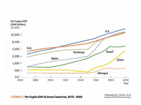
• Version of growth model we studied so far predicts thatgrowth dies out relatively quicky

• In reality, economies like U.S. have growth at ≈ 2% per yearfor more than a century

2 / 24

Adding Growth to the Growth Model

• What is missing?

• Consensus: technological progress

• Today: consequences of adding technological progress togrowth model

• Deeper and important issue: how model the process thatleads to technological progress

• probably in later lecture (“endogenous growth models”)

• what we do today will be very “reduced form”

4 / 24

Adding Growth: Choices

• Previouslyyt = F (kt , ht)

• Let At = index of technology• increase in At = technological progress

• 3 different ways to “append” At into our existing model

yt = AtF (kt , ht) neutral

yt = F (Atkt , ht) capital augmenting

yt = F (kt ,Atht) labor augmenting

• Note: if F is Cobb-Douglas, all three are isomorphic

• Result: to generate balanced growth, require thattechnological progress be labor augmenting

• Note: assumption is that tech. progress can be modeled asone-dimensional

• simplifying assumption, tech. change takes many forms

• recent work goes beyond this 5 / 24

Growth Model with Tech. Progress

• Preferences:∞∑

t=0

βtu(ct)

• Technology:

yt = F (kt ,Atht), {At}∞t=0 given

ct + it = yt

kt+1 = it + (1− δ)kt

• Endowment: k0 = k0, one unit of time each period

• Assumption: path of technological change is known

• can extend to stochastic growth model

• will likely do this in second half of semester

• Now redo everything we did before

6 / 24

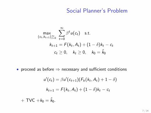
Social Planner’s Problem

max{ct ,kt+1}∞t=0

∞∑

t=0

βtu(ct) s.t.

kt+1 = F (kt ,At) + (1− δ)kt − ct

ct ≥ 0, kt ≥ 0, k0 = k0

• proceed as before ⇒ necessary and sufficient conditions

u′(ct) = βu′(ct+1)(Fk(kt ,At) + 1− δ)

kt+1 = F (kt ,At) + (1− δ)kt − ct

+ TVC +k0 = k0.

7 / 24

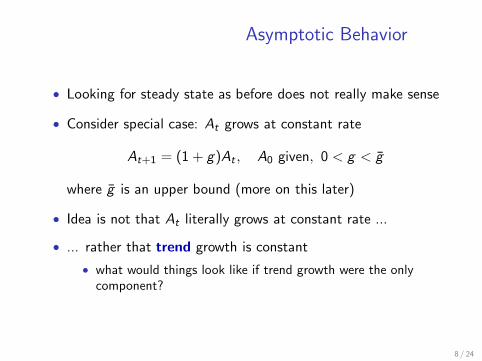
Asymptotic Behavior

• Looking for steady state as before does not really make sense

• Consider special case: At grows at constant rate

At+1 = (1 + g)At , A0 given, 0 < g < g

where g is an upper bound (more on this later)

• Idea is not that At literally grows at constant rate ...

• ... rather that trend growth is constant

• what would things look like if trend growth were the onlycomponent?

8 / 24

Balanced Growth Path

• Definition: a balanced growth path (BGP) solution to the SPproblem is a solution in which all quantities grow at constantrates

• In principle different variables could grow at different rates

• But rates turn out to be the same. To see this, consider

ct = F (kt ,At) + (1− δ)kt − kt+1

• For RHS to grow at constant rate, kt has to grow at samerate as At ⇒ ct also grows at same rate

9 / 24

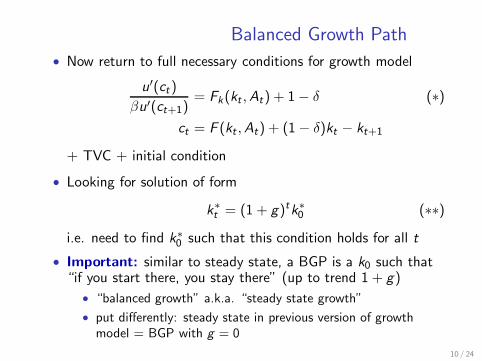
Balanced Growth Path

• Now return to full necessary conditions for growth model

u′(ct)

βu′(ct+1)= Fk(kt ,At) + 1− δ (∗)

ct = F (kt ,At) + (1− δ)kt − kt+1

+ TVC + initial condition

• Looking for solution of form

k∗t = (1 + g)tk∗0 (∗∗)

i.e. need to find k∗0 such that this condition holds for all t

• Important: similar to steady state, a BGP is a k0 such that“if you start there, you stay there” (up to trend 1 + g)

• “balanced growth” a.k.a. “steady state growth”

• put differently: steady state in previous version of growthmodel = BGP with g = 0

10 / 24

Balanced Growth Path

• Now return to full necessary conditions for growth model

u′(ct)

βu′(ct+1)= Fk(kt ,At) + 1− δ (∗)

ct = F (kt ,At) + (1− δ)kt − kt+1

+ TVC + initial condition

• If (∗∗) holds, then RHS of (∗) is constant(because CRS ⇒ Fk(kt ,At) = Fk(kt/At , 1))

• ⇒ LHS of (∗) must also be constant

• But c∗t+1 = (1+ g)c∗t . So how can we guarantee that u

′(ct )βu′(ct+1)

is constant with c∗t+1 = (1 + g)c∗t ? See next slide.

11 / 24

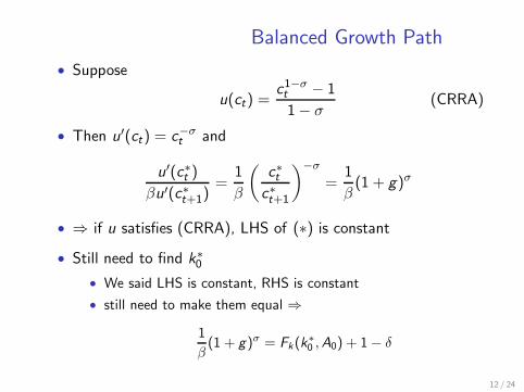
Balanced Growth Path

• Suppose

u(ct) =c1−σt − 1

1− σ(CRRA)

• Then u′(ct) = c−σt and

u′(c∗t )

βu′(c∗t+1)

=1

β

(

c∗tc∗t+1

)−σ

=1

β(1 + g)σ

• ⇒ if u satisfies (CRRA), LHS of (∗) is constant

• Still need to find k∗0

• We said LHS is constant, RHS is constant

• still need to make them equal ⇒

1

β(1 + g)σ = Fk(k

∗

0 ,A0) + 1− δ

12 / 24

Balanced Growth Path

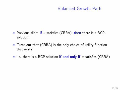
• Previous slide: if u satisfies (CRRA), then there is a BGPsolution

• Turns out that (CRRA) is the only choice of utility functionthat works

• i.e. there is a BGP solution if and only if u satisfies (CRRA)

13 / 24

Balanced Growth Path

• Only if part: note that we require

u′(c)

u′(c(1 + g))= constant for all c

• Differentiate w.r.t. c

u′′(c) = (1 + g)u′′(c(1 + g))constant

= (1 + g)u′′(c(1 + g))u′(c)

u′(c(1 + g))

u′′(c)c

u′(c)=

u′′(c(1 + g))c(1 + g)

u′(c(1 + g))

u′′(c)c

u′(c)= a (= constant)

d log u′(c)

d log c= a ⇒ log u′(c) = b + a log c

Hence u′(c) = ebca = monotone transformation of (CRRA)

14 / 24

Balanced Growth Path

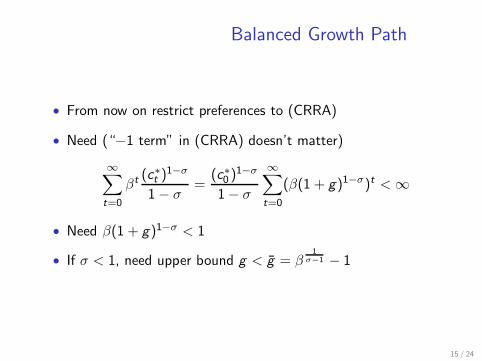
• From now on restrict preferences to (CRRA)

• Need (“−1 term” in (CRRA) doesn’t matter)

∞∑

t=0

βt(c∗t )

1−σ

1− σ=

(c∗0 )1−σ

1− σ

∞∑

t=0

(β(1 + g)1−σ)t < ∞

• Need β(1 + g)1−σ < 1

• If σ < 1, need upper bound g < g = β1

σ−1 − 1

15 / 24

Balanced Growth Path

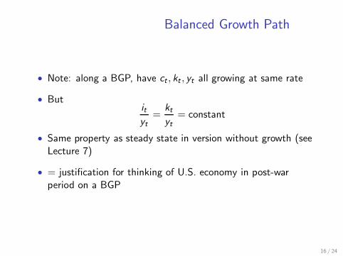
• Note: along a BGP, have ct , kt , yt all growing at same rate

• Butit

yt=

kt

yt= constant

• Same property as steady state in version without growth (seeLecture 7)

• = justification for thinking of U.S. economy in post-warperiod on a BGP

16 / 24

Transforming Model with Growth into

Model without Growth

• Know how to solve for BGP = generalization of steady state

• But what about transition dynamics? Turns out this is easy:• transform model with growth into model without growth

• analysis of transformed model same as before

• Preferences:∞∑

t=0

βtc1−σt − 1

1− σ

• Technology:

ct + kt+1 = F (kt ,At) + (1− δ)kt

• Define detrended consumption and capital

ct =ct

(1 + g)t, kt =

kt

(1 + g)t17 / 24

Transforming Model with Growth into

Model without Growth

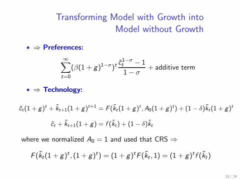
• ⇒ Preferences:

∞∑

t=0

(β(1 + g)1−σ)tc1−σt − 1

1− σ+ additive term

• ⇒ Technology:

ct(1 + g)t + kt+1(1 + g)t+1 = F (kt(1 + g)t ,A0(1 + g)t) + (1− δ)kt(1 + g)t

ct + kt+1(1 + g) = f (kt) + (1− δ)kt

where we normalized A0 = 1 and used that CRS ⇒

F (kt(1 + g)t , (1 + g)t) = (1 + g)tF (kt , 1) = (1 + g)t f (kt)

18 / 24

Transforming Model with Growth into

Model without Growth

• Hence it is sufficient to solve (drop ∼’s for simplicity)

max{ct ,kt+1}

∞∑

t=0

βtc1−σt − 1

1− σs.t.

ct + kt+1(1 + g) = f (kt) + (1− δ)kt

where β = β(1 + g)1−σ

• need β(1 + g)1−σ < 1

• same restriction as before

19 / 24

Transforming Model with Growth into

Model without Growth

• Everything else just like before. E.g. Euler equation

c−σt = βc−σ

t+1

f ′(kt+1) + 1− δ

1 + g

• Steady state

1

β=

f ′(k∗) + 1− δ

1 + g⇔

1

β(1 + g)σ = f ′(k∗) + 1− δ

• Steady state in transformed economy = BGP in originaleconomy

• transformed economy: plot log kt against t

• original economy: plot log kt against t: BGP = linear slope

log kt+1 − log kt = log

(

kt+1

kt

)

= log(1 + g) ≈ g

20 / 24

1980 1985 1990 1995 2000 2005 2010

5

10

20

40

80

Year

Per capita GDP (US=100)

United States

Japan

Western Europe

Brazil

Russia

ChinaIndia

Sub−Saharan Africa

Ten Macro Ideas – p.39/46

Prevailing Paradigmfor thinking about growth across countries

• Most countries share a long run growth rate

• for these countries, policy differences have level effects

• countries “transition around” in world BGP

• In terms of growth model

• countries i = 1, ..., n, each runs a growth model

• productivities satisfy (note: no i subscript on g)

Ait = Ai0(1 + g)teεit

• interpret Ait more broadly than technology, also includeinstitutions, policy

• every now and then, country gets εit shock, triggers transition

• Is prevailing paradigm = right paradigm?

• hard to say given data span only ≈ 100 years

• also recall from Lecture 7: transitions too fast rel. to data

23 / 24

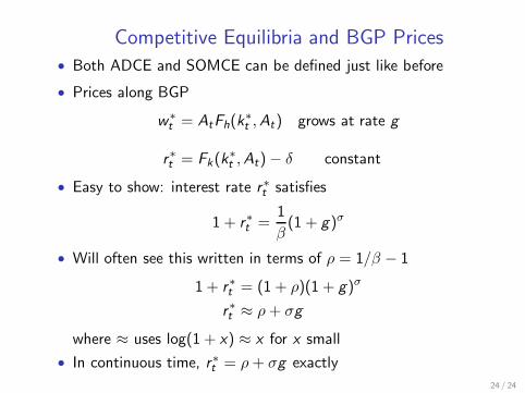
Competitive Equilibria and BGP Prices

• Both ADCE and SOMCE can be defined just like before

• Prices along BGP

w∗t = AtFh(k

∗t ,At) grows at rate g

r∗t = Fk(k∗t ,At)− δ constant

• Easy to show: interest rate r∗t satisfies

1 + r∗t =1

β(1 + g)σ

• Will often see this written in terms of ρ = 1/β − 1

1 + r∗t = (1 + ρ)(1 + g)σ

r∗t ≈ ρ+ σg

where ≈ uses log(1 + x) ≈ x for x small

• In continuous time, r∗t = ρ+ σg exactly

24 / 24