ECO 121 MACROECONOMICS

Lecture Eight

Aisha KhanSection L & M

Spring 2010

Recap

Aggregate Model

Consumption schedule Upward sloping with a slope = MPC

Saving schedule Upward sloping with a slope = MPS

Investment Demand curve Downward sloping

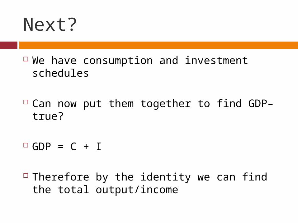
Next?

We have consumption and investment schedules

Can now put them together to find GDP– true?

GDP = C + I

Therefore by the identity we can find the total output/income

Equilibrium GDP

Employ-ment levels

GDP = DI

C S I C+I Unplanned in

inventories

Tendency of income/output

40 370 375

-5 20 395 -25

45 390 390

0 20 410 -20

50 410 405

5 20 425 -15

55 430 420

10 20 440 -10

60 450 435

15 20 455 -5

65 470 450

20 20 470 0 ~

70 490 465

25 20 485 5

75 510 480

30 20 500 10

80 530 495

35 20 515 15

85 550 510

40 20 530 20

Graphical Analysis

Aggregate expenditure C+ I

GDP

45

C

C+I

Aggregate Expenditure I = $20 billion

C+I = GDP

C = $450 billion

Other features of GDP

1. Savings = planned Investment Savings is a “leakage” from spending

stream

2. No unplanned changes in inventory Look at table again

Aggregate Expenditures

We examine now why real GDP might be unstable and subject to cyclical fluctuations

We revise the model slowly towards a more realistic model

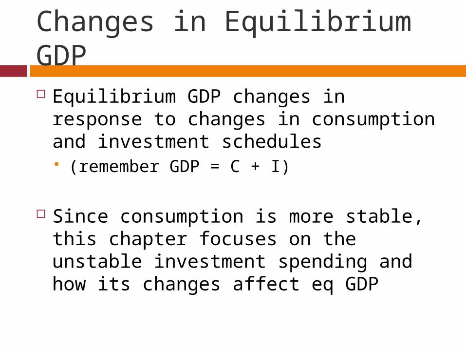
Changes in Equilibrium GDP

Equilibrium GDP changes in response to changes in consumption and investment schedules (remember GDP = C + I)

Since consumption is more stable, this chapter focuses on the unstable investment spending and how its changes affect eq GDP

Investment changes

Suppose that investment spending rises by $5 billion Due to profit expectations or changes in

the interest rate

Aggregate expenditure C+ I

GDP

45

450

C+I = GDP

(C+I)1 (C+I)0

(C+I)2

470 490

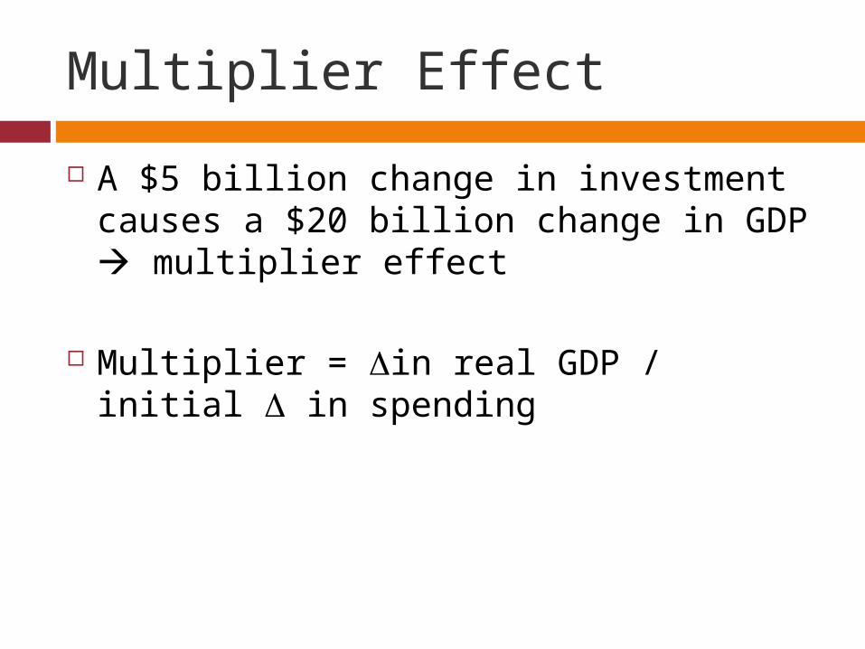
Multiplier Effect

A $5 billion change in investment causes a $20 billion change in GDP multiplier effect

Multiplier = in real GDP / initial in spending

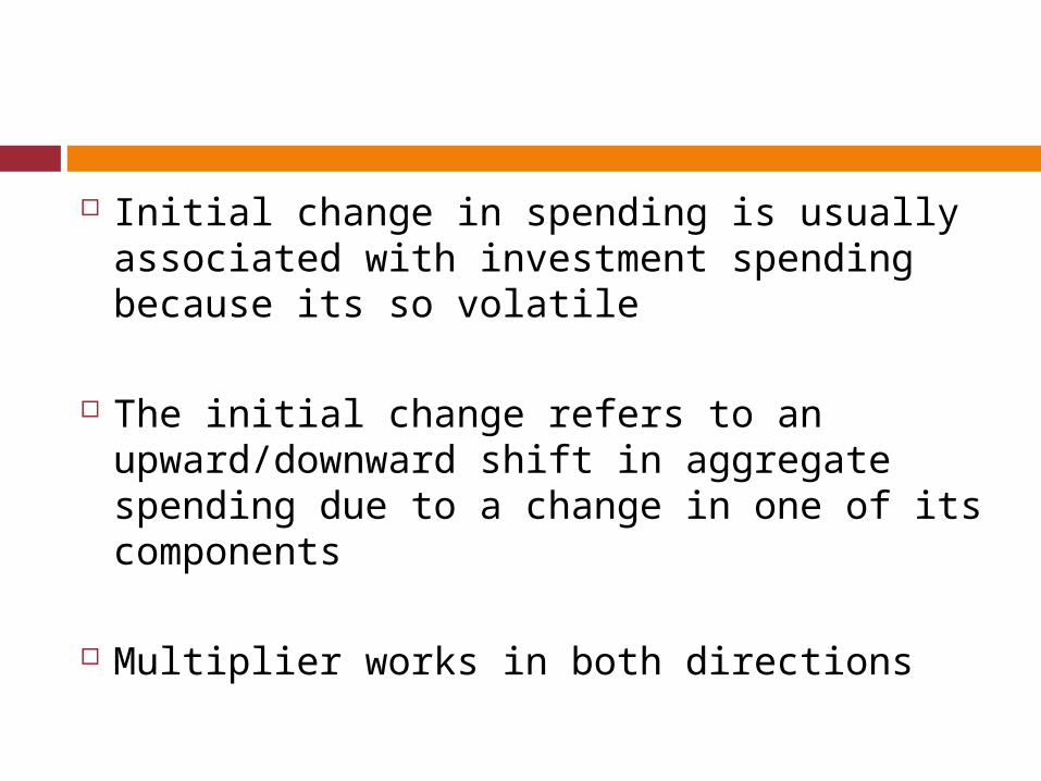
Initial change in spending is usually associated with investment spending because its so volatile

The initial change refers to an upward/downward shift in aggregate spending due to a change in one of its components

Multiplier works in both directions

Multiplier and MPC

The size of the mpc and the multiplier are directly related

The size of the mps and the multiplier are inversely related

Multiplier =1/(1-mpc) = 1/mps

International Trade and Equilibrium Output NX affect aggregate expenditures

Exports expand spending on domestic output

Imports contract spending on domestic output

Net export schedule Independent of GDP, can be positive or

negative

Positive NX ( exports > imports ) Expand spending Expansionary effect Again multiplier effect

Negative NX ( imports > exports ) Contract spending Contractionary effect

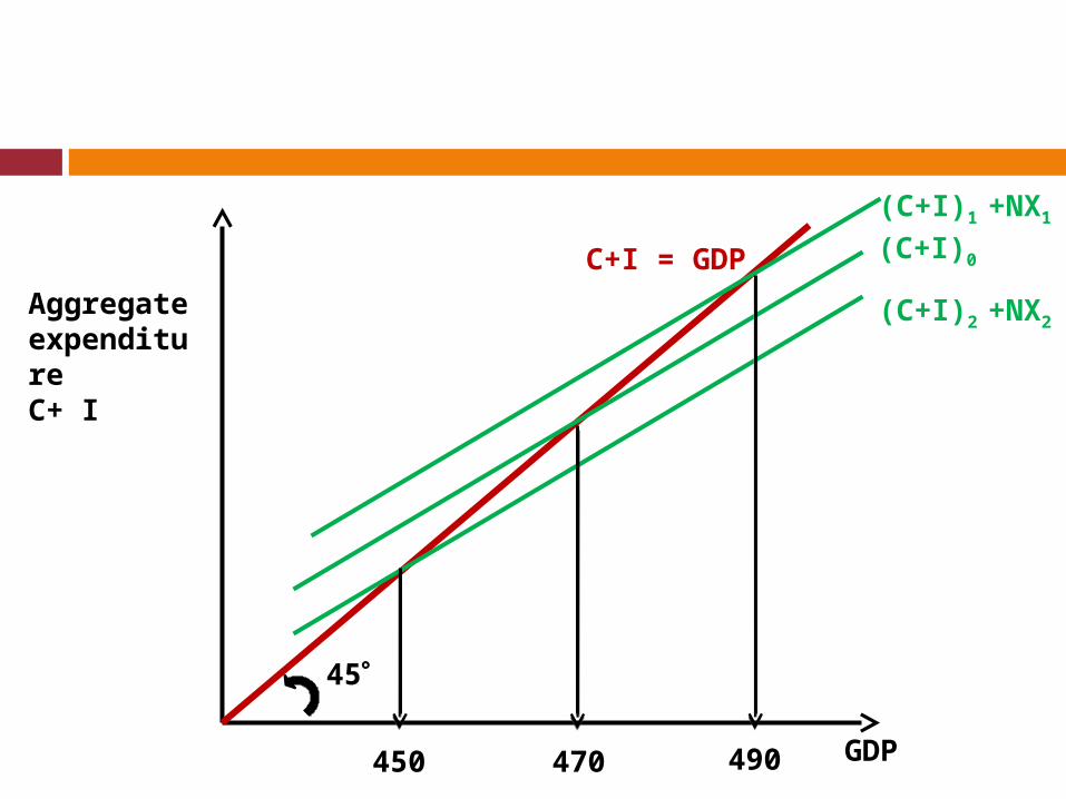
Aggregate expenditure C+ I

GDP

45

450

C+I = GDP

(C+I)1 +NX1 (C+I)0

(C+I)2 +NX2

470 490

International economic leakages Prosperity abroad generally raises our

exports

Trade barriers

Depreciation of dollar lowers cost of US goods to foreigners discouraging our exports

Adding the Public Sector

Simplifications Government purchases don’t impact

private spending Net tax revenues as personal taxes GDP = NI = PI Tax collections are independent of GDP

levels Price level is assumed to be constant

Increase in government spending boosts aggregate expenditure

Government expenditure is subject to the multiplier

Aggregate expenditure C+ I

GDP

45

C+I = GDP

(C+I)1 +NX1 + G (C+I) +NX

C

Taxes reduce DI consumption and saving lowered at each level of GDP

Therefore the sum of leakages = sum of injections

S + M + T = I + X + G