ECMWF COSPAR Training Fortaleza, Brasil, 11-Nov-2010 1 A very first introduction to data...
33
ECMWF COSPAR Training Fortaleza, Brasil, 11-Nov-2010 1 A very first introduction to data assimilation for NWP systems Joaquín Muñoz Sabater ECMWF
-
Upload
shanon-shelton -
Category
Documents
-
view
218 -
download
0
Transcript of ECMWF COSPAR Training Fortaleza, Brasil, 11-Nov-2010 1 A very first introduction to data...

ECMWF COSPAR Training Fortaleza, Brasil, 11-Nov-2010 1
A very first introduction to data assimilation for NWP systems
Joaquín Muñoz Sabater
ECMWF

ECMWF COSPAR Training Fortaleza, Brasil, 11-Nov-2010 2
► The data assimilation concept,
• Some linear estimation theory,
► Data assimilation for Numerical Weather Prediction,
► Overview of the ECMWF Data Assimilation system,
•The observations,
•The physical processes,
•The observation operator (modelled variables),
► The operational configuration at ECMWF,
► The operational schedule at ECMWF
Contents of lecture I

ECMWF COSPAR Training Fortaleza, Brasil, 11-Nov-2010 3
Why do we need data assimilation?
A crazy tool used by scientists?,
A fashion?
A magic mathematical formula which nobody understands but produces magic results?
…?

ECMWF COSPAR Training Fortaleza, Brasil, 11-Nov-2010 4
Why should we limit our speed?

ECMWF COSPAR Training Fortaleza, Brasil, 11-Nov-2010 5
How to ‘control’ our speed? Observables

ECMWF COSPAR Training Fortaleza, Brasil, 11-Nov-2010 6
Radar Speedometer
yr = 110 km/h ys = 95 km/h
What is the best estimation of the speed x of the vehicle?
Control variable : x speed of the car,
« Truth » : xt real speed of the car (unknown),
Observation 1 : yr speed given by radar,
Observation 2 : ys speed given by speedometer
Problem description; linear estimation

ECMWF COSPAR Training Fortaleza, Brasil, 11-Nov-2010 7
Radar Speedometer
yr = 110 km/h ys = 95 km/h
Problem description; linear estimation

ECMWF COSPAR Training Fortaleza, Brasil, 11-Nov-2010 8
Radar Speedometer
yr = 110 km/h ys = 95 km/h
Case 1) Police officer believe the radar measurement
Problem description; linear estimation

ECMWF COSPAR Training Fortaleza, Brasil, 11-Nov-2010 9
Radar Speedometer
yr = 110 km/h ys = 95 km/h
Case 1) Police officer believe the radar measurement
x = yr = 110 Km/h the driver will pay a traffic fine
Problem description; linear estimation
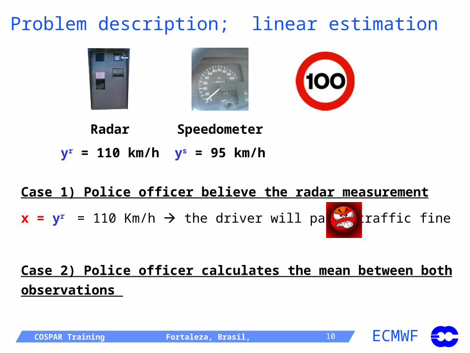
ECMWF COSPAR Training Fortaleza, Brasil, 11-Nov-2010 10
Radar Speedometer
yr = 110 km/h ys = 95 km/h
Case 1) Police officer believe the radar measurement
x = yr = 110 Km/h the driver will pay a traffic fine
Case 2) Police officer calculates the mean between both observations
Problem description; linear estimation

ECMWF COSPAR Training Fortaleza, Brasil, 11-Nov-2010 11
Radar Speedometer
yr = 110 km/h ys = 95 km/h
Case 1) Police officer believe the radar measurement
x = yr = 110 Km/h the driver will pay a traffic fine
Case 2) Police officer calculates the mean between both observations
x = yr/2 + ys/2 = 102.5 km/h the driver will pay a traffic fine
Problem description; linear estimation

ECMWF COSPAR Training Fortaleza, Brasil, 11-Nov-2010 12
Radar Speedometer
yr = 110 km/h ys = 95 km/h
Case 3) Best Linear Unbiased Estimator with all the information,
x = C1 yr + C2 ys
Hypothesis (BLUE): 1) E[] = 0,
2) σ2x min
r = 10 km/h s = 5 km/h
Problem description; linear estimation
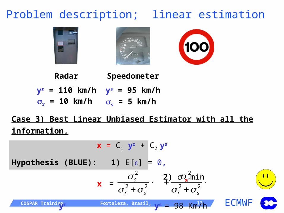
ECMWF COSPAR Training Fortaleza, Brasil, 11-Nov-2010 13
Radar Speedometer
yr = 110 km/h ys = 95 km/h
Case 3) Best Linear Unbiased Estimator with all the information,
x = C1 yr + C2 ys
Hypothesis (BLUE): 1) E[] = 0,
2) σ2x min
yr ys = 98 Km/h
r = 10 km/h s = 5 km/h
x =
22
2
22
2
sr
r
sr
s
Problem description; linear estimation

ECMWF COSPAR Training Fortaleza, Brasil, 11-Nov-2010 14
Radar Speedometer
yr = 110 km/h ys = 95 km/hr = 10 km/h s = 5 km/h
Generalization with p observations
Chronometer
ym = 85 km/h
m = 4 km /h
[p] observations
…
xa = (HTR-1H)-1 HTR-1 y
xa Control vector (analysed variables); [va, da, aa,…]
y vector of observations; [yr, ys, ym,…]
R variance-covariance matrix of observations; Rii = i2 ; Rij = ij
H non-linear observation operator; y = H (x)
xa = K y
y = H (xt) + ε

ECMWF COSPAR Training Fortaleza, Brasil, 11-Nov-2010 15
Generalization with first-guess
xa = xb + HBT(HBHT+R)-1 (y-Hxb)
xa Control vector (analysed)
xb first-guess vector (in NWP forecast by meteorological model)
y vector of observations
H non-linear observation operator yo = H(xt)+
HBT(HBHT+R)-1 Gain K
B variance-covariance matrix of first-guess
R variance-covariance matrix of observations
Radar Speedometer
yr = 110 km/h ys = 95 km/h
r = 10 km/h s = 5 km/h
Chronometerym = 85 km/h
m = 4 km /h
[p]
observations
…
Physical model
xb

ECMWF COSPAR Training Fortaleza, Brasil, 11-Nov-2010 16
But why data assimilation in NWP?
1. Improve model initial conditions for better model forecasts,
2. Better representation of
Observation errors (and their probabilistic distribution),
Model errors (and their probability distributions),
Correlations between Observations/Model,
3. Analysis of the role of different DA methodologies to improve weather forecast (minimizations, approximations, etc.),
4. Understanding of the interaction between different physical processes,
5. Others (cal/val, scalability in NWP, etc.)

ECMWF COSPAR Training Fortaleza, Brasil, 11-Nov-2010 17
Data assimilation for weather prediction
Non-analysed fc
temps
Mo
del
led
var
iab
les
(Tem
per
atu
re, h
um
itid
y,et
c)
12h-forecast
observations
observations
00 UTC 12 UTC
12h-forecast
Analysis
00 UTC (+ 24h)
Sequential methods

ECMWF COSPAR Training Fortaleza, Brasil, 11-Nov-2010 18
Data assimilation for weather prediction
Non-analysed fc
temps
Mo
del
led
var
iab
les
(Tem
per
atu
re, h
um
itid
y,et
c)
12h-forecast
observations
observations
00 UTC 12 UTC
12h-forecast
Analysis
00 UTC (+ 24h)
But…
Observations are irregularly distributed in time and space,
Matrices R and B contain millions of observations, inverting (HBHT+R) is very expensive.
Linear assumptions have to be done.
Sequential methods

ECMWF COSPAR Training Fortaleza, Brasil, 11-Nov-2010 19
Data assimilation for weather prediction
time
Co
ntr
ol v
aria
ble
Minimisation of a cost function:
observationssimulations
JoJo
Jo
Jo
Jb
Assimilation window (12h)
)(2
)(2
)(11
xHyR
xHyxxB
xxxJ TbTb
JoJb
First-guess trajetory
Corrected trajectory
Variational methods
ECMWF COSPAR Training Fortaleza, Brasil, 11-Nov-2010 20
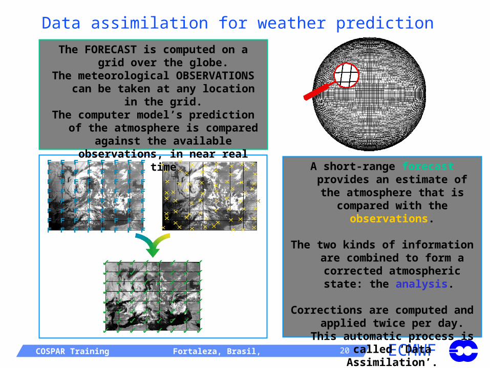
Data assimilation for weather prediction
A short-range forecast provides an estimate of the atmosphere that
is compared with the observations.
The two kinds of information are combined to form a corrected
atmospheric state: the analysis.
Corrections are computed and applied twice per day. This automatic process is called
‘Data Assimilation’.
The FORECAST is computed on a grid over the globe.
The meteorological OBSERVATIONS can be taken at any location in the grid.
The computer model’s prediction of the atmosphere is compared against the available observations, in near real
time
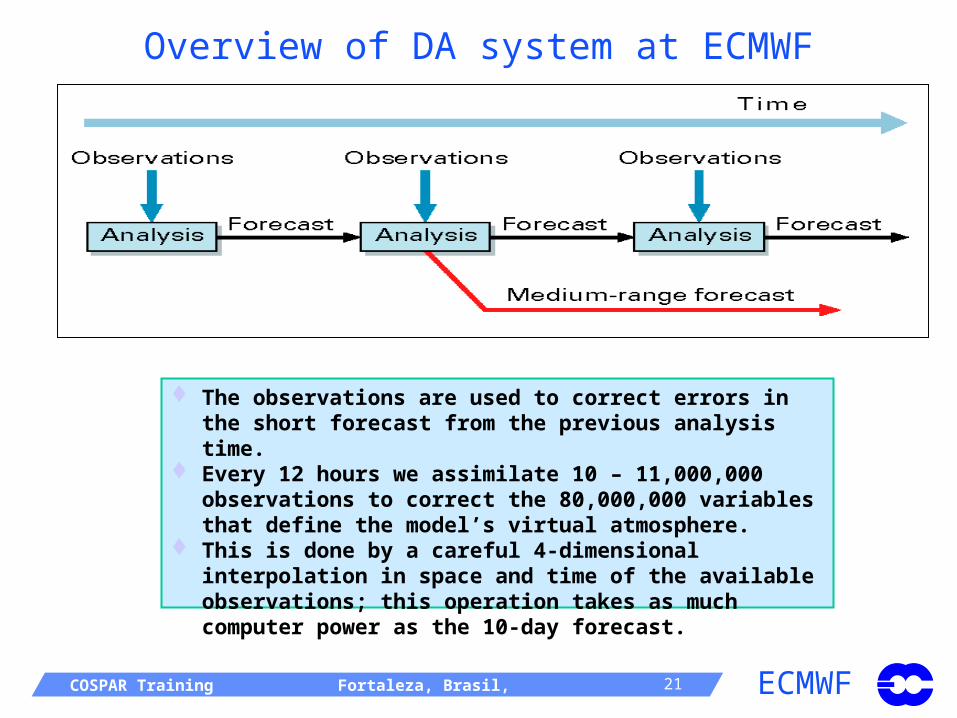
ECMWF COSPAR Training Fortaleza, Brasil, 11-Nov-2010 21
Overview of DA system at ECMWF
The observations are used to correct errors in the short forecast from the previous analysis time.
Every 12 hours we assimilate 10 – 11,000,000 observations to correct the 80,000,000 variables that define the model’s virtual atmosphere.
This is done by a careful 4-dimensional interpolation in space and time of the available observations; this operation takes as much computer power as the 10-day forecast.

ECMWF COSPAR Training Fortaleza, Brasil, 11-Nov-2010 22
Conventional observations used
MSL Pressure, 10m-wind, 2m-Rel.Hum. DRIBU: MSL Pressure, Wind-10m
Wind, Temperature, Spec. Humidity PILOT/Profilers: Wind
Aircraft: Wind, Temperature
SYNOP/METAR/SHIP:
Radiosonde balloons (TEMP):
Note: We only use a limited number of the observed variables; especially over land.

ECMWF COSPAR Training Fortaleza, Brasil, 11-Nov-2010 23
Satellite data very important
Satellite measurements are increasingly important: Global coverage (often only source of observations over ocean and remote land)
High spatial and temporal resolution
Decrease in conventional observing networks (fewer radiosonde stations)
But satellite data are not easy to use: Satellites do not measure the model variables (temperature, wind, humidity)
They measure radiances, so
either use derived products (e.g. cloud motion and scatterometer winds)
or calculate ‘model radiances’ and compare with observations
Recent developments in data assimilation are designed to improve the use of satellite data
Variational data assimilation: can use radiance data directly
Added model levels in upper stratosphere allows use of additional satellite data
4D-Var: use observations at appropriate time
Increased resolution – more in agreement with the resolution of measurements

ECMWF COSPAR Training Fortaleza, Brasil, 11-Nov-2010 24
Satellite data sources used in the operational ECMWF analysis
Geostationary, 4 IR and 5 winds
5 imagers: 3xSSM/I, AMSR-E, TMI
4 ozone
13 Sounders: NOAA AMSU-A/B, HIRS, AIRS, IASI, MHS
2 Polar, winds: MODIS
3 Scatterometer sea winds: ERS, ASCAT, QuikSCAT
6 GPS radio occultation

ECMWF COSPAR Training Fortaleza, Brasil, 11-Nov-2010 25
Significant increase in number of observations assimilated
Conventional and satellite data assimilated at ECMWF 1996-2010
ECMWF COSPAR Training Fortaleza, Brasil, 11-Nov-2010 26
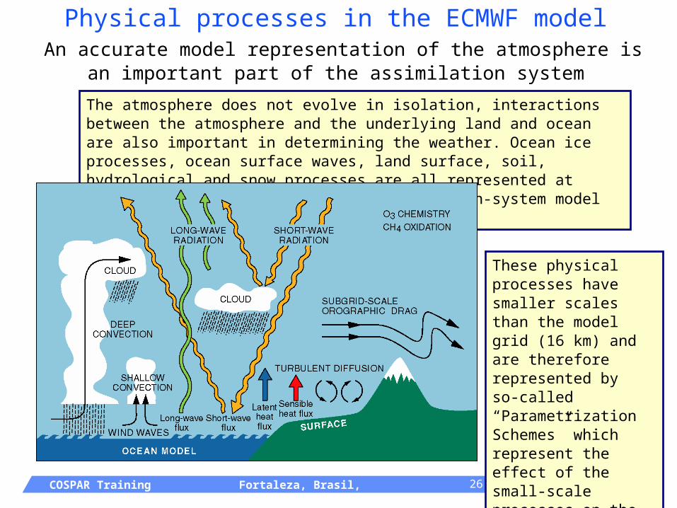
The atmosphere does not evolve in isolation, interactions between the atmosphere and the underlying land and ocean are also important in determining the weather. Ocean ice processes, ocean surface waves, land surface, soil, hydrological and snow processes are all represented at ECMWF in the most advanced operational Earth-system model available anywhere.
These physical processes have smaller scales than the model grid (16 km) and are therefore represented by so-called “Parametrization Schemes” which represent the effect of the small-scale processes on the large-scale flow.
Physical processes in the ECMWF model An accurate model representation of the atmosphere is an
important part of the assimilation system
ECMWF COSPAR Training Fortaleza, Brasil, 11-Nov-2010 27
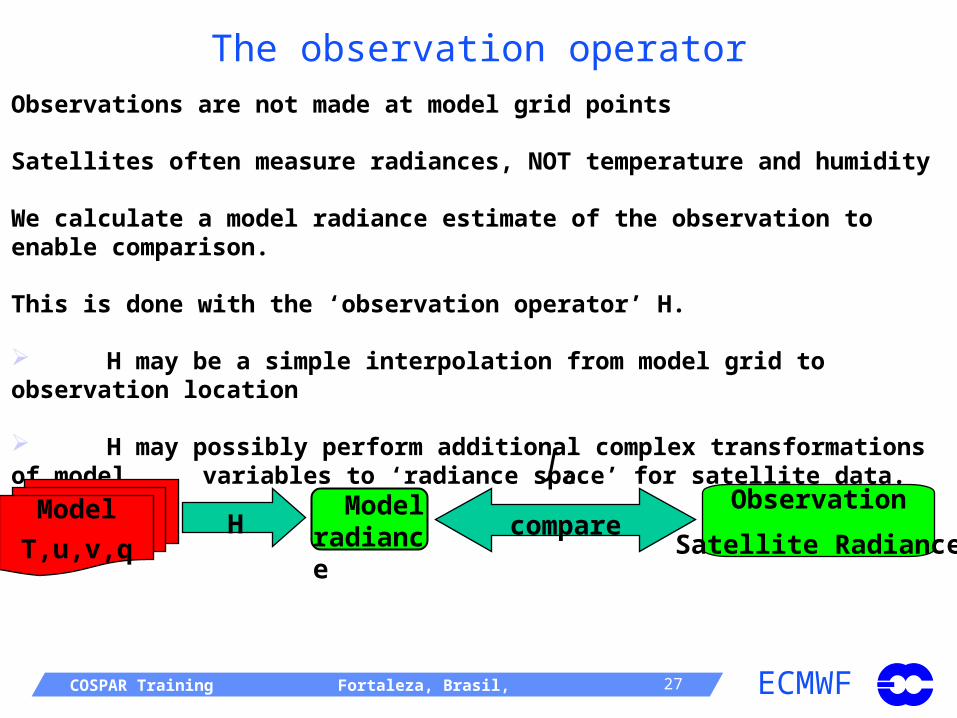
The observation operatorObservations are not made at model grid points
Satellites often measure radiances, NOT temperature and humidity
We calculate a model radiance estimate of the observation to enable comparison.
This is done with the ‘observation operator’ H.
H may be a simple interpolation from model grid to observation location
H may possibly perform additional complex transformations of model variables to ‘radiance space’ for satellite data.
Model
T,u,v,q
Observation
Satellite Radiancecompare
oJ
H Model radiance
ECMWF COSPAR Training Fortaleza, Brasil, 11-Nov-2010 28
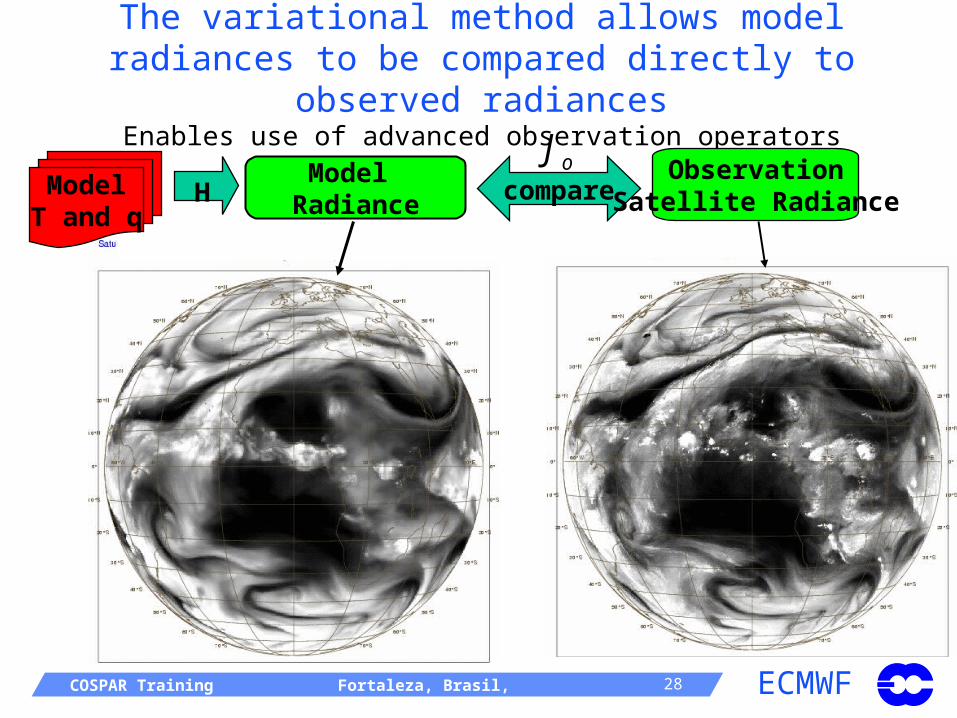
Model Radiance
The variational method allows model radiances to be compared directly to observed radiances
Enables use of advanced observation operators
ModelT and q
H compareObservation
Satellite Radiance
oJ
ECMWF COSPAR Training Fortaleza, Brasil, 11-Nov-2010 29
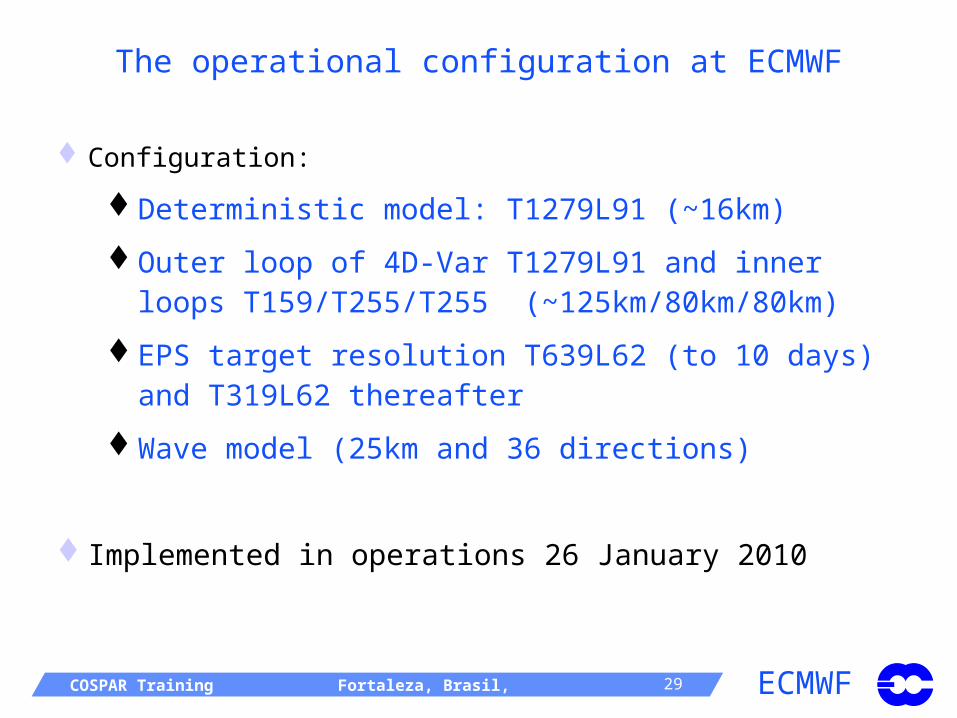
The operational configuration at ECMWF
Configuration:
Deterministic model: T1279L91 (~16km)
Outer loop of 4D-Var T1279L91 and inner loops T159/T255/T255 (~125km/80km/80km)
EPS target resolution T639L62 (to 10 days) and T319L62 thereafter
Wave model (25km and 36 directions)
Implemented in operations 26 January 2010

ECMWF COSPAR Training Fortaleza, Brasil, 11-Nov-2010 30
Extract data for 12h period 2100-0900UTC
70sec (min. 8x1PEs)
Pre-process satellite data. Cloud clearing. Scatterometer winds.
340sec (min. 16x1PEs)
Observation pre-processing for 0000UTC main cycle

ECMWF COSPAR Training Fortaleza, Brasil, 11-Nov-2010 31
Analysis and forecast for 0000UTC main cycle BUFR to ODB.
200sec 4x(8-16PEs)
Fetch background forecast 275sec 2x(1PE)
Analysis: trajectory, minimization and update 4320sec (3072PEs)
10 day forecast. 1440 t-steps
3070sec (3072PEs)
(or 15h fc for cycling: 260sec)
Surface analysis.
1010sec 4x(1PEs)
430s
260s880s
270s 820s
490s
1110s
ECMWF COSPAR Training Fortaleza, Brasil, 11-Nov-2010 32
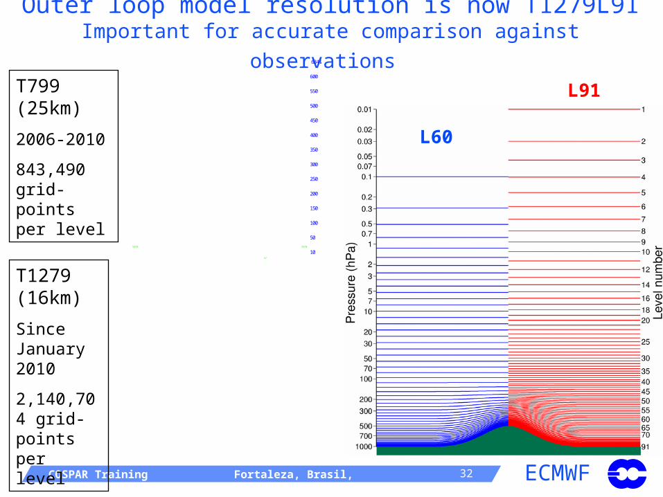
T1279 (16km)
Since January 2010
2,140,704 grid-points per level
Outer loop model resolution is now T1279L91 Important for accurate comparison against observations
L60
L91T799 (25km)
2006-2010
843,490 grid-points per level
50°N 50°N
0°
0°
Orography at T799
10
50
100
150
200
250
300
350
400
450
500
550
600
634.0
50°N 50°N
0°
0°
Orography at T1279
10
50
100
150
200
250
300
350
400
450
500
550
600
650
684.1

ECMWF COSPAR Training Fortaleza, Brasil, 11-Nov-2010 33
Operational schedule Early delivery suite introduced June 2004
3hFC
6h 4D-Var
21-03Z
00 UTC analysis (DA)
T1279 10 day forecast
51*T639/T399 EPS forecasts
03:40
04:00
04:40
06:05
05:00
Disseminate
06:35
Disseminate Disseminate
02:00
12h 4D-Var, obs 09-21Z
18 UTC analysis
03:30
3hFC
6h 4D-Var
9-15Z
12 UTC analysis (DA)
T1279 10 day forecast
51*T639/T399 EPS forec.
15:40
16:00
16:40
18:05
17:00
Disseminate Disseminate
14:00
12h 4D-Var, obs 21-09Z
06 UTC analysis
15:30