Echo State Networks for Self-Organizing Resource Allocation in … · · 2016-01-27Echo State...
29
Echo State Networks for Self-Organizing Resource Allocation in LTE-U with Uplink-Downlink Decoupling Mingzhe Chen * , Walid Saad † , and Changchuan Yin * * Beijing Key Laboratory of Network System Architecture and Convergence, Beijing University of Posts and Telecommunications, Beijing, China 100876 Email: [email protected] and [email protected]. † Wireless@VT, Bradley Department of Electrical and Computer Engineering, Virginia Tech, Blacksburg, VA, USA, Email: [email protected] Abstract Uplink-downlink decoupling in which users can be associated to different base stations in the uplink and downlink of heterogeneous small cell networks (SCNs) has attracted significant attention recently. However, most existing works focus on simple association mechanisms in LTE SCNs that operate only in the licensed band. In contrast, in this paper, the problem of resource allocation with uplink-downlink decoupling is studied for an SCN that incorporates LTE in the unlicensed band (LTE- U). Here, the users can access both licensed and unlicensed bands while being associated to different base stations. This problem is formulated as a noncooperative game that incorporates user association, spectrum allocation, and load balancing. To solve this problem, a distributed algorithm based on the machine learning framework of echo state networks is proposed using which the small base stations autonomously choose their optimal bands allocation strategies while having only limited information on the network’s and users’ states. It is shown that the proposed algorithm converges to a stationary mixed-strategy distribution which constitutes a mixed strategy Nash equilibrium for the studied game. Simulation results show that the proposed approach yields significant gains, in terms of the sum-rate of the 50th percentile of users, that reach up to 60% and 78%, respectively, compared to Q-learning and Q-learning without decoupling. The results also show that ESN significantly provides a considerable reduction of information exchange for the wireless network. Index Terms— game theory; resource allocation; heterogeneous networks; reinforcement learning; LTE-U. arXiv:1601.06895v1 [cs.IT] 26 Jan 2016
Transcript of Echo State Networks for Self-Organizing Resource Allocation in … · · 2016-01-27Echo State...
Echo State Networks for Self-Organizing Resource
Allocation in LTE-U with Uplink-Downlink Decoupling
Mingzhe Chen∗, Walid Saad†, and Changchuan Yin∗∗Beijing Key Laboratory of Network System Architecture and Convergence,
Beijing University of Posts and Telecommunications, Beijing, China 100876
Email: [email protected] and [email protected].†Wireless@VT, Bradley Department of Electrical and Computer Engineering, Virginia Tech, Blacksburg, VA,
USA, Email: [email protected]
Abstract
Uplink-downlink decoupling in which users can be associated to different base stations in the
uplink and downlink of heterogeneous small cell networks (SCNs) has attracted significant attention
recently. However, most existing works focus on simple association mechanisms in LTE SCNs that
operate only in the licensed band. In contrast, in this paper, the problem of resource allocation with
uplink-downlink decoupling is studied for an SCN that incorporates LTE in the unlicensed band (LTE-
U). Here, the users can access both licensed and unlicensed bands while being associated to different
base stations. This problem is formulated as a noncooperative game that incorporates user association,
spectrum allocation, and load balancing. To solve this problem, a distributed algorithm based on the
machine learning framework of echo state networks is proposed using which the small base stations
autonomously choose their optimal bands allocation strategies while having only limited information
on the network’s and users’ states. It is shown that the proposed algorithm converges to a stationary
mixed-strategy distribution which constitutes a mixed strategy Nash equilibrium for the studied game.
Simulation results show that the proposed approach yields significant gains, in terms of the sum-rate of
the 50th percentile of users, that reach up to 60% and 78%, respectively, compared to Q-learning and
Q-learning without decoupling. The results also show that ESN significantly provides a considerable
reduction of information exchange for the wireless network.
Index Terms— game theory; resource allocation; heterogeneous networks; reinforcement learning; LTE-U.
arX
iv:1
601.
0689
5v1
[cs
.IT
] 2
6 Ja
n 20
16
2
I. INTRODUCTION
The recent surge in wireless services has led to significant changes in existing cellular systems
[1]. In particular, the next-generation of cellular systems will be based on small cell networks
(SCNs) that rely on low-cost, low-power small base stations (SBSs). The ultra dense nature of
SCNs coupled with the transmit power disparity between SBSs, further motivates the use of
uplink-downlink decoupling techniques [2], [3] in which users can associate to different SBSs
in the uplink and downlink, respectively. Such techniques have become recently very popular,
particularly with the emergence of uplink-intensive applications such as machine-to-machine
communications or even social networks.
Existing literature has studied a number of problems related to uplink-downlink decoupling
[2], [3]. In [2], the authors delineate the main benefits of decoupling the uplink and downlink,
and propose an optimal decoupling association strategy that maximizes data rate. The work
in [3] investigates the throughput and outage gains of uplink-downlink decoupling using a
simulation approach. Despite the promising results, these existing works [2], [3] are restricted
to performance analysis and centralized optimization approaches that may not scale well in a
dense and heterogeneous SCN. Moreover, these existing works are restricted to classical LTE
networks in which the devices and SBSs can access only a single, licensed band.
Recently, there has been significant interest in studying how LTE-based SCNs can operate in
the unlicensed band (LTE-U) [4]–[11]. LTE-U presents many challenges in terms of spectrum
allocation, user association, and interference management [4]–[6]. In [4], optimal resource allo-
cation algorithms are proposed for both dual band femtocell and integrated femto-WiFi networks.
The authors in [5] develop a hybrid method to perform both traffic offloading and resource sharing
in an LTE-U scenario with a single base station (BS). In [6], a novel performance analysis that
accounts for system-level dynamics is performed and an enabling architecture that captures the
tight interaction between different radio access technologies is proposed. However, most existing
works on LTE-U [4]–[11] have focused on the performance analysis and resource allocation with
conventional association methods. Indeed, none of these works analyzed the potential of uplink-
downlink decoupling in LTE-U. LTE-U provides an ideal setting to perform uplink-downlink
decoupling, since beyond the spatial dimension, the possibility of uplink-downlink decoupling
exists not only between base stations but also between the licensed and unlicensed bands.
3
More recently, reinforcement learning (RL) has gained significant attention for developing
distributed approaches for resource allocation in LTE and heterogeneous SCNs [12]–[20]. In
[13]–[16] and [20], channel selection, network selection, and interference management were
addressed using the framework of Q-learning and smoothed best response. In [17]–[19], regret-
based learning approaches are developed to address the problem of interference management,
dynamic clustering, and SBSs’ on/off. However, none of the existing works on RL [12]–[20]
have focused on the LTE-U network and downlink-uplink decoupling. Moreover, most existing
algorithms [12]–[20], require agents to obtain the other agents’ value functions [21] and state
information, which is not practical for scenarios in which agents are distributed. In contrast,
here, our goal is to develop a novel and efficient multi-agent RL algorithm based on recurrent
neural networks (RNNs) [22]–[27] whose advantage is that they can store the state informations
of users and have no need to share value functions between agents.
Since RNNs have the ability to retain state over time, because of their recurrent connections,
they are promising candidates for compactly storing moments of series of observations. Echo
state networks, an emerging RNN framework [22]–[27], are a promising candidate for wireless
network modeling, as they are known to be relatively easy to train. Existing literature has studied a
number of problems related to ESNs [22]–[25]. In [22]–[24], ESNs are proposed to model reward
function, characterize wireless channels, and equalize the non-linear satellite communication
channel. The authors in [25], prove the convergence of ESNs-RL algorithm under the condition
of Markov decision problems and exploits ESNs-RL algorithm to settle the maze and tiger
problems. However, most existing works on ESNs [22]–[25] have just focused on the problems
of traditional RNNs and wireless channel. In addition, none of these works exploited the use of
ESNs for resource allocation problem in a wireless network.
The main contribution of this paper is to develop a novel, self-organizing framework to
optimize resource allocation with uplink-downlink decoupling in an LTE-U system. We formulate
the problem as a noncooperative game in which the players are the SBSs and the macrocell base
station (MBS). Each player seeks to find an optimal spectrum allocation scheme to optimize a
utility function that captures the sum-rate in terms of downlink and uplink, and balances the
licensed and unlicensed spectrums between users. To solve this resource allocation game, we
propose a self-organizing algorithm based on the powerful framework of ESNs [25]–[27]. Unlike
previous studies [4], [5], which rely on the coordination among SBSs and on the knowledge
4
of the entire users’ state informations, the proposed approach requires minimum information
to learn the mixed strategy Nash equilibrium. The use of ESNs enables the LTE-U SCN to
quickly learn its resource allocation parameters without requiring significant training data. The
proposed algorithm enables dual-mode SBSs to autonomously learn and decide on the allocation
of the licensed and unlicensed bands in the uplink and downlink to each user depending on the
network environment. Moreover, we show that the proposed ESN algorithm can converge to a
mixed strategy Nash equilibrium. To our best knowledge, this is the first work that exploits the
framework of ESNs to optimize resource allocation with uplink-downlink decoupling in LTE-U
systems. Simulation results show that the proposed approach yields a performance improvement,
in terms of the sum-rate of the 50th percentile of users, reaching up to 60% and 78%, respectively,
compared to Q-learning and Q-learning without decoupling.
The rest of this paper is organized as follows. The system model is described in Section II.
The ESN-based resource allocation algorithm is proposed in Section III. In Section IV, numerical
simulation results are presented and analyzed. Finally, conclusions are drawn in Section V.
II. SYSTEM MODEL AND PROBLEM FORMULATION
Consider the downlink and uplink of an SCN that encompasses LTE-U, WiFi access points,
and a macrocell network. Here, the macrocell tier operates using only the licensed band. The
MBS is located at the center of a geographical area. Within this area, we consider a set N =
{1, 2, . . . , Ns} of dual-mode SBSs that are able to access both the licensed and unlicensed bands.
Co-located with this cellular network is a WiFi network that consists of W WiFi access points. In
addition, we consider a set U = {1, 2, · · · , U} of U LTE-U users which are distributed uniformly
over the area of interest. All users can access different SBSs as well as the MBS for transmitting
in the downlink or uplink. For this system, we consider a frequency division duplexing (FDD)
mode for LTE on the licensed band, which splits the licensed band into equal spectrum bands
for the downlink and uplink. Time division duplexing (TDD) mode LTE with listen before talk
mechanism is considered on the unlicensed band [11]. Here, the unlicensed band is used for both
the downlink and uplink, just like in a conventional LTE TDD system. For LTE-U operating
in the unlicensed band, TDD offers the flexibility to adjust the resource allocation between the
downlink and uplink. The WiFi access points will transmit using a standard carrier sense multiple
access with collision avoidance (CSMA/CA) protocol with its corresponding RTS/CTS access

5
mechanism.
A. LTE data rate analysis
We denote by Bl the set of the MBS and SBSs on the licensed band. During the connection
period, we denote by cDLlij the downlink capacity and cUL
lji the uplink capacity on the licensed
band. Thus, the overall long-term downlink and uplink rates of the LTE-U user i on the licensed
band are given by:
RDLlij = dijc
DLlij , (1)
RULlji = vjic
ULlji , (2)
where
cDLlij =F
DLl log2
1+ Pjhij∑k∈Bl,k 6=j
Pkhik+σ2
,
cULlji =F
ULl log2
1+ Puhij∑k∈U ,k 6=i
Puhkj+σ2
,dij and vji are the fraction of the downlink and uplink licensed bands allocated from SBS j to
user i, respectively, FDLl and FUL
l denote, respectively, the downlink and uplink bandwidths on
the licensed band, Pj is the transmit power of the BS j, Pu is the transmit power of LTE-U
users, hij is the channel gain between user i and BS j, and σ2 is the power of the Gaussian
noise. Note that, hereinafter, we use the term BS to refer to either an SBS or the MBS and
denote by B the set of BSs.
Similarly, the downlink and uplink rates of user i that is transmitting over the unlicensed band
are given by:
RDLuij = κijc
DLuij, (3)
RULuji = τjic
ULuji, (4)
where
cDLuij = LFulog2
1 +Pjhij∑
k∈Bu,k 6=jPwhik + σ2
,
6
cULuji=LFulog2
1+ Puhij∑k∈U ,k 6=i
Puhkj+σ2
,L denotes the SBSs occupy time slots of the unlicensed band, κij and τji denote, respectively,
the downlink and uplink time slots during which user i transmits on the unlicensed band. Note
that, the SBSs adopt a TDD mode on the unlicensed band and the LTE-U users on the uplink
and downlink share the time slots of the unlicensed band. Fu denotes the bandwidth of the
unlicensed band, Bu denotes the SBSs on the unlicensed band, and L ∈ [0, 1] is the time slots
during which the LTE SCN uses the unlicensed band.
B. WiFi data rate analysis
For the WiFi network, we assume that the WiFi access points will adopt a CSMA/CA scheme
with binary slotted exponential backoff. Therefore, the saturation capacity of Nw users sharing
the same unlicensed band can be expressed by [28]:
R (Nw) =PtrPsE [P ]
(1− Ptr)Tσ + PtrPsTs + Ptr (1− Ps)Tc, (5)
where Ptr = 1 − (1− ς)Nw , Ptr is the probability that there is at least one transmission in a
time slot and ς is the transmission probability of each user. Ps = Nwς(1− ς)Nw−1/Ptr , is the
successful transmission on the channel, Ts is the average time that the channel is sensed busy
because of a successful transmission, Tc is the average time that the channel is sensed busy by
each station during a collision, Tσ is the duration of an empty slot time, and E [P ] is the average
packet size.
In our model, the WiFi network adopts conventional distributed coordination function (DCF)
access and RTS/CTS access mechanisms. Thus, Tc and Ts are given by [28]:
Ts =RTS/C + CTS/C + (H + E [P ])/C
+ ACK/C + 3SIFS +DIFS + 4δ,(6)
Tc = RTS/C +DIFS + δ, (7)
where Ts denotes the average time the channel is sensed busy because of a successful trans-
mission, Tc is the average time the channel is sensed busy by each station during a collision,

7
H = PHYhdr +MAChdr, C is the channel bit rate, and ACK, DIFS, δ, RTS, and CTS are
WiFi parameters.
In our model, the SBSs occupy L time slots on the unlicensed band. Thus, the WiFi users
occupy the (1− L) time slots and the per WiFi user rate is:
Rw =R (Nw) (1− L)
Nw
, (8)
where Nw is the number of WiFi users on the unlicensed band.
C. Problem formulation
Given this system model, our goal is to develop an effective spectrum allocation scheme with
uplink-downlink decoupling that can allocate the appropriate bandwidth on the licensed band and
time slots on the unlicensed band to each user, simultaneously. However, the rate of each SBS
depends not only on its own choice of the allocation action but also on remaining SBSs’ actions.
In this regard, we formulate a noncooperative game G =[B, {An}n∈B , {un}n∈B
]in which the
set of BSs B are the players including SBSs and the MBS and un is the utility function for BS
n. Each player n has a set An ={an,1, . . . ,an,|An|
}of actions where |An| is the total number of
actions. For an SBS n, each action an = (dn,vn,ρn), is composed of: (i) the downlink licensed
bandwidth allocation dn = [dn,1, . . . , dn,Kn ], where Kn is the number of all users in the coverage
area Lb of SBS n, (ii) the uplink licensed bandwidth allocation vn = [vn,1, . . . vn,Kn ], and, (iii)
the time slots allocation on the unlicensed band ρn = [κ1,n, . . . , κKn,n, τn,1, . . . , τn,Kn ]. dn, vn
and ρn must satisfy: ∑Kn
j=1dn,j ≤ 1,
∑Kn
j=1vn,j ≤ 1, (9)∑Kn
j=1(κn,j + τj,n) ≤ 1, (10)
djn, vnj, κnj, τjn ∈ Z. (11)
where Z = {1, . . . , Z} is a finite set of Z level fractions of spectrum. For example, one
can separate the fractions of spectrum into Z = 10 equally spaced intervals. Then, we will
have Z = {0, 0.1, . . . , 0.9, 1}. For the MBS, each action am = (dm,vm) is composed of
its downlink licensed bandwidth allocation dm and uplink licensed bandwidth allocation vm.
a = (a1,a2, . . . ,aNb) ∈ A, represents the action profile of all players where Nb = Ns + 1,
expresses the number of BSs including one MBS and Ns SBSs, and A =∏
n∈Nb An.
8
To maximize the downlink and uplink rates simultaneously while maintaining load balancing,
for each SBS n, the utility function needs to capture both the sum data rate and load balancing.
Here, load balancing implies that each BS will balance its spectrum allocation between users,
while taking into account their capacity. Therefore, we define a utility function un for SBS n as
follows:
un (an,a−n) =
Kj∑n=1
log2(1 + dnjc
DLlnj + ηκnjc
DLunj
)+
Kj∑n=1
log2(1 + vjnc
ULljn + τjnc
ULujn
), (12)
where a−n denotes the action profile of all the BSs other than SBS n and η is a scaling factor
that adjusts the number of users to use the unlicensed band in the downlink due to the high
outage probability on the unlicensed band. For example, for η = 0.5, the downlink rates of
users on the unlicensed band decreased by half, which, in turn, will decrease the value of utility
function, which will then require the SBSs to change their other spectrum allocation schemes
in a way to achieve a higher value of utility function. Since the MBS only has the licensed
spectrum to allocate to users, the utility function um for the MBS can be expressed by:
um (am,a−m) =Km∑n=1
log2(1 + dmjc
DLlmj
)+
Km∑n=1
log2(1 + vjmc
ULljm
). (13)
Note that, hereinafter, we use the utility function un to refer to either the utility function un of
SBS n or the utility function um of the MBS. Given a finite set A, ∆ (A) represents the set of
all probability distributions over the elements of the finite set A. Let πn =[πn,a1 , . . . , πn,a|An|
]be a probability distribution using which BS n selects a given action from An. Consequently,
πn,ai = Pr (an = an,i) is BS n’s mixed strategy where an is the action of BS n adopts. Then,
the expected reward that BS n adopts the spectrum allocation scheme i given the mixed strategy
long-term performance metric can be written as follows:
E [un (an)] =∑
a−n∈A−n
un (an,a−n) π−n,a−n , (14)
where π−n,a−n =∑
an∈An π (an,a−n) denotes the marginal probabilities distribution over the
action set of BS n.
III. ECHO STATE NETWORKS FOR SELF-ORGANIZING RESOURCE ALLOCATION
Given the proposed wireless model of Section II, our next goal is to solve the proposed resource
allocation game. To solve the game, our goal is to find the mixed-strategy Nash equilibrium (NE).
The mixed NE is formally defined as follows:
9
Definition 1. (Mixed Nash equilibrium): A mixed strategy profile π∗ =(π∗1, . . . ,π
∗Nb
)=(
π∗n,π∗−n)
is a mixed strategy Nash equilibrium if, ∀n ∈ B and ∀πn ∈ ∆ (An), it holds that:
un(π∗n,π
∗−n)≥ un
(πn,π
∗−n), (15)
where
un (πn,π−n) =∑a∈A
un (a)∏n∈B
πn,an (16)
is the expected utility of BS n when selecting the mixed strategy πn.
For our game, the mixed NE represents each BS maximizes its data rate and balances the
licensed and unlicensed spectrum between users. However, in a dense SCN, each SBS may not
know the entire users’ states information including interference, location, and path loss, which
makes it challenging to solve the proposed game in the presence of limited information. To find
the mixed NE, we need to develop a novel learning algorithm based on the powerful framework
of echo state networks.
ESNs are novel kind of recurrent neural networks [25]–[27] that are easy to train and can
track the state of a network over time. Learning algorithms based on ESNs can learn to mimic
a target system with arbitrary accuracy and can automatically adapt spectrum allocation to the
change of network states. Consequently, ESNs are promising candidates for solving wireless
resource allocation games in SCNs in which each SBS can use an ESN approach to simulate
the users’ states, estimate the value of the aggregate utility function, and find the mixed strategy
NE of the game. Here, finding the mixed strategy NE of the proposed game refers to the process
of allocating appropriate bandwidth on the licensed band and time slots on the unlicensed band
to each user, simultaneously. Compared to traditional RL approaches such as Q-learning [29],
an approach based on the ESNs can quickly learn the resource allocation parameter without
requiring significant training data and it has the ability to adapt the optimal spectrum allocation
scheme over time, due to the use of recurrent neural network concepts.
In order to find the mixed strategy NE of the proposed game, we begin by describing how to use
ESNs for learning resource allocation parameters. Then, we propose an ESN-based approach to
find the mixed strategy NE. Finally, we prove the convergence of the proposed learning algorithm
with different learning rules.
10
MBS PBS User
ESNs
,t n
x
WAP
,nt
x
,t n
r
,nt a,mt
a
ESNs
,ntx
in
nW
nW
out
nW
,ntμ
,ntr
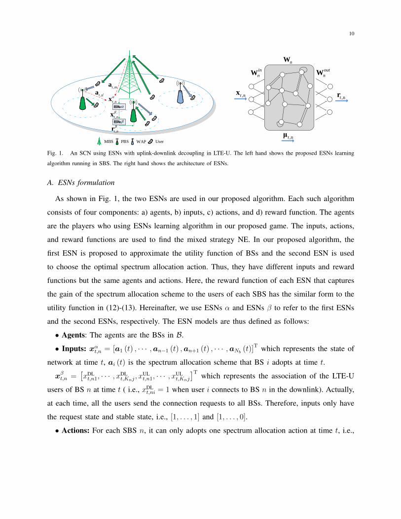
Fig. 1. An SCN using ESNs with uplink-downlink decoupling in LTE-U. The left hand shows the proposed ESNs learning
algorithm running in SBS. The right hand shows the architecture of ESNs.
A. ESNs formulation
As shown in Fig. 1, the two ESNs are used in our proposed algorithm. Each such algorithm
consists of four components: a) agents, b) inputs, c) actions, and d) reward function. The agents
are the players who using ESNs learning algorithm in our proposed game. The inputs, actions,
and reward functions are used to find the mixed strategy NE. In our proposed algorithm, the
first ESN is proposed to approximate the utility function of BSs and the second ESN is used
to choose the optimal spectrum allocation action. Thus, they have different inputs and reward
functions but the same agents and actions. Here, the reward function of each ESN that captures
the gain of the spectrum allocation scheme to the users of each SBS has the similar form to the
utility function in (12)-(13). Hereinafter, we use ESNs α and ESNs β to refer to the first ESNs
and the second ESNs, respectively. The ESN models are thus defined as follows:
• Agents: The agents are the BSs in B.
• Inputs: xαt,n = [a1 (t) , · · · ,an−1 (t) ,an+1 (t) , · · · ,aNb (t)]T which represents the state of
network at time t, ai (t) is the spectrum allocation scheme that BS i adopts at time t.
xβt,n =[xDLt,n1, · · · , xDL
t,Knj, xUL
t,n1, · · · , xULt,Knj
]T which represents the association of the LTE-U
users of BS n at time t ( i.e., xDLt,ni = 1 when user i connects to BS n in the downlink). Actually,
at each time, all the users send the connection requests to all BSs. Therefore, inputs only have
the request state and stable state, i.e., [1, . . . , 1] and [1, . . . , 0].
• Actions: For each SBS n, it can only adopts one spectrum allocation action at time t, i.e.,
11
an (t) = an,i, where an,i ∈ An. Therefore, an,i is specified as follows:
an,i =
di1,n · · · diKn,n, vin,1 · · · vin,Kn
κi1,n · · ·κiKn,n, τin,1 · · · τ in,Kn
T
, (17)
where dij,n is the fraction of the downlink licensed band that SBS n allocates to user j adopting
the spectrum allocation scheme i, vin,j denotes the fraction of the uplink licensed band that SBS
n allocates to user j adopting spectrum allocation scheme i, κij,n and τ in,j respectively, denote
the fractions of the unlicensed band that SBS n allocates to user j in the downlink and uplink.
We consider the case in which each user can access the licensed and unlicensed bands at the
same time. The licensed bandwidths and time slots on the unlicensed band must satisfy (9)-(11).
Thus, an,i represents SBS n adopting spectrums allocation action i to the users. Since the MBS
only has the licensed spectrum to allocate to users, the action of the MBS in An is given by:
am,i =[di1,m · · · diKm,m, v
im,1 · · · vim,Km
]T. (18)
• Reward function: In our model, the vector of reward functions are the functions to
which ESNs approximate. The reward function of ESNs α is used to store the reward of
spectrum allocation action. However, the reward function of ESNs β is used to choose the
optimal spectrum allocation action. Therefore, the reward function is given by rαt,n(xαt,n,An
)=[
rα,1t,n
(xαt,n,an,1
), · · · , rα,|An|t,n
(xαt,n,an,|An|
)]T. rαt,n
(xαt,n,An
)represents the set of spectrum allo-
cation rewards achieved by spectrum allocation schemes for each BS n at time t. According to
(5)-(8), constructing the reward function needs to consider the instability of the unlicensed band
that the WiFi user would occupy at any time. Therefore, the reward function of action i on SBS
n is given by:
rα,it,n(xαt,n,an,i
)= un (an,i,a−n) , (19)
where xαt,n = a−n expresses the input at time t of ESN α is the actions that other BSs adopt at
time t. Since the MBS only has the licensed spectrum to allocate to users, the reward function
of the MBS is given by:
rα,it,m(xαt,m,am,i
)= um (am,a−m) . (20)

12
The reward function in the ESNs β is used to choose the optimal spectrum allocation action
based on the expected reward under the actions that other BSs adopt. It can be expressed by:
rβ,it,n
(xβt,n,an,i
)=
∑xαt,n∈A−n
rα,it,n(xαt,n,an,i
)π−n,xαt,n
(a)=
∑a−n∈A−n
rα,it,n (an,i,a−n)π−n,a−n
= E[rα,it,n (an,i)
], (21)
where (a) is obtained from the fact that the input of the first ESNs xαt,n denotes the actions that
all BSs take at time t other than BS n, i.e., xαt,n = at,−n.
B. ESNs Update
In this subsection, we first introduce the ESNs update that each BS n uses to store and
estimate the reward of each spectrum allocation scheme. Then, we represent the proposed ESN-
based approach that each BS n uses to choose the optimal spectrum allocation scheme. As
shown in Fig. 1, the internal structure of ESNs for BS n consists of three components: a) input
weight matrix W inn , b) recurrent matrix W n, and c) output weight matrix W out
n . Given these
basic definitions, for each BS n, an ESN model is essentially a dynamic neural network, known
as the dynamic reservoir, which will be combined with the input xt,n representing network
state. Therefore, we first explain how an ESN model can be generated. Mathematically, the
dynamic reservoir consists of the input weight matrix W inn ∈ RN×2Kn , and the recurrent matrix
W n ∈ RN×N , where N is the number of units of the dynamic reservoir that each BS n uses
to store the users’ states. The output weight matrix W outn ∈ R|An|×(N+2Kj) is the linear readout
weights which is trained to approximate the reward function of each BS which essentially reflects
the rate achieved by that BS. The dynamic reservoir of BS n is therefore given by the pair(W in
n ,W n
)which is initially generated randomly by uniform distribution and W n is defined
as a sparse matrix with a spectral radius less than one [26]. W outn is also initialized randomly
via a uniform distribution. In this ESN model, one needs to only train W outn to approximate the
reward function which illustrates that ESNs are easy to train [25]–[27]. Even though the dynamic
reservoir is initially generated randomly, it will be combined with input to store the users’ states
and it will also be combined with the trained output matrix to approximate the reward function.
13
Since the users’ associations change depending on the spectrum allocation scheme that each
SBS adopts, the ESN model of each BS n needs to update its input xt,n and store the users’
states, which is done by the dynamic reservoir state µt,n. Here, µt,n denotes the users’ association
results and the users’ states for each BS n at time t. The dynamic reservoir state for each BS
n can be computed as follows:
µjt,n = f(W j
nµjt−1,n +W
j,inn xjt,n
), (22)
where f (·) is the tanh function and j ∈ {α, β}. Suppose that, each BS n, has |An| spectrum
allocation actions, an,1, . . . ,an,|An|, to choose from. Then, the ESNs will have |An| outputs, one
corresponding to each one of those actions. We must train the output matrix W j,outn , so that the
output i yields the value of the reward function rj,it,n(xjt,n,an,i
)due to action an,i in the input
xjt,n:
rj,it,n(xjt,n,an,i
)=W j,out
t,in
[µjt,n;x
jt,n
], (23)
where W j,outt,in denotes the ith row of W j,out
t,n . (23) is used to estimate the reward of each BS
n that adopts any spectrum allocation action after training W j,outn . To train W j,out
n , a linear
gradient descent approach can be used to derive the following update rule:
W j,outt+1,in =W j,out
t,in + λj(ej,it,n − r
j,it,n
(xjt,n,an,i
)) [µjt,n;x
jt,n
]T, (24)
where λj is the learning rate for ESNs j and ej,it,n is the jth actual reward at action i of BS n at
time t, i.e., eα,it,n = uin (an,i,a−n) and eβ,it,n = E [un (an)]. Note that a−n denotes the actions that
all BSs other than BS n adopt now.
C. Reinforcement learning with ESNs algorithm
To solve the game, we introduce the proposed ESN-based reinforcement learning approach to
find the mixed strategy NE. The proposed ESN-based reinforcement learning approach consists
of ESN α and ESN β. ESN α is used to approximate the utility function of our proposed game.
ESN α stores the reward of utility function at any case which can be used by ESN β. ESN
β uses the reward stored in ESN α to find the mixed strategy NE in a reinforcement learning
approach. In our proposed algorithm, each SBS n needs to calculate the number of time slots
L during which SBSs could allocate the unlicensed spectrum based on (8), update the users’
associations and store users’ states based on (22), estimate the rewards of spectrum allocation
14
actions based on (23), choose the optimal allocation scheme, and update the output matrix W outn
based on (24) at each time.
In order to guarantee that any action always has a non-null probability to play in any case, the
ε-greedy exploration [29] is adopted in the proposed algorithm. The mechanism is responsible
for selecting the actions that the agent will perform during the learning process. Its purpose is
to harmonize the tradeoff between exploitation and exploration. Therefore, the probability of BS
n playing action i is given by:
Pr (an (t) = an,i)=
1− ε+ ε|An| , an,i = arg max
an∈Anrβt,n
(xβt,n,an
),
ε|An| , otherwise.
(25)
The ε-greedy mechanism decides the probability distribution of action set for each BS. It can
be easy to conclude that the probability distribution of each SBS’s action set consists of a large
probability of the action that results in the optimal reward and a uniform equal probability for
other actions. Thus, based on ε-greedy mechanism, each BS can obtain the probability distribution
of other BSs’ action sets by only obtaining the spectrum allocation action that results in the
optimal reward.
The learning rates in ESNs have two different rules: a) fixed value and b) the Robbins-Monro
conditions [25]. The Robbins-Monro conditions can be given by:(i) λj (n) > 0,
(ii) limt→∞
t∑n=1
λj (n) = +∞,
(iii) limt→∞
t∑n=1
λ2j (n) < +∞,
(26)
where j ∈ {α, β}. The learning rate has an effect on the speed of the convergence of our proposed
algorithm. However, the two learning rules are all converged with time increases which we would
provide the proof next.
We assume that all BSs transmit simultaneously and each user can only connect to one BS in
the uplink or downlink at each time. We further assume that each SBS knows the time slots that
occupies the unlicensed band L. Based on the above formulations, the distributed RL approach
based on ESNs performed by every BS n is shown in Algorithm 1. In line 8 of Algorithm 1,
we capture the fact that each SBS broadcasts the action that it adopts now and the probability
distribution of action profiles to other BSs.

15
Algorithm 1 Reinforcement learning with ESNs algorithm
Input: The set of users’ association states, xαt,n and xβt,n;
Init: initialize W α,inn , W α
n, W α,outn , W β,in
n , W βn, W β,out
n rα0,n = 0, rβ0,n = 0
1: calculate the time slots L based on (8)
2: for time t do
3: if rand(.) < ε then
4: randomly choose one action
5: else
6: choose action an,i (t) = argmaxan,i(t)
(rβ,it,j
(xβt,n,an,i (t)
))7: end if
8: broadcast the action an,i (t) and the optimal action a∗n that results in the maximal value
of reward function
9: calculate the reward rα and rβ based on (22)-(23)
10: update the output weight matrix W α,outt,ij and W β,out
t,ij based on (24)
11: end for
In essence, at every time instant, every BS allocates its spectrum to the users and maximizes
its own rate. The users would send connection request to all BSs at each time. After iterations,
each user could get the best rate and each BS maximizes its total rate. Note that the performance
of the proposed algorithm can be improved by incorporating a training sequence to update the
output weight matrix W out. Adjusting the input weight matrix W in and recurrent matrix W
appropriately will also improve the accuracy of the algorithm. Algorithm 1 continues to iterate
until each user achieves maximal rate and the users’ association states remain unchanged.
D. Convergence of the ESNs-based algorithm
In the proposed algorithm, we use ESNs α to store and estimate the reward of each spectrum
allocation scheme. Then, we train ESNs β as RL algorithm to solve the proposed game. Since
ESNs have two different learning rules to update the output matrix, in this subsection, we
prove the convergence of the two learning phases of our proposed algorithm. We first prove the
convergence of ESNs with the Robbins-Monro learning rule. Next, we use the continuous time

16
version to prove the convergence of ESNs with the fixed value learning rule. Finally, we prove
the proposed algorithm reaches to the mixed strategy NE.
Theorem 1. ESN α and ESN β for each BS n converge to the utility function un and E [un (an)]
with probability 1 when λj 6= 1/t.
Proof. In order to prove this theorem, we first need to prove the ESNs converges. Then, we
formulate the exact value to which the ESNs converge.
Based on the Gordon’s Theorem [25], the ESNs converge with probability 1 must satisfy: a) a
finite MDP, b) Sarsa learning [30] is being used with a linear function approximator, and c) learn-
ing rates satisfy the Robbins-Monro conditions (λ > 0,∑∞
t=0 λ (t) = +∞,∑∞
t=0 λ2 (t) < +∞).
The proposed game only has two states that are request state and stable state, and the number
of actions is finite which satisfies a).
From (23) and (24), we can formulate the update equation for ESNs as follows:
rj,it+1,n − rj,it,n = λj
(uj,in − r
j,it,n
), j ∈ {α, β} . (27)
Actually, (27) is a special form of Sarsa(0) learning [30]. Condition c) is trivially satisfied via
our learning scheme’s definition. Therefore, we can conclude that the ESNs in our game with
the Robbins-Monro learning rule satisfy Gordon’s Theorem and converge with probability 1.
However, Gordon’s Theorem dose not formulate the exact value to which the ESNs converge.
Therefore, we use the continuous time version of (27) to formulate the exact value to which the
ESNs converges.
To obtain the continuous time version, consider ∆t ∈ [0, 1] to be a small amount of time and
rit+∆t,n−rit,n ≈ ∆t×αt(uit+∆t,n − rit,n
)to be the approximate growth in rin during ∆t. Dividing
both sides of the equation by ∆t and taking the limit for ∆t → 0, (27) can be expressed as
follows:drj,it,ndt≈ λj
(uj,in − r
j,it,n
). (28)
The general solution for (28) can be found by integration:
rj,in = C exp (−λjt) + uj,in , j ∈ {α, β} , (29)
where C is the constant of integration. As exp (−x) is monotonic function and limt→∞ exp (−αtt) =

17
0, when λj 6= 1/t. It is easy to observe that, when t→∞, the limit of (29) is given by:
limt→∞
rj,in =
C exp (−1) + uj,in , λj =1t,
uj,in , λj 6= 1t.
(30)
From (30), we can conclude that the ESNs converge to the utility function as λj 6= 1t, however,
as λj = 1t, the ESNs converge to the utility function with a constant C exp (−1). Moreover, we
can see that the convergence of ESNs actually has no relationship with learning rate, it only
needs enough time to update. This completes the proof.
Theorem 2. The ESN-based algorithm converges to a mixed Nash equilibrium, with the mixed
strategy probability π∗n ∈ ∆ (An), ∀n ∈ B.
Proof. In order to prove Theorem 2, we need to establish the mixed NE conditions in (15). We
assume that the spectrum allocation action a∗n results in the optimal reward given the optimal
mixed strategy (π∗n,π∗−n), which means that π∗n,a∗n = 1−ε+ ε
|An| and π∗n,a′n = ε|An| . We also assume
that an ∈ An/a∗n results in the optimal reward given the optimal mixed strategy (πn,π∗−n). Based
on the Theorem 1, ESN β of the proposed algorithm converges to E [un (an)]. Thus, (15) can
be rewritten as follows:
un(π∗n,π
∗−n)− un
(πn,π
∗−n)
=∑
an∈An
π∗n,an ∑a−n∈A−n
un (an,a−n) π∗n,a−n − πn,an
∑a−n∈A−n
un (an,a−n) π∗n,a−n
=∑
an∈An
[π∗n,anE [un (an)]− πn,anE [un (an)]
](a)= (1− ε) (E [un (a
∗n)]− E [un (an)]) (31)
where (a) is obtained from the fact that π∗n,a∗n = πn,an = 1− ε+ ε|An| and π∗n,a′n = πn,a′′n = ε
|An| ,
a′n ∈ An/a∗n, a′′n ∈ An/an. Since in our proposed algorithm, the optimal action a∗n results in
the optimal E [un (a∗n)], we can conclude that E [un (a
∗n)]− E [un (an)] ≥ 0. This completes the
proof.
IV. SIMULATION RESULTS
In this section, we evaluate the performance of the proposed ESN algorithm using simulations.
We first introduce the simulation parameters. Further, we evaluate the performance of ESNs’

18
approximation and estimation in our proposed algorithm. Finally, we show the improvements
in terms of sum-rate of all users and the 50th percentile of users by comparing the proposed
algorithm with three Q-learning algorithms.
A. System Parameters
For our simulations, we use the following parameters. One macrocell with a radius rM = 500
meters is considered with Ns uniformly distributed picocells, W = 2 uniformly distributed WiFi
access points, and U uniformly distributed LTE-U users. The picocells share the licensed band
with MBS and the unlicensed band with WiFi. Each WAP has 4 WiFi users. The channel gain is
generated as Rayleigh variables with unit variance. The WiFi network is set up based on the IEEE
802.11n protocol working at the 5 GHz band with a RTS/CTS mechanism. Other parameters
are listed in Table I. The results are compared to three schemes: a) Q-learning with uplink-
downlink decoupling, b) Q-learning with uplink-downlink decoupling within an LTE system,
and c) Q-learning without uplink-downlink decoupling. All statistical results are averaged over
a large number of independent runs. Hereinafter, we use the term “sum-rate” to refer to the total
downlink and uplink rates and “Q-learning" to refer to the Q-learning with uplink-downlink
decoupling within an LTE-U system.
We assume Q-learning in our simulations has knowledge of the action that each BS takes and
the entire users’ information including interference and location. The update rule of Q-learning
can be expressed as follows:
Qit+1 = (1− λq)Qi
t + λq(an,i,a
∗−n), (32)
where a∗−n represents the optimal action profile of all BSs other than SBS n.
B. ESNs Approximation
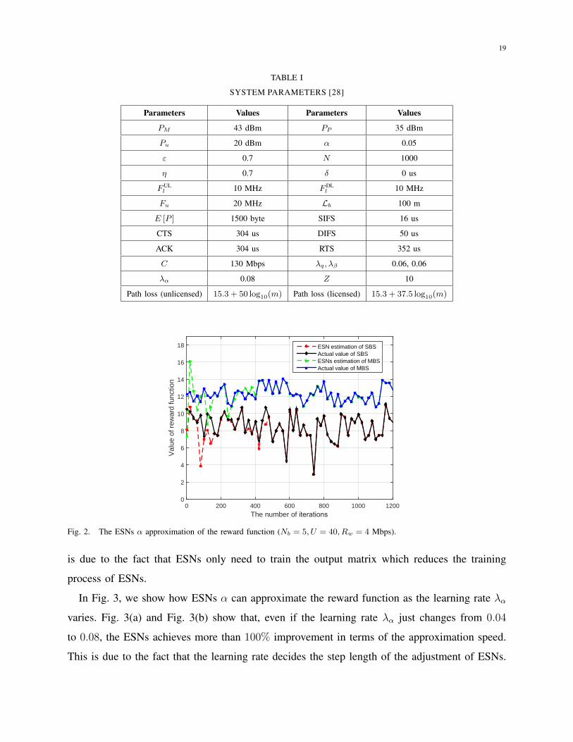
Fig. 2 shows how the first ESNs approximate to the reward function as the number of iteration
varies. In Fig. 2, we can see that, as the number of iteration increases, the approximations of
BSs improve. This demonstrates the effectiveness of ESN as an approximation tool for utility
functions. Moreover, the network state stored in the ESNs improves the approximation which
records the value of reward function according to the network state. Fig. 2 also shows that the
ESNs only need less than 100 iterations to finish the approximation of the reward function. This
19
TABLE I
SYSTEM PARAMETERS [28]
Parameters Values Parameters Values
PM 43 dBm PP 35 dBm
Pu 20 dBm α 0.05
ε 0.7 N 1000
η 0.7 δ 0 us
FULl 10 MHz FDL
l 10 MHz
Fu 20 MHz Lb 100 m
E [P ] 1500 byte SIFS 16 us
CTS 304 us DIFS 50 us
ACK 304 us RTS 352 us
C 130 Mbps λq, λβ 0.06, 0.06
λα 0.08 Z 10
Path loss (unlicensed) 15.3 + 50 log10(m) Path loss (licensed) 15.3 + 37.5 log10(m)
The number of iterations0 200 400 600 800 1000 1200
Val
ue o
f rew
ard
func
tion
0
2
4
6
8
10
12
14
16
18 ESN estimation of SBSActual value of SBSESNs estimation of MBSActual value of MBS
Fig. 2. The ESNs α approximation of the reward function (Nb = 5, U = 40, Rw = 4 Mbps).
is due to the fact that ESNs only need to train the output matrix which reduces the training
process of ESNs.
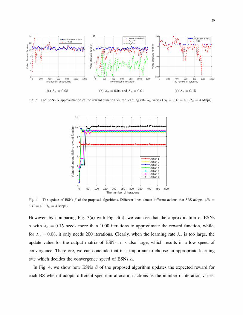
In Fig. 3, we show how ESNs α can approximate the reward function as the learning rate λα
varies. Fig. 3(a) and Fig. 3(b) show that, even if the learning rate λα just changes from 0.04
to 0.08, the ESNs achieves more than 100% improvement in terms of the approximation speed.
This is due to the fact that the learning rate decides the step length of the adjustment of ESNs.
20
The number of iterations0 200 400 600 800 1000 1200
Val
ue o
f rew
ard
func
tion
2
4
6
8
10
12
14
Actual value of MBS6,=0.08
(a) λα = 0.08
The number of iterations0 200 400 600 800 1000 1200
Val
ue o
f rew
ard
func
tion
0
5
10
15Actual value of MBS6,=0.04
6,=0.01
(b) λα = 0.04 and λα = 0.01
The number of iterations0 200 400 600 800 1000 1200
Val
ue o
f rew
ard
func
tion
-150
-100
-50
0
50Actual value of MBS6,=0.15
(c) λα = 0.15
Fig. 3. The ESNs α approximation of the reward function vs. the learning rate λα varies (Nb = 5, U = 40, Rw = 4 Mbps).
The number of iterations0 50 100 150 200 250 300 350 400 450 500
Val
ue o
f sec
ond
ES
Ns
rew
ard
func
tion
-2
0
2
4
6
8
10
12
Action 1Action 2Action 3Action 4Action 5Action 6Action 7
Fig. 4. The update of ESNs β of the proposed algorithms. Different lines denote different actions that SBS adopts. (Nb =
5, U = 40, Rw = 4 Mbps).
However, by comparing Fig. 3(a) with Fig. 3(c), we can see that the approximation of ESNs
α with λα = 0.15 needs more than 1000 iterations to approximate the reward function, while,
for λα = 0.08, it only needs 200 iterations. Clearly, when the learning rate λα is too large, the
update value for the output matrix of ESNs α is also large, which results in a low speed of
convergence. Therefore, we can conclude that it is important to choose an appropriate learning
rate which decides the convergence speed of ESNs α.
In Fig. 4, we show how ESNs β of the proposed algorithm updates the expected reward for
each BS when it adopts different spectrum allocation actions as the number of iteration varies.

21
In this figure, each line of ESNs β stands for one spectrum allocation action of each BS. We
can see that each line of ESNs β converges to a stable value as the number of iteration increases
which implies that by using ESNs, each BS can estimate the reward before BS takes any action.
This is due to the fact that, as iteration increases, the approximation of ESNs α provides the
reward that ESNs β can be used to calculate the expected reward. Fig. 4 also shows that, as
below iteration 100, the expected reward of each spectrum allocation action changes quickly.
However, each curve exhibits only small oscillations as the number of iterations is more than
100. The main reason behind this is that, at the beginning, ESN α spends some iterations to
approximate the reward function. Since the ESNs α has not yet approximated the reward function
well, ESNs β can not calculate the expected reward for each action accurately. As the number
of iterations is above 100, ESNs α finishes the approximation of reward function, which results
in the accurate calculation of expected reward for ESNs β.
Fig. 5 shows the cumulative distribution function (CDF) of rate in both the uplink and downlink
for all the considered schemes. In Fig. 5(a), we can see that, the uplink rates of 6%, 9%, 10%, and
15% users from all the considered algorithm are below 0.001 Mbps. This is due to the fact that,
in all considered algorithms, each SBS has a limited coverage which limits users’ associations.
The coverage results in the users who are far away from the MBS but not in the coverage of
any SBS associating with the MBS. Fig. 5(a) also shows that the proposed approach improves
the uplink CDF at low rate yielding up to 50% and 130% gains for 0.001 Mbps rate compared
to Q-learning and Q-learning without decoupling, respectively. This is due to the fact that the
proposed algorithm chooses the action based on the expected reward which is calculated by two
ESNs to update but Q-learning only uses the maximal reward to choose action and both the
proposed approach and Q-learning adopt uplink-downlink decoupling to improve their uplink
rates. Fig. 5(b) also shows that the proposed approach improves the downlink CDF at low rate
showing 150%, 25%, and 5% gains for 0.05, 0.5 and 5 Mbps rates compared to the Q-learning.
This is because the proposed approach uses the estimated expected value of the reward function
to choose the optimal allocation scheme that results in the optimal reward.
In Fig. 6, we show how the total sum-rate varies with the number of SBSs. In Fig. 6(a),
we can see that, as the number of SBSs increases, all algorithms result in increasing sum-rates
because the users have more choices to choose an SBS and the distances from the SBSs to the
users decrease. Fig. 6(a) also shows that Q-learning achieves, respectively, up to 7% and 20%

22
Uplink user rate (Mbps)0.001 0.005 0.01 0.05 0.1 0.5 1 5 10 15
CD
F
0
0.1
0.2
0.3
0.4
0.5
0.6
0.7
0.8
0.9
1
Proposed ESN algorithmQ-learning algorithmQ-learning in LTEQ-learning without decoulping
(a)
Downlink user rate (Mbps)0.005 0.05 0.5 1 5 10 15 20 30 50
CD
F
0
0.1
0.2
0.3
0.4
0.5
0.6
0.7
0.8
0.9
1
Proposed ESN algorithmQ-learning algorithmLTE Q-learningQ-learning without decoulping
(b)
Fig. 5. Downlink and uplink rates CDFs resulting from the different algorithms (U = 40, Ns = 5, Rw = 4 Mbps).
improvements in the sum-rate compared to Q-learning within an LTE system and Q-learning
without decoupling for the case with 8 SBSs. Clearly, downlink-uplink decoupling and LTE
utilizing unlicensed band improve the network performance. However, Fig. 6(b) shows that the
rates of the 50th percentile of users decreases as the number of SBSs increases. This is due to
the fact that, in our simulations, each SBS has a limited coverage area that restricts the access

23
Number of SBSs3 4 5 6 7 8
Sum
-rat
e of
use
rs (
Mbp
s)
150
200
250
300
350
400
450
500
Proposed ESN algorithmQ-learning algorithmQ-learning in LTEQ-learning without decoulping
(a)
Number of SBSs3 4 5 6 7 8
Sum
-rat
e of
50t
h pe
rcen
tile
user
s (M
bps)
1
2
3
4
5
6
7
8
Proposed ESN algorithmQ-learning algorithmQ-learning in LTEQ-learning without decoulping
(b)
Fig. 6. Sum-rate as the number of SBSs varies (U = 40, Rw = 4 Mbps).
of the users who are located far away from the MBS and not in the coverage of any SBS. Thus,
as the number of SBSs increase, the interference to the limited users are increased which results
in the decrease of the 50th percentile of users’ throughput. By comparing Fig. 6(a) with Fig.
6(b), we can also see that the proposed approach achieves, respectively, 3% and 19.5% gains of
sum-rate, and 60% and 78% gains of the sum-rate of the 50th percentile of users compared to

24
Number of users20 30 40 50 60 70 80
Sum
-rat
e of
use
rs (
Mbp
s)
180
200
220
240
260
280
300
320
340Proposed ESN algorithmQ-learning algorithmQ-learning in LTEQ-learning without decoulping
(a) Sum-rates of all users
Number of users20 30 40 50 60 70 80
Sum
-rat
e of
50t
h pe
rcen
tile
user
s (M
bps)
1
2
3
4
5
6
7
8
Proposed ESN algorithmQ-learning algorithmQ-learning in LTEQ-learning without decoulping
(b) Sum-rates of the 50th percentile of users
Fig. 7. Downlink and uplink sum-rates of users vs. the number of users (Ns = 4, Rw = 4 Mbps).
Q-learning for the case with 8 SBSs. This demonstrates that the proposed algorithm balances
the load better than Q-learning, which allocates appropriate spectrum to the users who have low
SINRs. Moreover, Fig. 6(a) and Fig. 6(b) also show that the Q-learning in LTE has a higher
sum rate of the 50th percentile of users but lower sum-rate of all users than Q-learning without
decoupling. It is obvious that the downlink-uplink decoupling improves the rate of edge users.
25
The rate requirement of WiFi users (Mbps) 1 2 3 4 5 6
Sum
-rat
e of
use
rs (
Mbp
s)
200
250
300
350
400
450
500
Proposed ESN algorithmQ-learning algorithmQ-learning in LTEQ-learning without decoulping
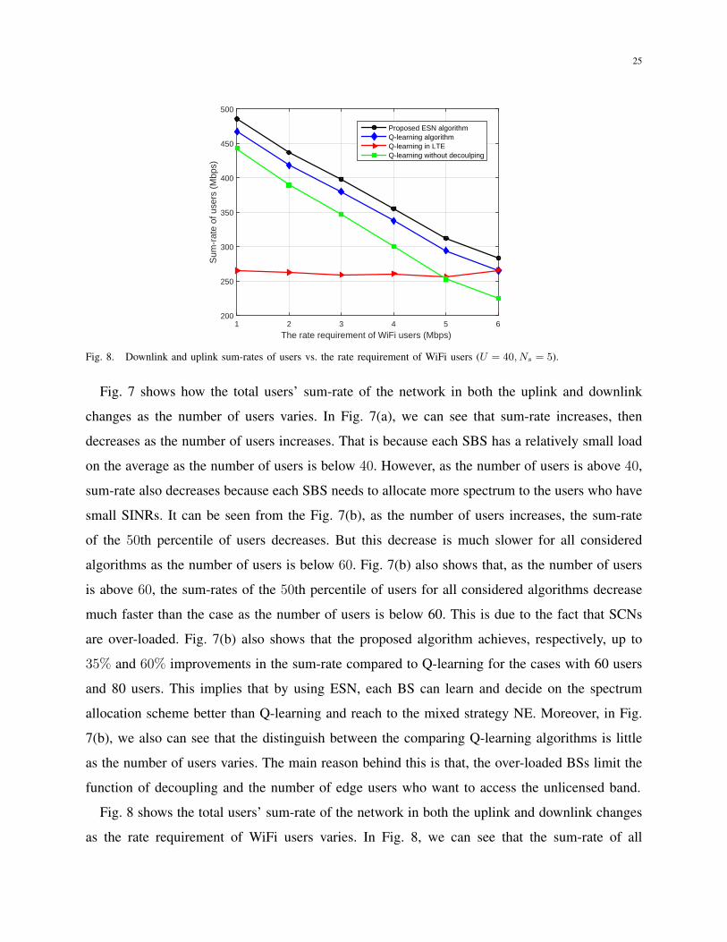
Fig. 8. Downlink and uplink sum-rates of users vs. the rate requirement of WiFi users (U = 40, Ns = 5).
Fig. 7 shows how the total users’ sum-rate of the network in both the uplink and downlink
changes as the number of users varies. In Fig. 7(a), we can see that sum-rate increases, then
decreases as the number of users increases. That is because each SBS has a relatively small load
on the average as the number of users is below 40. However, as the number of users is above 40,
sum-rate also decreases because each SBS needs to allocate more spectrum to the users who have
small SINRs. It can be seen from the Fig. 7(b), as the number of users increases, the sum-rate
of the 50th percentile of users decreases. But this decrease is much slower for all considered
algorithms as the number of users is below 60. Fig. 7(b) also shows that, as the number of users
is above 60, the sum-rates of the 50th percentile of users for all considered algorithms decrease
much faster than the case as the number of users is below 60. This is due to the fact that SCNs
are over-loaded. Fig. 7(b) also shows that the proposed algorithm achieves, respectively, up to
35% and 60% improvements in the sum-rate compared to Q-learning for the cases with 60 users
and 80 users. This implies that by using ESN, each BS can learn and decide on the spectrum
allocation scheme better than Q-learning and reach to the mixed strategy NE. Moreover, in Fig.
7(b), we also can see that the distinguish between the comparing Q-learning algorithms is little
as the number of users varies. The main reason behind this is that, the over-loaded BSs limit the
function of decoupling and the number of edge users who want to access the unlicensed band.
Fig. 8 shows the total users’ sum-rate of the network in both the uplink and downlink changes
as the rate requirement of WiFi users varies. In Fig. 8, we can see that the sum-rate of all

26
Number of iterations0 100 200 300 400 500 600 700 800 900 1000
Val
ue o
f rew
ard
func
tion
0
10
20
30
40
50
60
70
80
90
Proposed ESN algorithmQ-learning algorithm
(a) The case with convergence of Q-learning
Number of iterations0 100 200 300 400 500 600 700 800 900 1000
Val
ue o
f rew
ard
func
tion
0
10
20
30
40
50
60
70
80
90
100 Proposed ESN algorithmQ-learning algorithm
(b) The case with divergence of Q-learning
Fig. 9. The convergence of the algorithms (Ns = 5, U = 40, Rw = 4 Mbps).
considered algorithms other than the Q-learning in LTE decrease as the rate requirement of
WiFi users increases. That is because the time of unlicensed spectrum that BSs can occupy
decreases as the rate requirement of WiFi users increases. Fig. 8 also shows that Q-learning
without decoupling has lower sum-rate compared to Q-learning in LTE as the case with the rate
requirement of WiFi users is above 5 Mbps. This is due to the fact that Q-learning in LTE-U

27
Number of SBSs3 4 5 6 7 8
Itera
tions
400
450
500
550
600
650
700
750
800
with 40 userswith 80 users
Fig. 10. The convergence time of the proposed algorithm as a function of the number of SBSs (Rw = 4 Mbps).
without decoupling becomes Q-learning in LTE without decoupling.
Fig. 9 shows the number of iterations needed till convergence for both the proposed approach
and Q-learning. In this figure, we can see that, as time elapses, the total value of reward function
increase until convergence to their final values. In Fig. 9(a) , we can see that, the proposed
approach needs 300 iterations to reach convergence and exhibits an acceptable increase of
iterations compared to Q-learning. The main reason behind this is because Q-learning exploits
the entire informations of all users and BSs to update the Q-table, but the proposed algorithm
only needs the action informations of BSs to update output matrix. However, Fig. 9(b) shows
that the proposed algorithm reaches convergence as the iteration increases but the Q-learning
diverges. Moreover, the proposed algorithm achieves up to 60% improvement compared to Q-
learning. This is due to the fact that ESN-based learning stores the users’ states and actions
of BSs to calculate the expected value of each action of BSs which guarantees the proposed
algorithm to reach the mixed strategy NE. Note that, since Q-learning would diverge in some
cases, we choose the maximal value as the converge point in the case that Q-learning diverges.
In Fig. 10, we show the convergence time of the proposed approach as the number of SBSs
varies for 40 and 80 users. In this figure, we can see that, as the network size increases, the
average number of iterations till convergence increases. Fig. 10 also shows that reducing the
number of users leads to a faster convergence time. Although users are not players in the game,
they affect spectrum allocation action selection for each BS. As the number of users increases,

28
the spectrum allocation action for each BS increases, and, thus, a longer convergence time is
observed.
V. CONCLUSION
In this paper, we have developed a novel resource allocation framework for optimizing the
use of uplink-downlink decoupling in an LTE-U system. We have formulated the problem as
a noncooperative game between the BSs that seeks to maximize the total uplink and downlink
rates while balancing the load among one another. To solve this game, we have developed a
novel algorithm based on the machine learning tools of echo state networks. The proposed
algorithm enables each BS to decide on its spectrum allocation scheme autonomously with
limited information on the network state. Simulation results have shown that the proposed
approach yields significant performance gains in terms of rate and load balancing compared
to conventional approaches. Moreover, the results have also shown that the use of ESN can
significantly reduce the information exchange for the wireless networks.
REFERENCES
[1] Cisco, “Cisco visual networking index: Global mobile data traffic forecast update 2014-2019,” Whitepaper, Feb. 2015.
[2] F. Boccardi, J. G. Andrews, H. Elshaer, M. Dohler, S. Parkvall, P. Popovski, and S. Singh, “Why to decouple the uplink
and downlink in cellular networks and how to do it,” arXiv preprint arXiv:1503.06746, March 2015.
[3] S. Singh, X. Zhang, and J. G. Andrews, “Joint rate and SINR coverage analysis for decoupled uplink-downlink biased
cell associations in hetnets,” IEEE Transactions on Wireless Communications, vol. 14, no. 10, pp. 5360–5373, April 2015.
[4] F. Liu, E. Bala, E. Erkip, M. Beluri, and R. Yang, “Small cell traffic balancing over licensed and unlicensed bands,” IEEE
Transactions on Vehicular Technology, vol. 64, no. 12, pp. 5850–5865, Jan. 2015.
[5] K. Xin, Y. K. Chia, S. Sun, and H. F. Chong, “Mobile data offloading through a third-party WiFi access point: An
operator’s perspective,” IEEE Transactions on Wireless Communications, vol. 13, no. 10, pp. 5340–5351, Oct. 2014.
[6] O. Galinina, A. Pyattaev, S. Andreev, M. Dohler, and Y. Koucheryavy, “5G multi-rat LTE-WiFi ultra-dense small cells:
Performance dynamics, architecture, and trends,” IEEE Journal on Selected Areas in Communications, vol. 33, no. 6, pp.
1224–1240, Mar. 2015.
[7] M. R Khawer, J. Tang, and F. Han, “usICIC-A proactive small cell interference mitigation strategy for improving spectral
efficiency of LTE networks in the unlicensed spectrum,” IEEE Transactions on Wireless Communications, to appear.
[8] A. R. Elsherif, W. Chen, A. Ito, and Zhi Ding, “Resource allocation and inter-cell interference management for dual-access
small cells,” IEEE Journal on Selected Areas in Communications, vol. 33, no. 6, pp. 1082–1096, Mar. 2015.
[9] A. Kumar, A. Sengupta, R. Tandon, and T.C. Clancy, “Dynamic resource allocation for cooperative spectrum sharing in
LTE networks,” IEEE Transactions on Vehicular Technology, vol. 64, no. 11, pp. 5232–5245, Dec. 2014.
[10] F. Liu, Erdem Bala, Elza Erkip, M. C. Beluri, and Rui Yang, “Small cell traffic balancing over licensed and unlicensed
bands,” arXiv preprint arXiv:1501.00203, Dec. 2014.
29
[11] R. Zhang, M. Wang, L. Cai, Z. Zheng, X. Shen, and L. Xie, “LTE-unlicensed: The future of spectrum aggregation for
cellular networks,” IEEE Wireless Communications, vol. 22, no. 3, pp. 150–159, June 2015.
[12] D. Fudenberg and D. K. Levine, “The theory of learning in games,” General Information, vol. 133, no. 1, pp. 177–198,
1996.
[13] Y. Hu, G. Yang, and A. Bo, “Multiagent reinforcement learning with unshared value functions,” IEEE Transactions on
Cybernetics, vol. 45, no. 4, pp. 647–662, July 2014.
[14] H. Li, “Multi-agent Q-learning of channel selection in multi-user cognitive radio systems: a two by two case,” in Proc.
of IEEE International Conference on Systems, Man and Cybernetics (SMC), San Antonio, TX, 2009.
[15] D. Niyato and E. Hossain, “Dynamic of network selection in heterogeneous wireless networks: an evolutionary game
approach,” IEEE Transactions on Vehicular Technology, vol. 58, no. 4, pp. 2008–2017, Aug. 2008.
[16] M. Bennis and S. M. Perlaza, “Decentralized cross-tier interference mitigation in cognitive femtocell networks,” in Proc.
of IEEE International Conference on Communications (ICC), Kyoto, June 2011.
[17] S. Samarakoon, M. Bennis, W. Saad, and M. Latva-aho, “Backhaul-aware interference management in the uplink of
wireless small cell networks,” IEEE Transactions on Wireless Communications, vol. 12, no. 11, pp. 5813–5825, Sept.
2013.
[18] S. Samarakoon, M. Bennis, W. Saad, and M. Latva-aho, “Dynamic clustering and on/off strategies for wireless small cell
networks,” IEEE Transactions on Wireless Communications, to appear.
[19] S. Samarakoon, M. Bennis, W. Saad, and M. Latva-aho, “Opportunistic sleep mode strategies in wireless small cell
networks,” in Proc. of IEEE International Conference on Communications (ICC), Sydney, NSW, 2014.
[20] M. Bennis, S.M. Perlaza, P. Blasco, Z. Han, and H.V. Poor, “Self-organization in small cell networks: A reinforcement
learning approach,” IEEE Transactions on Wireless Communications, vol. 12, no. 7, pp. 3202–3212, June 2013.
[21] L. Busoniu, R. Babuska, and B. De Schutter, “A comprehensive survey of multiagent reinforcement learning,” IEEE
Transactions on Systems, Man, and Cybernetics, vol. 38, no. 2, pp. 156–172, March 2008.
[22] K. Bush and C. Anderson, “Modeling reward functions for incomplete state representations via echo state networks,” in
Proc. of IEEE International Joint Conference on Neural Networks (IJCNN), Piscataway, NJ, July 2005.
[23] A. Anderson and H. Haas, “Using echo state networks to characterise wireless channels,” in Proc. of Vehicular Technology
Conference (VTC Spring), Dresden, Germany, June 2013.
[24] M. Bauduin, A. Smerieri, S. Massar, and F. Horlin, “Equalization of the non-linear satellite communication channel with
an echo state network,” in Proc. of Vehicular Technology Conference (VTC Spring), Glasgow, Scotland, May 2015.
[25] I. Szita, V. Gyenes, and A. Lorincz, “Reinforcement learning with echo state networks,” Lecture Notes in Computer
Science, vol. 4131, pp. 830–839, 2006.
[26] Mantas Lukosevicius, A Practical Guide to Applying Echo State Networks, Springer Berlin Heidelberg, 2012.
[27] K. C. Chatzidimitriou, L. Partalas, P. A. Mitkas, and L. Vlahavas, “Transferring evolved reservoir features in reinforcement
learning tasks,” European Conference on Recent Advances in Reinforcement Learning, 2011.
[28] G. Bianchi, “Performance analysis of IEEE 802.11 distributed coordination function,” IEEE Journal on Selected Areas in
Communications, vol. 18, no. 3, pp. 535–547, March 2000.
[29] M. Bennis and D. Niyato, “A Q-learning based approach to interference avoidance in self-organized femtocell networks,”
in Proc. of IEEE Global Commun. Conference (GLOBECOM) Workshop on Femtocell Networks, Miami, FL, USA, Dec.
2010.
[30] R. Sutton and A. Barto, Reinforcement Learning:An Introduction, MIT Press, 1998.