Bipolar Junction Transistors (BJT) NPNPNP. BJT Cross-Sections NPN PNP Emitter Collector.

ECEN 326 LAB 1Design of a Common-Emitter BJT Amplifier
1 Circuit Topology and Design Equations
General configuration of a single-supply common-emitter BJT amplifier is shown in Fig. 1.
CB
Rin
Isupply
I1
Q1
RE
IB
RC(1−k)RB
kRB
VCC
VE
VC
CC
CE
RG
RL
Vout
Vin
Figure 1: Common-Emitter BJT Amplifier
For β-insensitive DC biasing, the base current (IB) should be negligible compared to I1:
IB I1 ⇒ IC
β VCC
RB⇒ N
IC
β=
VCC
RB⇒ RB =
βVCC
NIC, N ≥ 10 (1)
Small-signal AC voltage gain (Av) can be expressed as
Av =∣∣∣∣vout
vin
∣∣∣∣ =RC ‖ RL
re + (RE ‖ RG)⇒ re + (RE ‖ RG) =
RC ‖ RL
Av(2)
Input resistance of the amplifier (Rin) is usually included in the given specifications. It can be calculated as
Rin = kRB ‖ (1− k)RB ‖ (β + 1)[re + (RE ‖ RG)] ≈ k(1− k)RB ‖ β[re + (RE ‖ RG)] (3)
Substituting RB from (1) and [re + (RE ‖ RG)] from (2) into (3) results in
Rin =(
k(1− k)βVCC
NIC
)‖
(β
RC ‖ RL
Av
)=
βNIC
k(1− k)VCC+
Av
RC ‖ RL
(4)
To maximize the available output swing, load-line analysis needs to be performed. Assume that the transistor’s DCoperating point is set to (IC , VCE). The following equation can be obtained from the DC equivalent circuit of Fig. 1
VCC = ICRC + VCE + VE ⇒ VCE = VCC − ICRC − VE (5)
AC load line, which shows the relationship between the AC signals ic and vce, passes through the DC bias point(IC , VCE). The slope of the line depends on the AC resistance at the collector and emitter terminals. For the common-emitter amplifier circuit in Fig. 1, the slope can be found as
∆ic∆vce
= − 1(RC ‖ RL) + (RE ‖ RG)
(6)
1

symmetrical swing
c
VCE,sat
vce
DC bias point
−VCE,sat2VCE
VCE
IC
0
For maximum
i
Figure 2: AC load line
Therefore, the load line equation can be obtained as
ic − IC
vce − VCE= − 1
(RC ‖ RL) + (RE ‖ RG)(7)
To obtain the maximum symmetrical swing, the DC bias point should be at the middle of the available region. Sincethe minimum value for vce is VCE,sat, the maximum value of vce corresponding to ic = 0 should be (2VCE−VCE,sat),as shown in Fig. 2. Evaluating the load-line equation at the point (ic, vce) = (0, 2VCE − VCE,sat),
0− IC
2VCE − VCE,sat − VCE= − 1
(RC ‖ RL) + (RE ‖ RG)(8)
which can be arranged asIC [(RC ‖ RL) + (RE ‖ RG)] = VCE − VCE,sat (9)
Substituting VCE from (5) into (9) results in
IC [(RC ‖ RL) + (RE ‖ RG)] = VCC − ICRC − VE − VCE,sat (10)
which can be arranged as
IC =VX
RC + (RC ‖ RL) + (RE ‖ RG)(11)
whereVX = VCC − VE − VCE,sat (12)
From (2), Av 1 implies (RC ‖ RL) (RE ‖ RG). Therefore, (11) can be simplified as
IC ≈VX
RC + (RC ‖ RL)(13)
0-to-peak voltage swing can be calculated as
Vsw = IC(RC ‖ RL) =VX
2 +RC
RL
(14)
Substituting IC in (13) into (4), Rin can be expressed as
Rin =β(RC ‖ RL)
NVX
k(1− k)VCC
1
2 +RC
RL
+ Av
(15)
2

2 Design Procedure
1. VCC , VCE,sat and β should be given together with the design specifications, which usually include Rin, Av ,0-to-peak output swing (Vsw), and RL. In addition, the design should be insensitive to variations in β and VBE .
2. First, choose the value of VE . Increasing VE results in more stable bias current in the presence of VBE variations,however it decreases the available voltage swing at the collector. If the resistor RE is replaced with a DC currentsource, VE should be sufficiently large to allow proper operation of the source.
3. Calculate VX and k as follows
VX = VCC − VCE,sat − VE , k =VE + 0.7
VCC
Also choose N such that N ≥ 10.
4. Determine the minimum value of RC using the specification for the desired input resistance (Rin,d):
β(RC ‖ RL)NVX
k(1− k)VCC
1
2 +RC
RL
+ Av
≥ Rin,d
which can be arranged as
R2C(βRL −Rin,dAv) + RC(2βRL − 3Rin,dAv −QRin,d)RL −R2
LRin,d(Q + 2Av) ≥ 0
whereQ =
NVX
k(1− k)VCC
5. Determine the maximum value of RC using the specification for the desired output voltage swing (Vsw,d):
VX
2 +RC
RL
≥ Vsw,d
which can be arranged as
RC ≤ RL
(VX
Vsw,d− 2
)6. Choose RC , then calculate IC
IC ≈VX
RC + (RC ‖ RL)
7. Calculate RB and RE
RB =βVCC
NIC, RE =
VE
IC
8. Find RG from
re + (RE ‖ RG) =RC ‖ RL
Av
which can be arranged as
RG =1
1(RC ‖ RL
Av− re
) − 1RE
3

3 Pre-Lab
Using a Q2N2222 BJT, design a common-emitter amplifier with the following specifications:
VE ≥ 1 V Rin ≥ 5 kΩ 0-to-peak unclipped swing at Vout ≥ 1.6 VVCC = 5 V |Av| = 40 Operating frequency: 5 kHzRL = 10 kΩ Isupply ≤ 1.5 mA
1. Show all your calculations and final component values.
2. Verify your results using PSPICE. Submit all necessary simulation plots showing that the specifications aresatisfied. Also provide the circuit schematic with DC bias points annotated.
3. Using PSPICE, perform Fourier analysis and determine the input and the output signal amplitudes resulting in5% total harmonic distortion (THD) at the output. Submit transient and Fourier plots, and the distortion datafrom the output file.
4. Be prepared to discuss your design at the beginning of the lab period with your TA.
4 Lab Procedure
1. Construct the common-emitter amplifier you designed in the pre-lab.
2. Measure IC , VE , VC and VB . If any DC bias value is significantly different than the one obtained from Pspicesimulations, modify your circuit to get the desired DC bias before you move onto the next step.
3. Measure Isupply , Av , Rin, and Rout.
4. Measure the maximum unclipped output signal amplitude.
5. Apply the input signal level resulting in 5% THD at the output, and measure the input and output signal ampli-tudes.
6. Prepare a data sheet showing your simulated and measured values.
7. Be prepared to discuss your experiment with your TA. Have your data sheet checked off by your TA beforeleaving the lab.
4

ECEN 326 LAB 2Design of a Three-Stage BJT Amplifier
1 Circuit Topology and Design Equations
Figure 1 shows the three-stage amplifier to be designed in this lab. The first stage is a common-emitter amplifier,which is followed by a common-base stage. This combination is known as the cascode amplifier. An emitter followeris added as the final stage.
b3
RC
RB4
Q1
Q3Q2
Isupply
Rin
v
vin
RL
vout
Ri2
VE2
RB3
Ri3
IQioutRGREkRB
VCC (1−k)RB
IB1
I1I3
Figure 1: Cascode amplifier with an emitter follower
For β-insensitive DC biasing, the base current of Q1 (IB1) should be negligible compared to I1:
IB1 I1 ⇒ IC1
β VCC
RB⇒ N
IC1
β=
VCC
RB⇒ RB =
βVCC
NIC1, N ≥ 10 (1)
Small-signal AC voltage gain (Av) can be expressed as
Av =∣∣∣∣vout
vin
∣∣∣∣ =Ri2
re1 + (RE ‖ RG)RC ‖ Ri3
Ri2AF ⇒ re1 + (RE ‖ RG) =
RC ‖ Ri3
AvAF (2)
where
AF =vout
vb3=
RL
re3 + RL(3)
Ri3 = (β + 1)(re3 + RL) (4)
Input resistance of the amplifier (Rin) can be calculated as
Rin = kRB ‖ (1− k)RB ‖ (β + 1)[re1 + (RE ‖ RG)] ≈ k(1− k)RB ‖ β[re1 + (RE ‖ RG)] (5)
Substituting RB from (1) and [re1 + (RE ‖ RG)] from (2) into (5) results in
Rin =(
k(1− k)βVCC
NIC1
)‖
(β
RC ‖ Ri3
AvAF
)=
βNIC1
k(1− k)VCC+
Av
(RC ‖ Ri3)AF
(6)
The small-signal AC voltage gain from vin to ve2 is less than unity. Therefore, the AC signal swing at ve2 can beassumed to be limited by the maximum input signal amplitude (Vi,max), which can be calculated by dividing therequired output swing to the gain specification. To avoid clipping at ve2, the DC bias at VE2 can be chosen as
VE2 ≥ VE1 + VCE,sat + Vi,max (7)
To maximize the available output swing, load-line analysis needs to be performed. Assume that Q2’s DC operatingpoint is set to (IC2, VCE2). From Fig. 1
VCC ≈ IC2RC + VCE2 + VE2 ⇒ VCE2 = VCC − IC2RC − VE2 (8)
1

Please note that the above expression is valid only if IC2 IB3. Since IC3 is usually a large current, this requirementusually determines the minimum amount of IC2. AC load line equation for Q2 (see Fig. 2) can be obtained as
ic2 − IC2
vce2 − VCE2≈ − 1
RC ‖ Ri3(9)
symmetrical swing
c2
VCE,sat
vce2
DC bias point
VCE2
−VCE,sat2VCE2
IC2
0
For maximum
i
Figure 2: AC load line
Evaluating the load-line equation at the point (ic2, vce2) = (0, 2VCE2 − VCE,sat),
0− IC2
2VCE2 − VCE,sat − VCE2= − 1
RC ‖ Ri3(10)
which can be arranged asIC2(RC ‖ Ri3) = VCE2 − VCE,sat (11)
Substituting VCE2 from (8) into (11) results in
IC2 =VX
RC + (RC ‖ Ri3)= IC1 (12)
whereVX = VCC − VE2 − VCE,sat (13)
0-to-peak voltage swing at the output can be calculated as
Vsw = IC2(RC ‖ Ri3)AF =VX
2 +RC
Ri3
AF (14)
Substituting IC1 in (12) into (6), Rin can be expressed as
Rin =β(RC ‖ Ri3)
NVX
k(1− k)VCC
1
2 +RC
Ri3
+Av
AF
(15)
The final stage is an emitter follower, which should be designed to deliver the specified voltage swing to the load.Assuming large signals, KCL at the output node results in
iC3 = IQ + iout (16)
where iout is a sine wave and IQ is a DC current. Since iC3 > 0 for Q3 to be active, iout cannot be lower than −IQ
during the negative cycle of the sine wave. Using the specifications for the output swing and load resistor, IQ can bedetermined from
IQ ≥0-to-peak output swing
RL(17)
2

Q4
RB5
VCC
IQ
RB6 RE3
IQ
IB4I5
Figure 3: DC current source
The current source can be designed using the circuit in Fig. 3, where IQ can be calculated from
IQ =VCC
RB6
RB5 + RB6− 0.7
RE3(18)
In general, all DC bias points in the circuit should be insensitive to variations in β. Therefore, RB3, RB4, RB5 andRB6 should be chosen such that:
IB2 I3 (19)IB4 I5 (20)
2 Design Procedure
1. Choose IQ such that (17) is satisfied.
2. Since IC3 = IQ, calculate AF and Ri3 from (3) and (4).
3. Choose the value of VE1, and then find VE2 from (7).
4. Calculate VX from (13), and k from k = (VE1 + 0.7)/VCC . Also choose N such that N ≥ 10.
5. Determine the minimum value of RC using the specification for the desired input resistance (Rin,d):
β(RC ‖ Ri3)NVX
k(1− k)VCC
1
2 +RC
Ri3
+Av
AF
≥ Rin,d
which can be arranged as
R2C
(βRi3 −Rin,d
Av
AF
)+ RC
(2βRi3 − 3Rin,d
Av
AF−QRin,d
)Ri3 −R2
i3Rin,d
(Q + 2
Av
AF
)≥ 0
whereQ =
NVX
k(1− k)VCC
6. Determine the maximum value of RC using the specification for the desired output voltage swing (Vsw,d):
VX
2 +RC
Ri3
AF ≥ Vsw,d ⇒ RC ≤ Ri3
(VXAF
Vsw,d− 2
)
7. Choose RC , then calculate IC2 = IC1 from (12). Make sure that IC2 IQ/β, if not, repeat the steps above(as many steps as necessary) to obtain an acceptable IC2.
3

8. Calculate RB and RE
RB =βVCC
NIC1, RE =
VE
IC1
9. Find RG from (2), which can be arranged as
RG =1
1(RC ‖ Ri3
AvAF − re1
) − 1RE
10. Choose VE4 such that VE4 + VCE,sat ≤ VE3 − Vout,0−to−peak, then calculate RE3 ≈ VE4/IQ.
11. Find RB3, RB4, RB5 and RB6 while (19) and (20) are satisfied.
3 Pre-Lab
Design the 3-stage amplifier in Fig. 1 with the following specifications:
VCC = 5 V RL = 100 Ω Operating frequency: 5 kHz|Av| = 30 Rin ≥ 3k Ω Zero-to-peak un-clipped swing at Vout ≥ 1.5 VIsupply ≤ 20 mA VE1 ≥ 1 V VE4 ≥ 0.5 V
Use Q2N3904 for Q1 and Q2, and Q2N2222 for Q3 and Q4.
1. Show all your calculations, design procedure, and final component values.
2. Verify your results using PSPICE. Submit all necessary simulation plots showing that the specifications aresatisfied. Also provide the circuit schematic with DC bias points annotated.
3. Using PSPICE, perform Fourier analysis and determine the input and the output signal amplitudes resulting in5% total harmonic distortion (THD) at the output. Submit transient and Fourier plots, and the distortion datafrom the output file.
4. Be prepared to discuss your design at the beginning of the lab period with your TA.
4 Lab Procedure
1. Construct the amplifier you designed in the pre-lab.
2. Measure IC , VC , VB and VE for all transistors. If any DC bias value is significantly different than the oneobtained from Pspice simulations, modify your circuit to get the desired DC bias before you move onto the nextstep.
3. Measure Isupply , Av and Rin.
4. Measure the maximum un-clipped output signal amplitude.
5. Apply the input signal level resulting in 5% THD at the output, and measure the input and output signal ampli-tudes.
6. Prepare a data sheet showing your simulated and measured values.
7. Be prepared to discuss your experiment with your TA. Have your data sheet checked off by your TA beforeleaving the lab.
4
ECEN 326 LAB 3Design of a Common-Source MOSFET Amplifier with a Source
Follower
1 Circuit Topology and Design Equations
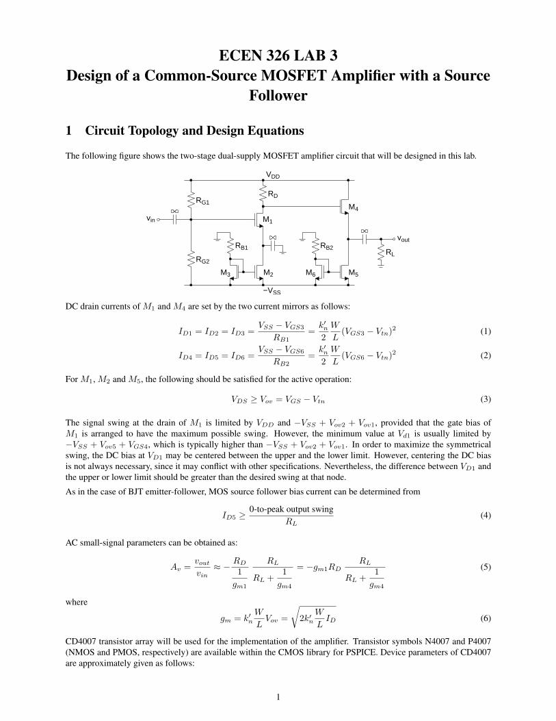
The following figure shows the two-stage dual-supply MOSFET amplifier circuit that will be designed in this lab.
M1
M2
M4
M5
RD
RL
vout
M3
RB1
M6
RB2
RG2
RG1
vin
VDD
−VSS
DC drain currents of M1 and M4 are set by the two current mirrors as follows:
ID1 = ID2 = ID3 =VSS − VGS3
RB1=
k′n
2W
L(VGS3 − Vtn)2 (1)
ID4 = ID5 = ID6 =VSS − VGS6
RB2=
k′n
2W
L(VGS6 − Vtn)2 (2)
For M1, M2 and M5, the following should be satisfied for the active operation:
VDS ≥ Vov = VGS − Vtn (3)
The signal swing at the drain of M1 is limited by VDD and −VSS + Vov2 + Vov1, provided that the gate bias ofM1 is arranged to have the maximum possible swing. However, the minimum value at Vd1 is usually limited by−VSS + Vov5 + VGS4, which is typically higher than −VSS + Vov2 + Vov1. In order to maximize the symmetricalswing, the DC bias at VD1 may be centered between the upper and the lower limit. However, centering the DC biasis not always necessary, since it may conflict with other specifications. Nevertheless, the difference between VD1 andthe upper or lower limit should be greater than the desired swing at that node.
As in the case of BJT emitter-follower, MOS source follower bias current can be determined from
ID5 ≥0-to-peak output swing
RL(4)
AC small-signal parameters can be obtained as:
Av =vout
vin≈ − RD
1gm1
RL
RL +1
gm4
= −gm1RDRL
RL +1
gm4
(5)
where
gm = k′n
W
LVov =
√2k′
n
W
LID (6)
CD4007 transistor array will be used for the implementation of the amplifier. Transistor symbols N4007 and P4007(NMOS and PMOS, respectively) are available within the CMOS library for PSPICE. Device parameters of CD4007are approximately given as follows:
1
NMOS PMOSk′
n = 100 µA/V 2 k′p = 50 µA/V 2
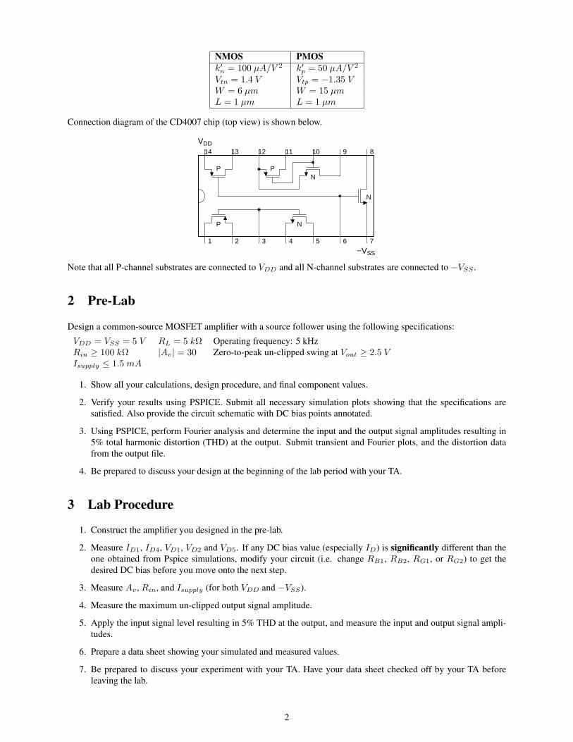
Vtn = 1.4 V Vtp = −1.35 VW = 6 µm W = 15 µmL = 1 µm L = 1 µm
Connection diagram of the CD4007 chip (top view) is shown below.
N
−VSS
VDD
21 3 4 5 6 7
14 13 12 11 10 9 8
PPN
NP
Note that all P-channel substrates are connected to VDD and all N-channel substrates are connected to −VSS .
2 Pre-Lab
Design a common-source MOSFET amplifier with a source follower using the following specifications:
VDD = VSS = 5 V RL = 5 kΩ Operating frequency: 5 kHzRin ≥ 100 kΩ |Av| = 30 Zero-to-peak un-clipped swing at Vout ≥ 2.5 VIsupply ≤ 1.5 mA
1. Show all your calculations, design procedure, and final component values.
2. Verify your results using PSPICE. Submit all necessary simulation plots showing that the specifications aresatisfied. Also provide the circuit schematic with DC bias points annotated.
3. Using PSPICE, perform Fourier analysis and determine the input and the output signal amplitudes resulting in5% total harmonic distortion (THD) at the output. Submit transient and Fourier plots, and the distortion datafrom the output file.
4. Be prepared to discuss your design at the beginning of the lab period with your TA.
3 Lab Procedure
1. Construct the amplifier you designed in the pre-lab.
2. Measure ID1, ID4, VD1, VD2 and VD5. If any DC bias value (especially ID) is significantly different than theone obtained from Pspice simulations, modify your circuit (i.e. change RB1, RB2, RG1, or RG2) to get thedesired DC bias before you move onto the next step.
3. Measure Av , Rin, and Isupply (for both VDD and −VSS).
4. Measure the maximum un-clipped output signal amplitude.
5. Apply the input signal level resulting in 5% THD at the output, and measure the input and output signal ampli-tudes.
6. Prepare a data sheet showing your simulated and measured values.
7. Be prepared to discuss your experiment with your TA. Have your data sheet checked off by your TA beforeleaving the lab.
2

ECEN 326 LAB 4Design of a BJT Differential Amplifier
1 Circuit Topology and Design Equations
The following figure shows a typical BJT differential amplifier. Assume β ≥ 100 and VA = 75 V .
Vo1 Vo2
VCC
−VEE
RC RC
RE RE
RB3 RB2
RB1
Vi1 Vi2
Q1 Q2
Q3
RT IT
The tail current source (IT ) can be calculated from
IT ≈
RB2
RB1 + RB2VEE − 0.7
RB3
provided that IB3 IRB2 . DC collector currents of Q1 and Q2 are
IC1 = IC2 ≈IT
2
Assuming ro1, ro2 RC , RE , small-signal differential-mode gain can be obtained as
Adm =vod
vid≈ − RC
re1 + RE
where re1 ≈ VT /IC1. Common-mode gain can be found as
Acm =voc
vic≈ − RC
re1 + RE + 2RT
where
RT = ro3 + RBB + gm3rπ3
rπ3 + (RB1 ‖ RB2)ro3RBB
RBB = RB3 ‖ (rπ3 + (RB1 ‖ RB2))
Common-mode rejection ratio (CMRR), differential-mode input resistance (Rid) and common-mode input resistance(Ric) are given by
CMRR = 20 log∣∣∣∣Adm
Acm
∣∣∣∣Rid ≈ 2(β + 1)(RE + re1)Ric ≈ (β + 1)(2RT ‖ ro1)
1

Because of mismatches between the transistors and load resistors, a non-zero differential output voltage will resultwhen the differential input voltage is zero. We may refer this output offset voltage back to the input as
VOS =Vo
Adm
VOS is known as the input-referred offset voltage. Since the two sources of the offset voltage are uncorrelated, it canbe estimated as
VOS = VT
√(∆RC
RC
)2
+(
∆IS
IS
)2
2 Pre-Lab
Design a BJT differential amplifier with the following specifications:
Vic = 0 V Isupply ≤ 3 mA Zero-to-peak un-clipped swing at Vo1 ≥ 2.5 VVCC = VEE = 5 V |Adm| = 40 Operating frequency: 1 kHzRid ≥ 20 kΩ CMRR ≥ 70 dB
1. Show all your calculations and final component values.
2. Verify your results using PSPICE. Submit all necessary simulation plots showing that the specifications aresatisfied. Also provide the circuit schematic with DC bias points annotated.
3. Using PSPICE, perform Fourier analysis and determine the differential input and output signal amplitudes re-sulting in 1% and 5% total harmonic distortion (THD) at the differential output. Submit transient and Fourierplots, and the distortion data from the output file for both cases.
4. Be prepared to discuss your design at the beginning of the lab period with your TA.
3 Lab Procedure
1. Construct the amplifier you designed in the pre-lab.
2. Connect Vi1 and Vi2 to ground and record all DC quiescent voltages and currents.
3. Measure Isupply and the output offset voltage Vo1 − Vo2.
4. Using a 1:1 center-tapped transformer, apply differential input signals to the amplifier as shown below:
1:1
Signal
Vi2
Vi1
Generator
5. Measure the maximum un-clipped output signal amplitude at Vo1.
6. Measure Adm and Rid.
7. Apply the input signal levels resulting in 1% and 5% THD at the differential output voltage, and measure theinput and output signal amplitudes.
8. Disconnect the transformer and connect both inputs to the signal generator. Measure Acm and calculate CMRR.
9. Prepare a data sheet showing your simulated and measured values.
10. Be prepared to discuss your experiment with your TA. Have your data sheet checked off by your TA beforeleaving the lab.
2

ECEN 326 LAB 5Design of a MOS Differential Amplifier
1 Circuit Topology
The following figure shows a typical MOS differential amplifier. Assume k′n = 100 µA/V 2, Vtn = 1.4 V , λn =0.01 V −1, W = 6 µm, and L = 1 µm for all NMOS transistors.
Vo1 Vo2
VDD
RD RD
Vi1 Vi2
M1 M2
RTIT
−VSS
RB
M3M4
The tail current source (IT ) can be calculated from
VSS = ID4RB + VGS4
ID4 =k′n2
W
L(VGS4 − Vtn)2
IT = ID3 = ID4
DC drain currents of M1 and M2 are
ID1 = ID2 =IT
2
Assuming ro1, ro2 RD, small-signal differential-mode gain can be obtained as
Adm =vod
vid≈ − RD
1gm1
= −gm1RD
where gm1 =
√2k′n
W
LID1. Common-mode gain can be found as
Acm =voc
vic≈ − RD
1gm1
+ 2RT
where RT = ro3 =1
λnID3. Common-mode rejection ratio (CMRR) can be calculated from
CMRR = 20 log∣∣∣∣Adm
Acm
∣∣∣∣
1

2 Pre-Lab
Design a MOS differential amplifier with the following specifications:
Vic = 0 V Isupply ≤ 0.5 mA THD ≤ 5% for Vod = 5 V 0-to-peak @ 1 kHzVDD = VSS = 5 V |Adm| ≥ 10
1. Show all your calculations, design procedure, and final component values.
2. Simulate your circuit using N4007 transistor models in PSPICE. Submit all necessary simulation plots showingthat the specifications are satisfied. Also provide the circuit schematic with DC bias points annotated.
3. Using PSPICE, perform Fourier analysis and show that the total harmonic distortion (THD) is less than 5%when the differential output voltage (Vod) is 5 V zero-to-peak at 1 kHz. Submit transient and Fourier plots forVod, and the distortion data from the output file.
4. Be prepared to discuss your design at the beginning of the lab period with your TA.
3 Lab Procedure
1. Construct the amplifier you designed in the pre-lab.
2. Connect Vi1 and Vi2 to ground and record all DC quiescent voltages and currents. If any DC bias value (espe-cially ID) is significantly different than the one obtained from Pspice simulations, modify your circuit to getthe desired DC bias before you move onto the next step.
3. Measure Isupply and the output offset voltage Vo1 − Vo2.
4. Using a 1:1 center-tapped transformer, apply differential input signals at 1 kHz to the amplifier as shown below,and measure Adm.
1:1
Signal
Vi2
Vi1
Generator
5. Adjust the input signal level so that the differential output voltage is 5 V zero-to-peak. Measure the THD at thedifferential output.
6. Disconnect the transformer and connect both inputs to the signal generator. Measure Acm and calculate CMRR.
7. Prepare a data sheet showing your simulated and measured values.
8. Be prepared to discuss your experiment with your TA. Have your data sheet checked off by your TA beforeleaving the lab.
N
−VSS
VDD
21 3 4 5 6 7
14 13 12 11 10 9 8
PPN
NP
CD4007
2

ECEN 326 LAB 6Design of Current Mirrors
1 Circuit TopologiesNPN Simple Current Mirror:
Q1
RC
RE1
VCC
Q2
RE2
Vo
Io
RB
Ro
Io ≈VCC − 0.7RC + RE1
RE1
RE2, Vo,min = VCE2,sat + IoRE2
Ro = g′m2ro2R′E + ro2 + R′
E
g′m2 = gm2rπ2
rπ2 + RB, R′
E = RE2 ‖ (rπ2 + RB)
RB = RC ‖ (re1 + RE1)
NPN Simple Current Mirror with β Helper:
1
RC
Q3
RE1
Q2
RE2
VCC
RB
Q
Vo
IoRo
x
Io ≈VCC − 1.4RC + RE1
RE1
RE2, Vo,min = VCE2,sat + IoRE2
Ro = g′m2ro2R′E + ro2 + R′
E
g′m2 = gm2rπ2
rπ2 + RB, R′
E = RE2 ‖ (rπ2 + RB)
RB =(
RC
β + 1+
(β + 1)re1
N
)‖
[re1 + RE1
β
(1 +
(β + 1)2re1
NRC
)]‖ (β + 1)(re1 + RE1)
N : Number of base terminals connected to the node ©x
NMOS Simple Current Mirror:
M1 M2
RC
VCCVo
IoRo
ID1 =VCC − VGS1
RC=
k′n2
(W
L
)1
(VGS1 − Vtn)2 , Vtn < VGS1 < VCC
Io =(W/L)2(W/L)1
ID1 , Vo,min = VGS1 − Vtn = Vov1
Ro = ro2
PMOS Simple Current Mirror:VCC
Vo
Io RoRC
M1 M2ID1 =
VCC − VSG1
RC=
k′p2
(W
L
)1
(VSG1 − |Vtp|)2 , |Vtp| < VSG1 < VCC
Io =(W/L)2(W/L)1
ID1 , Vo,max = VCC − (VSG1 − |Vtp|) = VCC − Vov1
Ro = ro2
NMOS Cascode Current Mirror:
M3 M4
RC
VCCVo
IoRo
M1 M2
−VCC
(W/L)1 = (W/L)3 , (W/L)2 = (W/L)4
ID1 =2VCC − 2VGS1
RC=
k′n2
(W
L
)1
(VGS1 − Vtn)2 , Vtn < VGS1 <VCC
2
Io =(W/L)2(W/L)1
ID1 , Vo,min = −VCC + VGS1 + Vov1 = −VCC + 2Vov1 + Vtn
Ro = gm4ro4ro2 + ro4 + ro2
1

2 Pre-Lab
The following table shows transistor device parameters. Use VCC = 5V for all calculations.
NPN NMOS PMOSQ2N3904 N4007 P4007β = 140 k′n = 100 µA/V 2 k′p = 50 µA/V 2
VCE,sat = 0.2 V Vtn = 1.4 V Vtp = −1.35 VVA = 75 V W = 6 µm W = 15 µm
L = 1 µm L = 1 µmλn = 0.01 V −1 λp = 0.02 V −1
1. Calculate RC , Ro, and the output operating voltage range for the current mirrors in the following table:
(a) NPN Simple Current Mirror RE1 = RE2 = 100Ω Io = 1mA(b) NPN Simple Current Mirror with β Helper RE1 = RE2 = 100Ω Io = 1mA(c) NPN Simple Current Mirror with β Helper RE1 = 100Ω, RE2 = 50Ω, Q2 = 2×Q1
† Io = 2mA(d) NMOS Simple Current Mirror (W/L)1 = (W/L)2 = 6µ/1µ Io = 100µA(e) NMOS Simple Current Mirror (W/L)1 = 6µ/1µ, (W/L)2 = 12µ/1µ Io = 200µA(f) PMOS Simple Current Mirror (W/L)1 = (W/L)2 = 15µ/1µ Io = 100µA(g) NMOS Cascode Current Mirror W/L = 6µ/1µ Io = 100µA
†Q2 is composed of two transistors (each identical to Q1) connected in parallel.
2. For each current mirror, perform DC simulation by sweeping Vo from 0 to VCC (for the cascode mirror, from−VCC to VCC), and plot the output current Io.
3. For each current mirror, perform AC simulation while Vo,dc = 2V , and plot the output resistance Ro.
4. Submit all simulation plots and the circuit schematics with DC bias points annotated (@ Vo = 2V ).
5. Be prepared to discuss your designs at the beginning of the lab period with your TA.
3 Lab Procedure
1. Construct all current mirrors you designed in the pre-lab.
2. For each circuit, measure Io, Ro and the output operating voltage range.
3. Prepare a data sheet showing your simulated and measured values.
4. Be prepared to discuss your experiment with your TA. Have your data sheet checked off by your TA beforeleaving the lab.
2

ECEN 326 LAB 7Design of a BJT Operational Transconductance Amplifier
1 Circuit Topology
The operational transconductance amplifier (OTA) schematic that will be designed in this lab is shown in Fig. 1.
E1
−VEE
RB3 RB2
RB1
VCC
RE3
RL
Q1 Q2
Q4Q3
Q9
Q8
Q6Q5
Q7
R
VoIo
RE2RE2RE3
RE4 RE4
RE1
vid
2
vid
2
IT
VB1 VB2
Matching transistors:Q1 = Q2
Q3 = Q4
Q5 = Q6
Q7 = Q8
NPN PNPQ2N3904 Q2N3906
β 140 180VA 75 V 20 V
Figure 1: Operational transconductance amplifier (OTA) schematic.
DC Biasing and Large-Signal Analysis:Assuming IB9 IRB2 , the tail current source (IT ) can be calculated from
IT ≈
RB2
RB1 + RB2VEE − 0.7
RB3(1)
Collector currents of Q1 −Q4 for Vid = 0 can be found as
IC1−C4 ≈IT
2(2)
If the ratio of I5 to I3 is less than an order of magnitude, then VEB5 ≈ VEB3, therefore,
IC5RE3 = IC3RE2 ⇒ IC5
IC3≈ RE2
RE3(3)
An OTA is commonly used in the open-loop configuration. For proper operation, the maximum differential inputamplitude |vid,max| needs to be determined. With emitter degeneration resistors RE1, |vid,max| can be approximatelyfound as
|vid,max| = IT RE1 (4)
1

A more accurate limit can be defined by a maximum distortion specification. It is also necessary to determine whatrange of common-mode input voltages will allow all transistors in the input stage to remain in the active region. Defin-ing the minimum collector-emitter voltage for the active operation as VCE,sat, the range of VCM can be approximatelygiven by
VCC − IT RE2 − VCE,sat > VCM > −VEE + IT RB3 + VCE,sat + IT RE1 + VBE,on (5)
AC Small-Signal Analysis:Since the circuit is not symmetrical, half-circuit concepts will not be useful. Figure 2 shows the AC small-signalequivalent circuit to determine the equivalent transconductance
Gm =−isc
vid(6)
where the output resistances (ro) of transistors are assumed to be infinite.
e5
ic5
re5
RE3
ic3
re3
RE2 RE2
re4
RE3
re6ie6
ic4
ie1 re1
RT
vid
2
vid
2re2 ie2
RE4
re7
RE4
re8 ie8
ic6
ic8
isc
RE1 RE1vx
ie6αie5α
ie2αie1α
ie8α
i
Figure 2: Small-signal circuit of the OTA.
KCL at vx yields
vx
RT+
vx −(−vid
2
)re1 + RE1
+vx −
(vid
2
)re2 + RE1
= 0 (7)
Since Q1 and Q2 are identical, re1 = re2, resulting in
vx
RT+
vx
re1 + RE1+
vx
re2 + RE1= 0 ⇒ vx = 0 (8)
Therefore, vx is a virtual AC ground for differential input signals. The collector current of Q6 can be found as follows:
ic4 = αie2 ≈vid/2
RE1 + re2(9)
ic6 ≈ic4(RE2 + re4)
RE3 + re6=
vid
21
RE1 + re2
RE2 + re4
RE3 + re6(10)
2

Similarly, ic5 and ic8 can be found as
ic5 ≈ −vid
21
RE1 + re1
RE2 + re3
RE3 + re5(11)
ic8 ≈ ic5RE4 + re7
RE4 + re8(12)
Since Q7 and Q8 are identical, re7 = re8, which yields
ic8 ≈ −vid
21
RE1 + re1
RE2 + re3
RE3 + re5(13)
The short-circuit output current (isc) can be determined as
isc = ic6 − ic8 =vid
21
RE1 + re2
RE2 + re4
RE3 + re6−
(−vid
21
RE1 + re1
RE2 + re3
RE3 + re5
)(14)
Using the matching data, re2 = re1, re4 = re3, re6 = re5,
isc = vid1
RE1 + re2
RE2 + re4
RE3 + re6(15)
(16)
Gm = − 1RE1 + re2
RE2 + re4
RE3 + re6(17)
The differential input resistance can be found as
Rid = 2(β + 1)(re2 + RE1)
The output resistance can be expressed as
Ro ≈ (g′m6ro6R′E3 + ro6) ‖ (g′m8ro8R
′E4 + ro8) (18)
g′m6 = gm6rπ6
rπ6 + re4 + RE2, R′
E3 = RE3 ‖ (rπ6 + re4 + RE2) (19)
g′m8 = gm8rπ8
rπ8 + re7 + RE4, R′
E4 = RE4 ‖ (rπ8 + re7 + RE4) (20)
We may construct an equivalent small-signal model for the OTA as shown in Fig. 3.
GmvidRid Rovid
RL
io
Figure 3: Equivalent small-signal model of the OTA.
2 Pre-Lab
Design an OTA with the following specifications:
VCC = VEE = 5 V Gm = 1mA/V Operating frequency: 1 kHz|vid,max| ≥ 2V VCM,max − VCM,min ≥ 4V Isupply ≤ 5mA
1. Show all your calculations and final component values.
3

2. Calculate Rid and Ro for your design.
3. Verify your results using PSPICE (use Q2N3904 and Q2N3906 transistors). Submit all necessary simulationplots showing that the specifications are satisfied. Also provide the circuit schematic with DC bias pointsannotated.
4. Be prepared to discuss your design at the beginning of the lab period with your TA.
3 Lab Procedure
1. Construct the OTA you designed in the pre-lab.
2. Set Vid = 0 and record all DC quiescent voltages and currents.
3. Measure Isupply and the short-circuit output current while Vid = 0.
4. Using a 1:1 center-tapped transformer, apply differential input signals to the amplifier as shown below:
1:1
Signal
VB2
VB1
Generator
5. Connect a 1kΩ resistor between the output node and ground. Using the XY mode of the scope, monitor Vo vs.VB1. Measure the slope and calculate the resulting Gm.
6. Increase the input amplitude until nonlinearity occurs. Measure and record the width of the input linear range(|vid,max|).
7. Disconnect the transformer, ground VB2 and the output node, and measure the differential input resistance Rid
at VB1.
8. Using the circuit setup below, measure and record the transconductance (Gm) of your OTA.1k
GmVB2
VB1
100µ
R1
Vo
Vs
Vo
Vs=
1/Gm
R1 + (1/Gm)
9. Connect the OTA as shown in the figure below and set the amplitude of Vs to |vid,max|. Using the XY mode ofthe scope, monitor Vo vs. Vs. Vary the potentiometer in both directions until nonlinearity occurs. Measure andrecord the DC voltage at VB2 at the two settings of the potentiometer where distortion occurs. Record these twomeasurements as VCM,max and VCM,min.
1k
Gm
−VEEVCC
10k
VB1
VB2
R1
100µ
100µ
Vo
VsVo
Vs=
1/Gm
R1 + (1/Gm)
10. Prepare a data sheet showing your simulated and measured values.
11. Be prepared to discuss your experiment with your TA. Have your data sheet checked off by your TA beforeleaving the lab.
4

ECEN 326 LAB 8Frequency Response of a Common-Emitter BJT Amplifier
1 Circuit Topology
Circuit schematic of the common-emitter amplifier is shown in Fig. 1. Capacitors CB and CC are used for ACcoupling, whereas CE is an AC bypass capacitor used to establish an AC ground at the emitter of Q1. CF is a smallcapacitance that will be used to control the higher 3-dB frequency of the amplifier.
RS
RB2
RB1
Vs
CF
CB
VCC
Q1
RC
RE
RL
CE
CC
Vo
Rin
Rout
Figure 1: Common-emitter BJT amplifier.
1.1 DC Biasing and Mid-band Frequency Response
For this section, assume that CB = CC = CE =∞ and CF = Cπ = Cµ = 0. You can find the DC collector current(IC) and the resistor values following the analysis provided in Lab #1. Since the topology and the requirements areslightly different, you need to make minor modifications to the design procedure and equations.
1.2 Low Frequency Response
Figure 2 shows the low-frequency small-signal equivalent circuit of the amplifier. Note that CF is ignored since itsimpedance at these frequencies is very high.
RS CB
RB rπ vπ vπgmvs
RECE
CC
RC RL
vo
Figure 2: Low-frequency equivalent circuit.
Using short-circuit time constant analysis, the lower 3-dB frequency (ωL) can be found as
ωL ≈1
R1sCB+
1R2sCE
+1
R3sCC(1)
where
R1s = RS + (RB ‖ rπ) (2)
R2s = RE ‖(
rπ + (RB ‖ RS)β + 1
)(3)
R3s = RC + RL (4)
1

1.3 High Frequency Response
At high frequencies, CB , CC and CE can be replaced with a short circuit since their impedances become very small.Figure 3 shows the high-frequency small-signal equivalent circuit of the amplifier.
F
RBvs
RS rb
rπ vπ vπgm RC RL
vo
Cπ
Cµ +C
Figure 3: High-frequency equivalent circuit.
The higher 3-dB frequency (ωH ) can be derived as
ωH =1
RT
[Cπ + (Cµ + CF )
(1 + gmRCL +
RCL
RT
)] (5)
where
RT = rπ ‖ (rb + (RS ‖ RB)) (6)RCL = RC ‖ RL (7)
Thus, if we assume that the common-emitter amplifier is properly characterized by these dominant low and highfrequency poles, then the frequency response of the amplifier can be approximated by
vo
vs(s) = Av
s
s + ωL
1
1 +s
ωH
(8)
2 Pre-Lab
Assuming CB = CC = CE = ∞ and CF = Cπ = Cµ = 0, and using a Q2N2222 BJT, design a common-emitteramplifier with the following specifications:
VCC = 5 V RS = 50Ω RL = 1 kΩRin ≥ 250 Ω Isupply ≤ 8mA |Av| ≥ 50 0-to-peak unclipped output swing ≥ 1.5 V
1. Show all your calculations, design procedure, and final component values.
2. Verify your results using PSPICE. Submit all necessary simulation plots showing that the specifications aresatisfied. Also provide the circuit schematic with DC bias points annotated.
3. Using PSPICE, find the higher 3-dB frequency (fH) while CF = 0.
4. Determine Cπ , Cµ and rb of the transistor from the PSPICE output file (in Probe, choose View → Output File,scroll down to the section OPERATING POINT INFORMATION, Cπ , Cµ and rb are listed as CBE, CBC andRX, respectively). Calculate fH using Eq. (5) and compare it with the simulation result obtained in Step 3.
5. Calculate the value of CF to have fH = 20 kHz. Simulate the circuit to verify your result, and adjust the valueof CF if necessary.
6. Calculate CB , CC , CE to have fL = 500 Hz. Simulate the circuit to verify your result, and adjust the values ofcapacitors if necessary.
7. Be prepared to discuss your design at the beginning of the lab period with your TA.
2

3 Lab Procedure
1. Construct the amplifier you designed in the pre-lab.
2. Measure IC , VE , VC and VB . If any DC bias value is significantly different than the one obtained from Pspicesimulations, modify your circuit to get the desired DC bias before you move onto the next step.
3. Measure Isupply .
4. Obtain the magnitude of the frequency response of the amplifier and determine the lower and higher 3-dBfrequencies fL and fH .
5. At midband frequencies, measure Av , Rin, and Rout.
6. Measure the maximum un-clipped output signal amplitude.
7. Prepare a data sheet showing your simulated and measured values.
8. Be prepared to discuss your experiment with your TA. Have your data sheet checked off by your TA beforeleaving the lab.
3

ECEN 326 LAB 9Frequency Response of a Cascode BJT Amplifier
1 Circuit Topology
Circuit schematic of the cascode amplifier is shown in Fig. 1. Capacitors CB and CC are used for AC coupling,whereas CD and CE are AC bypass capacitors. CF is a small capacitance that will be used to control the higher 3-dBfrequency of the amplifier.
Vs
CB
RE CERin
RB2
RB1
VCC CF
Q1
Q2
RC
VCC
RLCC
Vo
Rout
RS
CDRB4
RB3
Figure 1: Cascode BJT amplifier.
1.1 DC Biasing and Mid-band Frequency Response
For this section, assume that CB = CC = CD = CE =∞ and CF = Cπ = Cµ = 0. You can find the DC collectorcurrents (IC1 and IC2) and the resistor values following the analysis provided in Lab #2. Since the topology and therequirements are slightly different, you need to make minor modifications to the design procedure and equations.
1.2 Low Frequency Response
Using short-circuit time constant analysis, the lower 3-dB frequency (ωL) can be found as
ωL ≈1
R1sCB+
1R2sCE
+1
R3sCD+
1R4sCC
(1)
where
R1s = RS + (RB1 ‖ RB2 ‖ rπ1) (2)
R2s = RE ‖(
re1 +RB1 ‖ RB2 ‖ RS
β + 1
)(3)
R3s = RB3 ‖ RB4 (4)R4s = RC + RL (5)
1

1.3 High Frequency Response
The higher 3-dB frequency (ωH ) can be estimated using open-circuit time constant analysis
ωH ≈ 1R1oCπ1 + R2o(Cµ1 + CF ) + R3oCπ2 + R4oCµ2
(6)
where
R1o = rπ1 ‖ (rb1 + (RB1 ‖ RB2 ‖ RS)) (7)R2o = R1o + re2 + gm1R1ore2 (8)
R3o = rπ2 ‖1
gm2(9)
R4o = RC ‖ RL (10)
Thus, if we assume that the cascode amplifier is properly characterized by these dominant low and high frequencypoles, then the frequency response of the amplifier can be approximated by
vo
vs(s) = Av
s
s + ωL
1
1 +s
ωH
2 Pre-Lab
Assuming CB =CC =CD =CE =∞ and CF =Cπ =Cµ =0, and using Q2N2222 BJTs, design a cascode amplifierwith the following specifications:
VCC = 5 V RS = 50Ω RL = 1 kΩRin ≥ 250 Ω Isupply ≤ 8mA |Av| ≥ 50 0-to-peak unclipped output swing ≥ 1.5 V
1. Show all your calculations, design procedure, and final component values.
2. Verify your results using PSPICE. Submit all necessary simulation plots showing that the specifications aresatisfied. Also provide the circuit schematic with DC bias points annotated.
3. Using PSPICE, find the higher 3-dB frequency (fH) while CF = 0.
4. Determine Cπ , Cµ and rb for both transistors from the PSPICE output file (in Probe, choose View → OutputFile, scroll down to the section OPERATING POINT INFORMATION, Cπ , Cµ and rb are listed as CBE, CBCand RX, respectively). Calculate fH using Eq. (6) and compare it with the simulation result obtained in Step 3.
5. Calculate the value of CF to have fH = 20 kHz. Simulate the circuit to verify your result, and adjust the valueof CF if necessary.
6. Calculate CB , CC , CD and CE to have fL = 500 Hz. Simulate the circuit to verify your result, and adjust thevalues of capacitors if necessary.
7. Compare the value of fH for CF = 0 with that of the common-emitter amplifier designed in the previous lab.Also compare the values of CF required to obtain fH = 20 kHz. Comment on the differences.
8. Be prepared to discuss your design at the beginning of the lab period with your TA.
2

3 Lab Procedure
1. Construct the amplifier you designed in the pre-lab.
2. Measure IC , VC , VB and VE for both transistors. If any DC bias value is significantly different than the oneobtained from Pspice simulations, modify your circuit to get the desired DC bias before you move onto the nextstep.
3. Measure Isupply .
4. Obtain the magnitude of the frequency response of the amplifier and determine the lower and higher 3-dBfrequencies fL and fH .
5. At midband frequencies, measure Av , Rin, and Rout.
6. Measure the maximum un-clipped output signal amplitude.
7. Prepare a data sheet showing your simulated and measured values.
8. Be prepared to discuss your experiment with your TA. Have your data sheet checked off by your TA beforeleaving the lab.
3
ECEN 326 LAB 10Design of a BJT Shunt-Series Feedback Amplifier
1 Circuit Topology
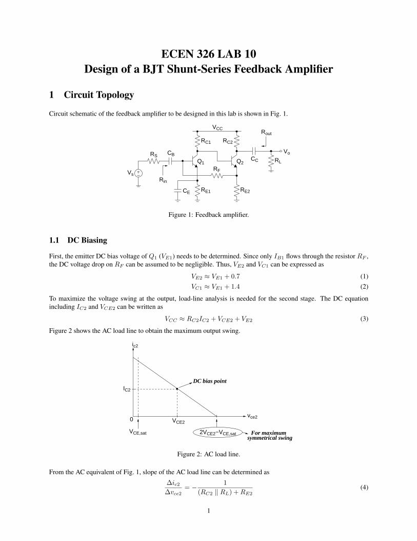
Circuit schematic of the feedback amplifier to be designed in this lab is shown in Fig. 1.
RS
Vs
CB
Rin
RE1CE
VCC
Q2 RLCC
Vo
Rout
RF
RC1
Q1
RE2
RC2
Figure 1: Feedback amplifier.
1.1 DC Biasing
First, the emitter DC bias voltage of Q1 (VE1) needs to be determined. Since only IB1 flows through the resistor RF ,the DC voltage drop on RF can be assumed to be negligible. Thus, VE2 and VC1 can be expressed as
VE2 ≈ VE1 + 0.7 (1)VC1 ≈ VE1 + 1.4 (2)
To maximize the voltage swing at the output, load-line analysis is needed for the second stage. The DC equationincluding IC2 and VCE2 can be written as
VCC ≈ RC2IC2 + VCE2 + VE2 (3)
Figure 2 shows the AC load line to obtain the maximum output swing.
symmetrical swing
c2
VCE,sat
vce2
DC bias point
−VCE,sat
VCE2
IC2
2VCE2
0
For maximum
i
Figure 2: AC load line.
From the AC equivalent of Fig. 1, slope of the AC load line can be determined as
∆ic2∆vce2
= − 1(RC2 ‖ RL) + RE2
(4)
1

Using the slope and the DC bias point (ic2, vce2) = (IC2, VCE2), the load line equation can be obtained as
ic2 − IC2
vce2 − VCE2= − 1
(RC2 ‖ RL) + RE2(5)
Evaluating Eq. (5) at the point (ic2, vce2) = (0, 2VCE2 − VCE,sat),
IC2((RC2 ‖ RL) + RE2) = VCE2 − VCE,sat (6)
Solving Eqs. (3) and (6), the optimum IC2 to obtain the maximum symmetrical swing can be found as
IC2 =VCC − 2VE2 − VCE,sat
RC2 + (RC2 ‖ RL)(7)
After determining IC2, 0-to-peak voltage swing at the output can be calculated as
Vsw = IC2(RC2 ‖ RL) =VCC − 2VE2 − VCE,sat
1 +RC2
RC2 ‖ RL
=VCC − 2VE2 − VCE,sat
2 +RC2
RL
(8)
Since VE1 and VC1 are already determined, IC1 can be chosen based on other specifications. The remaining compo-nents can be calculated as
RE1 =VE1
IC1(9)
RC1 =VCC − VC1
IC1(10)
RE2 =VE2
IC2(11)
1.2 Feedback Analysis and Mid-band Frequency Response
AC equivalent of the amplifier in the mid-band frequency range is shown in Fig. 3.
Feedback
Q1 RC1
Q2
RE2
RF
RC2RL
ifb
iεiiRS
vs
vo
io
io
network
Figure 3: AC equivalent circuit.
The input port of the feedback network in Fig. 3 is not directly connected to the output node (vo). Therefore, thesampled output signal is not a voltage. Defining the output current as
io = − vo
RL ‖ RC2(12)
it can be concluded that io is sampled by the feedback network. At the amplifier’s input, subtraction of the feedbacksignal is performed in the current domain,
ii − ifb = iε (13)
2

Therefore, the type of feedback is shunt-series. The next step is to obtain the g parameters of the feedback network asshown in Fig. 4.
12f
i1 i2
v1 v2g21f v1
g22f
i2gg11f
1
i1
v1
i2
v2RE2
RF
g11f =i1v1
∣∣∣∣i2=0
=1
RF + RE2
g22f =v2
i2
∣∣∣∣v1=0
= RE2 ‖ RF
g12f =i1i2
∣∣∣∣v1=0
= − RE2
RE2 + RF
Figure 4: Calculation of the g-parameters of the feedback network.
Replacing the feedback network with its two-port equivalent and converting the input source into current, the amplifiercircuit can be arranged as in Fig. 5.
Q1 RC1
Q2
f io io
networkFeedback
RS RF+RE2 RF ||RE2
io
iε vε||RC2RL
vo
vb2
Ri2
=isRS
vs
Figure 5: Amplifier with the ideal feedback network.
From Fig. 5, assuming ro1 and ro2 are large, the parameters a and f can be obtained as follows
vε = iε(RS ‖ (RF + RE2) ‖ rπ1) (14)vb2
vε= −RC1 ‖ Ri2
re1(15)
Ri2 = (β + 1)(re2 + (RF ‖ RE2)) (16)vo
vb2= − RL ‖ RC2
re2 + (RF ‖ RE2)(17)
vo = −io(RL ‖ RC2) (18)
a =ioiε
= − (RS ‖ (RF + RE2) ‖ rπ1)(RC1 ‖ Ri2)re1(re2 + (RF ‖ RE2))
(19)
f = g12f = − RE2
RE2 + RF(20)
The current-mode close-loop amplifier parameters are
Ai =iois
=a
1 + af(21)
Zi =zi
1 + af(22)
Zo = (1 + af)zo (23)
3

where
zi = RS ‖ (RF + RE2) ‖ rπ1 (24)
zo = RT + ro2 + gm2rπ2
rπ2 + (ro1 ‖ RC1)ro2RT (25)
RT = RF ‖ RE2 ‖ [rπ2 + (ro1 ‖ RC1)] (26)
Figure 6 shows the current-mode equivalent model of the amplifier.
is Zi Ai is Zo RC2 RL
io
Figure 6: Current-mode equivalent model of the amplifier.
As the final step, the current-mode model needs to be converted to a voltage-mode amplifier. Figure 7 shows theequivalent amplifier where RS is separated from Zi and the controlled source depends on iin.
is
iin
RS Rin Axiin Zo RC2
io
RL
Rout
Figure 7: Current-mode amplifier with RS separated.
Rin and Ax in Fig. 7 can be found as follows
Zi = RS ‖ Rin =1
1RS
+1
Rin
⇒ Rin =1
1Zi− 1
RS
(27)
iin =RS
RS + Rinis ⇒ Ax = Ai
(1 +
Rin
RS
)(28)
Voltage-mode equivalent model of the amplifier can be obtained after final conversion as shown in Fig. 8.
Rinvs
RS
Av vinvin RL
Routvo
Figure 8: Voltage-mode equivalent model of the amplifier.
Rout and Av in Fig. 8 can be found as follows
Rout = Zo ‖ RC2 ≈ RC2 (29)
Av = −AxRout
Rin= −Ai
(1 +
Rin
RS
)Rout
Rin(30)
Finally, the voltage gain vo/vs can be calculated as
vo
vs=
Rin
RS + RinAv
RL
Rout + RL(31)
4

2 Pre-Lab
Using Q2N2222 transistors, design the feedback amplifier with the following specifications:
VCC = 10 V RS = 50Ω RL = 10 kΩ VE1 ≥ 0.4 Vaf ≥ 5 Isupply ≤ 10mA |vo/vs| ≥ 80 0-to-peak unclipped output swing ≥ 3.5 V
1. Show all your calculations, design procedure, and final component values.
2. Using PSPICE, find a, f , Isupply , Rin, Rout and vo/vs to verify your results. Submit all necessary simulationplots showing that the specifications are satisfied. Also provide the circuit schematic with DC bias pointsannotated.
3. Using PSPICE, perform Fourier analysis to determine the THD of 3.5 V (0-to-peak) output waveform at 1 kHz.Submit transient and Fourier plots, and the distortion data from the output file.
4. Be prepared to discuss your design at the beginning of the lab period with your TA.
3 Lab Procedure
1. Construct the amplifier you designed in the pre-lab.
2. Measure IC , VC , VB and VE for both transistors. If any DC bias value is significantly different than the oneobtained from Pspice simulations, modify your circuit to get the desired DC bias before you move onto the nextstep.
3. Measure Isupply .
4. At midband frequencies, measure vo/vs, Rin and Rout.
5. Measure the maximum un-clipped output signal amplitude.
6. Measure the THD when the output is 3.5 V (0-to-peak) sinewave at 1 kHz.
7. Prepare a data sheet showing your simulated and measured values.
8. Be prepared to discuss your experiment with your TA. Have your data sheet checked off by your TA beforeleaving the lab.
5

ECEN 326 LAB 11Design of a Two-Stage Amplifier with Miller Compensation
1 Circuit Topology
Figure 1 shows the two-stage differential amplifier to be designed in this lab. CL represents the load capacitor, whereasCM is the Miller compensation capacitor.
−VEE
VCC
Vi+Vi− Q1 Q2
Q7
Q6
Q4Q3
RB1
RB2RE2 RE3
RE1
CMRE1
VoCL
Q5
Figure 1: Two-stage differential amplifier.
Defining Vi = (Vi+ − Vi−), the transfer function can be obtained as
Vo
Vi(s) = a(s) ≈ ao(
1− s
p1
) (1− s
p2
) (1)
where
a0 ≈ g′m2Ro1gm7Ro2 (2)
g′m2 ≈gm2
1 + gm2RE1(3)
Ro1 ≈ rπ7 ‖ ro4 ‖ (ro2 + gm2ro2RE1) (4)Ro2 ≈ ro7 ‖ (gm6ro6(RE3 ‖ rπ6) + ro6) (5)
p1 ≈ − 1gm7Ro1Ro2CM
(6)
p2 ≈ −gm7
CL(7)
Assuming |p2| |p1| and |p2| > ωt the unity-gain frequency ωt can be calculated as
ωt = a0|p1| =g′m2
CM(8)
The phase margin for unity-gain configuration (f = 1) is approximately equal to
PM ≈ tan−1
(|p2|ωt
)= tan−1
(gm7
g′m2
CM
CL
)(9)
1

2 Pre-Lab
Using Q2N3904 and Q2N3906 transistors, and assuming βnpn = 140, βpnp = 180, VA,npn = 75 V , VA,pnp = 20 V ,design the two-stage amplifier circuit with the following specifications:
VCC = VEE = 5 V CL = 10 nFRE1 = 200 Ω ao ≥ 80 dB
1. Show all your calculations and final component values.
2. Find a set of CM values which results in PM = 30, 45 and 60.
3. Verify your results using PSPICE. Submit all necessary simulation plots showing that the specifications aresatisfied. Also provide the circuit schematic with DC bias points annotated.
4. Perform AC simulation on the closed-loop circuit in unity-gain configuration for PM = 30, 45 and 60.
5. Apply a 1-V step input and perform transient simulation to obtain the step response for PM = 30, 45 and 60.
6. Submit all simulation plots showing AC and step responses.
7. Be prepared to discuss your design with your TA at the beginning of the lab.
3 Lab Procedure
1. Construct the amplifier you designed in the pre-lab.
2. Measure Isupply and all DC quiescent voltages and currents.
3. Observe the frequency and step responses for PM = 30, 45 and 60.
4. Prepare a data sheet showing your simulated and measured values.
5. Be prepared to discuss your experiment with your TA. Have your data sheet checked off by your TA beforeleaving the lab.
2