ECE 510 Lecture 7 Confidence Intervals -...

ECE 510 Lecture 7 Goodness of Fit, Maximum Likelihood

Scott Johnson

Glenn Shirley

Confidence Limits

30 Jan 2013 ECE 510 S.C.Johnson, C.G.Shirley 2

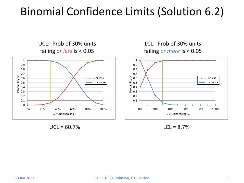
Binomial Confidence Limits (Solution 6.2)


UCL: Prob of 30% units failing or less is < 0.05

LCL: Prob of 30% units failing or more is < 0.05

UCL = 60.7% LCL = 8.7%

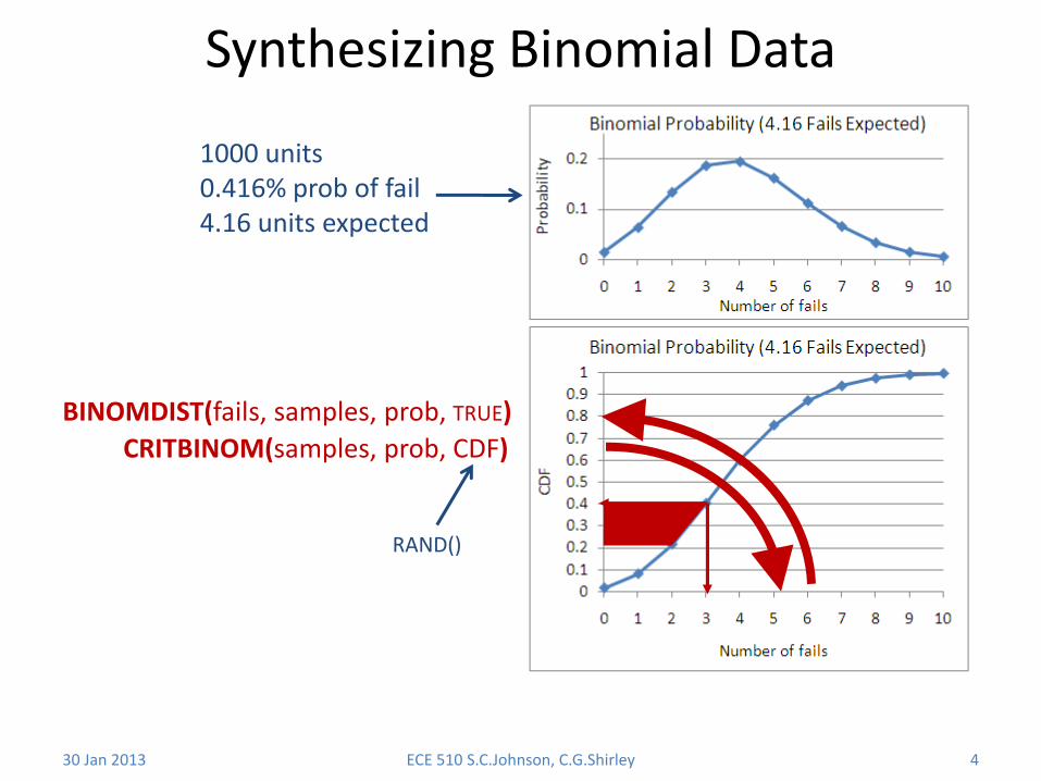
Synthesizing Binomial Data


1000 units 0.416% prob of fail 4.16 units expected

BINOMDIST(fails, samples, prob, TRUE)

CRITBINOM(samples, prob, CDF)

RAND()


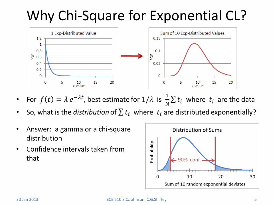
Why Chi-Square for Exponential CL?

• Answer: a gamma or a chi-square distribution

• Confidence intervals taken from that

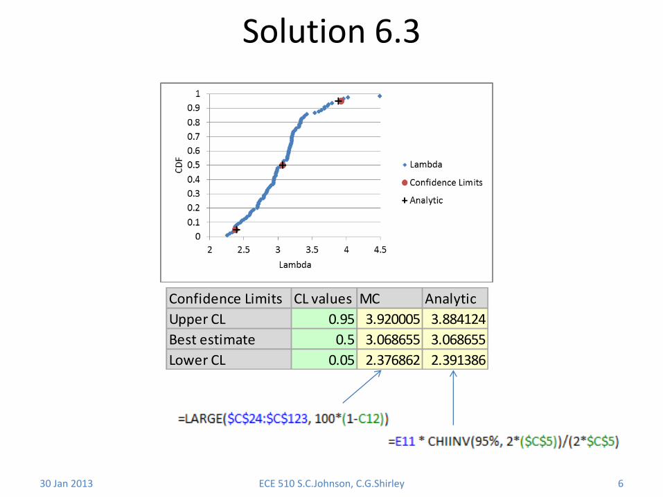
Solution 6.3


Confidence Limits CL values MC Analytic

Upper CL 0.95 3.920005 3.884124

Best estimate 0.5 3.068655 3.068655

Lower CL 0.05 2.376862 2.391386

Confidence Limits Summary • Confidence limits (UCL and LCL) are values between which (2-sided) or

above or below which (1-sided) the true population value falls with <confidence level> probability

– Units are whatever units your data uses

• Confidence level is the probability that the true value lies between (or above or below) your confidence limit(s).

• “CL” can mean either confidence limit or confidence level

– Use context to decide

• Confidence limits can be calculated

– Analytically (best if available)

– Monte Carlo (will work for any distribution)

– Likelihood methods (coming soon)

• Monte Carlo confidence limits work regardless of how you calculate the best estimate


Goodness of Fit Tests


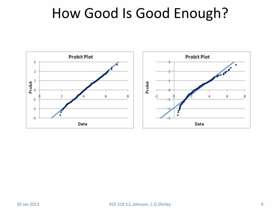
How Good Is Good Enough?


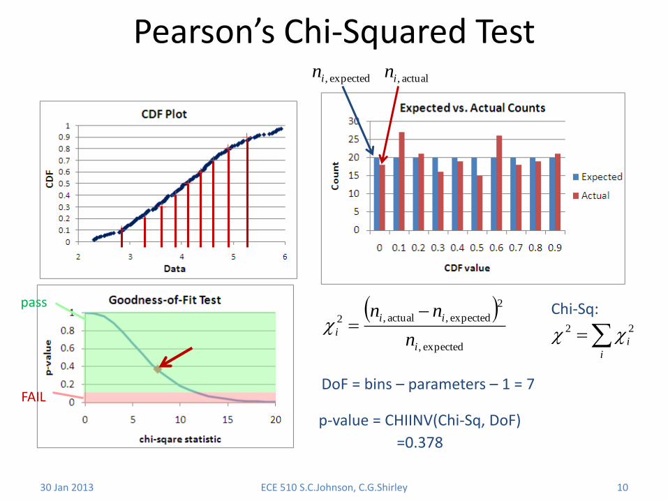
Pearson’s Chi-Squared Test


expected ,

2

expected ,actual ,2

i

ii

in

nn

actual ,inexpected ,in

p-value = CHIINV(Chi-Sq, DoF)

i

i

22

Chi-Sq:

DoF = bins – parameters – 1 = 7

pass

FAIL

=0.378

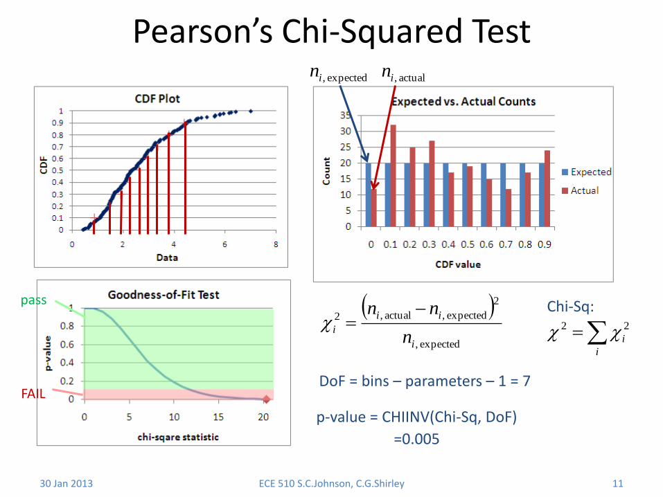
Pearson’s Chi-Squared Test


expected ,

2

expected ,actual ,2

i

ii

in

nn

actual ,inexpected ,in

i

i

22

p-value = CHIINV(Chi-Sq, DoF)

Chi-Sq:

DoF = bins – parameters – 1 = 7

pass

FAIL

=0.005

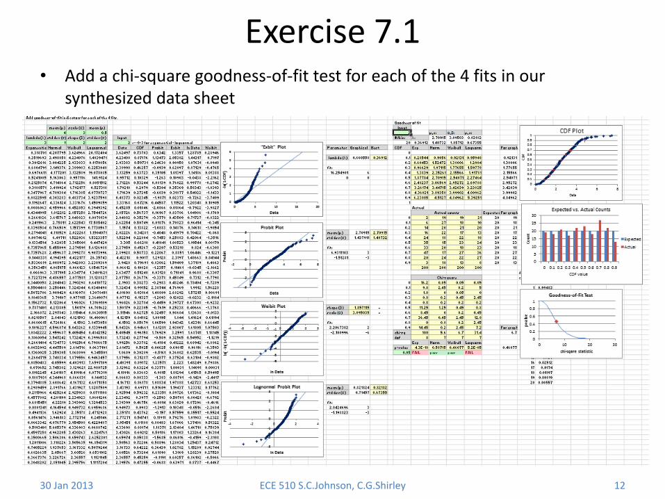
Exercise 7.1


• Add a chi-square goodness-of-fit test for each of the 4 fits in our synthesized data sheet

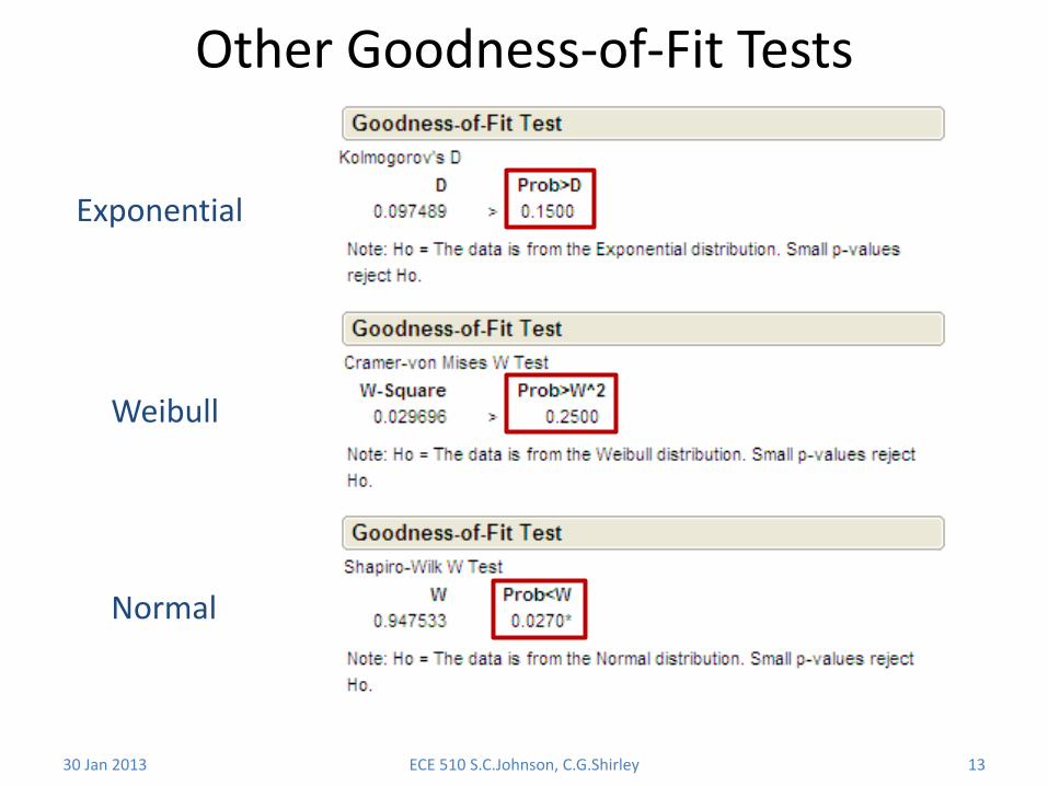
Other Goodness-of-Fit Tests


Exponential

Weibull

Normal

Maximum Likelihood Method and the

Exponential Distribution


MLE • Maximum Likelihood Estimation (MLE) is a fitting technique

that is good for any model

• Principle – We can’t ask: What is the most likely model?

• Because we don’t have some well-defined space of possible models

– We can ask: Given this model, how likely is this data set?

– (This is a fairly Bayesian approach. We are usually frequentists.)


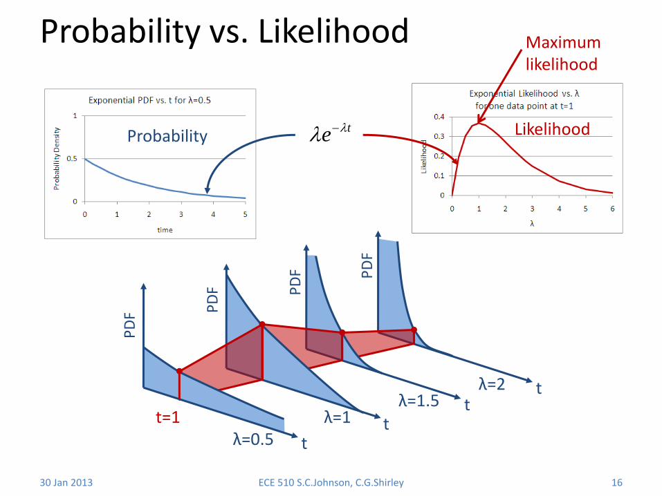
Probability vs. Likelihood


Likelihood

λ=2 t P

DF

λ=1.5 t

PD

F

λ=1 t

PD

F

λ=0.5 t

PD

F Probability

te

Maximum likelihood

t=1

MLE • Likelihood for each point

– For exact values (exact times to fail), use the PDF

– For ranges (failed between two readout times), use CDF delta

– Multiply all together (or add logs)

• Use – Choose a model functional form with adjustable parameters

– Adjust the parameters to maximize the likelihood


MLE for Exponential Data


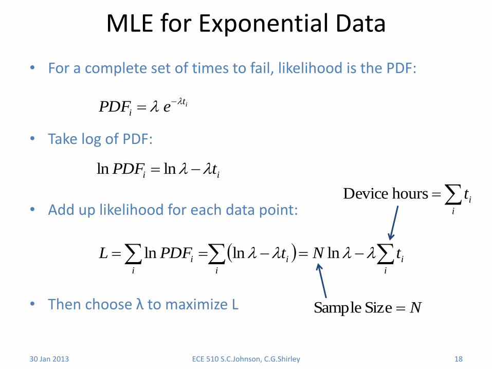
• For a complete set of times to fail, likelihood is the PDF:

• Take log of PDF:

• Add up likelihood for each data point:

• Then choose λ to maximize L

it

i ePDF

ii tPDF lnln

i

i

i

i

i

i tNtPDFL lnlnln

NSize Sample

i

ithours Device

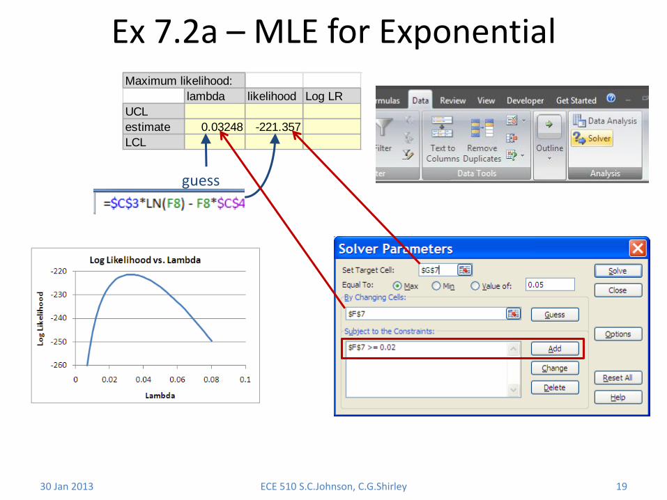
Maximum likelihood:

lambda likelihood Log LR

UCL

estimate 0.03248 -221.357

LCL

Ex 7.2a – MLE for Exponential


guess

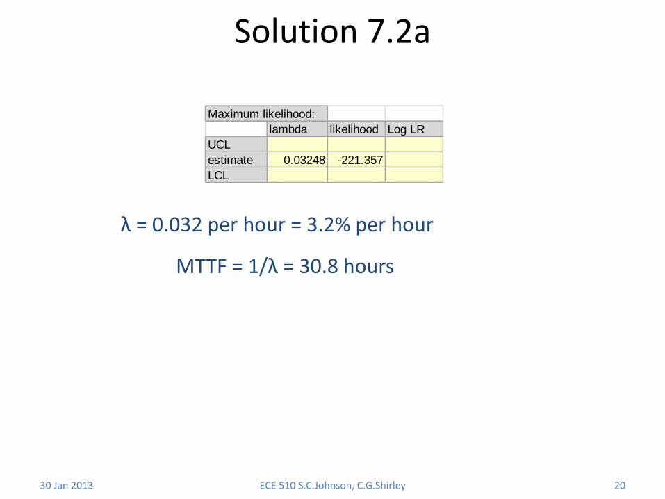
Solution 7.2a


MTTF = 1/λ = 30.8 hours

λ = 0.032 per hour = 3.2% per hour

Maximum likelihood:


UCL

estimate 0.03248 -221.357

LCL

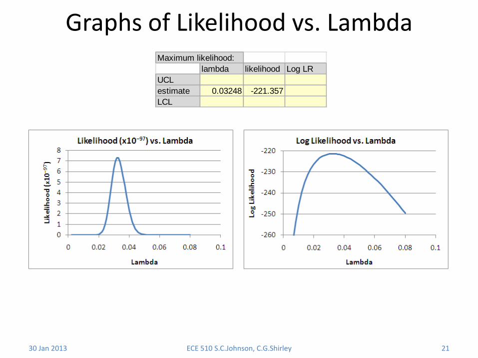
Graphs of Likelihood vs. Lambda


Maximum likelihood:


UCL

estimate 0.03248 -221.357

LCL

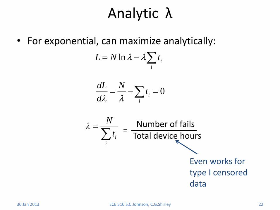
Analytic λ


i

itNL ln

0 i

itN

d

dL

i

it

N =

Number of fails

Total device hours

• For exponential, can maximize analytically:

Even works for type I censored data

Exercise 7.2b

• Calculate λ for the Ex12 data set using the analytic expression and compare it to what you got from the MLE technique


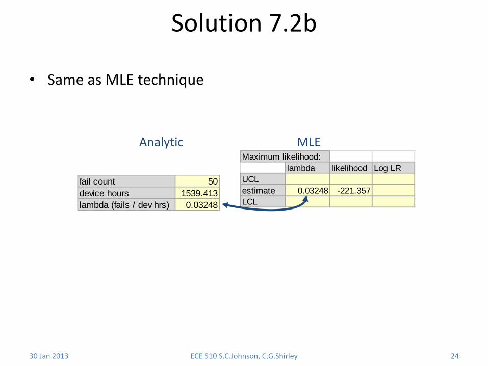
Solution 7.2b


• Same as MLE technique

Analytic MLE Maximum likelihood:


UCL

estimate 0.03248 -221.357

LCL

fail count 50

device hours 1539.413

lambda (fails / dev hrs) 0.03248

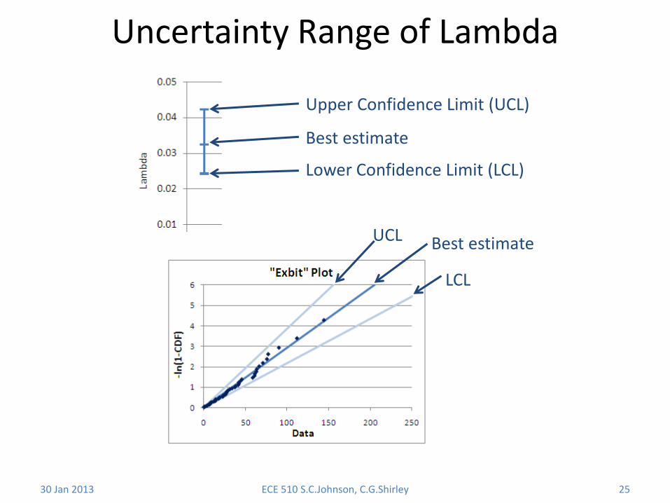
Uncertainty Range of Lambda


Best estimate UCL

LCL

Best estimate

Upper Confidence Limit (UCL)

Lower Confidence Limit (LCL)

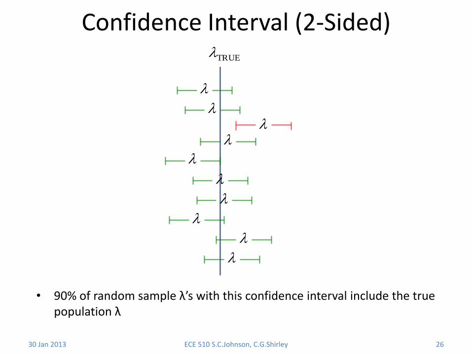
Confidence Interval (2-Sided)


• 90% of random sample λ’s with this confidence interval include the true population λ

TRUE

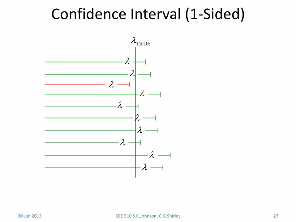
Confidence Interval (1-Sided)


TRUE

Uncertainties on Parameters


To calculate: • Monte Carlo • Likelihood ratio • Analytic

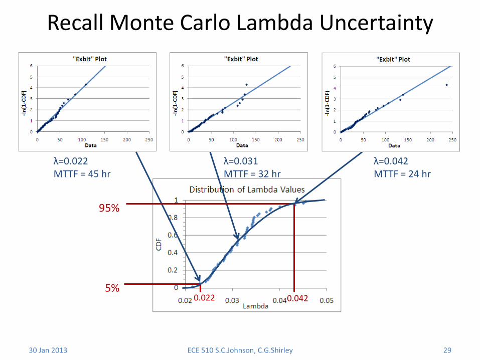
Recall Monte Carlo Lambda Uncertainty


5%

95%

0.022 0.042

λ=0.022 MTTF = 45 hr

λ=0.031 MTTF = 32 hr

λ=0.042 MTTF = 24 hr

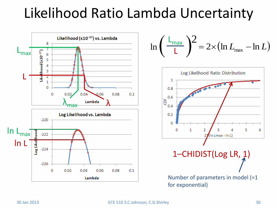
2Likelihood Ratio Lambda Uncertainty


λ λmax

Lmax

L

Lmax

L LL lnln2 max ln

ln L

ln Lmax

Number of parameters in model (=1 for exponential)

1–CHIDIST(Log LR, 1)

Maximum likelihood:


UCL 0.040632 -222.709 0.100001

estimate 0.03248 -221.357 1

LCL 0.025499 -222.709 0.100001

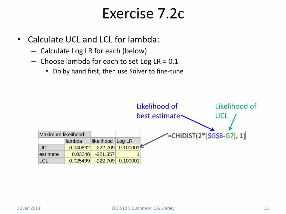
Exercise 7.2c


• Calculate UCL and LCL for lambda: – Calculate Log LR for each (below)

– Choose lambda for each to set Log LR = 0.1 • Do by hand first, then use Solver to fine-tune

Likelihood of best estimate

Likelihood of UCL

Maximum likelihood:


UCL 0.040632 -222.709 0.100001

estimate 0.03248 -221.357 1

LCL 0.025499 -222.709 0.100001

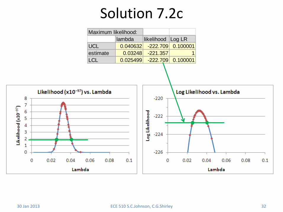
Solution 7.2c


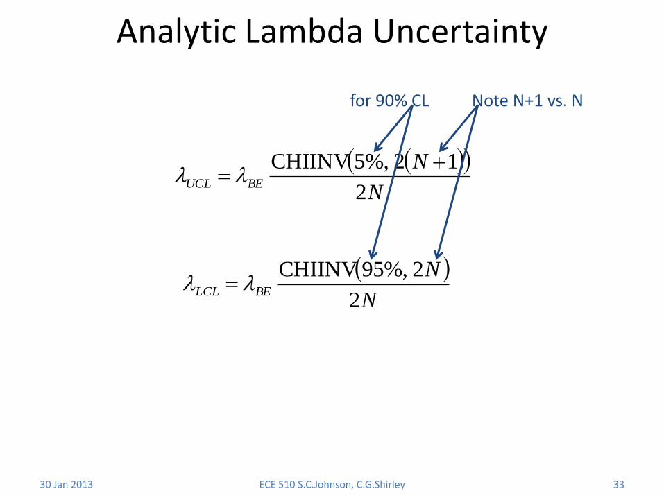
Analytic Lambda Uncertainty


N

NBEUCL

2

12%,5CHIINV

N

NBELCL

2

2%,95CHIINV

for 90% CL Note N+1 vs. N

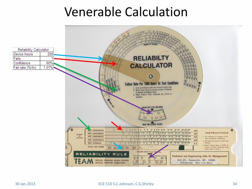
Venerable Calculation


Exercise 7.2d


• Calculate lambda UCL and LCL analyticall

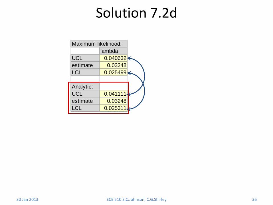
Maximum likelihood:

lambda

UCL 0.040632

estimate 0.03248

LCL 0.025499

Analytic:

UCL 0.041111

estimate 0.03248

LCL 0.025311

Solution 7.2d


Exercise 7.3


• This is Tobias & Trindade exercise 3.1

• How many units do we need to verify a 500,000 hr MTTF with 80% confidence, given that we can run a test for 2500 hours and 2 fails are allowed?

• Hint: you can do this by trial and error. Calculate the UCL on λ as a function of sample size SS and then adjust SS until the UCL equals the target λ.

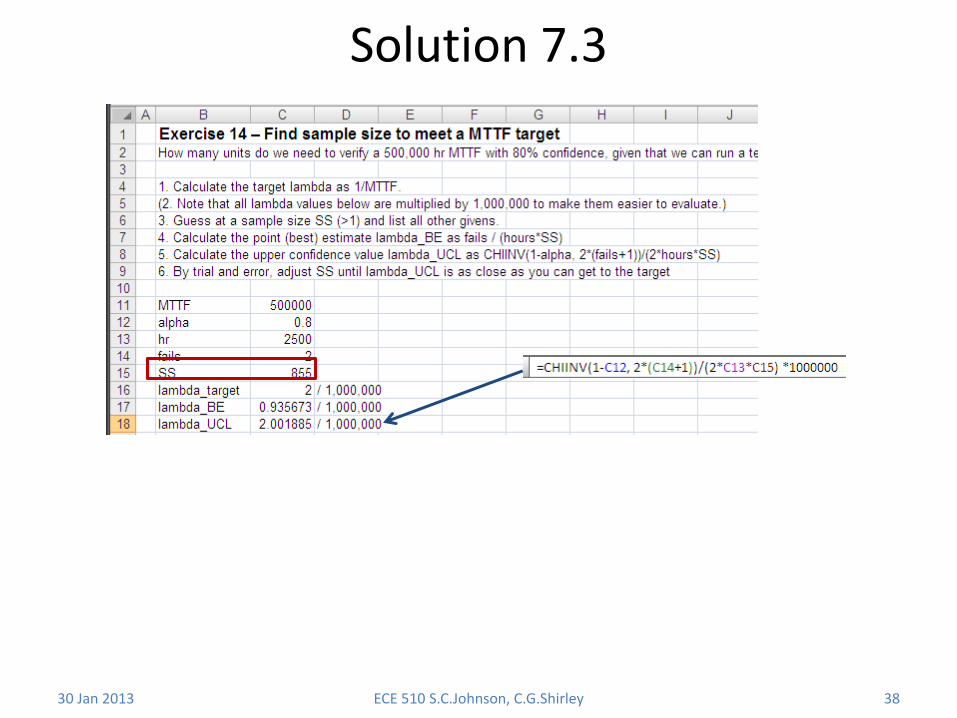
Solution 7.3


Normal Distribution MLE and Analytic


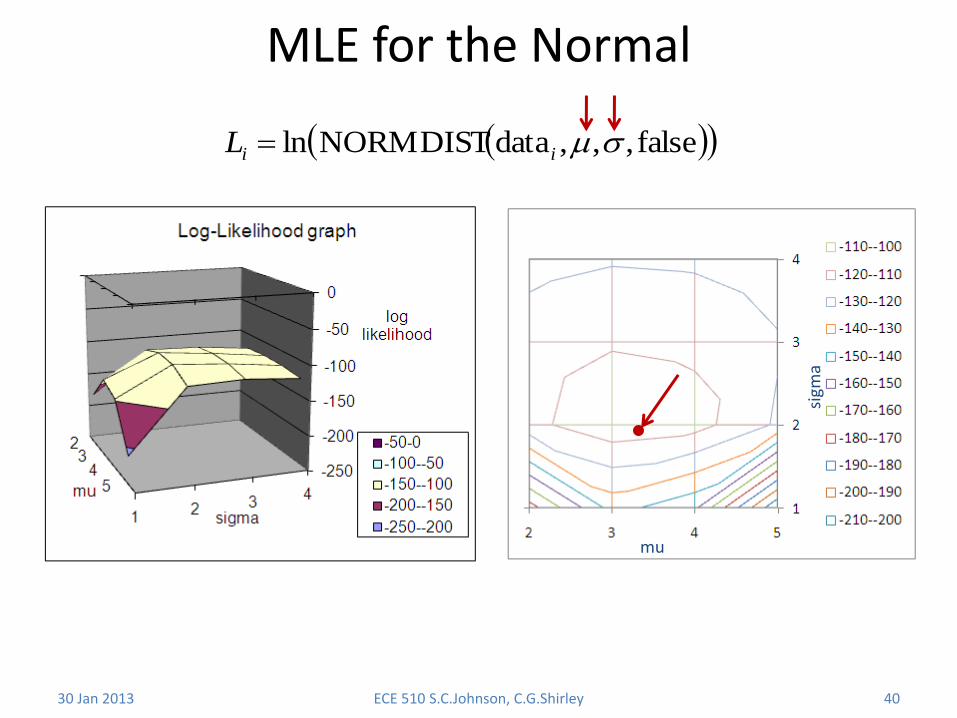
MLE for the Normal


false,,,dataNORMDISTln iiL

mu

sigm

a

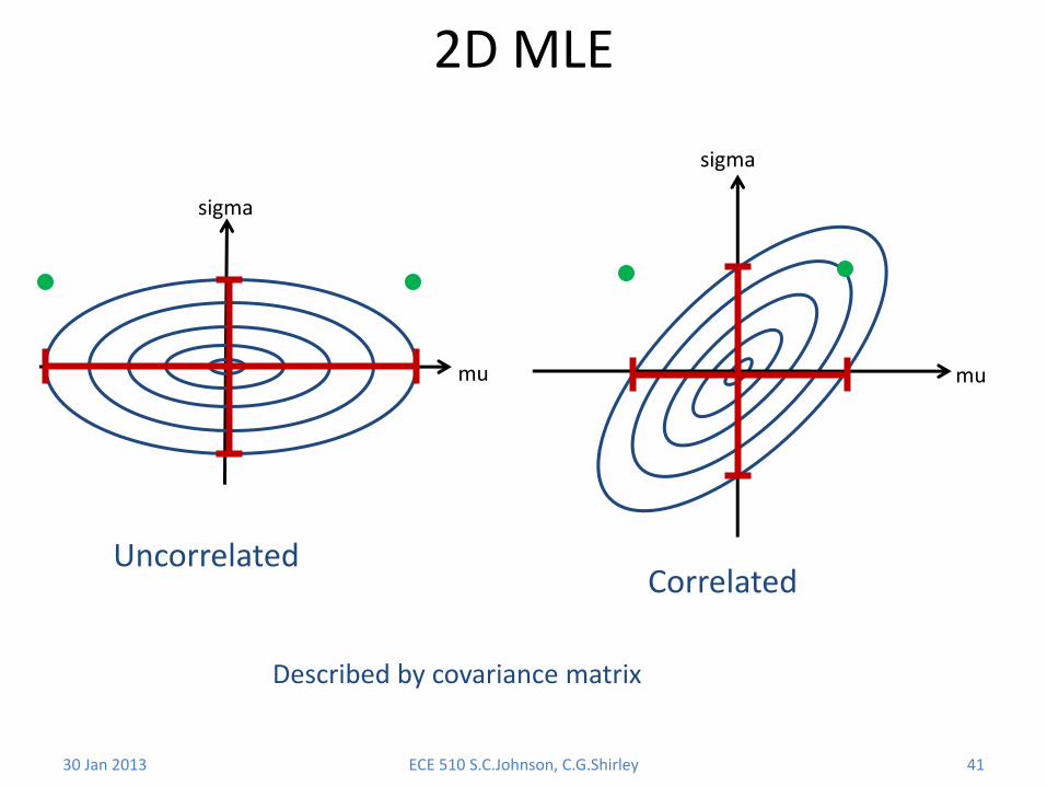
2D MLE


sigma

mu

Uncorrelated

sigma

mu

Correlated

Described by covariance matrix

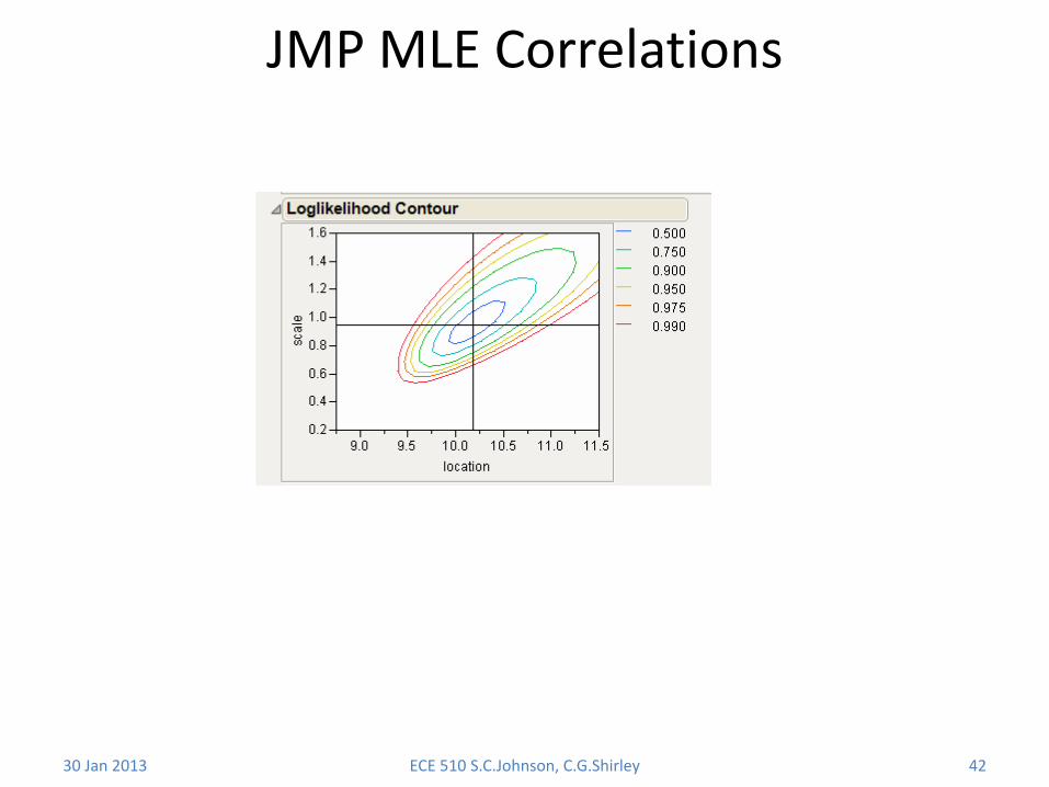
JMP MLE Correlations


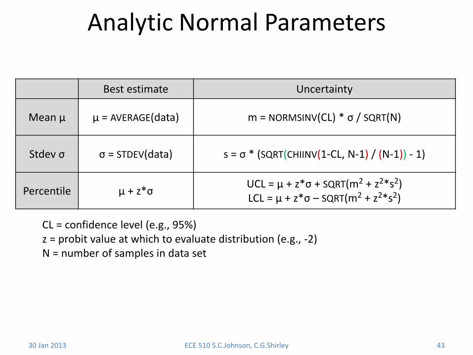
Analytic Normal Parameters


Best estimate Uncertainty

Mean µ µ = AVERAGE(data) m = NORMSINV(CL) * σ / SQRT(N)

Stdev σ σ = STDEV(data) s = σ * (SQRT(CHIINV(1-CL, N-1) / (N-1)) - 1)

Percentile µ + z*σ UCL = µ + z*σ + SQRT(m2 + z2*s2) LCL = µ + z*σ – SQRT(m2 + z2*s2)

CL = confidence level (e.g., 95%) z = probit value at which to evaluate distribution (e.g., -2) N = number of samples in data set

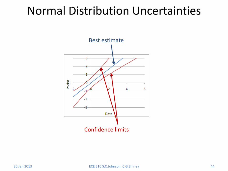
Normal Distribution Uncertainties


Best estimate

Confidence limits

Exercise 7.4a


• For the 9 data points given, extract mu, sigma, and their uncertainties, and calculate the 95% confidence interval for the 2-sigma point of their parent distribution.

Solution 7.4a


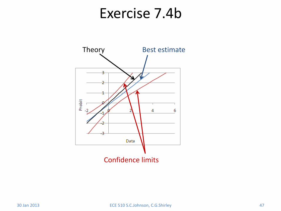
Exercise 7.4b


Best estimate

Confidence limits

Theory

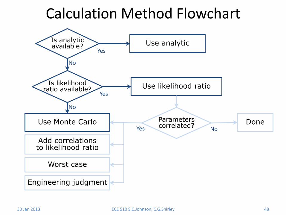
Calculation Method Flowchart


Is analytic available? Use analytic

Is likelihood ratio available? Use likelihood ratio

Use Monte Carlo

Yes

No

Yes

No

Parameters correlated? No Yes

Done

Add correlations to likelihood ratio

Worst case

Engineering judgment

Weibull MLE with Readout Data


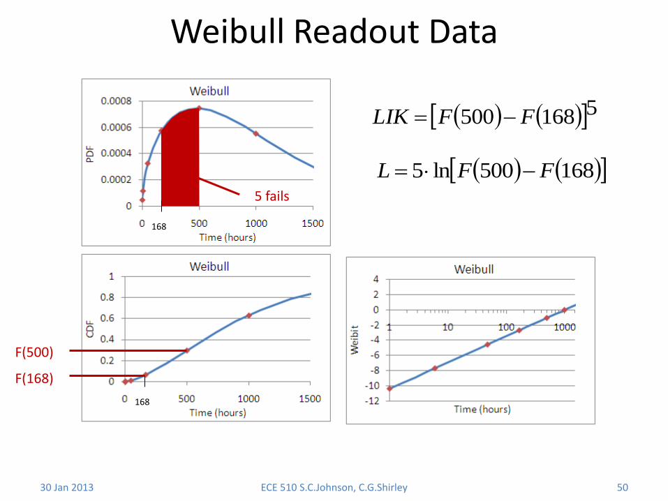
Weibull Readout Data


168

168

F(500)

F(168)

168500ln5 FFL

5168500 FFLIK

5 fails

MLE for Weibull


RR

R

r

rrrrr

tSs

tSdtFtFnL

ln

lnln1

1

ttF exp1

ttS exp

Vary these to maximize this

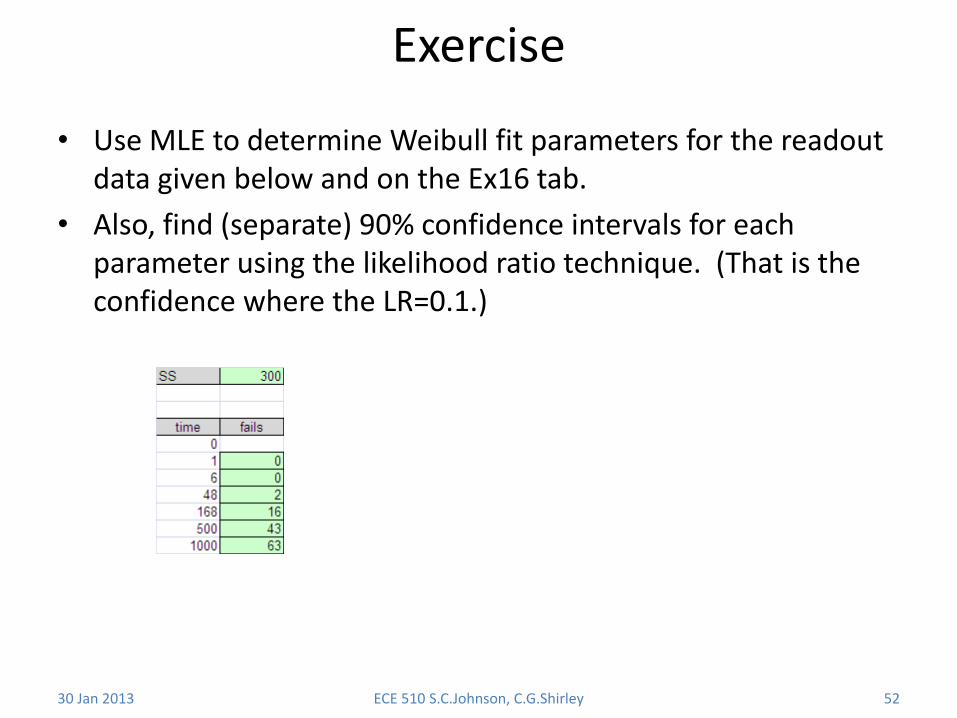
Exercise


• Use MLE to determine Weibull fit parameters for the readout data given below and on the Ex16 tab.

• Also, find (separate) 90% confidence intervals for each parameter using the likelihood ratio technique. (That is the confidence where the LR=0.1.)

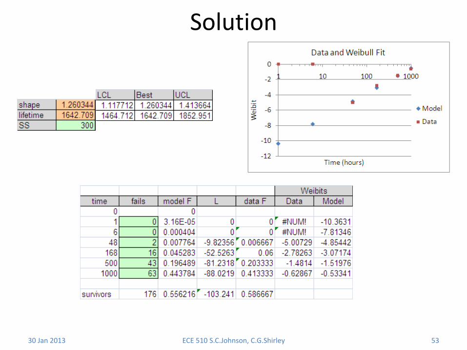
Solution


Exercise


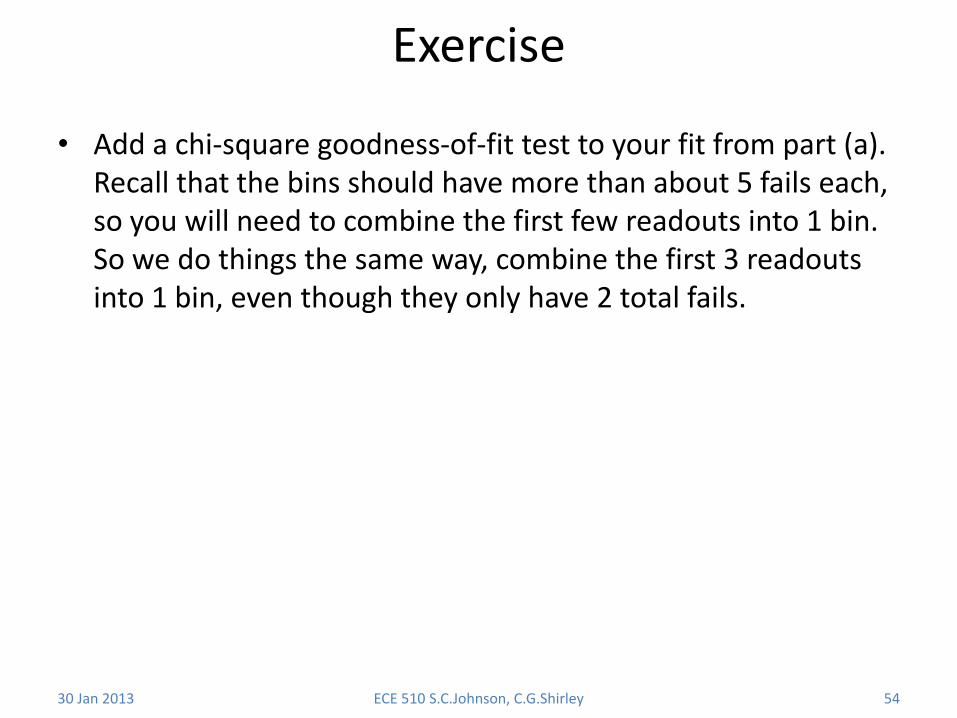
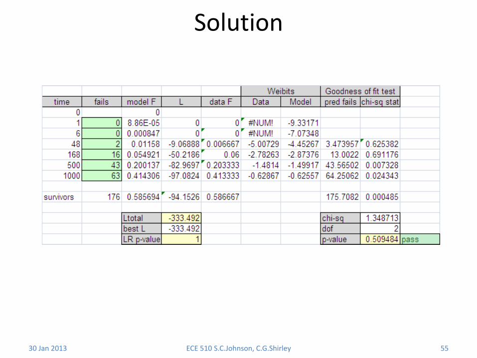
• Add a chi-square goodness-of-fit test to your fit from part (a). Recall that the bins should have more than about 5 fails each, so you will need to combine the first few readouts into 1 bin. So we do things the same way, combine the first 3 readouts into 1 bin, even though they only have 2 total fails.

Solution


Confidence and Figures of Merit


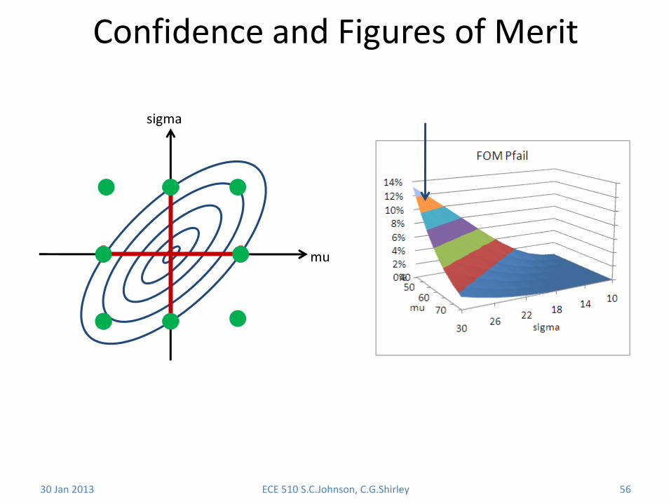
sigma

mu

Exercise


• Use the pfail at 2000 hours as the FOM for the Weibull model of Ex16. Evaluate this pfail as a function of the shape and lifetime parameters.

• Try various corners of the “space” of shape and lifetime values and find the worst case corner. Report these values as your worst case shape and lifetime values.

Solution


The End


ECE 510 Lecture 7 Confidence Intervals -...

Documents

Transcript of ECE 510 Lecture 7 Confidence Intervals -...