ECE 450 Lecture 1 - California State University, Northridgedvanalp/ECE 450/ECE 450...
31
ECE 450 D. van Alphen 1 ECE 450 – Lecture 1 “God doesn’t play dice.” - Albert Einstein “As far as the laws of mathematics refer to reality, they are not certain; as far as they are certain, they do not refer to reality.” - Albert Einstein • Lecture Overview – Announcements – Set theory review – Vocabulary: experiments, outcomes, trials, events, sample space – 3 axioms of probability – Combinatorics – Probability – what is it? (4 approaches) – EE Application: Information Theory
Transcript of ECE 450 Lecture 1 - California State University, Northridgedvanalp/ECE 450/ECE 450...

ECE 450 D. van Alphen 1
ECE 450 – Lecture 1
“God doesn’t play dice.”
- Albert Einstein
“As far as the laws of mathematics refer to reality, they are not certain; as
far as they are certain, they do not refer to reality.”
- Albert Einstein
• Lecture Overview
– Announcements
– Set theory review
– Vocabulary: experiments, outcomes, trials, events, sample space
– 3 axioms of probability
– Combinatorics
– Probability – what is it? (4 approaches)
– EE Application: Information Theory

Announcements
• Regular Office Hr: ______________________,
_______________________, JD 4414
• Syllabus Highlights
– Grading
– HW Due Dates
– Recorded Lectures and Tutorials
• Course Web Page: www.csun.edu/~dvanalp
(Follow links: Current Semester ECE 450)
ECE 450 D. van Alphen 2

ECE 450 D. van Alphen 3
Set Theory
• On your own time, review set complements, unions,
intersections, subsets, set differences, and Venn diagrams
from text, pp. 13 - 19
• Recall: Sets A and B are mutually exclusive (m.e., or
disjoint) iff: A B = F (the empty set).
• De Morgan’s Laws
(A B)’ = A’ B’
(A B)’ = A’ B’
• Recall that a set with n elements has _______ subsets.

ECE 450 D. van Alphen 4
Vocabulary for Probability
• An experiment is some action that has outcomes (z, zeta)
belonging to a fixed set of possible outcomes called the
“sample space” or the “universal set” or the “probability
space”, S.
– Each single performance of the experiment is called a
__________.
– Chance experiment = random experiment, denoted E
– Before performing the experiment, the actual outcome is
unknown;

ECE 450 D. van Alphen 5
Examples of Experiments
• Example 1: E1 = single toss of a die
– S = {__________________} (sample space)
– S is finite, countable
• Example 2: E2 = turning on radio receiver at time t = 0;
measure voltage at certain point in circuit, t seconds later;
define the outcome z(t) = v(t), where t is fixed;
– S = {v: - _____ < v < _____ } (sample space)
– uncountably infinite (ignoring measurement limits)

ECE 450 D. van Alphen 6
Examples of Experiments, continued
• Example 3: E3 : count the number of photo-electrons, (e),
emitted by a particular surface when a particular light beam
falls on it for t seconds; define the outcomes z0 : 0 e's
counted, z1 : 1 e counted, z2 : 2 e's counted, …
– S = { _________________ } countably infinite

ECE 450 D. van Alphen 7
More Probability Vocabulary
• Any subset of the sample space is called an ___________.
– Thus, A is an event if A S.
– The elements of the event, A, are the individual outcomes,
z, belonging to A.
• An experiment with n possible outcomes has
_______ events associated with it.
• Example 1, cont.' : A = “an odd # appears" = {_______}
B = “an even # appears" = {_______}
= A' (A-complement)

ECE 450 D. van Alphen 8
Examples of Events & More Vocabulary
• Example 2, cont.' : A = “voltage between 2 and 4, inclusive“
= {v: ___________________}
B = “voltage greater than 3" = {v: _________}
• Example 3, cont.‘ : A = “fewer than 4 e's counted"
= _____________________
B = “a negative # of e's counted“
= F (the null set or empty set)
• We say “event A occurs” whenever any outcome in A occurs
• Elementary events are those that consist of a single outcome;
compound events consist of several outcomes.

ECE 450 D. van Alphen 9
Axioms of Probability
• Axiomatic approach due to Kolmogorav (a Russian
mathematician, early 1900’s)
• A “probability” is a # assigned to an event, A, according to
three rules or axioms
– Axiom 1: Pr(A) _____ 0 (No negative probabilities)
– Axiom 2: Pr(S) = ____ (Something has to happen)
– Axiom 3: If A & B are m.e., then
Pr(A B) = _________________
• (For 2 m.e. events, probabilities are additive.)
• We say event A occurs with probability Pr(A)

ECE 450 D. van Alphen 10
Corollaries to the Axioms
• Corollary 1: Pr[A'] = 1 - Pr[A]
Proof: Pr(S) = Pr[A' A] = Pr(A') + Pr(A) (why? _______)
1 = Pr(A') + Pr(A) (why? ________________)
Pr(A') = 1 - Pr(A)
• Example: Consider a 52-card deck.
Pr(ace) = 4/52 = 1/13 (since there are 4 aces in the deck)
Pr(not getting an ace) = Pr(2, 3,…, 10, J, Q, K)
= 1 - __________ = ______ (by cor. 1)
Note that the events {ace} and {2, …, 10, J, Q, K} are complementary events

ECE 450 D. van Alphen 11
Corollaries, continued
• Corollary 2: 0 ____ Pr(A) ____ 1
Proof: Ax. 1; Pr(A) = 1 - Pr(A') (Cor. 1)
___ 0 (Ax. 1)
____ 1
• Corollary 3: Pr(F) = 0
Proof: Pr(S) = Pr(S F) = Pr(S) + Pr(F) (since S, F m.e.)

ECE 450 D. van Alphen 12
Corollaries, continued
• Corollary 4: Pr(A B) = Pr(A) + Pr(B) - Pr(A B)
Proof: Pr(A B) = Pr(A (B A’)) = Pr(A) + Pr(B A’)
(m.e.) (1)
Venn Diagram:
A B
(to be
completed
in class)
S

ECE 450 D. van Alphen 13
Corollaries, continued
• Similarly:
Pr(B) = Pr((A B) (A’ B)) = Pr(A B) + Pr(B A’)
(m.e.) (2)
• Venn Diagram:
• Now subtract equation (1) from equation (2):
Pr(B) - Pr(A B) = Pr(A B) - Pr(A) (proving cor. 4)
A B
(to be
completed
in class)
S

ECE 450 D. van Alphen 14
Example (verifying the corollary)
• Experiment: Toss one die; Find Pr(A B) for A, B below:
Let A = {1, 3} , B = {3, 5} Note: A B = {3}
Pr(A) = Pr({1} {3}) = Pr{1} + Pr{3} = 1/6 + 1/6 = 1/3
Similarly, Pr(B) = 1/3
Pr{1, 3, 5} = Pr(A B) = Pr(A) + Pr(B) - Pr(A B)
= 1/3 + 1/3 - Pr{3} = 1/3 + 1/3 - 1/6
= 3/6 = ½ (agreeing with our intuition)
ECE 450 D. van Alphen 15
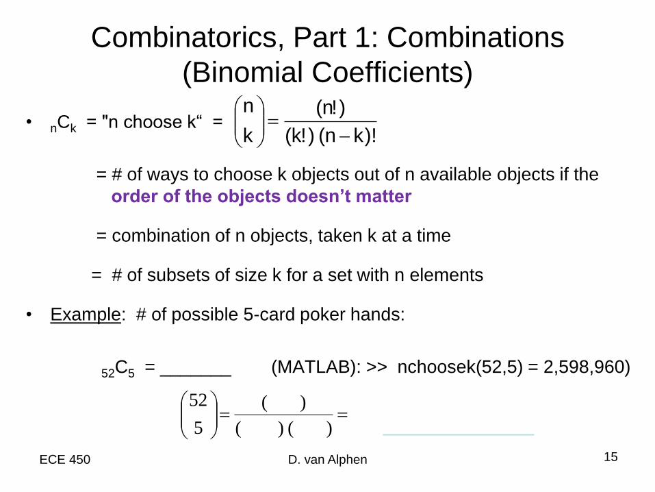
Combinatorics, Part 1: Combinations
(Binomial Coefficients)
• nCk = "n choose k“ =
= # of ways to choose k objects out of n available objects if the
order of the objects doesn’t matter
= combination of n objects, taken k at a time
= # of subsets of size k for a set with n elements
• Example: # of possible 5-card poker hands:
52C5 = _______ (MATLAB): >> nchoosek(52,5) = 2,598,960)
)!kn()!k(
)!n(
k
n
)()(
)(
5
52

ECE 450 D. van Alphen 16
Combinatorics Example: 5-card Poker
• Example: Pr(3 Spades in 5-card poker hand)
=
numerator = # ways to choose 3 Spades and 2 non-Spades
denominator = # of possible 5-card poker hands
082.52
3913
ECE 450 D. van Alphen 17
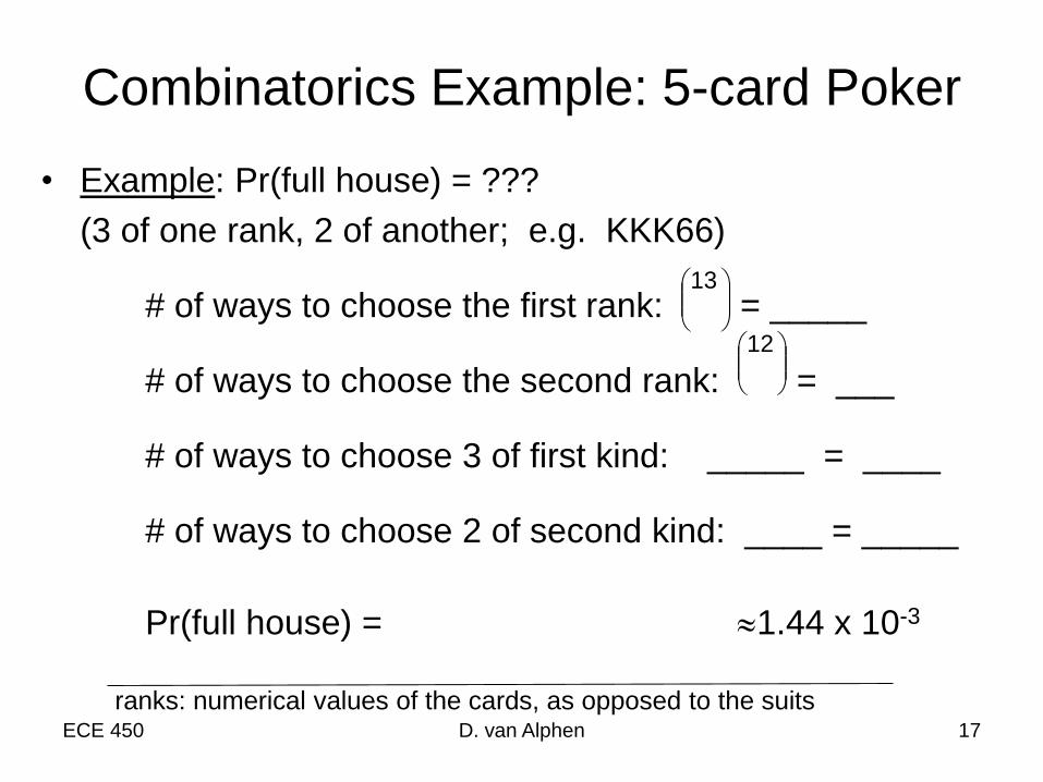
Combinatorics Example: 5-card Poker
• Example: Pr(full house) = ???
(3 of one rank, 2 of another; e.g. KKK66)
# of ways to choose the first rank: = _____
# of ways to choose the second rank: = ___
# of ways to choose 3 of first kind: _____ = ____
# of ways to choose 2 of second kind: ____ = _____
Pr(full house) = 1.44 x 10⁻³
13
12
ranks: numerical values of the cards, as opposed to the suits

ECE 450 D. van Alphen 18
Combinatorics, Part 2: Permutations
or Arrangements
• nPk =
= permutation of n objects taken k at a time
= # of ways to arrange k out of n objects, assuming that
the order matters
• Example 1: # of possible license plates if they are formed
from 26 letters of the alphabet and are 5 letters in length,
and no letter can be repeated
26P5 = 26!/21! = 26 • 25 • 24 • 23 • 22 = 7,893,600
)!kn(
!n
ECE 450 D. van Alphen 19
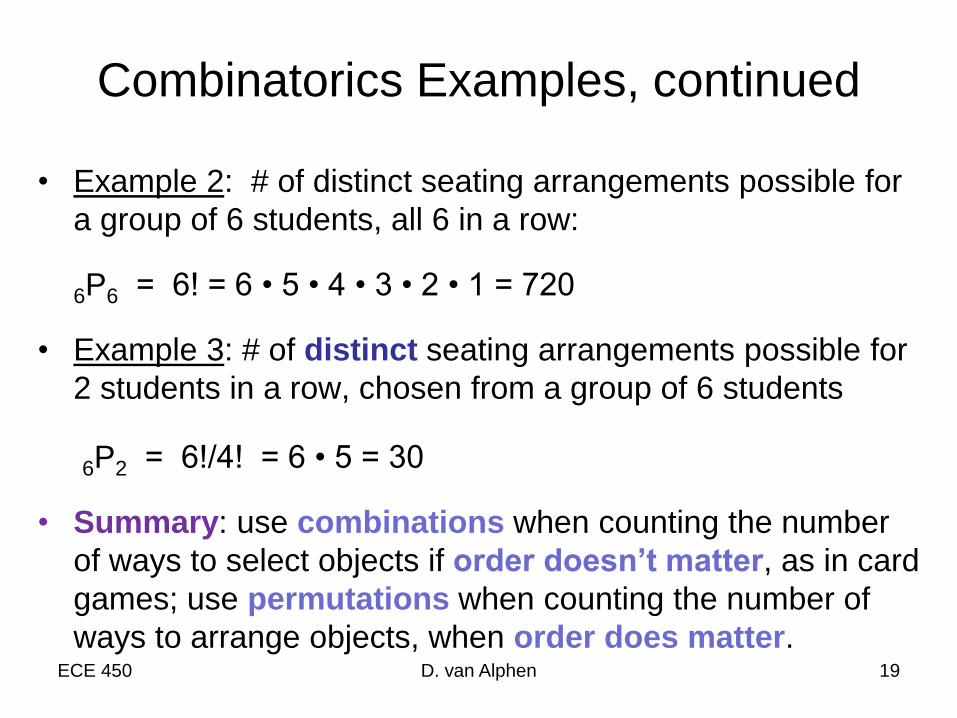
Combinatorics Examples, continued
• Example 2: # of distinct seating arrangements possible for
a group of 6 students, all 6 in a row:
6P6 = 6! = 6 • 5 • 4 • 3 • 2 • 1 = 720
• Example 3: # of distinct seating arrangements possible for
2 students in a row, chosen from a group of 6 students
6P2 = 6!/4! = 6 • 5 = 30
• Summary: use combinations when counting the number
of ways to select objects if order doesn’t matter, as in card
games; use permutations when counting the number of
ways to arrange objects, when order does matter.

ECE 450 D. van Alphen 20
Interpretations of Probability:
A. Classical Concept
• The classical concept assumes all outcomes are equally
likely
Pr(A) =
• Justified (for some problems) by the “Principle of
Indifference” or “Maximum Ignorance”: no reason to favor
one outcome over another
• Usually applied to gambling problems: dice, cards, coins, …
• Example: Pr(bridge hand of 13 cards out of 52 has exactly
one ace); solution follows
Sinoutcomespossibleof#
Ainoutcomesof#

ECE 450 D. van Alphen 21
Classical Probability: Example
• Pr(bridge hand of 13 out of 52 cards has 1 ace)
=
= = .439
handsbridgepossibleof#
ace1exactlywithhandsbridgeof#

ECE 450 D. van Alphen 22
Interpretations of Probability:
B. Relative Frequency Concept (von Mises)
• Repeat an experiment N times; suppose (for example) that
there are 4 possible outcomes, or elementary events, called
A, B, C, and D.
• Let NA be the # of times event A occurs; similarly define NB,
NC, and ND.
• Clearly, N = NA + NB + NC + ND.
• Define the relative frequency of event A as: r(A) = NA/N
• Relative frequency approach: )(lim)Pr( ArAN
ECE 450 D. van Alphen 23
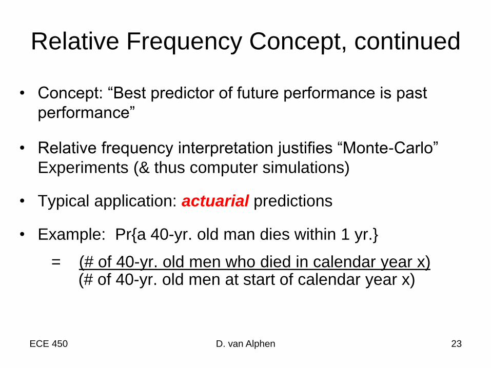
Relative Frequency Concept, continued
• Concept: “Best predictor of future performance is past
performance”
• Relative frequency interpretation justifies “Monte-Carlo”
Experiments (& thus computer simulations)
• Typical application: actuarial predictions
• Example: Pr{a 40-yr. old man dies within 1 yr.}
= (# of 40-yr. old men who died in calendar year x)(# of 40-yr. old men at start of calendar year x)
ECE 450 D. van Alphen 24
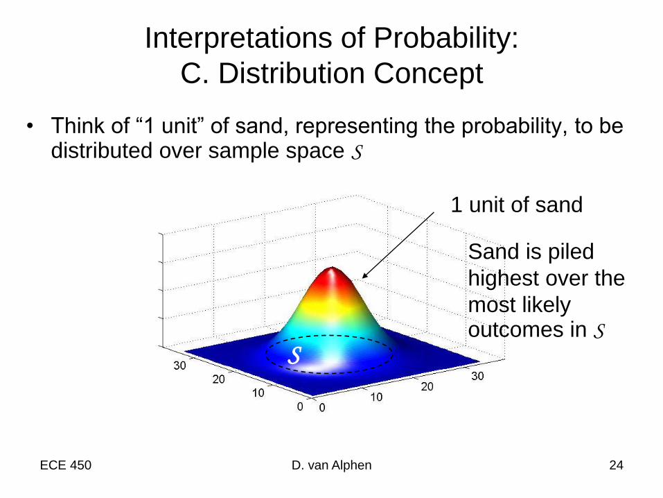
Interpretations of Probability:
C. Distribution Concept
• Think of “1 unit” of sand, representing the probability, to be distributed over sample space S
S
1 unit of sand
Sand is piled
highest over the
most likely outcomes in S

ECE 450 D. van Alphen 25
Interpretations of Probability:
D. Measure of Likelihood View
• Probability is a function whose domain is the sample space
and whose range is the set of real numbers between 0 and
1:
Impossible events 0
Unlikely events near 0
Very likely events near 1
Certain events 1

ECE 450 D. van Alphen 26
EE Application: Information Theory
(Subset of CommunicationTheory)
• Channels can only accommodate so much information ( There exists an information capacity and maximum rate.)
• How do we “measure” information?
• Some concepts:
– Communication of information prior uncertainty (Ex: whistle the musical note F#)
– Prior uncertainty about outcome
“surprise“ on occurrence of event
• e.g., ask: “Will I believe in n years?”
ECE 450 D. van Alphen 27
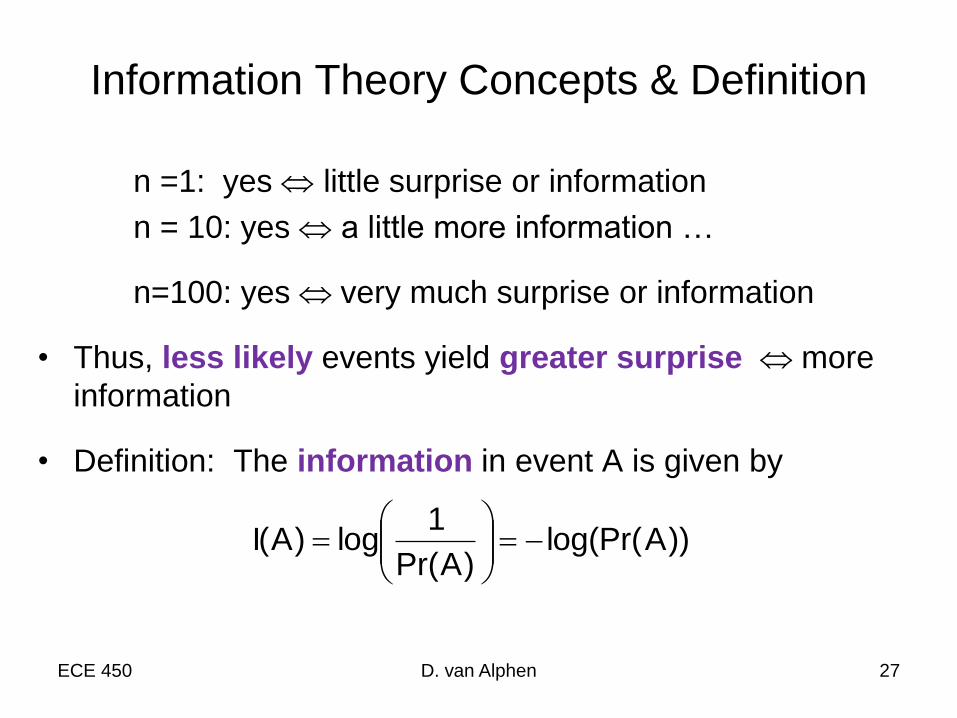
Information Theory Concepts & Definition
n =1: yes little surprise or information
n = 10: yes a little more information …
n=100: yes very much surprise or information
• Thus, less likely events yield greater surprise more
information
• Definition: The information in event A is given by
))Alog(Pr()APr(
1log)A(I

ECE 450 D. van Alphen 28
Information, continued
• Units of measure for information in event A:
I(A) = - Log[Pr(A)] bits if log is base 2
nats if log is base e (natural log)
hartleys if log is base 10 (common log)
Example 1: Binary Alphabet, S = {0,1}
(Think of communicating a string of 1's and 0's, say ASCII,
where 1's and 0's are equally likely.)
Symbol, s Pr(s) I(s)
0 ½ Log2(___) = 1 bit
1 ½ Log2(___) = 1 bit
Average info. per symbol:
1 bit

ECE 450 D. van Alphen 29
Information, continued
• Example 2: Binary Alphabet, S = {0,1}
• This time we'll still send a stream of 1's and 0's, but they are
not equally likely; say Pr(0) = ¼, Pr(1) = ¾
• Recall: To convert logs from one base to another –
logb(x) = ________________
Symbol, s Pr(s) I(s)
0 ¼ Log2(___) = __ bits
1 ¾ Log2(__/__) = .42 bits
Average info. per symbol:
1/4(2) + 3/4(.42) = .815 bits

ECE 450 D. van Alphen 30
Information & Entropy
• Definition: The entropy of the source, S, is the average
information per symbol, given by
H(S) =
sym. info. prob(symbol)
• For our examples
– Equally likely symbols H(s) = 1 bit/symbol
– Pr(0) = ¼ , Pr(1) = ¾ H(s) = .815 bits/symbol
Ss
)sPr()s(I Due to bandwidth
constraints, a source
with a large entropy
is desirable.
Review
• Pr(A B) = __________________________________
(general rule)
• Pr(A’) = ______________________
• Combination of n things taken k at a time: ______ = _____________
• Information in the event A, I(A) = ____________________
• Entropy in source S with symbols s: H(S) = ______________
ECE 450 D. van Alphen 31


