ECE 3511: Communications Networks “Theory and Analysis ...

ECE 3511: Communications Networks“Theory and Analysis”

Fall Quarter 2002

Instructor: Prof. A. Bruce McDonald

Lecture Topic

Introductory Analysis of M/G/1 Queueing Systems

Module Number One

Steady-State System Behavior—The Recursion Approach

ECE 3511 Fall 2002; Prof A. Bruce McDonald 2

Fundamental Queueing Theory

Equilibrium Behavior of the M-G-1 Queueing System

Using the Recursion Approach to Solve the P-K Formula

Poisson Arrivals with General Service:

In this module students are introduced to a queueing system inwhich the arrivals are assumed to be Poisson, but, only the firstand second of moments of the general service time distribution isknown—the entire distribution need not be know in order to solvefor the steady-state behavior of the system.

In the following analysis it is assumed that customers are served ina FIFO manner and that Xi is the service time of the ith customer.The constraint is that the set of random variables (RVs) (X1; X2; : : :)are IID (mutually independent and identically distributed) and theyare indenpendent of the interarrival times.

Some Notation

� � = Mean Customer Arrival Rate (Poission Process)

� � = Mean Customer Service Rate (General Distribution)

� � = ��= Average System Utilization

� X = E[X] = 1

�= Average Service Time

� � = Variance of the Customer Service Times

� X2 = E[X2] = Second Moment of the Service Time

� �i = Equilibrium Probability there will be i Customers in the System


The M/G/1 Queueing System

� MG1 is a Single Queueing System

� Customer Arrivals Characterized by a Poisson Process;

� Service Times are Characterized by an Arbitrary Distribution;

� Results are given by the (Pollaczek-Khinchin) P-K formulas:

� First: Find P-K formula for the mean number in the system;

� Using a transform equation the P-K formula is utilized to derivethe equilibrium state probabilities;

n n+1 n+2 n+3n−1n−2

k

k

k

k

0

2

3

4

k1

Figure 1: M/G/1 queueing system showing the imbedded Markov Chain.

Recursion Approach:

To find the mean number in the system start with a difference equation for the number in thesystem following the ith departure. The expected value of the square of the resulting expressionis the P-K mean value formula—The key assumption, is that the state probabilities at departureinstants are equal to the equilibriumm probabilities 1 This characteristic is the basis for theimbedded Markov Chain, as shown for departure instants, of the M/G/1 system in Figure-1.

1This observation is proven later.


The M/G/1 Recursion for Departure Instants

Number in System

Continuous Time (t)

FirstDeparture

SecondDeparture

ThirdDeparture

n0 = 0

n1 = n0 � 1 + a1 = 2

n2

n3

a2 = 3 (Number of arrivals between 1st and 2nd departure)

Figure 2: Sample path of M/G/1 system state at departure instants.

� Consider the system “state” at the departure instants;

� Define ni+1 as the number in the system immediately followingthe (i+ 1) st departure;

1. ni+1 enumerates the customers in the queue and in service;

2. ni+1 is also equal to the number of customers in the system after theith departure minus 1 (since there must have been one-and-only-onedeparture, plus the number of customer arrivals between the ith and the(i + 1) st departure;

� Define ai+1 as the number of customers that arrive to the systembetween the i th and the (i+ 1) st departure instants.

ni+1 = ni � 1 + ai+1 ; ni > 0 (1)


Special Case: The Empty Queueing System

Empty Sytem: The number in the system immediately followingthe departure of the i+1 st customer 2 for the cases in which ni = 0will be equal to the number of arrivals during the service time of thearrival of the first customer to the empty system.

ni+1 = ai+1 ; ni = 0

The unit step function provides a nice way to express the separaterecursions as a single equation as follows:

ni+1 = ni � u(ni) + ai+1

Wherein the step function is defined as:

u(ni) = f1; ni > 00; ni = 0

2Commonly refered to as the i+ 1 st departure instant.


The Second Moment of the State Equation

Methodology: Based on the recursion approach taken here theP-K formula can be found by, first, squaring both sides of the re-cursion equation, and, then, taking the expected values—in thiscase second moments because of the square.

n2i+1 = f(ni � u(ni) + ai+1)

2

n2i + u(ni)2 + a2i+1 � 2niu(ni) + 2niai+1 � 2u(ni)ai+1

Now take the expected value of both sides:

E[n2i+1] = E[n2i ] + E[u(ni)2] + E[a2i+1] (2)

�2E[niu(ni)] + 2E[niai+1]� 2E[u(ni)ai+1] (3)

The P-K Formula: The desired result is a useable equation for thesteady-state number of customers in the queue, which, is simplyE[ni]. Hence, to find the equilibrium behavior of an M-G-1 queueingsystem the strategy is to restate the equation given above term-by-term and then to solve the simplified equation for E[ni].

Objective:

P �K formula! E[ni]


Term-by-Term Simplification for P-K Evaluation EquivalentMoments

Steady-State Equivalents: The objective of this analysis is thecharacterize the steady-state behavior of an ergodic system. Underequilibrium conditions the k th moment of any state variable, S, willbe equal 8i; j 2 steady-state: E[Sk

i ] = E[Skj ], hence, the following two

terms should be equal and cancel in the equation:

E[(ni+1)2] = E[n2i ] (4)


Term-by-Term Simplification for P-K Evaluation

Properties of the Unit Step Function

Product Equivalence: Since the Unit Step is either equal to 0 or1 it is clear that for any state variable S, state i, and powers m;n:u(Si)

m = u(Si)n; therefore u(ni) = u(ni)

2, hence, the expected valueswill also be equal:

E[u(ni)] = E[u(ni)2]

Finding the expectation for E[u(ni)]: What is required is a moreuseful expression for E[u(ni)]. Here, the theory of total probabil-ity and a very general queueing result for busy systems provide astraight forward solution:

E[u(ni)] =1X

n=0

u(ni)Pr[ni = n]

E[u(ni)] =1X

n=0

Pr[ni = n]

E[u(ni)] = Pr[System is Busy]



Using System Busy Time to Eliminate the Unit Step Function

Finding the System Busy Time: In an ergodic system understeady-state it is easy to determine the probability of the systembeing busy by considering an arbitrary interval of time � and us-ing probability to characterize the fraction of the interval that therewill be one or more customers in the system, i.e. the system will bebusy. If �b is the busy time then:

�b = � � ��0

Customer Service: For any probability distribution for servicetimes the mean service rate � is known—it is the inverse of thefirst moment, or expected value of the service time for the givenM-G-1 system: X. The number of customers served in the busyinterval �b is:

(� � ��0)�

Global balance can be applied, which, reflects that on average thenumber of customers served in an arbitrary interval is equal to thenumber of customers that arrive in the same interval:

�� = (� � ��0)�

� = 1� �0

E[(u(ni)2] = E[u(ni)] = Pr[System is Busy] = 1� �0 = � (5)



Additional Sundry Results

� Since niu(ni) = ni—the following simplification:

2E[niu(ni)] = 2E[ni] (6)

� The number of customers that arrive to the system betweenthe i th and the i + 1 st departure instants (ai+1) is indepen-dent of the number in the system after the i th departure sys-tem (ni). Hence, by idependence the following simplification be-comes possible:

E[u(ni)ai+1] = E[u(ni)]E[ai+1]

By Equation-5 it is shown that E[u(ni)] = �, hence, it is possibleto further simplify this equation by determining the value ofE[ai+1] by returning to the original recurance relation (Equation-1 and taking the expectation of both sides:

E[ni+1] = E[ni] + E[u(ni)] + E[ai+1]

After rearranging terms and making all necessary substitutionsthe following result is obtained:

2E[u(ni)ai+1] = 2E[u(ni)]E[ai+1] = 2�2 (7)

� Finally, the same argument leads to similar simplification of thefinal term:

2E[niai+1] = 2E[ni] = 2E[ni]� (8)


Equilibrium Solution for the M-G-1 Queue

The P-K Formula for the Mean Number in the Queue

The results derive for each term can be substituted into Equation-2, which can then be solved for the desired quantity: E[ni], which, isthe expected value of the number in the system at the i th departureinstant:

E[ni] =�+ E[a2i+1]� 2�2

2(1� �)

Departure Instants = Any Instant: Using the initial assumptionthat expected values at the departure instants are equivalent thethe expected values at equilibrium, and, hence, any instant thefollowing relation holds:

E[ni] = E[n]

Stationarity of the Poisson Process: The final result follows byobserving that a time homogeneous Poisson Process has both in-dependent increments and stationary increments. Hence, the fol-lowing relation holds:

E[a2i+1] = E[a2]

The P-K Formula:

E[n] =�+ E[a2]� 2�2

2(1� �)(9)


Equilibrium Solution for the M-G-1 Queue

Some Useful Results from Probability and Statistics

The problem with Equation-9 is that knowledge of the second mo-ment of the service distribution may not be readily available. Hence,a better expression would require knowledge of only three (3) sys-tem parameters:

1. The mean arrival rate

2. The mean service rate (or time)

3. The variance of the service time distribution

The required results are as follows 3:

� V AR[X] = E[X2]� E[X]2

� V AR[Y ] = E[V AR[Y jX]] + V AR[E[Y jX]] 4

The remaining details of the derivation are left for the student towork out. The important intermediate result (students should con-firm) is:

E[a2] = �+ �2�2s + �2

3X and Y are arbitrary RV4Convince yourself of these two general results.


The Pollaczek-Khinchin Mean Value Formula

Results for the M-G-1 Queueing System

Bringing Everything Together: One form of the P-K mean valueformula is given as follows:

E[n] =2�� 2 + �2�2s

2(1� �)(10)

Some algebraic manupulation and application of Little’s Law bringabout some variations for of the same result:

E[n] = �+�2 + �2�2s2(1� �)

(11)

= �+�2X2

2(1� �)(12)


Other Approaches for MG1 Systems

Next: Using Residual Service Time

� Regeneration Instants: The recursion approach is a usefulstrategy for solving for the steady-state number in the system ifthe system exhibits regeneration points.

� In a Markovian system the state transitions provide these points.

� How does this help in the M-G-1 System? (More on this later)

� Unfinished Work Process: The residual work at time t is thetime it would take to empty out the queue assuming there areno additional arrivals after time t.

– In general this approach requires the arrival and service timedistributions.

– For the M-G-1 the first and second moments of the servicetime are sufficient.

– Finding the distribution of the unfinished work is all that isneeded to find everything about the system.

ECE 3511: Communications Networks“Theory and Analysis”

Fall Quarter 2002


Lecture Topic


Module Number Two

Steady-State System Behavior—The Residual Work Approach




Using Residual Service Times to Derive and Understand the

Pollaczek-Khinchin (P-K) Formula

Some Notation

� Wi = Waiting time of the ith customer

� Ri = Residual service time as seen by the ith customer

� Xi = Service time of the ith customer

� Ni = Number of waiting customers at the ith customer arrival

� R = Mean residual waiting time (R = limi!1E[Ri])

� NQ = Mean number of customers in the queue

ith Customer

jth Customer

Service Time (Xj)

Waiting Customers (Ni)

Residual Service (Ri)

Figure 1: Illustration of residual service seen by the ith customer.


What is the Residual Service Time?

Definition of Residual Service Time

� If customer j is being served when customer i arrives, Ri is thetime remaining until j’s service is complete.

� If the system is empty then Ri = 0.


Derivation of the P-K Formula

� Waiting time for the ith Customer:

Wi = Ri +i�1X

j=i�Ni

Xj

� Take the expectation of both sides and condition Xj on Ni:

E[Wi] = E[Ri] + E[i�1X

j=i�Ni

Xj]

= E[Ri] + E[i�1X

j=i�Ni

E[XjjNi]] (1)

� Recall from Probability that: E[X] = E[E[XjY ]]; Work this out toconvince yourself;

� Furthermore, Ni is independent of Xk8k 2 (i � 1; i�Ni) , hence,Equation-1 can be re-written:

E[Wi] = E[Ri] +XE[Ni]

� Take the limit of each side as i!1:

limi!1

E[Wi] = W = R+1

�NQ (2)


A Nice Property of Poisson Arrivals

� PASTA Property: This result assumes that NQ and R as ob-served by an arriving customer are equal to the mean valuesobserved from outside the system at a random time.

Poisson-Arrivals-See-Time-Averages


Determining the Mean Residual Service Time

Graphical Argument

t0

X1 X2 XM(t)

Res

idu

alS

ervi

ceT

ime

r(�)

Time �

Figure 2: Graphical Representation of Mean Residual Time.

� Consider the time average of the residual service time, r(�), dur-ing the interval [0; t]

� Let M(t) be the number of service completions up to time t

1

t

Z t

0r(�)d� =

1

t

M(t)Xi=1

1

2X2

i

=1

2

M(t)

t

PM(t)i=1 X2

i

M(t)(3)


Determining the Mean Residual Service Time

Continued

� Assuming that the process is ergodic time averages can be re-placed by ensemble averages!

� Determine the time average first;

� Take the limits of both sides of Equation-3 as t!1 :

limt!1

1

t

Z t

0r(�)d� =

1

2: limt!1

M(t)

t: limt!1

PM(t)i=1 X2

i

M(t)

� On the left is the time-average of the residual service time: R

� The 1st limit on the right is the time-average of the service com-pletion rate, which equals the arrival rate: � (WHY?)

� The 2nd limit on the right is the second-moment of the servicetime: E[X2

i ]

� Based on the ergodic assumption:

R =1

2�X2 (4)


Evaluating the P-K Formula

� Substituting the result for the expected value of the residualwork given in Equation-4 into Equation-2:

W =1

2�X2 +

1

�NQ

� But what is the value of the mean number in the queue (NQ)seen by an arrival ?

� Based on the PASTA property defined earlier it is the typicalvalue at an arbitrary instant—the expected value! Hence, byLittle’s Law:

NQ = �W

W =1

2�X2 + �W

=�X2

2(1� �)(5)

ECE 3511: Communications NetworksTheory and AnalysisFall Quarter 2002


Lecture Topic:


Module Three:

M-G-1 Examples Using the P-K Formula

1




Some Examples from the P-K Mean Value Formula

0 5 10 15 200

20

40

60

80

100

Mean Interarrival Time (Poisson)

Mea

n W

aitin

g T

ime

in Q

ueue

MG1 Queue: Waiting Time Versus Load (Mean Service Time = 50)

Figure 1: Effect of Incresing the Variance in Service Time with MG1 System.

� How is the mean waiting time determined?

� Try applying Little’s Law

Using the recursion approach the P-K Mean Value Formula was derived for the number of cus-tomers in the system. Application of Little’s Law and some algebraic manipulation transforms itinto the more commonly used form that specifies the mean waiting time in the queue—the formthat is derived directly when using the residual service time approach.



The MD1 Queueing System

Deterministic Service Times: The M-D-1 Queue

Poisson Arrivals (� packets/sec) Transmission Rate (C bits/sec)

Fixed Length Packets (L bits/packet)

Figure 2: Example of an MD1 System—Based on Fixed Packet Lengths.

MG1 results provide a nice metholdology to gain insight regardingbehavior of systems that use fixed packet lengths 1.

� Fixed length packets transmitted on a channel with a constanttransmission rate will all be serviced in precisely the same time:That time is also the mean and the variance will be zero. Hence,for the MD1 system:

E[n] = �+�2

2(1� �)

� Assuming IID Exponentially Distributed service times the P-KMVF reduces (as it should) to the well known MM1 result:

E[n] =�

(1� �)

1NOTE: Be careful not to confuse “service rate” with the transmission rate...Convince yourlself you understand the difference!


Comparison of MD1 and MM1 Systems

With some algebraic manipulation one can show that the meannumber in the system for an MD1 queue is always going to be lessthan the mean number in an MM1 queue given the same arrivalrate and mean packet length (assuming the transmission rate isfixed). For the MD1 queue the P-K formula can be re-written as:

E[n](MD1) =�

(1� �)�

�2

2(1� �)= E[n](MM1) �

�2

2(1� �)

Under backlogged conditions, i.e., as � ! 1, it can be shown 2

that the delay for the MM1 system approaches twice that for the“equivalent” MD1 system.

Why is this the case?

2Students should work this out!


Equilibrium Behavior of the M-G-1 Queueing SystemDelay Analysis of an ARQ System

Analysis of delay in a Go-Back-N ARQ System

Effective Service TimeEffective Service Time Start of Effective Service Timeof Packet 1 of Packet 2 of Packet 4

Error Error ErrorError OKFinal Final

1 12 22 3 44N n+ 1 n+ 3: : :: : :: : :

Figure 3: Effective Service Times for Packets in an ARQ System (Adapted from“Data Networks”, Second Edition, Dimitri Bertsekas and Robert Gallager, 1992)

Consider the following go-back-n ARQ system:

� Packets are transmitted in frames that are one time unit long;

� There is a maximum wait time for an acknowledgement of n�1 frames beforea packet is retransmitted;

� There are only two causes of packet retransmission:

1. An error is detected at the receiver in frame i; the transmitter will trans-mit frames i+ 1; i+ 2; : : : ; i+ n� 1 (assuming there is a sufficient backlogof packets to send)—the corrupted packet will be retransmitted in framei + n.

2. The acknowledgement for the packet transmitted and received withouterror is not processed by the source by the completion of packet i+n� 1.This may occur due to bit errors on the return channel, long propagationdelays, or long frames (for piggybacked ACKs) in the return direction.

� For the current analysis assume that the probability of the second event isvery small and can be ignored; thus only the probability of a forward packetreceived in error is considered.

� Assume that the probability a packet is rejected due to error is given by:Pr[Packet Error] = p and is independent of all other packets.


Delay in a go-back-n ARQ System (Continued)

� Packets arrive according to a Poisson Process with rate � (MG1)

� One way to analyze this system is to consider the effective ser-vice time

� How long does it actually take (on average) to correctly transmita new packet across the link? Hint: What is the distribution ofretransmissions?

Pr(There are k retransmissions) = (1� p)pk

Define the time it takes for the k+1 transmissions to be the effectiveservice time for the packet: k transmissions involving a forwarderror and one correct transmission.

� Objective: determine steady-state behavior of the system.

� Based on the model proposed so far—what do we do now?


Delay in a go-back-n ARQ System (Continued)

� An important assumption infers that the timer (for timeout andretransmission) will always trigger retransmission at the instantthe window is exhausted;

� In Figure-3 it can be seen what this means (Assume constantbacklog):

1. Any packet transmitted after an errored packet will be dis-carded and retransmitted—error or not!

2. Due to indenpendence this has no effect on the probabilityof future transmission errors.

3. Only the receive status of the 1st packet in a window of framesis significant with respect to delay—refer to this as a primaryerror and errors in succeeding packets within the same win-dow as secondary errors.

4. Consider only primary errors—how many packet transmis-sion (time units) are used for a retransmission? (n+ 1) WHY

� The distribution of the number of primary errors is known;

� The number of time units required retransmissions due to pri-mary errors is known;


Bringing it All Together: Go-Back-N Analysis

The expected delay before receiving a packet correctly is equivalentto the product of the expected number of (primary) retransmissionsand the time required for each retransmission: 3 4

� Denote the effective service time by the random variable X:

PrfX = 1 + kng = (1� p)pk k = 0; 1; : : :

� The first moment of the effective service time is:

X =1Xk=0

(1 + kn)(1� p)pk

= (1� p)(1Xk=0

pk + n1Xk=0

kpk)

= (1� p)(1

(1� p)+

np

(1� p)2)

= 1 +np

(1� p)(1)

� The second moment of the effective service time is:

X2 =1Xk=0

(1 + kn)2(1� p)pk

= (1� p)(1Xk=0

pk + 2n1Xk=0

kpk + n21Xk=0

kpk)

= (1� p)(1

(1� p)+

2np

(1� p)2) + n2 (p+ p2)

(1� p)3

= 1 +2np

(1� p)+n2(p+ p2)

(1� p)2)(2)

3NOTE: Students must review probability and/or concrete math in order toensure they can solve the go following derivations.

4HINT: The first summation is the geometric series—the next ones can besolved using differentiation.


Final Result

� Students: Now what??

� All the information is now available to directly substitute valuesinto the P-K Formula! Work this out on your own...

� The P-K Formula gives the mean waiting time in the queue...

� How can the mean time in the system—end-to-end latency bedetermined?

� Justify why only the primary errors were considered? Don’t thepacket transmissions that are dropped in the go-back-n win-dows affect the distribution of retransmissions??


MG1 Queues with Busy Periods and Vacations

What about a system that is non work-conserving?Again—residual work will provide an effective approach to solve thisproblem.

Packet Arrivals (Poisson)

Busy Periods

VacationsTime

X1 X2 X3 X4 X5 X6V1 V2 V3 V4

Figure 4: Timing Diagram of an MG1 System with Vacations (Adapted from“Data Networks”, Second Edition, Dimitri Bertsekas and Robert Gallager, 1992)

� At the end of each Busy Period the MG1 Server “rests” for arandom interval of time Vj with first and second moments V

and V 2.

� The server cannot begin serving any customers that arrives dur-ing a vacation until the vacation has ended. Any customer ar-riving to an empty system during a vacation must wait until theend of the vacation to begin service.

� If the system remains empty on completion of any vaction, theserver takes another vacation of duration Vk that is IID with Vj.


The M-G-1 Queueing System with VacationsAnalysis Based on the Residual Work Approach

0

X1

X1

X2

X2 X3

X3

X4

X4V1

V1 V2

V2

V3

V3

Res

idu

alS

ervi

ceT

ime

r(�)

Figure 5: Residual Service Times for the M-G-1 System with Vacations(Adapted from “Data Networks”, Second Edition, Dimitri Bertsekas and RobertGallager, 1992)

� In a real network what are some possible purposes or causesfor vacations?

� Based on the current model a vacation occurs () the systemis empty at the end of a busy period.

� Does this have to be the case? Could M-G-1 still be used tomodel such a scenario? (e.g. take a vacation if there are on lowpriority packets in queue, etc.)

� How should the analysis be approached?



� Follow the same (almost) approach as in the Residual Serivicederivation for the P-K Formula;

� In this case the Vacation Completions must be considered dis-tinct from the Service Completions!

� The arrival process is Poisson—the set of random variables:(V1; V2; : : :) are the successive vacation times.

� What conditions are required on the distribution of the vacationtimes?



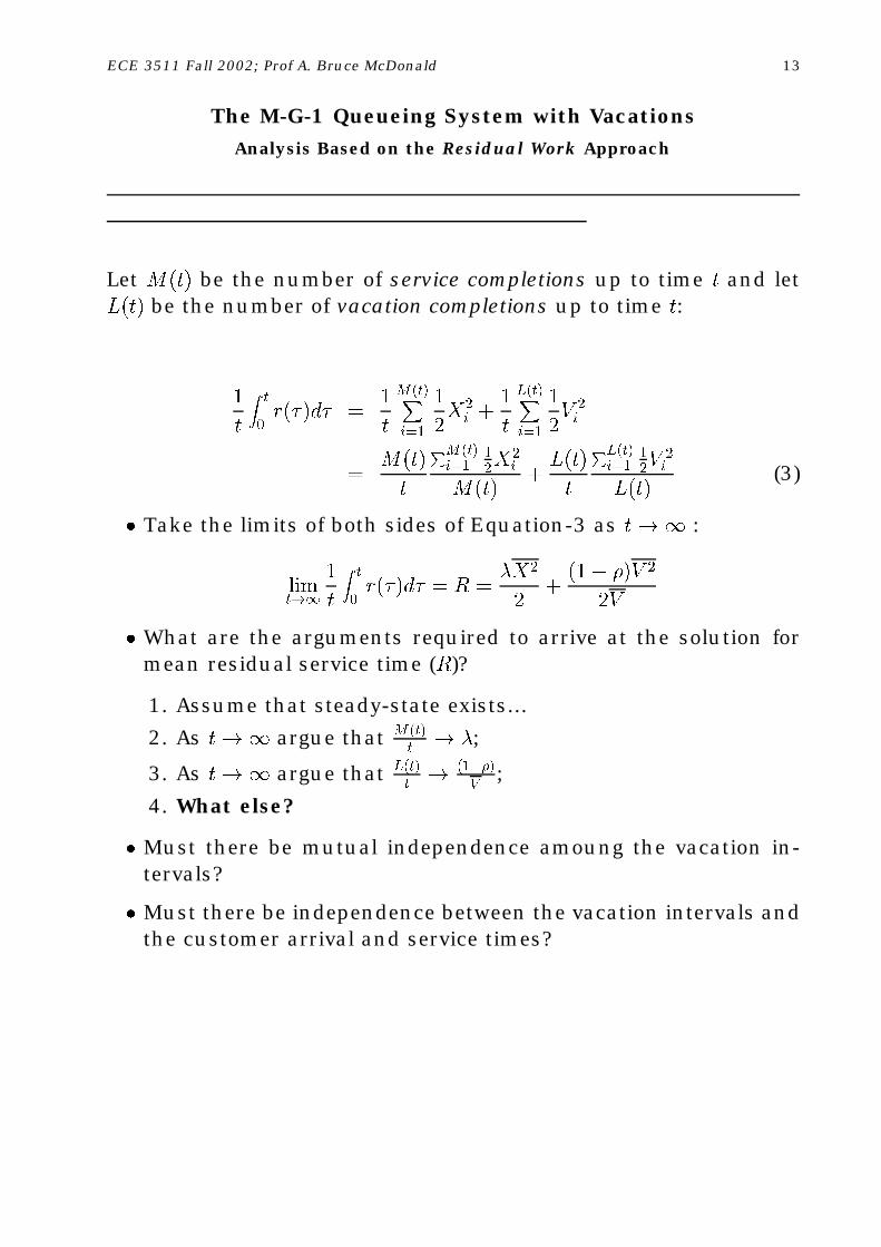
Let M(t) be the number of service completions up to time t and letL(t) be the number of vacation completions up to time t:

1

t

Z t

0r(�)d� =

1

t

M(t)Xi=1

1

2X2

i +1

t

L(t)Xi=1

1

2V 2i

=M(t)

t

PM(t)i=1

12X

2i

M(t)+L(t)

t

PL(t)i=1

12V

2i

L(t)(3)

� Take the limits of both sides of Equation-3 as t!1 :

limt!1

1

t

Z t

0r(�)d� = R =

�X2

2+

(1� �)V 2

2V

� What are the arguments required to arrive at the solution formean residual service time (R)?

1. Assume that steady-state exists...

2. As t!1 argue that M(t)t! �;

3. As t!1 argue that L(t)t! (1��)

V;

4. What else?

� Must there be mutual independence amoung the vacation in-tervals?

� Must there be independence between the vacation intervals andthe customer arrival and service times?

ECE 3511: Communications Networks “Theory and Analysis ...

Documents

Transcript of ECE 3511: Communications Networks “Theory and Analysis ...