EBONEE ALEXIS WALKER Dissertation Submitted to...

INFLUENCE OF PHONON MODES ON THE THERMAL CONDUCTIVITY OF

SINGLE-WALL, DOUBLE-WALL, AND FUNCTIONALIZED

CARBON NANOTUBES

By

EBONEE ALEXIS WALKER

Dissertation

Submitted to the Faculty of the

Graduate School of Vanderbilt University

in partial fulfillment of the requirements

for the degree of

DOCTOR OF PHILOSOPHY

in

Interdisciplinary Materials Science

May, 2012

Nashville, Tennessee

APPROVED:

Professor D. Greg Walker

Professor Richard Mu

Professor Clare M. McCabe

Professor Deyu Li

Professor Keivan G. Stassun

Professor Norman H. Tolk

To Mama Jo—who else?

ii

iii

ACKNOWLEDGEMENTS

Trust in the Lord with all your heart and lean not on your own understanding

—Proverbs 3:5

I thank God and Jesus Christ for my endurance during these last five and a half

years. I do at times wonder how my life would be different if I had moved to Chicago

and become a nuclear reactor inspector, as opposed to taking on an unknown course of

study with little to go on other than my perseverance; but I trust that there is some bigger

purpose in my life that is better served by me having completed this process. I will not

pretend to understand what that purpose may be; but right now, I will take solace in

having conquered every person and contrived task that sought to break my spirit. I am

more than a conqueror.

I say thank you to everyone who offered encouragement. My mother, especially,

gets a big thank you, since she had to listen to my ramblings about carbon nanotubes and

thermal conductivity, as well as my rants about injustices I routinely experienced. My

cheerleading section is my Walker, Cargle, and Cox families, as well as the Mt. Calvary

Baptist Church family; there was never a lack of interest in my progress nor a lack of

encouragement sent out. I have to mention my grandmother, Annie Lee Walker, who

passed away shortly after I began graduate school—though I have learned many things, I

have never forgot what she told me and never found any of it to be untrue.

Of course, graduate school is a long arduous journey and it would be that much

harder if I had to go it alone—but I did not. I want to give my sincere appreciation to

fellow my graduate students. Some that I have known since I showed up back in August

of 2006, like Desmond Campbell, Julia Bodnarik, and Dawit Jowhar—I extend

congratulations to you all. Others—like Lucy Lu and Marquicia Pierce—I came to know

through groups like Toastmasters, GSC, or OBGAPS, because graduate students can have

a life. I cannot say enough about the encouragement I received from those who

completed their studies before me; they never let me get down or believe I would do

anything other succeed, so thanks go to Paula Hemphill, Wole Amusan, Jonathan Hunter,

Saad Hasan, and Lidell Evans. I have to give a really special thanks and congratulations

to John Rigueur, who decided to team up with me to knock our Ph.D.’s out together—

well, we did it Dr. Rigueur! I do not plan to let the gift of encouragement stop with me,

but rather I plan to pass it on not only to other graduate students but to every soul that

needs it.

Not everyone who had an influence on my graduate school experience is a

student. I thank the administrative arms of both Vanderbilt and Fisk Universities. I had

very few problems and that just gave me more time to focus on the main task, so thanks

to the front offices of Mechanical Engineering and Materials Science. I even want to

thank the staff of WFSK for always being encouraging and especially for providing gifts

of entertainment. Though I never applied, I appreciated the Bridge Program for

absorbing me; because the students they accepted were definitely on a track parallel to

mine, and I am glad I had their camaraderie.

For the technical acknowledgements, this research was conducted while affiliated

with the Thermal Engineering Lab. Funding was provided for me by the National

Science Foundation Integrative Graduate Education and Research Traineeship and the

iv

Department of Defense (DoD) Science, Mathematics, and Research for Transformation

fellowship. Computational resources were provided by the Air Force Research

Laboratory DoD Supercomputing Resource Center and ACCRE at Vanderbilt.

v

TABLE OF CONTENTS

Page

ACKNOWLEDGEMENTS............................................................................................... iii

LIST OF TABLES........................................................................................................... viii

LIST OF FIGURES ........................................................................................................... ix

Chapter

I. INTRODUCTION ........................................................................................................ 1

Conduction in Bulk Materials.............................................................................. 2 Conduction in Nanostructures.............................................................................. 6 Carbon Nanotubes................................................................................................ 7

II. LITERATURE REVIEW ........................................................................................... 10

Thermal Conductivity of Individual Carbon Nanotubes ................................... 10 Thermal Conductivity in Double-Wall Carbon Nanotubes ............................... 17 Thermal Conductivity of Functionalized Carbon Nanotubes ............................ 17 Thermal Conductivity in Graphene ................................................................... 22

III. MOLECULAR DYNAMICS ..................................................................................... 24

Newtonian Equations of Motion........................................................................ 24 Interatomic Potentials ........................................................................................ 26 Molecular Dynamics Simulation Methods ........................................................ 29

IV. SIMULATION METHODS ....................................................................................... 31

Models of Carbon Nanotubes ............................................................................ 31 Nonequilibrium Molecular Dynamics Simulation Parameters .......................... 35

Muller-Plathe Method............................................................................ 35 Heat Bath Method.................................................................................. 37

Validation........................................................................................................... 38

vi

V. RESULTS AND DISCUSSION................................................................................. 41

Carbon nanotube thermal conductivity.............................................................. 41 Thermal conductivity of functionalized carbon nanotubes................................ 49 Thermal Conductivity in Graphene ................................................................... 54

VI. CONCLUSIONS......................................................................................................... 57

Future Work ....................................................................................................... 59

A. SIMULATION SCRIPTS..................................................................................... 60

TubeGen Script ............................................................................................... 60 LAMMPS script.............................................................................................. 60

Script for Single-wall Carbon Nanotube Thermal Conductance .............. 60 Script for Double-wall Carbon Nanotube Thermal Conductance............. 63 Script for Double-wall Carbon Nanotube with Interior Wall Heated....... 65 Script for Double-wall Carbon Nanotube with Interior Wall Heated....... 67 Script for Double-wall Carbon Nanotube with Exterior Wall Moving .... 69 Script for Double-wall Carbon Nanotube with Interior Wall Moving ..... 71 Script for Functionalized Single-wall Carbon Nanotube.......................... 73 Script for Functionalized Double-wall Carbon Nanotube ........................ 75 Script for Graphene Thermal Conductance .............................................. 77 Script for Bilayer Graphene Thermal Conductance.................................. 79

B. RAW THERMAL CONDUCTIVITY DATA...................................................... 81

REFERENCES ................................................................................................................. 86

vii

LIST OF TABLES

Table Page

1. Thermal conductivities of CNT samples ................................................................. 11

2. Thermal conductivity of CNTs in Composite Applications .................................... 18

3. Room Temperature Thermal Conductivity in Graphene ......................................... 23

4. Characteristics of CNTs studied. ............................................................................. 32

5. Number of Functionalization Atoms for CNTs ....................................................... 34

6. Mean-square Vibrational amplitudes for 25 nm CNTs with Various Combinations of Vibrational Modes [Longitudinal (L), Radial breathing (B), Torsional (T), and/or Flexural (F)] .......................................................................... 47

7. Mean-square Vibrational amplitudes for 200 nm functionalized SWNTs with Various Functalization Densities ............................................................................. 52

8. Mean-square Vibrational amplitudes for 200 nm 1% functionalized SWNT with Various σ Values ..................................................................................................... 53

9. Thermal Conductivity of CNTs ............................................................................... 81

10. Thermal Conductivity of DWNTs Using Different Heating Schemes .................... 82

11. Thermal Conductivity of CNTs with One Mode Suppressed.................................. 82

12. Thermal Conductivity of CNTs with Two or More Modes Suppressed.................. 83

13. Thermal Conductivity of Functionalized CNTs at Various Percentages................. 83

14. Thermal Conductivity of Functionalized SWNTs for Various Values of the Lennard-Jones Parameter σ ..................................................................................... 84

15. Thermal Conductivity of Graphene with Three and Two Vibrational Modes Present...................................................................................................................... 84

16. Thermal Conductivity of Graphene with One Vibrational Mode Present ............... 85

viii

LIST OF FIGURES

Figure Page

1. Methods of heat transfer [2]....................................................................................... 2

2. A nonequilibrium state exists when a system is in contact with two reservoirs of temperatures T1 and T2 [3]......................................................................................... 3

3. The translational modes in CNTs are shown (a) longitudinal, (b) radial breathing, and (c) flexural........................................................................................................... 5

4. Starting from a graphene sheet armchair, chiral, or zig-zag CNTs can be formed based on the direction of the chiral vector [11]. Armchair SWNT orientation occurs when rolling the graphene sheet from left to right and zig-zag SWNT, when rolling from top to bottom; chiral SWNTs result when the sheet is rolled along any vector in between the armchair and zig-zag direction............................... 8

5. An example of a disconnected CNT generated by TubeGen when the gutter size is not adequate.......................................................................................................... 32

6. A chirality (10,10) CNT generated by the TubeGen coordinate generator. ............ 33

7. A typical (10,10)@(19,10) DWNT.......................................................................... 33

8. A phenyl group. ....................................................................................................... 34

9. A representation of the setup for Muller-Plathe NEMD method in LAMMPS....... 36

10. A typical temperature profile generated by the Muller-Plathe NEMD method....... 36

11. A representation of the setup for constant energy flux NEMD method in LAMMPS................................................................................................................. 37

12. A typical temperature profile generated by the constant energy flux NEMD method...................................................................................................................... 38

13. Comparison of thermal conductivity versus length results for a (10,10) SWNT by the LAMMPS simulator to Padgett and Brenner’s 2004 study. .............................. 40

14. Thermal conductivity of (10,10) and (19,10) SWNTs and a (10,10)@(19,10) DWWNT for lengths from 25 nm to 1 μm. Also shown are the NEMD thermal conductivity of (10,10) SWNTs from other works [12], [28], [29]. ........................ 42

ix

x

15. Thermal conductivity versus length plotted on a log-log scale for a (a) (10,10) SWNT and (b) (19,10) SWNT. The line is thermal conductivity λ ~ Lβ................ 43

16. Thermal conductivity of DWNT using various heating schemes............................ 45

17. Thermal conductivity is shown for the CNT when combinations of modes are restricted [70]. .......................................................................................................... 48

18. Thermal conductivity of a (10,10) SWNT and (10,10)@(19,10) DWNT at different functionalization densities of a phenyl united atom.................................. 50

19. Thermal conductivity of (10,10) SWNT when the functionalizing atoms are mobile and fixed. ..................................................................................................... 51

20. Thermal conductivity of (10,10) SWNT as the Lennard-Jones parameter σ is varied........................................................................................................................ 52

21. Thermal conductivity of graphene that is confined in various directions................ 56

CHAPTER I

INTRODUCTION

The rediscovery of carbon nanotubes (CNTs) by Iijima unveiled a material that

offers promise in many areas of composite engineering [1]. Carbon nanotubes are shown

to have exceptional mechanical, electrical, and thermal properties. Though their high

room temperature thermal conductivity suggests that their inclusion in composite

materials should yield a better thermally conducting composite, experimental studies

have shown inconsistent thermal enhancement at best. Studies that have focused on

incorporating CNTs in composites to enhanced thermal properties have studied the

changes in the thermal conductivity of the matrix material—usually a polymer; few

studies focus on the changes in the CNT’s thermal conductivity when added to the

matrix. By understanding the behavior of the individual CNT, better techniques can be

developed to engineer composites with the desired properties.

Molecular dynamics (MD) simulations offer a technique to understand the atomic

behavior of the CNT and between the CNT and the matrix material. Using MD

simulations, thermal conductivity of the CNT can be studied to identify the contribution

of individual phonon modes and how the modes are affected by interaction with the

surrounding material. Insight can be obtained about how thermal conduction occurs in

the CNT when incorporated into different configurations with the matrix material. This

study will show that not all phonon modes contribute to increasing thermal transport, but

rather their presence may actually produce more scattering.

1

Conduction in Bulk Materials

The nanoscale size of CNTs makes them materials that are unique from their bulk

material counterpart. Often nanostructure’s properties differ from those of the bulk

material due to the effect of their small size. Size effects can cause a material to have

“super” mechanical, electrical, chemical, or thermal properties when compared to the

bulk material. This is often the result of having a larger aspect ratio, larger surface area,

or small characteristic length. When considering heat transport in CNTs, a comparison to

heat transport in bulk carbon materials illustrates the superior performance of the CNT.

Three mechanisms by which heat can be transferred include: conduction,

convection, and radiation. Heat transfer by conduction occurs through a material due to a

temperature difference, convection happens when fluid flow carries heat, and radiation

carries heat by electromagnetic waves (Figure 1). Only the former process is considered

Figure 1 Methods of heat transfer [2]

2

in the scope of this work. Heat conduction occurs when thermal energy is transported by

the random motion of heat carriers, which causes a temperature gradient to form in a

material. The temperature gradient is the driving force that transports energy in the

system; however, this is only true when the system is in a nonequilibrium steady state

(Figure 2). If reservoir 2 has a higher temperature than reservoir 1, then thermal energy

Figure 2 A nonequilibrium state exists when a system is in contact with two reservoirs of

temperatures T1 and T2 [3] will flow through the system from reservoir 2 to reservoir 1 in order to establish

equilibrium; however, if the reservoirs are large their temperatures will be maintained

and a temperature gradient occurs in the system. The steady state characteristic arises

from the heat flux not changing with time. Heat conduction can be described by

Fourier’s law that states the heat flux is proportional to the temperature gradient

Tk∇−=q (1.1)

where q is the local heat flux, k is thermal conductivity, ∇ is the gradient operator such

that the temperature gradient is defined

zyx )))

zT

yT

xTT

∂∂

+∂∂

+∂∂

≡∇ (1.2)

where x) , y) , and z) are unit vectors [5]. The negative sign arises from the energy flowing

down the temperature gradient [6]. Thermal conductivity is a material dependent

Reservoir 1 Reservoir 2 T2

System T1

Energy flow

3

property that measures the effectiveness in conducting heat. Thermal conductivity is

dependent on the direction of the material; therefore, it can be written as a tensor.

Solid materials can have thermal energy carried by phonons, as well as electrons.

Phonons are atomic lattice vibrations. Depending on the material either phonons or

electrons will dominate as heat carriers. For example, in metals electronic contribution is

dominant at all temperatures; however, for semiconductors the mean free path (MFP) of

electrons can be reduced by the presence of impurities, which allows phonons to increase

their contribution to the heat current. Finally, insulators will have phonons as the

dominate heat carriers [7]. Carbon materials’ thermal conductivity tends to be dominated

by phonons due to sp3 and sp2 covalent bonding, which facilitates phonon travel over the

stiff bonds. Each phonon has a specific wavelength. In CNTs the wavelength of the

phonon has a major influence on the amount of thermal energy transported, since the

amount of energy transported increases as longer wavelengths can be included;

consequently, the wavelengths can be shortened due to the presence of scattering events

like defects, impurities, and functionalizing groups.

Furthermore, acoustical phonons carry the majority of heat in materials. Phonons

modes can be described by polarization and branch. Typically, there are three

polarizations: one longitudinal and two transverse. The number of branches depends on

the number of basis atoms in the unit cell; but the branches are categorized as acoustical

or optical. One acoustical branch exists for each polarization and the remaining branches

are optical branches. In CNTs there exist four polarizations: three are translational and

one is rotational. The translational modes are longitudinal (L), radial breathing (B), and

4

Figure 3. The translational modes in CNTs are shown (a) longitudinal, (b) radial breathing, and (c) flexural.

flexural (F). Figure 3 depicts the translational modes in a CNT. The longitudinal modes

displace atoms parallel to the CNT’s axis. Radial breathing modes expand and contract

around the CNT’s axis. Flexural modes displace atoms normal to the axis. The torsional

(T) mode twists in the direction of CNT’s chiral vector. Thermal energy transported in a

material is the combination of energy transported by all the phonon branches for each

polarization.

Thermal conductivity due to the phonons of a material can be written

lCk ν31

= (1.1)

where C is the specific heat, v is the group velocity, and l is the phonon MFP [7].

Specific heat is a measure of the heat required to change a certain mass of the material by

a specified temperature or, alternatively, the heat capacity Cv per unit mass where

Vv

UC ⎟⎠⎞

⎜⎝⎛∂∂

≡τ

(1.2)

for a constant volume [3], where the fundamental temperature τ=kBT and the internal

energy U of the system can be written

5

( ) ( )dEEDEfEU ∫= (1.3)

where E is energy; f(E) is the Bose-Einstein distribution function

1exp

1)(−⎟

⎠⎞

⎜⎝⎛ −

=

τμE

Ef (1.4)

where μ is the chemical potential; and D(E) is the density of states. The group velocity

specifies the direction and speed at which a wave of energy propagates. The phonon

MFP is the avearge distance a phonon will travel before scattering. The MFP can be

written as function of the scattering time t (usually denoted τ)

νtl = ; (1.5)

therefore, a larger average MFP results from a larger scattering time, since scattering

events occur less frequently. Scattering events can be caused by scattering due to other

phonons, impurities, defects, and/or electrons [8]. In bulk carbon materials the MFP will

be much smaller than the size of the material; however, the size of a CNT is comparable

to the MFP. Since the MFP is a larger influence than the specific heat or group velocity,

events that influence the MFP will play a larger role in the thermal conductivity. The

average length of the MFP in CNTs can be decreased by the presence of functionalizing

groups. Also, the interaction between phonon modes can cause the MFP to be shorter

than what might be observed by with a single phonon mode.

Conduction in Nanostructures

Thermal transport can be described as diffusive or ballistic. Diffusive thermal

transport occurs when phonons scatter while traveling through the system; on the other

hand, ballistic transport has no internal scattering events [4]. These transport phenomena

6

can be related to the MFP—the average distance travelled before a scattering event

occurs. When the size of the system is larger than the MFP, scattering events will occur

causing diffusive transport. In ballistic transport, the MFP is larger than the system size;

therefore, no scattering of the phonon can happen before the end of the system is reached.

Fourier’s law is based on the presence of a temperature gradient—and consequently,

diffusive transport. In the case of ballistic transport, a temperature difference, rather than

gradient, exists between the ends of the system [7]. When ballistic transport occurs, the

only scattering event in nanostructures stems from the boundary of the system. Thermal

conductivity scales with the system size; in the ballistic regime, increasing the system’s

size allows phonons of longer wavelengths to contribute to thermal transport and increase

conductivity. If a crystal lattice is perfect, then thermal conductivity is intrinsic and

limited by the anharmonicity of the interatomic forces. The intrinsic scattering processes

can be normal (N) or Umklapp (U) processes. When phonons are scattered by N-

processes momentum is conserved; however, U-processes do not conserve momentum

and are responsible for thermal resistivity. Extrinsic thermal conductivity is limited by

phonons scattering on defects in the crystal [7], [9]. The scope of this study will

investigate the ballistic regime of CNTs at lengths up to 1 μm. Additionally, the effect of

functionalizing atoms and bond strength on the MFP will be studied.

Carbon Nanotubes

Carbon nanotubes (CNTs) are rolled up sheets of graphite that are confined in two

dimensions. If only a single layer of graphite—known as graphene—is used to construct

a CNT, then it is called a single-walled CNT (SWNT); several graphene sheets rolled up

7

to make concentric cylinders are known as a multiwalled CNT (MWNT). A SWNT can

be named according to the direction the graphene sheet is rolled. Figure 4 shows how

CNTs can be rolled up from a graphene sheet and are different based on the direction.

The chiral vector that defines the CNT is

21 mana +=c (1.8)

where a1 and a2 are the basis vectors of the hexagonal graphene sheet [10]. The integers

n and m are used to characterize SWNTs, which are called armchair (n,n), zig-zag (n,0),

or chiral (n,m). Armchair SWNTs have electrical properties that are metallic. Zig-zag

Figure 4 Starting from a graphene sheet armchair, chiral, or zig-zag CNTs can be formed based on the direction of the chiral vector [11]. Armchair SWNT orientation occurs

when rolling the graphene sheet from left to right and zig-zag SWNT, when rolling from top to bottom; chiral SWNTs result when the sheet is rolled along any vector in between

the armchair and zig-zag direction. and chiral SWNTs are metallic if (n-m)/3; otherwise, they are semiconducting where the

bandgap is inversely dependent on the diameter of the tube [11].

8

Like other carbon allotropes, CNTs exhibit exceptional thermal properties. The

strong carbon bonds are paramount to the transport of thermal energy. The bonds

between carbon atoms are strong and stiff, which is ideal for achieving high thermal

conductivity. For CNTs thermal conductivity along the axis is very large. For MWNTs,

thermal conductivity in the radial direction is expected to be lower; the decrease comes

from the additional effect of weak van der Waals forces between the layers of the

MWNT. The thermal conductivity of CNTs is generally independent of the chirality of

the nanotube [12]. The length of the CNT plays a large role in the thermal conductivity

in the longitudinal direction. As the length of the CNT increases, the thermal

conductivity will increase as the length approaches the CNT’s MFP—as the CNT

becomes longer, more phonon wavelengths can participate in the thermal transport. The

diameter of the CNT is related to the chirality, because larger chiralities typically lead to

larger diameters; although, the larger diameter leads to increased conductance the thermal

conductivity will remain independent of that fact.

9

CHAPTER II

LITERATURE REVIEW

Thermal Conductivity of Individual Carbon Nanotubes

Carbon nanotubes have shown a range of thermal conductivity values at room

temperature (Table 1). Early experiments used samples of CNT mats, which would show

a lower thermal conductivity than an individual CNT due to the interaction between the

multiple CNTs [13–15]. Experiments on SWNT mats showed a thermal conductivity of

35 W/m/K at room temperature when corrected for the sample’s low density [13].

Measurements of MWNT films had a thermal conductivity of 15 W/m/K; the MWNTs

were estimated to have a thermal conductivity of 200 W/m/K when corrected for volume

[14]. Hone et al. measured thermal conductivity parallel to the axis of a SWNT mat to

have a thermal conductivity of ~225 W/m/K [15]. Using measurement devices that

suspend the CNT, thermal conductance was measured for individual CNTs and thermal

conductivity estimates were consistently shown to be well over 1000 W/m/K. Kim et al.

determined thermal conductivity for an individual MWNT with a diameter of 14 nm was

~3000 W/m/K [16]. A thermal conductivity of ~2000 W/m/K was measured by Fujii et

al. using a CNT with a diameter of 9.8 nm [17]. Thermal conductivity was shown to

increase with decreasing diameter. Thermal conductivity for SWNT was measured as

3000 W/m/K for a 3 nm diameter by Yu et al. [18]. Single-walled CNTs were measured

to have 3500 W/m/K by Pop et al. [19]. Small et al. measured thermal conductivity of

MWNT on a microfabricted suspended device to be >3000 W/m/K [20]. When using the

10

Table 1 Thermal conductivities of CNT samples Sample Length (nm) Measurement

Method Thermal

conductivity at 300 K

(W/m/K)

Reference

SWNT mat 2x106 Comparative: constantan rod

0.7 (35 corrected for

density)

[13], [23]

(10,10) SWNT 1 Equilibrium MD

6600 [25]

(10,10) SWNT <50 Equilibrium MD

2980 [26]

Magnetically aligned bulk SWNT

5x103 Comparative: constantan rod

~225 [15]

MWNT 2.5x103 Microfabricated suspended

device

~3000 [16], [27]

(10,10) SWNT 15.1 - 21.1 NEMD ~1500 [12] MWNT films 10 - 50x103 Pulsed

photothermal reflectance

~15 (200 corrected for

volume)

[14]

(10,10) SWNT ~400 NEMD ~300 [28] MWNT 2x106 Microfabricated

suspended device

>3000 [20]

(10,10) SWNT <50 Homogenous nonequilbirum Green-Kubo

~2000 [29]

(5,5) SWNT 10.8 NEMD 800 [30] Individual CNT 3.7x103 Sample-

attached T-type nanosensor

>2000 [17]

SWNT 2.76x103 Microfabricated suspended

device

3000 [18]

MWNT ~1x103 2-point 3ω 830 [21] (10,10) SWNT ~40 Equilibirum

MD: Green-Kubo

~1635 [31]

SWNT 2.6x103 Direct self-heating

3500 [19]

MWNT 1.4x103 4-point 3ω 300 [22]

11

3ω method, Choi et al. found one MWNT sample to have 830 W/m/K [21]. Thermal

conductivity of 300 W/m/K for a MWNT was measured by four-point 3ω method [22].

Using a four pad setup in the 3ω method improves the accuracy of the measurement,

because contact resistance can be eliminated. The lower measurement by Choi et al.

when using the improved technique most probably arises from the samples, since the

two-point 3ω method used a MWNT with a diameter ~40 nm and the four-point 3ω

method used a MWNT with a diameter ~20 nm. All the measurements have CNTs that

are at least several microns long, yet thermal conductivities at room temperature are

exceptionally large. This result is an indication that the phonon MFP is quite large for

CNTs.

Measuring the thermal conductivity of individual CNTs has received much

attention over the last decade. Initially, a comparative method using a constantan rod was

used to measure bulk SWNT samples [13], [15], [23], [24]. Temperatures from 8-350 K

were used by Hone et al. to measure SWNT mats. Later Hone et al. measured the

thermal conductivity of aligned SWNT mats. Llaguno et al. measured thermal

conductivity for bulk SWNTs from 10-100 K. Another technique used to measure bulk

samples, the pulsed photothermal reflectance technique, was used by Yang et al. to

measure thermal conductivity in MWNT films [14]. The development of suspended

microfabricated devices has made possible measuring thermal transport in a single CNT

free from substrate influence [16], [18], [19]. A microfabricated suspended heater device

is used to measure thermal conductance from 8-370 K of an individual MWNT and from

100-300 K for a SWNT [16], [18], [20]. Using a sample-attached T-type nanosensor,

Fujii et al. measured temperature dependence from 100-320 K, as well as diameter

12

dependence [17]. Another temperature dependent study of SWNTs employs direct self-

heating for 300-800 K. Choi et al. used the 3ω method to measure thermal conductivity

on individual MWNTs [21]. Using a four-point 3ω method, Choi et al. calculate thermal

conductivity for an individual MWNT [22]. Length-dependent thermal conductivity was

measured for an individual SWNT using a four-pad 3ω method [32].

The thermal conductivity of a CNT is estimated because only thermal

conductance can be determined from an experiment or simulation. Kim et al. measured

the thermal conductance of a MWNT and estimated a thermal conductivity of

approximately 3000 W/m/K at 300 K [16]. In 2005 Yu et al. measured a SWNT’s

thermal conductance and estimated the room temperature thermal conductivity could

range from 3000 W/m/K if the SWNT’s diameter is 1 nm to 10000 W/m/K if the

diameter is 3 nm [18]. Each of these studies measure thermal conductance rather than

thermal conductivity; therefore, thermal conductivity is based on an estimation of the

CNT’s cross-sectional area. The area of a CNT, however, is ambiguous since its cross-

sectional area is a ring with the thickness of a carbon atom. Hone et al. used a cross-

sectional area of a tube in a bundle as 2.5 nm2. A 1 Å thick cylinder was used by Che et

al. [26]. A ring with thickness 3.4 Å is the van der Waals thickness [12], [28]; in

contrast, Zhang and Li used a ring thickness of 1.44 Å [30]. The result of using different

cross-section areas is yielding different estimates for thermal conductivity. A large cross-

sectional area, such as a circle, will yield a smaller thermal conductivity than a smaller

cross-sectional area estimate, like a ring. The influence on the thermal conductivity

results, however, is minimal if the same cross-sectional area is used for all data

considered. Needless to say when comparing thermal conductivity estimates from

13

multiple studies the cross-sectional area used by the investigators must be taken into

consideration, since it will give an idea if the value is a high or low estimate.

The thermal conductivity of CNTs exhibits temperature dependence. At 100 K,

thermal conductivities of SWNTs could be as high as 37000 W/m/K [25]. Thermal

conductivity increases with increasing temperature to a peak around 300 K [17]. Pop et

al. measured SWNTs for high temperatures (300-800 K) and found thermal conductivity

decreases as temperatures rise above 300 K; they estimated a value of almost 1000

W/m/K for 800 K [19]. Similarly, each study reported the maximum thermal

conductivity at room temperature after which the thermal conductivity declines. Also,

each study reported similar room temperature thermal conductivities for both SWNT and

MWNT; the diameters of the SWNTs were approximately 1-2 nm and the diameter for

the MWNT was about 14 nm.

The thermal conductivities of CNTs can be influenced by several factors. The

temperature dependence of thermal conductivity is affected by the heat capacity and

phonon MFP—at low temperatures the MFP is long and thermal conductivity follows the

heat capacity; but at higher temperatures, where the heat capacity becomes constant,

thermal conductivity is governed by the umklapp scattering processes, which shorten the

MFP and decreases thermal conductivity [25]. Specifically, the MFP is made up of the

static MFP and umklapp MFP where at low temperatures the MFP equals the static MFP

and as the temperature increases the umklapp MFP increases and thermal conductivity

decreases [16]. The high thermal conductivity observed when measuring individual

CNTs can be influenced by the lost of heat to the surroundings, which cause an

overestimation of thermal conductivity [14]. Multiwalled CNTs may exhibit lower

14

thermal conductivities due to interaction between the tubes and, in the case of

experiments, the presence of defects within the CNTs. The chirality can also cause

differences in thermal conductivities of CNTs that have the same diameter. As the

chirality decreases, the strain on the sigma bonds reduces the MFP of the CNT [12], [29];

however, Zhang and Li concluded thermal conductivity in CNTs is insensitive to

chirality—they did not consider CNTs that were of equal radii, but different chiralities

[30]. Cao et al. studied the affect of chirality in zigzag SWNTs—they showed that small

diameters had higher conductivities and there was a peak temperature after which thermal

conductivity would decrease [33], [34].

Molecular dynamics simulations have seen extensive use in the simulation of

SWNTs’ thermal conductivity [12], [25], [26], [31]. Simulations types include NEMD

methods using heat baths, as well as equilibrium MD methods based on the Green-Kubo

expression. Another simulation is the homogenous nonequilibrium Green-Kubo

(HNEGK) method employed by Zhang et al. [29]

Similar to studies of experimental measurements of CNTs, theoretical studies

have produced large thermal conductivity predictions. Using NEMD, Berber et al.

estimated a room temperature thermal conductivity of 6600 W/m/K [25]. Che et al. used

equilibrium MD, to estimate a thermal conductivity of 2980 W/m/K [26]. Thermal

conductivity for (5,5) SWNT was estimated to be ~2250 W/m/K and ~1500 W/m/K for

(10,10) SWNT by Osman and Srivstava [12]. The room temperature estimation by

Maruyama averaged 300 W/m/K for (10,10) SWNTs and appeared to be independent of

length [28]. The (5,5) SWNT studied reached a thermal conductivity of ~490 W/m/K at

~200nm. The simulation of Zhang et al. showed a (10,10) SWNT thermal conductivity

15

of ~2200 W/m/K [29]. Using equilibrium MD with the Green-Kubo formulation,

Grujicic et al. estimated thermal conductivity to be ~1635 W/m/K [31]. The variations

can be attributed to the use of different size simulations—with some systems containing

only 400 atoms and others up to 6400 [25], [26].

Studies for length-dependent thermal conductivity have been conducted for

CNTs. Many theoretical studies have shown thermal conductivity to converge at short

lengths. Using lengths <50 nm, Che et al. show that thermal conductivity of a (10,10)

SWNT converges to 2980 W/m/K [26]. Padgett and Brenner found thermal conductivity

converged at <300 nm at a thermal conductivity of ~350 W/m/K [35]. Grujicic et al.

found thermal conductivity converges for the (10,10) SWNT at a length of ~40 nm [31].

The convergence of the thermal conductivity implies that thermal transport has

transitioned from purely ballistic to diffusive; however, other studies show thermal

conductivity growing rapidly as length increases. For lengths up to 200 nm, Maruyama

used NEMD simulations to show (5,5) SWNTs had a divergent thermal conductivity as

length increases, but (10,10) SWNTs thermal conductivity was essentially non-divergent

[28]. Thermal conductivity of SWNT’s divergence is ~Lβ as length L increases [28],

[30]. The divergence of thermal conductivity with length was studied by Zhang and Li

who found the divergence power parameter β decreases with an increasing CNT radius

and also with increasing temperature indicating less divergence with increases scattering

[30]. Maruyama speculated the limited motion of smaller radius CNTs contribute to the

divergence [28]. Though length-dependent measurements of individual CNTs tends to be

cumbersome, some experimental investigations have been conducted to explore the

length-dependent behavior of CNTs. Yang et al. measured MWNT films using pulsed

16

photothermal reflectance and found the thermal conductivity of the films to be

independent of the length of the MWNTs [14]. A length-dependent experiment was

performed by Wang et al. using a four-pad 3ω method to measure thermal conductivity

from 0.5-7 μm [32]. Thermal conductivity multiplied by the tube diameter was shown to

increase with thermal conductivity before appearing to converge. The difference in the

length scales between the theoretical and experimental studies suggests the short length

simulations do not fully describe the thermal conductivity behavior of the CNTs.

Thermal Conductivity in Double-Wall Carbon Nanotubes No MD simulations studies of thermal conductivity of DWNTs have been

identified in the literature at this point in time. Of the DWNT MD simulations that do

exist, the structural and mechanical properties of the DWNTs are the focus of the study.

Saito et al. studied DWNTs to determine optimum geometries for various inner and outer

diameters [36]. They concluded the minimum energy geometry depends on the interwall

distance, a conclusion found by others as well [37]. Some MD simulations focus on the

reaction of structures in the presence of other molecules [38]. Molecular dynamics

simulations are used to estimate mechanical properties like Young’s modulus of DWNTs

[39]. An MD simulation of the length-dependent thermal conductivity of DWNTs will be

a major contribution to theoretical studies of CNTs.

Thermal Conductivity of Functionalized Carbon Nanotubes

Using CNTs in composite materials to improve thermal properties have been

studied in many aspects. Carbon nanotubes have a large aspect ratio and thermal

17

conductivity of 3000 W/m/K at 300 K. These advantageous properties make CNTs

desirable filler for composite materials. Impediments to achieving the desired thermally-

enhanced composite material exists due to resistance at the interface of the CNT and

matrix material and the difficulty of enhancing mechanical and thermal properties

simultaneously. The studies using CNTs as thermal enhancers are inconsistent in

demonstrating an improved composite material (Table 2).

Table 2 Thermal conductivity of CNTs in Composite Applications Sample Loading Method RT Thermal

conductivity (W/m/K)

Reference

MWNT in poly (α-olefin) oil

1 vol% Transient hot wire

0.3765 [40]

SWNT-epoxy composite

1 wt% Comparative: constantan rods

~0.5 [41]

Nitric acid treated MWNT in decene

1 vol% Transient hot wire

0.1674 [42]

(5,5) SWNT Up to 50% 14C isotope

impurities

NEMD ~350 [30]

(10,10) SWNT 10% functionalized with phenyl

groups

NEMD ~25 [35]

Carbon nanotubes have produced enhancements to the thermal conductivity of the

matrix material but not to the full potential of predicted CNT thermal conductivity.

Though Choi et al. show a 160% enhancement in their nanotube-in-oil suspension with

only 1 vol% of MWNTs added, the thermal conductivity of the oil is enhanced from

0.1448 W/m/K to 0.3765 W/m/K [40]. Acoustic impedance mismatch at the interface of

the liquid and solid prevents larger enhancement [40]. The results the treated MWNTs of

Xie et al. do not demonstrate increased enhancement, but rather produces less

enhancement. Similar results are shown in composites, Biercuk et al. showed an increase

18

in thermal conductivity of the epoxy resin from ~0.2 W/m/K at 300 K to ~0.5 W/m/K

[41].

Suspensions were the first systems to provide insight on thermal conductivity

with CNT fillers. Choi et al. produced a nanotube-in-oil suspension using MWNTs and

found the effective thermal conductivity of the oil increased with a small volume fraction

of MWNTs [40]. They measured enhancement of the oil (160%) greater than any

enhancement predicted by theoretical models of solid/liquid suspensions (10%).

Suspensions of pristine and treated MWNTs in distilled water, ethylene glycol, and

decene were measured by Xie et al. [42]. The surfaces on the MWNTs were treated with

nitric acid. For the treated MWNTs, they demonstrated enhancements of 7%, 12.7%, and

19.6% for distilled water, ethylene glycol, and decene, respectively. Biercuk et al.

measured a 125% enhancement with 1 wt% of SWNTs added to an epoxy resin. Thermal

conductivity enhancement is attributed to ballistic heat conduction and to the large aspect

ratio [40], [41]. When nanotubes are surface treated, thermal conductivity in suspensions

is governed by matching the frequency of phonons at the interface. For instance high

frequencies in the CNT must be converted to lower frequencies before energy can be

exchanged with the surrounding medium [43].

The success of CNT suspensions were followed by the study of solid CNT-based

composites. Several experimental studies use CNTs to thermally enhance the thermal

properties of epoxy resins. Biercuk et al. studied the thermal enhancement of single-

walled CNTs (SWNTs) in an Epon 862 epoxy resin [41]. With only 1 wt% of SWNTs,

the result was a 125% enhancement relative to the pristine epoxy; however, the thermal

conductivity of the composite was ~0.5 W/m/K, since the pristine epoxy’s thermal

19

conductivity was ~0.2 W/m/K. In addition to SWNTs, Moisala et al. also used

multiwalled CNTs (MWNTs) in their study to enhance bisphenol-A resin [44]. Use of

0.1-0.5 wt% of SWNTs reduced the thermal conductivity of the pristine resin from ~0.25

W/m/K to ~0.23 W/m/K. The MWNTs, on the other hand, increased thermal

conductivity to ~0.29 W/m/K. In both studies the effective thermal conductivity is

below theoretical predictions [45]. Biercuk et al. did not yield any conclusions on what

mechanisms cause the SWNTs to yield a thermal enhancement. The only conclusion

related to thermal conductivity was to mention the large aspect ratio and nanoscale

diameter make SWNTs preferable over carbon fibers, because SWNTs can form an

extensive network at a lower weight percent; however, this attribute is usually more

applicable to electrical conductivity, rather than thermal conductivity because electrons

travel along low resistance pathways whereas phonons travel through atomic vibrations.

Moisala et al. concluded the decrease in thermal conductivity when using SWNTs was

caused by either a large interface resistance due to poor phonon coupling between the

SWNT and the polymer or dampening of the phonons of the SWNTs. In the case of

phonon dampening, the MWNTs could sustain a higher thermal conductivity because the

inner walls could continue to carry phonons. An approach to address both phonon

dampening and interfacial resistance is functionalizing CNTs.

Molecular dynamics simulations were used to investigate the influence of surface

anomalies on the thermal conductivity of SWNTs. Any disturbance in the CNT’s

topology results in a decrease in thermal conductivity. Che et al. completed a study on

the affects of vacancies and defects on the thermal conductivity of a SWNT. Vacancies

were found to cause more degradation in the thermal conductivity than defects; from the

20

simulations, the lowest observed thermal conductivity was 400 W/m/K for a 0.01

vacancy concentration and 1500 W/m/K for a 2.5 defect concentration. Che et al.

concluded that defects preserve the general structure of the SWNT and bonding

characteristics; however, vacancies presented no more of an influence on a one-

dimensional CNT than would have been present on a three-dimensional diamond [26].

Padgett and Brenner extended the study of surface defects’ influence on SWNT’s thermal

conductivity by adding covalently bonded phenyl rings [35]. At ~125 nm, a (10,10)

SWNT with 0.25% of its atoms functionalized with phenyl groups shows a decrease in

thermal conductivity of 100 W/m/K; at 10% functionalization at the same length thermal

conductivity is only ~25 W/m/K [35]. Concluding, the MFP of the phonons was reduced

when only 1% of the CNT’s atom was functionalized and resulted in a decrease of

thermal conductivity by a factor of 3. Studies have shown that thermal conductivity

decreases when CNTs have impurity or functionalizing atoms included. Zhang and Li

used NEMD to simulate the influence 14C isotope impurity has on the thermal

conductivity of (5,5) SWNTs [30]. As the percentage 14C isotopes is increased in the

(5,5) SWNT, thermal conductivity decreases from a maximum of 800 W/m/K when there

are zero impurities to ~300 W/m/K when 50% of the carbon atoms are 14C isotopes.

Additionally, over all temperatures studied a 40% 14C SWNT has thermal conductivity

that is at most 60% of the thermal conductivity of a pristine SWNT. The impurities cause

the phonon-phonon scattering that shortens the MFP of the CNT.

Functionalization of CNTs in experimental studies has shown more consistent

results. Gojny et al. studied nanotube-based composites using SWNTs and

functionalized and unfunctionalized DWNTs and MWNTs [46]. Their results indicate

21

thermal conductivity is dependent on phonon mechanisms, since increasing the CNT

loading improves electrical conductivity—which is based on a percolation mechanism—

but not thermal conductivity. Similar to Biercuk et al., MWNTs outperformed SWNTs;

additionally, DWNTs yielded a higher thermal conductivity as well. When the DWNTs

and MWNTs are functionalized with amino groups, thermal conductivity is lower than

the unfunctionalized CNTs. The conclusion is a weaker interaction between the CNT and

the matrix allows the CNT to transport more efficiently because the coupling is weaker.

Minimizing the coupling between the CNT and matrix reduces phonon dampening in the

CNT, which reduces the CNT’s thermal conductivity. Like previous studies, the

composites’ thermal conductivities are not largely improved over that of the pristine

resin. Understanding the CNT’s response to the matrix interaction is essential to

engineering thermally-enhanced composites.

Thermal Conductivity in Graphene

Graphene, which is an unrolled SWNT, has been measured and found to have

thermal conductivities that are larger than CNTs. Balandin et al. used confocal micro-

Raman spectroscopy to make the first measurement of suspended single-layer graphene

[47]. Similar to experiments with CNTs, the acoustic phonons are found to account for

the majority of the contribution to thermal conductivity. The Klemens’ approximation

was used by Nika et al. to predict thermal conductivity in graphene flakes [48–51]. They

showed that various Gruneisen parameters, a measure of the effect of changing a crystal’s

volume has on vibrational properties [52], influence thermal conductivity in the graphene

flakes of different lengths and temperatures. The long phonon mean free path in

graphene is attributed with the large thermal conductivities, since boundary scattering

22

dominates when the width of graphene is comparable to the mean free path. A similar

result is found by Hu et al. while studying thermal conductivity and rectification in

graphene nanoribbons [53]. Graphene nanoribbons with a zigzag chirality showed higher

thermal conductivities than armchair; symmetrical and defect free graphene nanoribbons

had thermal conductivities higher than the alternative. Different phonon scattering rates

(and by extension mean free paths) yield the various thermal conductivities found in the

different graphene nanoribbon models. Graphene nanorribon thermal conductivity was

found to have sensitivity to edge shape, width, and strain by Guo et al. [54].

Table 3 Room Temperature Thermal Conductivity in Graphene

Sample Length Method Thermal Conductivity (W/m/K)

Reference

Single layer graphene

~3 μm Confocal micro-Raman spectroscopy

5300 [47]

Graphite monolayer

1 nm Equilibrium MD

~6600 [25]

Single layer graphene

1-5 μm Confocal micro-Raman spectroscopy

3080-5150 [55]

Graphene flakes

1-50 μm Klemens approximation [48], [49]

~8500 [50], [51]

Graphene nanoribbons

~5 nm MD ~2000 [53]

Graphene nanoribbons (armchair)

11 nm NEMD 218 [54]

23

CHAPTER III

MOLECULAR DYNAMICS

Molecular dynamics (MD) simulations provide the ability to understand materials

at a length scale where direct measurement is often difficult. Molecular dynamics

simulations are a method of analyzing the behavior of a material at the atomistic scale.

Molecular dynamics simulations are numerical computations of the estimated path of an

atom or molecule. Classical MD simulations are based on Newton’s second law of

motion and an interatomic potential. If the mass and the interatomic potential are known,

then the next position in time can be determined. Results of the calculated trajectory can

be analyzed to determine properties, like thermal conductivity [4].

Newtonian Equations of Motion

The trajectory of an atom is estimated by solving Newton’s second law of motion.

This simple equation becomes a complex computation since each atom’s equation of

motion must be solved. The general Newtonian equation of motion for a system of N

atoms is shown

2

2

1 dtd

m ii

N

ijj

ijr

F =∑≠=

Ni ,...,2,1= (3.1)

where Fij is the force exerted on atom i caused by atom j and mi and ri are the mass and

position of atom i, respectively. A limitation of the Newtonian equation is it requires

additional equations to describe rotational motion [4]. By using the Lagrangian or

24

Hamiltonian equations of motion, all the degrees of freedom of an atom’s trajectory can

be obtained in one vector of generalized coordinates, r. The system’s Lagrangian is

defined as the difference of the kinetic energy and potential energy,

)(),(),,( rrrrr UKtL −= && (3.2)

here is the time derivative of r or the generalized velocity. The Lagrange equation of

motion is

r&

0=∂∂

−⎟⎟⎠

⎞⎜⎜⎝

⎛∂∂

ii

LLdtd

rr& (3.3)

the subscript i denotes the generalized coordinates for each atom. Similarly, the

Hamiltonian describes the energy of the system; however, it describes the total energy of

the system

)()(),,( rppr UKtH += (3.4)

the Hamiltonian is a function of the generalized coordinate vector r and a generalized

momentum p. The generalized momentum is derived from the Lagrangian by

differentiating with respect to the generalized velocity

i

Lr

p&∂∂

= (3.5)

the Hamilton equations of motion are

ii

Hr

p∂∂

−=& i

i dHp

r ∂=& (3.6)

Any of the three equations of motion can be used to describe the atom’s trajectory.

25

Interatomic Potentials

The most crucial aspect of a MD simulation is the interatomic potential. The

interatomic potential describes the forces that act between atoms. In order to produce

reasonable results, the interatomic potential must give an accurate description of the

interaction in the system. The potentials, however, are limited to being only as good as

the data (either from experiments or ab initio simulations) upon which they are based.

Molecular dynamics simulations of atoms have potentials that can be categorized as pair,

many-body, and force fields. The simplest interatomic potential is one describing the

interaction between two atoms—this type of potential is known as a pair potential.

Examples of pair potentials include Coulomb’s, Newton’s law of universal gravitation,

Lennard-Jones, and Morse potentials; the former two are outside the scope of this work.

The Lennard-Jones and Morse potentials are often used in MD simulations.

The Lennard-Jones potential is used in MD simulations to describe non-bonded

interactions. The Lennard-Jones potential is defined

612ijij

ij rA

rBU −= (3.7)

where rij is the distance between two atoms i and j, , and [7], [4].

On the right-hand side, the first term is a repulsive potential, which acts when the two

atoms’ nuclei or inner-shell electrons begin overlapping [4]; the second term is an

attractive potential caused by dipole moments that the atoms induce in one another [7].

The Lennard-Jones potential is useful for describing the interaction of crystals of noble

gases, like argon. In noble gases the interactions are non-bonded, since the outer shells

are completely filled. The forces between the atoms are governed by van der Waals

forces. These are same forces that occur between layers of graphite and the walls of

64εσ=A 124εσ=B

26

CNTs.; therefore, the Lennard-Jones potential is useful in describing the interaction

between the walls of DWNTs and between functionalizing united atoms groups and the

CNT’s exterior, because these are non-bonded interactions. The Lennard-Jones potential,

however, is insufficient to describe the interactions associated with covalent bonds.

In the scope of this work, interatomic potentials that consider the how the

interactions between two atoms are influenced by other atoms are many-body potentials

and forcefields. With carbon systems like graphite, diamond, and nanotubes, the

interaction between two carbon atoms depends not only on the distance between the

atoms, but also on the atoms surrounding the pair. Several potentials exist that describe

the interaction in carbon systems [56]; however, these potentials are largely based on

mechanical properties such as Young’s modulus, rather than thermal properties. Two

many-body potentials that describe the covalent bonding present with structures

containing carbon are the Tersoff potential and the reactive empirical bond-order (REBO)

potential. The Tersoff potential is the first potential that considered bond-order and

allowed for bonds to be formed and broken during the simulation, which is useful in

studying chemical reactions, and it considers the bond angle between atoms i, j, and k

[57], [58]. The form of the Tersoff potential gives the total energy of the system, E,

iji

i VEE21

==∑ (3.8)

where Ei is the site energy and Vij is the bond energy defined as

)]()()[( ijAijijRijijCij rfbrfarfV += (3.9)

the functions fC, fR, and fA represent a smooth cutoff, repulsive pair potential, and an

attractive pair potential, respectively; the function aij consists of range-limiting terms and

bij is a measure of the bond order [58]. The REBO potential is a type of Tersoff potential

27

that is especially good at modeling the interactions in hydrocarbons and graphite [59];

however, the REBO potential is only good for short interactions that are intramolecular.

The REBO potential was extended to include Lennard-Jones terms to account for

intermolecular interactions, as well as torsional interactions [57]. The potential is called

adaptive intermolecular REBO (AIREBO) potential, which is defined

torsLJREBO EEEE ++= (3.10)

where,

)()( ijA

ijijijR

ijREBO rVbrVE += (3.11)

the first term on the right-hand side is the repulsive pair potential and the second,

attractive; the torsional term of Eqn. (2.10) defines the dihedral angle determined by

atoms i, j, k, and l

)()()()( ijkltors

jljlijijkikitorsijkl VrwrwrwE ω= (3.12)

where

kijlkijlkijlkijltorsV εωεω

101)2/(cos

405256)( 10 −= (3.13)

The covalent bonds of CNTs use the Tersoff potential and Lennard-Jones

potentials model the van der Waals forces between the layers of DWNTs and the united

atom models. To study transport properties interatomic potentials that contain

anahrmonicities are needed, thermal conductivity cannot be studied using a harmonic

potential because scattering will not occur.

28

Molecular Dynamics Simulation Methods

Thermal transport properties can be determined by using MD simulations. Two

simulation methods exist for using MD simulations to find thermal information—

nonequilibrium and equilibrium dynamics. A nonequilibrium MD simulation method

(NEMD) can be used to understand thermal transport processes; however, when using an

equilibrium MD (EMD) simulation method only thermal properties can be determined.

A NEMD simulation is typically faster than an EMD simulation, since the EMD

simulation relies on calculation of a computationally expensive autocorrelation function;

however, NEMD simulations can have inconsistencies when defining local thermal

equilibrium, temperature distributions, and boundary conditions in systems with long

mean free paths [4].

Two methods are popular for imposing nonequilibrium conditions on a system.

One method is to impose a temperature gradient and calculate the heat flux—the other

imposes a heat flux and calculates the temperature gradient sometimes called a reverse

NEMD (RNEMD) simulation. Using reservoirs to control the temperature requires a

large temperature difference, but by using the constant heat flux method this issue can be

circumvented [4]. One implementation of a RNEMD simulation is to add and subtract a

heat flux from defined hot and cold regions of the system, respectively. The heat flux is

added (or subtracted) by rescaling the velocity in that region. By adding and subtracting

heat fluxes in the hot and cold regions equally, a temperature gradient is established in

the system. Another RNEMD simulation method introduced by Muller-Plathe, imposes a

constant heat flux by exchanging kinetic energy between the hot and cold regions [60],

[61]. The velocity vector of the hottest atom in the cold region is exchanged with that of

29

the coldest atom in the hot region—the atoms must be of the same mass to conserve

linear momentum. The heat flux is known from the amount of kinetic energy exchanged

during the simulation time of the system; what results for the exchange of energy is a

temperature gradient between the hot and cold regions.

Alternative to the nonequilibrium methods of MD are equilibrium methods.

There is no temperature difference applied to the system in EMD simulation, but rather

the history of the atoms’ movement in the system is used to determine thermal properties.

The Green-Kubo formula can be used to find thermal conductivity directly

( ) ( ) dttTVk

Tk QQB

∫∞

•=0

2 03

1)( JJ (3.14)

where V is the volume of the system, kB is the Boltzmann constant, and JQ is the heat

current [4]. The term in the integral is the heat current autocorrelation function, which is

a time-delayed comparison of the heat current to itself. The EMD simulation tend to be

more computationally expensive than NEMD simulation methods, since the heat current

must be calculated for a many time steps for all the atoms. Since length-dependent

thermal conductivity experiments will be performed, the use of EMD simulations is a less

desirable method than the NEMD simulation methods.

30

CHAPTER IV

SIMULATION METHODS

Molecular dynamics (MD) simulations of CNTs are performed to predict how

thermal transport is affected by non-bonded interactions. Types of CNTs studied include

single-wall CNTs (SWNTs), double-wall CNTs (DWNTs), and functionalized SWNTs

and DWNTs. Using the Tersoff and Lennard-Jones potentials, simulations are performed

using the Large-scale Atomic/Molecular Massively Parallel Simulator (LAMMPS)

distributed by Sandia National Labs [62]. Nonequilibrium MD (NEMD) and wave

packet simulations are used to gather thermal conductivity and thermal transport data.

Models of Carbon Nanotubes

Carbon nanotube coordinates used in the simulation are generated using

TubeGen. TubeGen is able to produce a variety of molecular nanotubes; TubeGen has

the flexibility to generate the coordinates of not only carbon nanotubes, but also other

molecules like boron nitride [63]. Based on the desired chirality, TubeGen yields a

tubular unit cell. Nanotubes with large chiral vectors have unit cells containing more

atoms and larger diameters. To achieve a CNT of the desired length, the unit cell is

replicated along the axial direction (z-axis); the correct number of unit cells to replicate

can be obtained by dividing the length of the CNT by the length of the unit cell (~ 0.1

nm). Table 4 shows the chiralites investigated and their properties; the lengths are

studied for a range of 25 nm to 4 μm.

31

Table 4 Characteristics of CNTs studied. Chirality Diameter (nm) Atoms in Unit Cell

(5,5) 0.7 20 (10,10) 1.4 40 (19,10) 2.0 868 (37,37) 5.0 148 (80,80) 10.9 320

When using TubeGen it is important to set ample gutter spacing to obtain the

correct atom coordinates; otherwise, atoms that are outside of the limits set by the gutter

will be reflected back inside the box resulting not in a tube, but rather disconnected arcs

(Figure 5).

Figure 5 An example of a disconnected CNT generated by TubeGen when the gutter size

is not adequate. The TubeGen coordinate file is in .xyz format, which cannot be used directly by

LAMMPS. An example TubeGen input script and partial output file can be found in

Appendix A along with the LAMMPS formatted coordinates. An example of a typical

SWNT generated by TubeGen is shown in Figure 6.

32

Figure 6 A chirality (10,10) CNT generated by the TubeGen coordinate generator.

From the initial SWNTs more complex models can be made. To create DWNTs,

SWNTs are generated and then merged together (Figure 7). The chiralities that yields the

Figure 7 A typical (10,10)@(19,10) DWNT. lowest energy DWNT is based on the diameter of the inner SWNT [37]; therefore,

DWNTs with (10,10) and (19,10) SWNTs are utilized. The interwall spacing of the

DWNT is about 0.6 nm. To differentiate the walls for LAMMPS, different atom types

33

are assigned to each SWNT; the DWNT then behaves with the appropriate interatomic

interactions, which are discussed later. This same procedure can be used to specify the

atoms of the functionalized CNT model; where each new element is assigned an atom

type number and the interatomic potentials are determined by the atom type. The

functionalized CNTs are functionalized randomly as a percentage of the number of atoms

in the CNT (Table 5). The functionalizing atoms are united atom models of a phenyl

group.

Table 5 Number of Functionalization Atoms for CNTs

Percentage 200 nm SWNT 200 nm DWNT 0.25% 81 120

1% 324 470 5% 1624 2352

10% 3248 4704

Figure 8 A phenyl group.

During the simulation, the interactions of the atoms in the simulation are

governed by the interatomic potentials. Choosing the appropriate potentials is of the

utmost importance because the accuracy of the results is dependent upon them. In the

simulation of CNTs, the interatomic potentials that have been used are the Tersoff-

Brenner potential [26], [35]; both describe the covalent bond of C atoms. The Lennard-

Jones potential is used to describe the van der Waals interaction between the walls of the

DWNT and between the CNT and functionalizing groups, using values of 3.345 Å and 37

K (4.8 meV) for σ and ε, respectively [64].

34

Nonequilibrium Molecular Dynamics Simulation Parameters

At the beginning MD simulation, the CNT must be brought to an equilibrium

state. The coordinates given by TubeGen have the C atoms near their minimum energy

position. Energy minimization is performed in LAMMPS using the conjugate gradient

method. The velocity of the CNT is set such that the starting temperature is 300 K.

Since all the energy is potential at the start, a NVE integrator in LAMMPS is used to

relax the CNT, the total energy of the system comes to equilibrium in 200 ps. Using a

SWNT, a 1 fs time step is sufficient and the data can be sampled every 2000 time steps

without losing information. Periodic boundary conditions are applied in all directions.

Nonequilibrium MD methods can be implemented in LAMMPS through the use

of fix commands. The Muller-Plathe method is invoked by using fix thermal/conductivity

to swap the kinetic energy in a group of atoms; fix heat applies a constant flux by

rescaling the velocity of a group of atoms in specified time increments. In both NEMD

methods, the outputs result in the direct calculation of thermal conductance, rather than

thermal conductivity; as mentioned previously, the cross-sectional area of a CNT is quite

ambiguous. An estimation of area for thermal conductivity is A=2πrΔr; this estimate

eliminates the hollow center of the CNT, which does not conduct, and incorporates Δr, an

interwall spacing of 0.6 nm as a thickness of the ring.

Muller-Plathe Method

Thermal transport is simulated using a Muller-Plathe NEMD method. The CNT

is divided into 20 sections in the axial direction (z-axis); the end section is cold and the

35

middle section is hot. Figure 9 is representative of the simulation’s setup. The velocity

of the atoms in one unit cell are exchanged every 15 fs for 1 ns; for example, the unit cell

of a (10,10) CNT has 40 atoms. The total kinetic energy swapped is recorded and a

dz

Test Section

KE

Figure 9 A representation of the setup for Muller-Plathe NEMD method in LAMMPS. running average of the temperature in each section is calculated every 2.5 ps to find the

temperature gradient. Figure 10 shows a typical temperature profile that results from the

Muller-Plathe method—it is V-shaped, since the hot section is in the middle of the

system. The discontinuity at the edge is due to the periodicity.

0 200 400 600 800 10000

100

200

300

400

500

600

Tem

pera

ture

(K)

Length (Å)

Figure 10 A typical temperature profile generated by the Muller-Plathe NEMD method.

36

Using the outputs from the Muller-Plathe method, the thermal conductance can be

calculated using Fourier’s Law in the form

xT

tKE

kAswap

swapped

ΔΔ⋅=

2 (4.1)

where k is the thermal conductivity, A is the cross-sectional area, and tswap is the total time

the kinetic energy swap is performed. One-half of the swapped kinetic energy is used

because the heat can flow in two directions.

Heat Bath Method

Thermal transport is simulated using a constant energy flux NEMD method where

the carbon nanotube is in contact with two external baths. A temperature difference

between the baths is achieved by subtracting and adding a constant energy rate of 10

eV/ps every time step to the baths for 5 ns. To prevent the evaporation of any C atoms,

stationary walls are placed at the ends of the CNT/bath system—Figure 11 represents the

simulation’s setup, which includes dividing the CNT into 20 sections in the longitudinal

direction (z-axis).

Figure 11 A representation of the setup for constant energy flux NEMD method in

LAMMPS. A running average of the temperature in each region is calculated every 2.5 ps to find the

temperature difference, which is represented in Figure 12.

Test Section Wall

dz +q-q

Wall

37

Figure 12 A typical temperature profile generated by the constant energy flux NEMD

method. From the outputs generated by the constant flux method, Fourier’s law takes the

following form

xTqkAΔΔ

= (4.2)

where q is the energy rate. The error of the temperature gradient in both methods is

calculated from the fluctuations of the temperature in the averaged bins over the time of

the NEMD simulation.

Additionally for DWNTs, two alternative simulation setups were used. One setup

allows only one wall to have a temperature gradient applied and the other holds one wall

stationary.

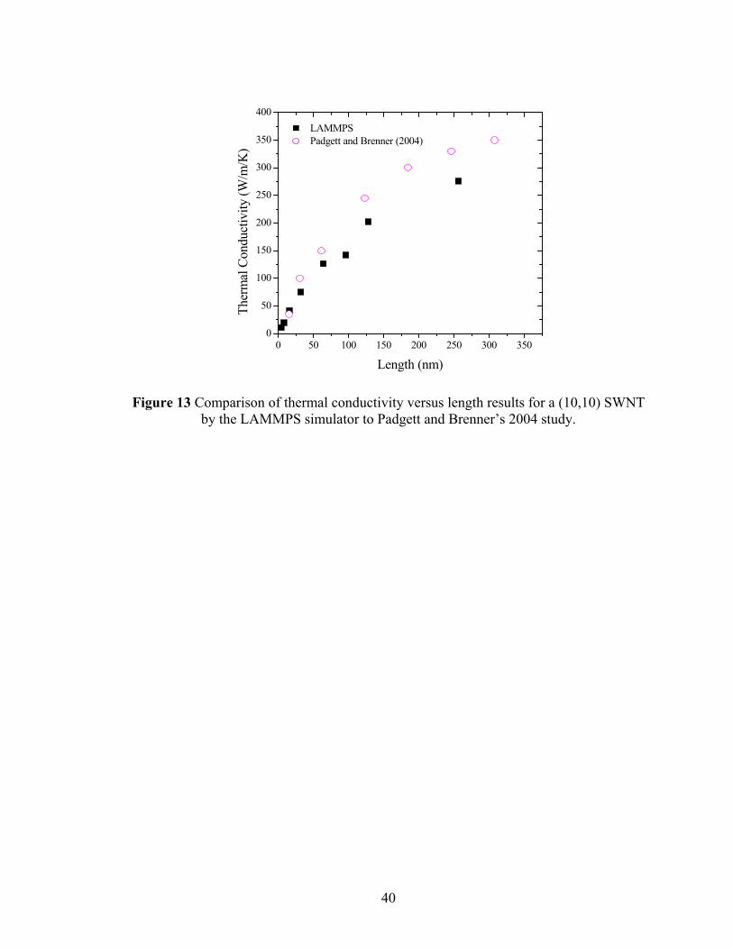
Validation

The simulation setup for the Muller-Plathe NEMD method is compared to Padgett

and Brenner [35] to validate the results of LAMMPS. In their study of the influence of

38

chemisorption, Padgett and Brenner used the Muller-Plathe method to the find the

thermal conductivity of a (10,10) SWNT as a function of length. Using LAMMPS the

simulation was run with their parameters. The chosen interatomic potential was Tersoff

and a time step of 0.25 fs was used. The system was equilibrated at 300 K for 2.5 ps.

The Muller-Plathe method was run for at least 100 ps while swapping the kinetic energy

of 20 atoms every 15 fs. Data is collected and averaged over every 2.5 ps.; the area used

for the SWNT’s cross-section was a 3.4 Å thick ring. The comparison of LAMMPS and

Padgett and Brenner is shown in Figure 13. The results from LAMMPS show the same

trends as Padgett and Brenner’s results—which appear to be approaching a thermal

conductivity limit as the length increases. The divergence of the LAMMPS results from

Padgett and Brenner can be attributed to the SWNT needing a longer time to equilibrate

where the LAMMPS results are equilibrated for 200 ps, which is an order of magnitude

larger than Padgett and Brenner. The LAMMPS results are comparable to Padgett and

Brenner’s data, thus it is valid as a simulator for CNTs.

39

0 50 100 150 200 250 300 3500

50

100

150

200

250

300

350

400

Ther

mal

Con

duct

ivity

(W/m

/K)

Length (nm)

LAMMPS Padgett and Brenner (2004)

Figure 13 Comparison of thermal conductivity versus length results for a (10,10) SWNT

by the LAMMPS simulator to Padgett and Brenner’s 2004 study.

40

CHAPTER V

RESULTS AND DISCUSSION

Carbon nanotube thermal conductivity

Simulations were performed for SWNTs and DWNTs at various lengths from 25

nm-1μm. At 25 nm thermal conductivity for all CNTs studied is ~150 W/m/K; at 1 μm

thermal conductivity ranges from ~1000 W/m/K for the DWNT to >1200 W/m/K for the

(10,10) SWNT (Figure 14). The results presented in Figure 14 show agreement with the

(10,10) SWNT results of Padgett and Brenner [35] (Figure 13). Both results are less than

the values of other computational studies for similar lengths due to the use of the Tersoff

potential [12], [26], [28]. The Tersoff potential overestimates anharmonicities in the

potential and leads to an underestimation of thermal conductivity by ~1000 W/m/K when

compared to experimental measurements [16], [18], [19], [65], [66]. Also the assumption

of the cross-sectional area yields differences in the estimation of thermal conductivity as

mentioned previously. Nevertheless a trend similar to studies of MWNTs and SWNTs

with small diameters is shown [16], [18], [19], since comparable thermal conductivities

are calculated for SWNTs and DWNTs. Unlike previous studies, thermal conductivities

calculated for this study do not converge to a single value, but rather show a general

increasing trend. The increase implies that longer lengths introduce phonon modes of

longer wavelengths that have a significant contribution to thermal conductivity.

Plotting the thermal conductivity versus length on a log-log scale is shown in

Figure 15. Similar to other studies, thermal conductivity in SWNTs is shown to diverge

with increasing length [28], [30]. In 1D model calculations thermal conductivity, λ =

41

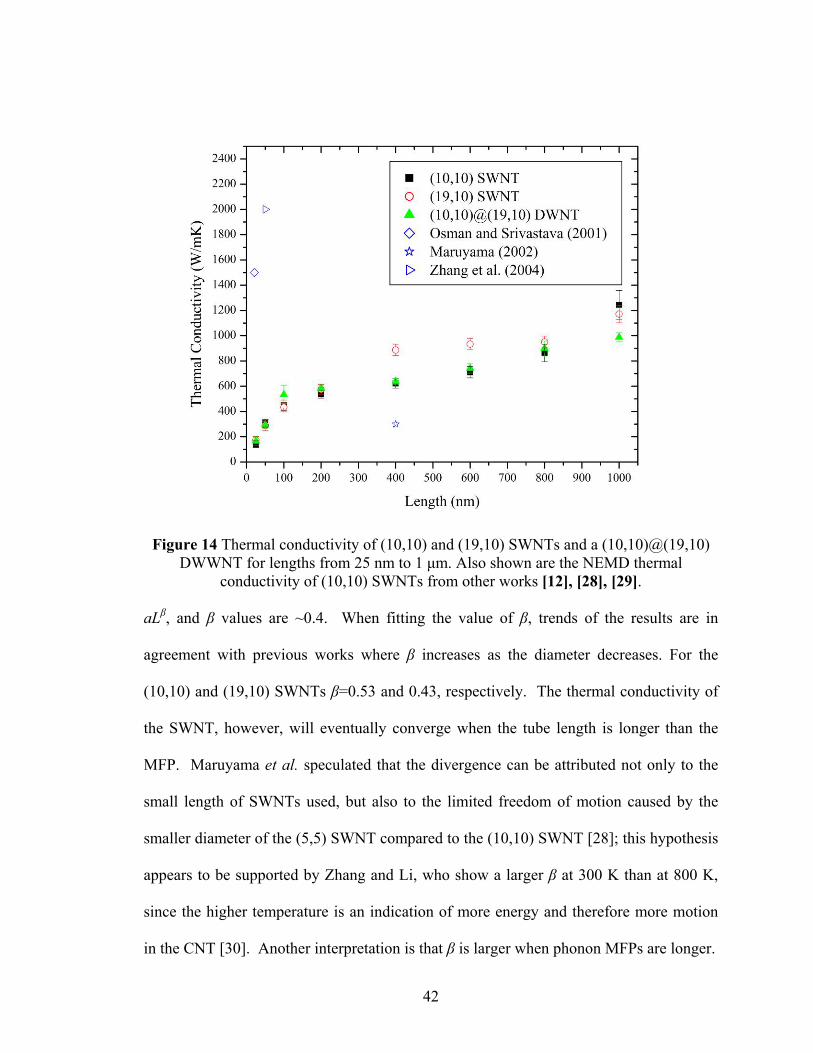
Figure 14 Thermal conductivity of (10,10) and (19,10) SWNTs and a (10,10)@(19,10)

DWWNT for lengths from 25 nm to 1 μm. Also shown are the NEMD thermal conductivity of (10,10) SWNTs from other works [12], [28], [29].

aLβ, and β values are ~0.4. When fitting the value of β, trends of the results are in

agreement with previous works where β increases as the diameter decreases. For the

(10,10) and (19,10) SWNTs β=0.53 and 0.43, respectively. The thermal conductivity of

the SWNT, however, will eventually converge when the tube length is longer than the

MFP. Maruyama et al. speculated that the divergence can be attributed not only to the

small length of SWNTs used, but also to the limited freedom of motion caused by the

smaller diameter of the (5,5) SWNT compared to the (10,10) SWNT [28]; this hypothesis

appears to be supported by Zhang and Li, who show a larger β at 300 K than at 800 K,

since the higher temperature is an indication of more energy and therefore more motion

in the CNT [30]. Another interpretation is that β is larger when phonon MFPs are longer.

42

(a)

(b)

Figure 15 Thermal conductivity versus length plotted on a log-log scale for a (a) (10,10) SWNT and (b) (19,10) SWNT. The line is thermal conductivity λ ~ Lβ.

43

When SWNTs of different chiralities are compared, the average phonon MFP can be

speculated to be longer in the smaller diameter SWNT, since the radial breathing modes

will be smaller and result in fewer phonon-phonon interactions with longer wavelength

phonon modes.

Subsequently, simulations were performed to limit the freedom of motion in the

more to scattering than to thermal transport. Removing or restricting these phonon

CNTs. Double-walled CNTs are modeled that have only one wall heated or only one

wall moving, which is a unique method for isolating a particular vibrational motion and

identifying the contribution of that motion to the thermal conductivity of a CNT. Figure

16 shows the variation of thermal conductivity in DWNTs when the heating scheme is

manipulated. When a single wall is heated and both walls are allowed to move, thermal

conductivity does not deviate largely from the thermal conductivity of the DWNT in the

original setup. The suggestion is van der Waals forces are strong enough to cause the

unheated wall to move in sync with the heated wall; however, the forces are too weak to

cause significant scattering between the walls. Consequently, when one of the walls is

held stationary, the motion of the other wall is significantly restricted because of the van

der Waals forces. The thermal conductivity increases by ~50% in these alternative cases

where one wall is stationary. This result agrees with the trend observed with carbon

peapods [67], which showed thermal conductivities that were twice as large as a pristine

SWNT. Carbon peapods are SWNTs that have fullerenes on the inside. Two

mechanisms of energy transfer were attributed with the increased thermal conductivity: a

low-frequency radial vibration coupling between the CNT and the fullerenes and

collisions between fullerenes along the axis. Some phonon mode interactions contribute

44

Figure 16 Thermal conductivity of DWNT using various heating schemes.

Both walls are moving for the data represented by upside down triangles, but only the exterior wall is heated for the unfilled triangles and only the interior wall for the filled

triangles. In contrast, the diamonds have only one wall moving: only the exterior wall for

in t

to contri is held

yields a low estimation of a modes’ contribution. Computing the mean square vibrational

the unfilled diamonds and the interior wall only for the filled diamonds.

teractions yield a higher thermal conductivity even though fewer phonon modes are lef

bute to thermal conductivity. When either the interior or exterior wall

stationary, the DWNT behaves as a SWNT with restricted motion. A stationary interior

wall restricts flexural modes. Not only flexural modes, but also radial breathing modes

are restricted when the exterior wall is stationary. Longitudinal modes are restricted by

not allowing the LAMMPS’ NVE integrator to update coordinates along the z-axis. This

method is not an entirely perfect way of restricting modes, since the radial breathing and

torsional modes also incorporate longitudinal motion, as well; however, the method

45

amplitudes of atomic motions verifies that vibrational motion is restricted. The Cartesian

coordinates of 25 nm CNTs are converted into cylindrical coordinates for the calculation.

The mean square vibrational amplitude is defined

[ ]∑=

−=N

irru

1

222

21 (5.1)

where α denotes radial (ρ), azimuthal (θ), axial

ii ααα

(z) directons and the brackets <…>

indicate a time average. Table 6 lists the amplitudes for CNTs with different vibrational

mode restrictions. When none of the vibrational modes are restricted the mean-square

vibrational amplitudes in the azimuthal direction is comparable for the SWNT and

DWNT, as well as for the individual walls of the DWNT. This result is expected since the

thermal conductivities are shown to be comparable. The radial and axial directions of the

SWNT and DWNT show differences, which can be attributed to the DWNT having more

vibrations caused by the interaction betweens the walls. The individual walls of the

DWNT, however, show comparable amplitudes. This result is also an indication that the

walls of the DWNT move in sync. In contrast, when all modes except the torsional mode

are restricted the mean-square vibrational amplitudes in the radial and axial directions

decrease by nearly and order of magnitude; meanwhile, the mean-square vibrational

amplitude in the azimuthal direction remains the dominant vibrational direction. Also,

when the flexural mode is present the mean-square vibrational amplitudes are larger in

every direction compared to when the flexural mode is restricted. The flexural mode,

therefore, carries a lot of energy. If the net change in the mean-square vibrational

amplitudes is considered, then the presence of the flexural mode accounts for >80% of

the amplitude increase.

46

Table 6. Mean-square Vibrational amplitudes for 25 nm CNTs with Various

Torsional (T), and/or FCombinations of Vibrational Modes [Longitudinal (L), Radial breathing (B),

lexural (F)] Vibrational Modes (A2) (rad2) <uz

2> (A2)Present

r θ

(10,10)SWNT L-B-T-F 0.060109 0.15209DWNT

0.0014643L-B-T-F 0.85755 0.093327 0.026269

Interior DWNT wall wall

all motion only 0.0011489 ong. 0.084366 0.0017899

ly 0.0010928 ong. ng.

L-B-T-F 1.0662 0.097365 0.0286 Exterior DWNT L-B-T-F 0.94116 0.10889 0.031191Exterior w L-B-T 0.0022555 1.8541e-4(10,10) SWNT w/no l B-T-F 0.14035 Interior wall motion on L-T 0.044124 2.6239e-4Exterior motion only w/no l B-T 0.0013686 0.0030953 2.3844e-4Interior motion only w/no lo T 0.0012941 0.0431 2.1897e-4 The variation of CNT thermal conductivity fro

gure 17. A own, therm vit NT

m different combinations of

phonon modes is presented in Fi s sh al conducti y in SW s is

largely affected by the longitudinal and flexural modes. Thermal conductivity is less than

the unrestricted DWNT when either the torsional mode or the torsional-radial breathing

mode combination is considered. The torsional mode has a smaller thermal conductivity,

because it is the only mode contributing. This result can be expected since in the

Holland[68] and Callaway[69] models of lattice thermal conductivity the thermal

conductivity is a sum of the thermal conductivity contributed by each phonon mode. In

which case, the radial breathing mode is considered to not have an appreciable influence

on thermal conductivity, since its inclusion with the torsional mode results in a thermal

conductivity that is comparable to the torsional mode alone. This result cannot be wholly

contributed to the lack of the longitudinal motion within the breathing and torsional

modes, because thermal conductivity for the longitudinal and torsional mode combination

is comparable to the thermal conductivity of the longitudinal, torsional, and breathing

mode combination. When the flexural mode is added to the torsional and radial breathing

47

Figure 17 Thermal conductivity is shown for the CNT when combinations of modes are

restricted [70]. modes, thermal conductivity increases are directly proportional to length; at 800 nm

thermal conductivity exceeds the unrestricted DWNT. The flexural mode can contribute

more states to the thermal conductivity as the length of the CNT increases. Likewise, as

the length increases the longitudinal mode in combination with torsional and breathing

modes has a thermal conductivity that is greater than the DWNT, because the increased

length adds additional longitudinal mode states that can contribute to thermal

conductivity. However, the combination of the longitudinal and flexural modes in CNTs

result in a thermal conductivity that is lower than either would have with the absence of

the other; an indication that the phonon-phonon interaction of the longitudinal and

48

flexural modes produces scattering resulting in the thermal conductivity seen for the

DWNT.

Thermal conductivity of functionalized carbon nanotubes

the thermal

thermal conductivity when the functionalization atoms are held fixed on the SWNT

The influence of united atom models of phenyl groups on

conductivity of 200 nm SWNTs and DWNTs is studied. Figure 18 shows the results of

thermal conductivity for different densities of functionalization. Thermal conductivity

for a (10,10) SWNT experiences a significant drop with only 0.25% of its atoms

functionalized. The lowest thermal conductivity is shown for 1% functionalization. The

introduction of united atoms creates a phonon scattering site, which effectively reduces

the phonon MFP in the SWNT, thus decreasing thermal conductivity. The results are

similar to those found by Padgett and Brenner for (10,10) SWNT [35]. In contrast, the

(10,10)@(19,10) DWNT’s thermal conductivity increases with a small amount of

functionalization and only begins to decrease between 5% and 10% functionalization

densities, but only slightly. The DWNT has an additional wall that can contribute to

thermal transport, so thermal conductivity is not expected to experience a decrease like

that of the SWNT. The increase of thermal conductivity, however, for the SWNT and

DWNT is unexpected. The increase for the SWNT can be attributed to the increased

functionalization causing the SWNT to approach the behavior of a DWNT. The

functionalizing atoms in the case of the DWNT initially increase thermal conductivity,

because the additional atoms restrict the flexural motion of the DWNT, which increases

thermal conductivity when the longitudinal mode is unrestricted as mentioned in the

previous section. The influence of restricted flexural motion can be corroborated by the

49

Figure 18 Thermal conductivity of a (10,10) SWNT and (10,10)@(19,10) DWNT at different functionalization densities of a phenyl united atom

(F n

manner similar to the DWNT with mobile atoms, but quickly begins to decrease. Small

igure 19). When the functionalizing atoms are fixed, thermal conductivity increases i

a

percentages of functionalization are beneficial to restricting flexural motion in the

SWNT; however, as the amount of fixed functionalizing atoms increase they produce a

larger scattering influence by inhibiting the phonon MFP. In the case of mobile and fixed

functionalizing atoms at 10%, thermal conductivity for the SWNT is the same, which is

an indication the increased functionalization is influencing the SWNT’s thermal

conductivity to approach that of the DWNT.

50

Figure 19 Thermal conductivity of (10,10) SWNT when the functionalizing atoms are

mobile and fixed. The influence on thermal conductivity of a 200 nm (10,10) SWNT is shown as the

v

toms has an equilibrium position that can be closer to the CNT, the influence of σ is

stronger when the distance is smaller. As σ increases and, consequently, the equilibrium

position is further away the interaction with the CNT begins to weaken. Thermal

conductivity is shown in Figure 20 for a 1% functionalized (10,10) SWNT. The error is

large in this measurement since the functionalizing atoms are mobile and can move

between the regions used to produce the temperature gradient during the simulation. The

general trend that can be deduced from the thermal conductivity is a decrease as σ

increases. When the value of σ is small and it has a stronger interaction with the SWNT,

alue of the Lennard-Jones parameter σ is varied. When σ is small the functionalizing

a

51

the flexural modes are restricted allowing a larger thermal conductivity; however, as σ

increases its influence is weaker and it become a scattering site disrupting the phonon

MFP in the SWNT.

Table 7. Mean-square Vibrational amplitudes for 200 nm functionalized SWNTs

Density of Functionalization <ur2> (A2) <uθ2> (rad2) <uz

2> (A2) with Various Functalization Densities

0% 24.037 0.16173 4.7263 0.25% 10.006 0.53713 0.71162

10% 14.732

1% 33.893 0.21437 1.0755 5% 2 .75 66 0.65069

0.017392 11.129 1.8167

Figure 20 Thermal conductivity of (10,10) SWNT as the Lennard-Jones parameter σ is

varied

52

Results from varying ε are not shown, because no substantial change in thermal

conductivity was observed. This result is not surprising when the Lennard-Jones

potential is considered. When the first derivative of the Lennard-Jones potential is

considered with respect to ε, the following equation results

⎥⎦

⎤⎢⎣

⎡−=

∂∂

6

6

12

12

4rr

U σσε

(5.2)

The slope of the potential as ε is varied is a constant, so no large changes in thermal

conductivity should result by changing ε. When the first derivative of the Lennard-Jones

potential is considered with respect to σ, the following equation results

⎥⎦

⎤⎢⎣

⎡+−−=

∂∂

7

6

6

5

13

12

12

11

6612124rrrr

U σσσσεσ

(5.3)

The slope indicates that shape of the potential changes when varying σ. The value of σ

w

the united atoms.

σ r θ z

ill, therefore, model the strengthening and weakening of the bond between the CNT and

Table 8. Mean-square Vibrational amplitudes for 200 nm 1% functionalized SWNT with Various σ Values

(A2) (Å2) (rad2) (Å2)

2.0 13.883 0.25255 4.4366 2.5 8.1334 0.41734 4.8955 3.0 21.848 0.13979 12.441 3.5 6.1615 0.4.0 5.6616 0.32959 4.5 10.185 0.23802 3.2807

29029 3.4952 6.4162

53

Thermal Conductivity in Graphene

Thermal conductivity of graphene is show in Figure 21 for graphene confined in

e directly compared; however, graphene does serve as a model for the

conductivities show a similar trend Ts studied. The

thermal conductivity values, however, are larger for graphene when compared to CNTs

of a similar length in Figure 14. e C ddi onon modes, the

phonon-phonon interactions cause ad scatt pre raphene [66]. The

results of the N D simulation are ble to those reported by others [54]. Of the

ngle modes’ thermal conductivity, the flexural mode shows the lowest overall;

however, the result woul al mode does incorporate

each vibrational direction (longitudinal, transverse, and flexural). Graphene can be

considered an unrolled SWNT. Since graphene is 2-D versus the 3-D CNT, the two

materials cannot b

behavior of a SWNT with no torsional or radial breathing modes. The thermal

in the length-dependence as the CN

Since th NT has a tional ph

ditional ering not sent in g

EM compara

si

d be a low estimation, since the flexur

longitudinal motion, as well. The longitudinal and transverse modes have thermal

conductivities lower than unrestricted graphene, which is due to the lack of modes to

contribute to energy transport as mentioned earlier. With combinations containing two

modes, the flexural mode appears to introduce phonon-phonon interactions that do not

enhance thermal conductivity. Thermal conductivity increases from that observed with

only the flexural mode, since the other two modes add phonon modes; however, the

thermal conductivity is less than the result of the longitudinal or transverse mode alone.

The out of plane motion of the flexural mode leads to a shorter MFP in the graphene,

because the forces between the surrounding atoms is altered as the atoms are cause to

move closer together due to the interatomic potential. Furthermore, the influence of the

54

flexural mode can be noticed when comparing thermal conductivities of unrestricted

graphene to the combination of longitudinal and transverse modes: thermal conductivity

is larger for the two mode combination, since there is no disruptive out of plane motion.

The behavior of the graphene is beneficial in understanding thermal transport in

the CNT. Since torsional and radial breathing modes are not present in graphene, it can

be speculated that modes that incorporate longer wavelength phonons with increasing

length dominate thermal conductivity in both graphene and CNTs. Because the CNT’s

interatomic potential limits the vibrational motion of the atoms for the torsional and

radial breathing modes, the larger influence on thermal conductivity will come from

longitudinal and flexural modes, which will have a larger range of vibrational motion and

also longer wavelengths of phonons.

55

Figure 21 Thermal conductivity of graphene that is confined in various directions.

56

CHAPTER VI

CONCLUSIONS

Non-equilibrium MD simulations are used to investigate the influence of

individual phonon on vibrational modes on the thermal conductivity in SWNTs and

DWNTs. Additionally, functionalized CNTs are modeled using united atom models of

phenyl to investigate the influence of functionalization on the vibrational modes and

graphene confined in various directions is studied. Unlike previous studies that show

thermal conductivity converging at short sample lengths, thermal conductivity of (10,10)

and (19,10) SWNTs and (10,10)@(19,10) DWNTs is shown to continue increasing

beyond 800 nm. Using the DWNT to confine the motion of the SWNTs, the vibrational

modes are isolated and show thermal conductivity to be largely influence by the

contribution of longitudinal and flexural modes. The phonon-phonon interaction of the

flexural mode and longitudinal mode, however, causes degradation to thermal

conductivity of CNT. The influence of suppressing the flexural mode is also seen in the

thermal conductivity of functionalized (10,10) SWNTs. Though the SWNT experiences

a decrease in thermal conductivity with only a small percentage of united atom phenyl

groups functionalizing it, the DWNT does not show any decrease in thermal conductivity.

Unexpectedly, both functionalized CNTs experience an increase in thermal conductivity

attributed to the suppression of the flexural mode. While investigating the influence on

bond strength on thermal conductivity using the Lennard-Jones parameters σ and ε,

thermal conductivity in SWNTs was shown to have a slight response to altering σ, which

57

corresponds to weakening and strengthening the bond. Thermal conductivity was higher

with smaller σ values—an indication that the stronger bond was also a method of

suppressing flexural motion in the SWNT. Furthermore, graphene is shown to have a

thermal conductivity trends that are similar to CNTs, but higher in value since there is

less phonon-phonon interaction. When confining the vibrational mode, graphene also

shows the flexural mode to contribute to the degradation of conductivity.

The results show promise in using CNTs in thermal management applications.

Though the SWNT cannot be functionalized for use in thermal enhancement applications,

DWNTs and MWNTs offer an alternative, since their interior walls offer additional

pathway to transport heat even though the exterior wall may be treated. For this reason,

open-ended tubes will offer better access to the CNT’s interior walls than CNTs that have

capped ends. When processing CNTs longer samples will largely yield better thermal

conductivity as long as the length of the system is not in the diffusive regime; therefore,

processing techniques that do not break the CNT will be more desirable. Graphene

shows similar disadvantages as the SWNT, since scattering can be cause by treatment;

however, films of a few layers of graphene may offer advantages similar to MWNTs.

Major contributions to the field of study include

• A length-dependent study of thermal conductivity in DWNTs using MD

simulations,

• Confinement of vibrational motion in MD simulations,

• Altering the Lennard-Jones potential parameters σ and ε to study their influence

on thermal conductivity

58

Future Work

There are some extensions to this work that may offer further insight to the

behavior of CNTs in thermal applications. In the current work, united atom models were

utilized to study the influence of bond strength on thermal conductivity. By using an

explicit atom model, a more accurate study of the influence of bond strength and atom

interaction can be performed. Furthermore, the use of a interatomic potential that

describes covalent bonds will yield a better picture of the scattering cause by chemical

treatments to the CNT. Since the broader goal is to understand better techniques for

using CNTs as fillers, future studies should extend these efforts to nanocomposite

samples. Models of hydrocarbons are readily described by the covalently bonding

interatomic potentials in this study. Time steps, minimization, and equilibration will

require much scrutiny when moving to the nanocomposite sample.

In addition to modifing the model of the CNT, studying other materials is a route

of interest as well. Graphene was only considered in small instances here, but the

influence of functionalization and defects on its thermal conductivity open a new

direction for study. Also, boron nitride nanotubes have received consideration in thermal

studies. Understanding the phonon behavior in theses materials offer a method of

comparison to CNTs.

59

APPENDIX A

SIMULATION SCRIPTS

TubeGen Script

The following is a script that generates 150 unit cells of a (10,10) SWNT and

outputs the results to a file named data.cnt.

set relax_tube yes set format xyz set units angstrom set element1 C set element2 C set chirality 10,10 set bond 1.4210 set shape hexagonal set gutter 5.0000, 5.0000, 0.0000 set cell_count 1,1,150 generate save data.cnt exit

LAMMPS script

The following LAMMPS scripts produce the thermal conductance for a 100 nm

(5,5) SWNT under various conditions. LAMMPS is frequently updated; therefore, the

latest version may not support the commands present in this script.

Script for Single-wall Carbon Nanotube Thermal Conductance

clear log log.swnt5,5-100nm ###Simulation of thermal conductivity for a single-walled carbon nanotube### ###Initialization###

60

units metal dimension 3 atom_style atomic boundary p p p processors 1 1 20 #Atom definition read_data cnt/swnt8960-5,5-100nm+b.minimized region wall1 block INF INF INF INF INF 10 units box region cold block INF INF INF INF 10 50 units box region tube block INF INF INF INF 50 1050 units box region hot block INF INF INF INF 1050 1091 units box region wall2 block INF INF INF INF 1091 INF units box #Settings and Simulation pair_style tersoff pair_coeff * * ../../LAMMPS/lammps-20Aug11/potentials/SiC.tersoff C mass * 12 group wall1 region wall1 group wall2 region wall2 group cold region cold group hot region hot group tube region tube group nowalls union cold tube hot ###EQUILIBRATION### neighbor 2.0 bin neigh_modify every 3 delay 3 velocity nowalls create 300.0 49284121 fix 1 nowalls nve #dump 1 all custom 10000 dump.nemd.swnt-1000A_b tag type x y z #dump 2 all xyz 500 dump.nemd.swnt-1000A_b.movie variable g_ke equal ke(tube) variable g_temp equal v_g_ke/1.5/8.617343e-5/8130 thermo 2000 thermo_style custom step temp ke etotal v_g_temp timestep 0.001 run 200000 ###NEMD### #--CONSTANT FLUX--# fix 3 cold heat 1 -5 fix 4 hot heat 1 5 compute coldBath cold temp compute hotBath hot temp thermo 2000 thermo_style custom step temp ke etotal v_g_temp c_coldBath c_hotBath

61

run 500000 log logs/log.data_collect-swnt5,5-100nm_b ###DATA COLLECTION### compute KE tube ke/atom variable temp atom c_KE[]/1.5/8.617343e-5 fix 5 tube ave/spatial 200 1 200 z middle 55.1 v_temp file & temp_profile/tmp.profile-swnt5,5-100nm_b units box thermo 2000 thermo_style custom step temp ke etotal v_g_temp c_coldBath c_hotBath run 500000

62

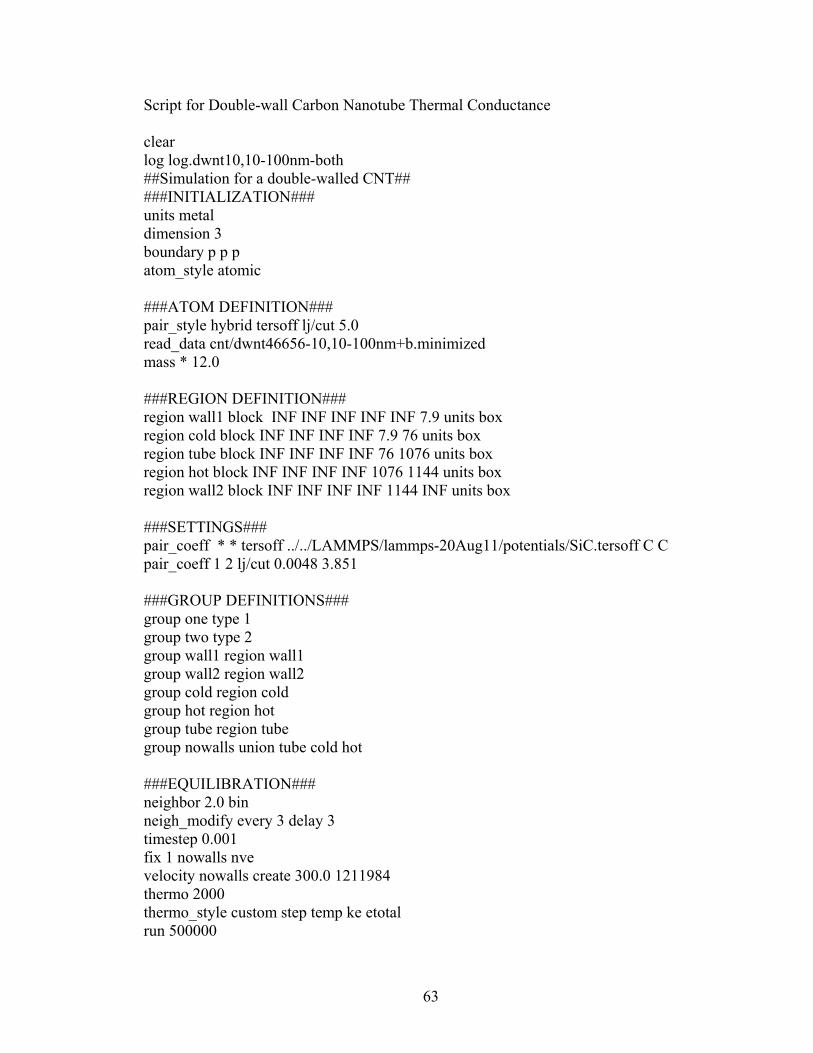
Script for Double-wall Carbon Nanotube Thermal Conductance

clear log log.dwnt10,10-100nm-both ##Simulation for a double-walled CNT## ###INITIALIZATION### units metal dimension 3 boundary p p p atom_style atomic ###ATOM DEFINITION### pair_style hybrid tersoff lj/cut 5.0 read_data cnt/dwnt46656-10,10-100nm+b.minimized mass * 12.0 ###REGION DEFINITION### region wall1 block INF INF INF INF INF 7.9 units box region cold block INF INF INF INF 7.9 76 units box region tube block INF INF INF INF 76 1076 units box region hot block INF INF INF INF 1076 1144 units box region wall2 block INF INF INF INF 1144 INF units box ###SETTINGS### pair_coeff * * tersoff ../../LAMMPS/lammps-20Aug11/potentials/SiC.tersoff C C pair_coeff 1 2 lj/cut 0.0048 3.851 ###GROUP DEFINITIONS### group one type 1 group two type 2 group wall1 region wall1 group wall2 region wall2 group cold region cold group hot region hot group tube region tube group nowalls union tube cold hot ###EQUILIBRATION### neighbor 2.0 bin neigh_modify every 3 delay 3 timestep 0.001 fix 1 nowalls nve velocity nowalls create 300.0 1211984 thermo 2000 thermo_style custom step temp ke etotal run 500000

63

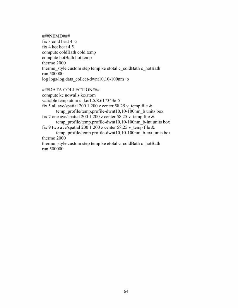
###NEMD### fix 3 cold heat 4 -5 fix 4 hot heat 4 5 compute coldBath cold temp compute hotBath hot temp thermo 2000 thermo_style custom step temp ke etotal c_coldBath c_hotBath run 500000 log logs/log.data_collect-dwnt10,10-100nm+b ###DATA COLLECTION### compute ke nowalls ke/atom variable temp atom c_ke/1.5/8.617343e-5 fix 5 all ave/spatial 200 1 200 z center 58.25 v_temp file & temp_profile/temp.profile-dwnt10,10-100nm_b units box fix 7 one ave/spatial 200 1 200 z center 58.25 v_temp file & temp_profile/temp.profile-dwnt10,10-100nm_b-int units box fix 9 two ave/spatial 200 1 200 z center 58.25 v_temp file & temp_profile/temp.profile-dwnt10,10-100nm_b-ext units box thermo 2000 thermo_style custom step temp ke etotal c_coldBath c_hotBath run 500000

64

Script for Double-wall Carbon Nanotube with Interior Wall Heated

clear log log.dwnt10,10-100nm-int ##Simulation for a double-walled CNT## ###INITIALIZATION### units metal dimension 3 boundary p p p atom_style atomic ###ATOM DEFINITION### pair_style hybrid tersoff lj/cut 5.0 read_data cnt/dwnt46656-10,10-100nm+b.minimized mass * 12.0 ###REGION DEFINITION### region wall1 block INF INF INF INF INF 7.9 units box region cold block INF INF INF INF 7.9 76 units box region tube block INF INF INF INF 76 1076 units box region hot block INF INF INF INF 1076 1144 units box region wall2 block INF INF INF INF 1144 INF units box region cold_inner cylinder z 0 0 7 7.9 76 units box region cold_entire cylinder z 0 0 12 7.9 76 units box region hot_inner cylinder z 0 0 7 1076 1144 units box region hot_entire cylinder z 0 0 12 1076 1144 units box ###SETTINGS### pair_coeff * * tersoff ../../LAMMPS/lammps20Aug11/potentials/SiC.tersoff C C pair_coeff 1 2 lj/cut 0.0048 3.851 ###GROUP DEFINITIONS### group one type 1 group two type 2 group wall1 region wall1 group wall2 region wall2 group cold region cold group hot region hot group tube region tube group cold_entire region cold_entire group hot_entire region hot_entire group cold_inner region cold_inner group hot_inner region hot_inner group nowalls union tube cold hot ###EQUILIBRATION###

65

neighbor 2.0 bin neigh_modify every 3 delay 3 timestep 0.001 fix 1 nowalls nve velocity nowalls create 300.0 1211984 thermo 2000 thermo_style custom step temp ke etotal run 500000 ###NEMD### fix 3 cold_inner heat 4 -5 fix 4 hot_inner heat 4 5 compute coldBath cold_inner temp compute hotBath hot_inner temp thermo 2000 thermo_style custom step temp ke etotal c_coldBath c_hotBath run 500000 log logs/log.data_collect_int-dwnt10,10-100nm_b ###DATA COLLECTION### compute ke nowalls ke/atom variable temp atom c_ke/1.5/8.617343e-5 fix 5 all ave/spatial 200 1 200 z center 58.25 v_temp file & temp_profile/temp.profile_intt-dwnt10,10-100nm_b units box fix 7 one ave/spatial 200 1 200 z center 58.25 v_temp file & temp_profile/temp.profile_int-dwnt10,10-100nm_b-int units box fix 9 two ave/spatial 200 1 200 z center 58.25 v_temp file & temp_profile/temp.profile_int-dwnt10,10-100nm_b-ext units box thermo 2000 thermo_style custom step temp ke etotal c_coldBath c_hotBath run 500000

66

Script for Double-wall Carbon Nanotube with Interior Wall Heated

clear log log.dwnt10,10-100nm-ext ##Simulation for a double-walled CNT## ###INITIALIZATION### units metal dimension 3 boundary p p p atom_style atomic ###ATOM DEFINITION### pair_style hybrid tersoff lj/cut 8.0 read_data cnt/dwnt46656-10,10-100nm+b.minimized mass * 12.0 ###REGION DEFINITION### region wall1 block INF INF INF INF INF 7.9 units box region cold block INF INF INF INF 7.9 76 units box region tube block INF INF INF INF 76 1076 units box region hot block INF INF INF INF 1076 1144 units box region wall2 block INF INF INF INF 1144 INF units box region cold_inner cylinder z 0 0 7 7.9 76 units box region cold_entire cylinder z 0 0 12 7.9 76 units box region hot_inner cylinder z 0 0 7 1076 1144 units box region hot_entire cylinder z 0 0 12 1076 1144 units box ###SETTINGS### pair_coeff * * tersoff ../../LAMMPS/lammps-20Aug11/potentials/SiC.tersoff C C pair_coeff 1 2 lj/cut 0.0048 3.851 ###GROUP DEFINITIONS### group one type 1 group two type 2 group wall1 region wall1 group wall2 region wall2 group cold region cold group hot region hot group tube region tube group cold_entire region cold_entire group hot_entire region hot_entire group cold_inner region cold_inner group hot_inner region hot_inner group nowalls union tube cold hot group chiller subtract cold_entire cold_inner group heater subtract hot_entire hot_inner

67

###EQUILIBRATION### neighbor 2.0 bin neigh_modify every 3 delay 3 timestep 0.001 fix 1 nowalls nve velocity nowalls create 300.0 1211984 thermo 2000 thermo_style custom step temp ke etotal run 500000 ###NEMD### fix 3 chiller heat 4 -5 fix 4 heater heat 4 5 compute coldBath chiller temp compute hotBath heater temp thermo 2000 thermo_style custom step temp ke etotal c_coldBath c_hotBath run 500000 log logs/log.data_collect_ext-dwnt10,10-100nm_b ###DATA COLLECTION### compute ke nowalls ke/atom variable temp atom c_ke/1.5/8.617343e-5 fix 5 all ave/spatial 200 1 200 z center 58.25 v_temp file & temp_profile/temp.profile_ext-dwnt10,10-100nm_b units box fix 7 one ave/spatial 200 1 200 z center 58.25 v_temp file & temp_profile/temp.profile_ext-dwnt10,10-100nm_b-int units box fix 9 two ave/spatial 200 1 200 z center 58.25 v_temp file & temp_profile/temp.profile_ext-dwnt10,10-100nm_b-ext units box thermo 2000 thermo_style custom step temp ke etotal c_coldBath c_hotBath run 500000

68

Script for Double-wall Carbon Nanotube with Exterior Wall Moving

clear log log.dwnt10,10-100nm-ext_only ##Simulation for a double-walled CNT## ###INITIALIZATION### units metal dimension 3 boundary p p p atom_style atomic ###ATOM DEFINITION### pair_style hybrid tersoff lj/cut 8.0 read_data cnt/dwnt46656-10,10-100nm+b.minimized mass * 12.0 ###REGION DEFINITION### region wall1 block INF INF INF INF INF 7.9 units box region cold block INF INF INF INF 7.9 76 units box region tube block INF INF INF INF 76 1076 units box region hot block INF INF INF INF 1076 1144 units box region wall2 block INF INF INF INF 1144 INF units box region cold_inner cylinder z 0 0 7 7.9 76 units box region cold_entire cylinder z 0 0 12 7.9 76 units box region hot_inner cylinder z 0 0 7 1076 1144 units box region hot_entire cylinder z 0 0 12 1076 1144 units box ###SETTINGS### pair_coeff * * tersoff ../../LAMMPS/lammps-20Aug11/potentials/SiC.tersoff C C pair_coeff 1 2 lj/cut 0.0048 3.851 ###GROUP DEFINITIONS### group one type 1 group two type 2 group wall1 region wall1 group wall2 region wall2 group cold region cold group hot region hot group tube region tube group cold_entire region cold_entire group hot_entire region hot_entire group cold_inner region cold_inner group hot_inner region hot_inner group nowalls union tube cold hot group chiller subtract cold_entire cold_inner group heater subtract hot_entire hot_inner

69

group sample subtract two wall1 wall2 ###EQUILIBRATION### neighbor 2.0 bin neigh_modify every 3 delay 3 timestep 0.001 fix 1 sample nve velocity nowalls create 300.0 1211984 thermo 2000 thermo_style custom step temp ke etotal run 200000 ###NEMD### fix 3 chiller heat 4 -5 fix 4 heater heat 4 5 compute coldBath chiller temp compute hotBath heater temp thermo 2000 thermo_style custom step temp ke etotal c_coldBath c_hotBath run 500000 log logs/log.data_collect_ext_only-dwnt10,10-100nm_b ###DATA COLLECTION### compute ke nowalls ke/atom variable temp atom c_ke/1.5/8.617343e-5 fix 5 all ave/spatial 200 1 200 z center 58.25 v_temp file & temp_profile/temp.profile_ext_only-dwnt10,10-100nm_b units box fix 7 one ave/spatial 200 1 200 z center 58.25 v_temp file & temp_profile/temp.profile_ext_only-dwnt10,10-100nm_b-int units box fix 9 two ave/spatial 200 1 200 z center 58.25 v_temp file & temp_profile/temp.profile_ext_only-dwnt10,10-100nm_b-ext units box thermo 2000 thermo_style custom step temp ke etotal c_coldBath c_hotBath run 500000

70

Script for Double-wall Carbon Nanotube with Interior Wall Moving

clear log log.dwnt10,10-100nm-int_only ##Simulation for a double-walled CNT## ###INITIALIZATION### units metal dimension 3 boundary p p p atom_style atomic ###ATOM DEFINITION### pair_style hybrid tersoff lj/cut 5.0 read_data cnt/dwnt46656-10,10-100nm+b.minimized mass * 12.0 ###REGION DEFINITION### region wall1 block INF INF INF INF INF 7.9 units box region cold block INF INF INF INF 7.9 76 units box region tube block INF INF INF INF 76 1076 units box region hot block INF INF INF INF 1076 1144 units box region wall2 block INF INF INF INF 1144 INF units box region cold_inner cylinder z 0 0 7 7.9 76 units box region cold_entire cylinder z 0 0 12 7.9 76 units box region hot_inner cylinder z 0 0 7 1076 1144 units box region hot_entire cylinder z 0 0 12 1076 1144 units box ###SETTINGS### pair_coeff * * tersoff ../../LAMMPS/lammps-20Aug11/potentials/SiC.tersoff C C pair_coeff 1 2 lj/cut 0.0048 3.851 ###GROUP DEFINITIONS### group one type 1 group two type 2 group wall1 region wall1 group wall2 region wall2 group cold region cold group hot region hot group tube region tube group cold_entire region cold_entire group hot_entire region hot_entire group cold_inner region cold_inner group hot_inner region hot_inner group nowalls union tube cold hot group sample subtract one wall1 wall2

71

###EQUILIBRATION### neighbor 2.0 bin neigh_modify every 3 delay 3 timestep 0.001 fix 1 sample nve velocity nowalls create 300.0 1211984 thermo 2000 thermo_style custom step temp ke etotal run 500000 ###NEMD### fix 3 cold_inner heat 4 -5 fix 4 hot_inner heat 4 5 compute coldBath cold_inner temp compute hotBath hot_inner temp thermo 2000 thermo_style custom step temp ke etotal c_coldBath c_hotBath run 500000 log logs/log.data_collect_int_only-dwnt10,10-100nm_b ###DATA COLLECTION### compute ke nowalls ke/atom variable temp atom c_ke/1.5/8.617343e-5 fix 5 all ave/spatial 200 1 200 z center 58.25 v_temp file & temp_profile/temp.profile_int_only-dwnt10,10-100nm_b units box fix 7 one ave/spatial 200 1 200 z center 58.25 v_temp file & temp_profile/temp.profile_int_only-dwnt10,10-100nm_b-int units box fix 9 two ave/spatial 200 1 200 z center 58.25 v_temp file & temp_profile/temp.profile_int_only-dwnt10,10-100nm_b-ext units box thermo 2000 thermo_style custom step temp ke etotal c_coldBath c_hotBath run 500000

72

Script for Functionalized Single-wall Carbon Nanotube

clear log log.fswnt10,10-200nm-1% ##Simulation for a double-walled CNT## ###INITIALIZATION### units metal dimension 3 boundary p p p atom_style atomic ###ATOM DEFINITION### pair_style hybrid tersoff lj/cut 5.0 read_data /workspace/walkere1/func33844-10,10-200nm+b-1%-1.minimized mass 1 12.0 mass 2 77.0 ###SETTINGS### pair_coeff * * tersoff ../../local/lammps-4Dec11/potentials/SiC.tersoff C NULL pair_coeff 1 2 lj/cut 0.0035 3.7755 pair_coeff 2 2 lj/cut 0.0026 3.7 ###GROUP DEFINITIONS### group one type 1 group two type 2 group wall1 id <= 260 group wall2 id <> 33261 33520 group cold id <> 261 520 group hot id <> 33001 33260 group tube id <> 521 33000 group sample union tube cold hot group nowalls union tube cold hot two ###EQUILIBRATION### neighbor 2.0 bin neigh_modify every 3 delay 3 variable m loop 3 label loop1 if "$m > 4" then "jump script/in.fswnt200-1 exitloop1" minimize 0.0 1e-8 100000 1000000 fix 2 all nve velocity all set 0.0 0.0 0.0 units box run 100

73

unfix 2 next m jump script/in.fswnt200-1 loop1 label exitloop1 timestep 0.001 fix 1 nowalls nve velocity nowalls create 300.0 1211984 variable g_ke equal ke(sample) variable g_temp equal v_g_ke/1.5/8.6173743e-5/33000 thermo 2000 thermo_style custom step temp ke etotal v_g_temp run 50000 label test if "(${g_temp} > 297.0) && (${g_temp} < 303.0)" then & "jump script/in.fswnt200-1 break" & else & "velocity sample scale 300.0" "run 10000" "jump script/in.fswnt200-1 test" label break reset_timestep 0 ###DATA COLLECTION### dump 1 tube custom 10 /workspace/walkere1/dump25_1/*.fswnt200-1.dos id type xu yu zu vx vy vz dump_modify 1 sort id dump 2 two custom 10 /workspace/walkere1/dump25_1/fatoms/*.fatoms200-1.dos id type xu yu zu vx vy vz dump_modify 2 sort id run 50000

74

Script for Functionalized Double-wall Carbon Nanotube

clear log log.funcd10,10-200nm-1% ##Simulation for a double-walled CNT## ###INITIALIZATION### units metal dimension 3 boundary p p p atom_style atomic ###ATOM DEFINITION### pair_style hybrid tersoff lj/cut 5.0 read_data cnt/func93782-10,10-200nm+b-1%-2.minimized mass * 12.0 mass 3 77.0 ###REGION DEFINITION### region wall1 block INF INF INF INF INF 16.3 units box region cold block INF INF INF INF 16.3 152 units box region tube block INF INF INF INF 152 2152 units box region hot block INF INF INF INF 2152 2288 units box region wall2 block INF INF INF INF 2288 INF units box ###SETTINGS### pair_coeff * * tersoff ../lammps-7Apr11/potentials/SiC.tersoff C C NULL pair_coeff 1 2 lj/cut 0.0048 3.851 pair_coeff 1 3 lj/cut 0.0010 3.55 pair_coeff 2 3 lj/cut 0.0010 3.55 pair_coeff 3 3 lj/cut 0.0026 3.7 ###GROUP DEFINITIONS### group one type 1 group two type 2 group three type 3 group wall1 region wall1 group wall2 region wall2 group cold region cold group hot region hot group tube region tube group nowalls union tube cold hot ###EQUILIBRATION###

75

neighbor 2.0 bin neigh_modify every 3 delay 3 timestep 0.001 fix 1 nowalls nve velocity nowalls create 300.0 1211984 dump 1 all xyz 5000 /workspace/walkere1/fdwnt10,10-200nm+b-1.xyz thermo 2000 thermo_style custom step temp ke etotal run 100000 ###NEMD### fix 3 cold heat 5 -2 fix 4 hot heat 5 2 compute coldBath cold temp compute hotBath hot temp thermo 2000 thermo_style custom step temp ke etotal c_coldBath c_hotBath run 500000 log logs/log.data_collect-funcd10,10-200nm+b-1% ###DATA COLLECTION### compute ke nowalls ke/atom variable temp atom c_ke/1.5/8.617343e-5 fix 5 all ave/spatial 200 1 200 z center 116.25 v_temp file & temp_profile/temp.profile-fdwnt10,10-200nm_b-1% units box fix 7 one ave/spatial 200 1 200 z center 116.25 v_temp file & temp_profile/temp.profile-fdwnt10,10-200nm_b-1%-int units box fix 9 two ave/spatial 200 1 200 z center 116.25 v_temp file & temp_profile/temp.profile-fdwnt10,10-200nm_b-1%-ext units box fix 11 three ave/spatial 200 1 200 z center 116.25 v_temp file & temp_profile/temp.profile-fdwnt10,10-200nm_b-1%-func units box thermo 2000 thermo_style custom step temp ke etotal c_coldBath c_hotBath run 1000000

76

Script for Graphene Thermal Conductance

clear log log.graphene-10,10-100nm #Simulation of thermal conductivity for a single-walled carbon nanotube #Initialization units metal atom_style atomic boundary p p p #processors 1 1 20 #Atom definition read_data crystal/graphene32520-10,10-200nm #Settings and Simulation pair_style tersoff pair_coeff * * ../../../../../LAMMPS/lammps-20Aug11/potentials/SiC.tersoff C mass 1 12 neighbor 2.0 bin neigh_modify every 3 delay 3 timestep 0.001 thermo 2000 thermo_style custom step temp ke etotal pe variable m loop 3 label loop1 if "$m > 3" then "jump script/in.graphene100 exitloop1" minimize 0.0 1e-8 100000 1000000 fix 2 all nve velocity all set 0.0 0.0 0.0 units box run 100 unfix 2 next m jump script/in.graphene100 loop1 label exitloop1 velocity all create 300.0 1211984 fix 1 all nve #dump 1 all custom 10000 dump.nemd.swnt-100nm tag type x y z #dump 2 all xyz 10000 dump.nemd.swnt-100nm.movie

77

run 200000 reset_timestep 0 fix KEswap all thermal/conductivity 50 z 20 swap 20 compute KE all ke/atom variable temp atom c_KE/1.5/8.617343e-5 fix 3 all ave/spatial 2000 1 2000 z lower 100 & v_temp file temp.profile-graphene10,10-100nm units box thermo 2000 thermo_style custom step temp ke etotal f_KEswap run 1000000

78

Script for Bilayer Graphene Thermal Conductance

clear log log.bilayer-10,10-100nm #Simulation of thermal conductivity for a single-walled carbon nanotube #Initialization units metal atom_style atomic boundary p p p #processors 1 1 20 #Atom definition read_data crystal/bilayer65040-10,10-200nm #Settings and Simulation pair_style hybrid tersoff lj/cut 5.0 pair_coeff * * tersoff ../../../../../LAMMPS/lammps-20Aug11/potentials/SiC.tersoff C C pair_coeff 1 2 lj/cut 0.0048 3.851 mass * 12 group one type 1 group two type 2 neighbor 2.0 bin neigh_modify every 3 delay 3 timestep 0.001 thermo 2000 thermo_style custom step temp ke etotal pe variable m loop 3 label loop1 if "$m > 3" then "jump script/in.bilayer100 exitloop1" minimize 0.0 1e-8 100000 1000000 fix 2 all nve velocity all set 0.0 0.0 0.0 units box run 100 unfix 2 next m jump script/in.bilayer100 loop1 label exitloop1 velocity all create 300.0 1211984

79

80

fix 1 one nve #dump 1 all custom 10000 dump.nemd.swnt-100nm tag type x y z dump 2 all xyz 10000 /scratch/walkere1/bilayer-lower_nve-100nm.xyz run 200000 #reset_timestep 0 fix KEswap one thermal/conductivity 50 z 20 swap 20 compute KE all ke/atom variable temp atom c_KE/1.5/8.617343e-5 fix 3 all ave/spatial 2000 1 2000 z lower 100 & v_temp file temp.profile-bilayer10,10-100nm units box fix 4 one ave/spatial 2000 1 2000 z lower 100 & v_temp file temp.profile-bilayer10,10-100nm-lower units box fix 5 two ave/spatial 2000 1 2000 z lower 100 & v_temp file temp.profile-bilayer10,10-100nm-upper units box thermo 2000 thermo_style custom step temp ke etotal f_KEswap run 1000000

APPENDIX B

RAW THERMAL CONDUCTIVITY DATA

Table 9 Thermal Conductivity of CNTs Length (nm)

(5,5) SWNT (W/m/K)

Error (10,10) SWNT (W/m/K)

Error (19,10) SWNT (W/m/K)

Error (10,10)@(19,10) DWNT (W/m/K)

Error

25 170.99666 29.33374 140.92182 25.59983 173.48272 28.05006 166.25662 31.90126 50 263.3963 41.29698 306.49064 31.53486 290.84733 42.07485 293.75032 29.72806 100 414.76315 49.20131 449.55952 41.31526 433.57847 36.55526 534.54005 71.91429 200 518.40133 72.92037 536.72015 31.66977 574.50649 40.30291 581.87192 26.02082 400 890.863 81.4537 622.53426 38.06833 887.08157 45.22056 638.4812 22.85769 600 937.19795 49.63509 711.39758 45.01525 933.3214 45.34244 742.42844 38.02399 800 1115.24086 110.26017 863.52858 69.77223 951.27301 45.89825 899.54076 58.91302 1000 -- -- 1244.87024 114.25777 1171.14969 69.14745 987.46402 36.02984 1500 -- -- 1454.66234 212.38729 850.02047 53.87179 2000 2186.11663 401.99703 1290.39803 139.277823000 4187.7945 1126.254 3655.57925 582.184074000 7563.15786 2618.58304 5937.70465 2142.66414

81

Table 10 Thermal Conductivity of DWNTs Using Different Heating Schemes Length (nm)

External Wall Heated (W/m/K)

Error Internal Wall Heated (W/m/K)

Error External Wall Moving (W/m/K)

Error Internal Wall Moving (W/m/K)

Error

25 174.02127 36.05994 156.34753 28.46671 294.11473 45.91583 -- -- 50 299.73404 27.73143 249.78176 19.35103 440.59229 56.78718 407.15119 -6.89746 100 527.00717 47.79234 455.49764 49.64906 727.46782 92.42369 585.95557 81.84783 200 617.78415 31.32403 552.65748 35.14281 929.68075 69.71034 713.17754 118.13679 400 648.87296 21.37998 636.38556 36.06449 -- -- 929.60363 46.18447 600 -- --- --- -- 1101.92208 72.44247 1030.78639 39.39937 800 899.03945 54.28724 896.00096 61.68708 1214.25229 58.43104 1173.12427 136.86581 1000 985.13865 94.00774 1037.53665 95.85505 1193.74363 49.84031 1297.96399 172.0879 1500 1030.99676 103.37286 1024.90467 107.24647 1193.74363 573.10988 1723.72712 334.06992 2000 1321.81351 135.62123 1306.62894 139.16186 1898.58288 137.40801 3141.46624 553.68101

Table 11 Thermal Conductivity of CNTs with One Mode Suppressed Length (nm) Longitudinal,

Breathing, and Torsional Modes (W/m/K)

Error Breathing, Torsional, and Flexural Modes (W/m/K)

Error

25 294.11473 45.91583 78.7913 9.76106 50 440.59229 56.78718 138.13702 17.40752 100 727.46782 92.42369 303.61062 75.75204 200 929.68075 69.71034 395.07055 83.36899 400 -- -- 501.63948 20.06164 600 1101.92208 72.44247 739.52962 54.57531 800 1214.25229 58.43104 1044.28212 123.19404 1000 1193.74363 49.84031 1407.35106 215.27427 1500 1193.74363 573.10988 -- -- 2000 1898.58288 137.40801 4546.14521 1268.90696

82

Table 12 Thermal Conductivity of CNTs with Two or More Modes Suppressed Length (nm)

Longitudinal and Breathing Modes (W/m/K)

Error Longitudinal and Torsional Modes (W/m/K)

Error Breathing and Torsional Modes (W/m/K)

Error Torsional Mode (W/m/K)

Error

25 229.66166 32.72364 -- -- 125.20432 10.48268 100.18326 22.9019550 332.28888 32.802 407.15119 -6.89746 147.62718 13.91429 151.10052 23.51796100 641.80627 62.51569 585.95557 81.84783 245.0224 9.99427 207.03857 23.89742200 901.27375 25.36579 713.17754 118.13679 310.14138 9.11714 268.11855 30.22596400 1142.00279 55.82339 929.60363 46.18447 669.57918 77.35612 369.88955 59.29056600 -- -- 1030.78639 39.39937 500.4295 35.01759 427.8313 7.98397 800 1550.65732 34.31116 1173.12427 136.86581 675.65468 64.4527 639.51819 11.470111000 -- -- 1297.96399 172.0879 -- -- 1500 -- -- 1723.72712 334.06992 -- -- 2000 -- -- 3141.46624 553.68101 1551.07041 443.4958

Table 13 Thermal Conductivity of Functionalized CNTs at Various Percentages

Mobile Functionalization Atoms Immobile Functionalization Atoms Functionalization Percentage SWNT (W/m/K) Error DWNT

(W/m/K) Error SWNT (W/m/K) Error

0 536.72015 31.66977 581.87192 26.02082 536.72015 31.66977 0.25 174.11974 13.01021 595.38774 126.05238 565.36151 46.6133

1 88.33585 10.24321 645.31359 94.51452 559.17637 41.28186 5 348.83527 38.28959 687.39737 97.50571 541.33424 39.52961 10 523.3027 115.03968 670.86783 47.18866 523.69198 26.78142

83

Table 14 Thermal Conductivity of Functionalized SWNTs for Various Values of the Lennard-Jones Parameter σ σ (Å) SWNT (W/m/K) Error

2 574.22653 101.12719 2.5 569.52532 74.36083 3 555.46585 39.16571

3.4 569.46076 71.39115 3.5 567.58945 78.11221 4 546.14878 47.77027

4.5 542.66908 46.68799

Table 15 Thermal Conductivity of Graphene with Three and Two Vibrational Modes Present Length (nm)

Longitudinal, Transverse, and Flexural

Modes (W/m/K)

Error Longitudinal and

Transverse Modes

(W/m/K)

Error Longitudinal and Flexural

Modes (W/m/K)

Error Transverse and

Flexural Modes

(W/m/K)

Error

25 250.69929 47.9866 229.66166 32.72364 388.95823 -137.2689 167.13773 30.82557 50 277.71046 21.36809 332.28888 32.802 183.44887 9.78646 188.9923 11.81183 100 596.38053 127.58018 641.80627 62.51569 389.48291 18.94428 342.70239 8.61946 200 807.38218 11.05847 901.27375 25.36579 519.18396 -0.31629 433.47442 -6.65034 400 1038.21187 41.42254 1142.00279 55.82339 663.27047 -10.88052 537.63303 -14.93018 600 1133.35293 -21.75835 -- -- 823.41171 -6.26143 672.15897 -5.32454 800 1492.8481 196.35843 1550.65732 34.31116 1021.15709 17.20757 859.10264 1.07983

84

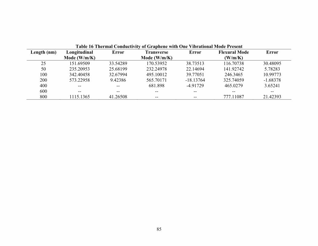
85

Table 16 Thermal Conductivity of Graphene with One Vibrational Mode Present Length (nm) Longitudinal

Mode (W/m/K) Error Transverse

Mode (W/m/K) Error Flexural Mode

(W/m/K) Error

25 151.69509 33.54289 170.53952 38.73513 116.70738 30.48095 50 235.20953 25.68199 232.24978 22.14694 141.92742 5.78283

100 342.40458 32.67994 495.10012 39.77051 246.3465 10.99773 200 573.22958 9.42386 565.70171 -18.13764 325.74059 -1.68378 400 -- -- 681.898 -4.91729 465.0279 3.65241 600 -- -- -- -- -- -- 800 1115.1365 41.26508 -- -- 777.11087 21.42393

REFERENCES

[1] S. Iijima, “Helical microtubules of graphitic carbon,” Nature, vol. 354, pp. 56–58, 1991.

[2] “Heat Transfer,” Heat Exchanger Design, 2011. [Online]. Available: http://heatexchanger-design.com/2011/03/07/heat-transfer-2/.

[3] C. Kittel and H. Kroemer, Thermal Physics, Second ed. W. H. Freeman, 1980. [4] J. Fourier, The Analytical Theory of Heat. London: Cambridge, 1878. [5] W. D. J. Callister, Materials Science and Engineering: An Introduction, 7th ed.

Wiley, 2006. [6] C. Kittel, Introduction to Solid State Physics, 8th ed. Wiley, 2004. [7] R. F. Pierret, Advanced Semiconductor Fundamentals, 2nd ed. Prentice Hall, 2002. [8] G. Chen, Nanoscale Energy Transport and Conversion: A Parallel Treatment of

Electrons, Molecules, Phonons, and Photons. Oxford University Press, USA, 2005. [9] W. S. Capinski, H. J. Maris, T. Ruf, M. Cardona, K. Ploog, and D. S. Katzer,

“Thermal-conductivity measurements of GaAs/AlAs superlattices using a picosecond optical pump-and-probe technique,” Phys. Rev. B, vol. 59, no. 12, p. 8105, Mar. 1999.

[10] S. Reich, C. Thomsen, and J. Maultzsch, Carbon Nanotubes: Basic Concepts and Physical Properties. Wiley-VCH, 2004.

[11] X. Lu and Z. Chen, “Curved Pi-Conjugation, Aromaticity, and the Related Chemistry of Small Fullerenes (,” Chem. Rev., vol. 105, no. 10, pp. 3643–3696, 2005.

[12] M. A. Osman and D. Srivastava, “Temperature dependence of the thermal conductivity of single-wall carbon nanotubes,” Nanotechnology, vol. 12, no. 1, pp. 21–24, 2001.

[13] J. Hone, M. Whitney, C. Piskoti, and A. Zettl, “Thermal conductivity of single-walled carbon nanotubes,” Phys. Rev. B, vol. 59, no. 4, p. R2514–R2516, Jan. 1999.

[14] D. J. Yang, Q. Zhang, G. Chen, S. F. Yoon, J. Ahn, S. G. Wang, Q. Zhou, Q. Wang, and J. Q. Li, “Thermal conductivity of multiwalled carbon nanotubes,” Phys. Rev. B, vol. 66, no. 16, p. 165440, Oct. 2002.

[15] J. Hone, M. C. Llaguno, N. M. Nemes, A. T. Johnson, J. E. Fischer, D. A. Walters, M. J. Casavant, J. Schmidt, and R. E. Smalley, “Electrical and thermal transport properties of magnetically aligned single wall carbon nanotube films,” Applied Physics Letters, vol. 77, no. 5, p. 666, 2000.

[16] P. Kim, L. Shi, A. Majumdar, and P. L. McEuen, “Thermal Transport Measurements of Individual Multiwalled Nanotubes,” Phys. Rev. Lett., vol. 87, no. 21, p. 215502, Oct. 2001.

[17] M. Fujii, X. Zhang, H. Xie, H. Ago, K. Takahashi, T. Ikuta, H. Abe, and T. Shimizu, “Measuring the Thermal Conductivity of a Single Carbon Nanotube,” Phys. Rev. Lett., vol. 95, no. 6, p. 065502, 2005.

[18] C. Yu, L. Shi, Z. Yao, D. Li, and A. Majumdar, “Thermal Conductance and Thermopower of an Individual Single-Wall Carbon Nanotube,” Nano Letters, vol. 5, no. 9, pp. 1842–1846, 2005.

86

[19] E. Pop, D. Mann, Q. Wang, K. Goodson, and H. Dai, “Thermal Conductance of an Individual Single-Wall Carbon Nanotube above Room Temperature,” Nano Letters, vol. 6, no. 1, pp. 96–100, Jan. 2006.

[20] J. P. Small, L. Shi, and P. Kim, “Mesoscopic thermal and thermoelectric measurements of individual carbon nanotubes,” Solid State Communications, vol. 127, no. 2, pp. 181–186, Jul. 2003.

[21] J. Hone, M. Whitney, and A. Zettl, “Thermal conductivity of single-walled carbon nanotubes,” Synthetic Metals, vol. 103, pp. 2498–2499, 1999.

[22] S. Berber, Y.-K. Kwon, and D. Tomanek, “Unusually High Thermal Conductivity of Carbon Nanotubes,” Phys. Rev. Lett., vol. 84, no. 20, p. 4613, May 2000.

[23] J. Che, T. Cagin, and W. A. Goddard III, “Thermal conductivity of carbon nanotubes,” Nanotechnology, vol. 11, no. 2, pp. 65–69, 2000.

[24] P. Kim, “Mesoscopic thermal transport and energy dissipation in carbon nanotubes,” Physica B: Condensed Matter, vol. 323, no. 1–4, pp. 67–70, Oct. 2002.

[25] S. Maruyama, “A molecular dynamics simulation of heat conduction in finite length SWNTs,” Physica B: Condensed Matter, vol. 323, no. 1–4, pp. 193–195, Oct. 2002.

[26] W. Zhang, Z. Zhu, F. Wang, T. Wang, L. Sun, and Z. Wang, “Chirality dependence of the thermal conductivity of carbon nanotubes,” Nanotechnology, vol. 15, no. 8, pp. 936–939, Aug. 2004.

[27] G. Zhang and B. Li, “Thermal conductivity of nanotubes revisited: Effects of chirality, isotope impurity, tube length, and temperature,” The Journal of Chemical Physics, vol. 123, no. 11, p. 114714, 2005.

[28] T. Y. Choi, D. Poulikakos, J. Tharian, and U. Sennhauser, “Measurement of thermal conductivity of individual multiwalled carbon nanotubes by the 3-ω method,” Applied Physics Letters, vol. 87, no. 1, p. 013108, 2005.

[29] M. Grujicic, G. Cao, and W. N. Roy, “Computational analysis of the lattice contribution to thermal conductivity of single-walled carbon nanotubes,” Journal of Materials Science, vol. 40, no. 8, pp. 1943–1952, 2005.

[30] T.-Y. Choi, D. Poulikakos, J. Tharian, and U. Sennhauser, “Measurement of the Thermal Conductivity of Individual Carbon Nanotubes by the Four-Point Three-ω Method,” Nano Lett., vol. 6, no. 8, pp. 1589–1593, 2006.

[31] M. C. Llaguno, “Thermal conductivity of single wall carbon nanotubes: Diameter and annealing dependence,” 2001, vol. 591, pp. 384–387.

[32] Z. L. Wang, D. W. Tang, X. B. Li, X. H. Zheng, W. G. Zhang, L. X. Zheng, Y. T. Zhu, A. Z. Jin, H. F. Yang, and C. Z. Gu, “Length-dependent thermal conductivity of an individual single-wall carbon nanotube,” Applied Physics Letters, vol. 91, no. 12, p. 123119, Sep. 2007.

[33] J. X. Cao, X. H. Yan, Y. Xiao, Y. Tang, and J. W. Ding, “Exact study of lattice dynamics of single-walled carbon nanotubes,” Phys. Rev. B, vol. 67, no. 4, p. 045413, Jan. 2003.

[34] J. X. Cao, X. H. Yan, Y. Xiao, and J. W. Ding, “Thermal conductivity of zigzag single-walled carbon nanotubes: Role of the umklapp process,” Phys. Rev. B, vol. 69, no. 7, p. 073407, Feb. 2004.

87

[35] C. W. Padgett and D. W. Brenner, “Influence of Chemisorption on the Thermal Conductivity of Single-Wall Carbon Nanotubes,” Nano Lett., vol. 4, no. 6, pp. 1051–1053, Jun. 2004.

[36] R. Saito, R. Matsuo, T. Kimura, G. Dresselhaus, and M. S. Dresselhaus, “Anomalous potential barrier of double-wall carbon nanotube,” Chemical Physics Letters, vol. 348, no. 3–4, pp. 187–193, Nov. 2001.

[37] W. Guo and Y. Guo, “Energy Optimum Chiralities of Multiwalled Carbon Nanotubes,” Journal of the American Chemical Society, vol. 129, no. 10, pp. 2730–2731, Mar. 2007.

[38] E. Mamontov, C. J. Burnham, S.-H. Chen, A. P. Moravsky, C.-K. Loong, N. R. de Souza, and A. I. Kolesnikov, “Dynamics of water confined in single- and double-wall carbon nanotubes,” The Journal of Chemical Physics, vol. 124, no. 19, p. 194703–194703–6, May 2006.

[39] M. Dequesnes, S. V. Rotkin, and N. R. Aluru, “Calculation of pull-in voltages for carbon-nanotube-based nanoelectromechanical switches,” Nanotechnology, vol. 13, no. 1, pp. 120–131, Feb. 2002.

[40] S. U. S. Choi, Z. G. Zhang, W. Yu, F. E. Lockwood, and E. A. Grulke, “Anomalous thermal conductivity enhancement in nanotube suspensions,” Appl. Phys. Lett., vol. 79, no. 14, p. 2252, 2001.

[41] M. J. Biercuk, M. C. Llaguno, M. Radosavljevic, J. K. Hyun, A. T. Johnson, and J. E. Fischer, “Carbon nanotube composites for thermal management,” Appl. Phys. Lett., vol. 80, no. 15, p. 2767, 2002.

[42] H. Xie, H. Lee, W. Youn, and M. Choi, “Nanofluids containing multiwalled carbon nanotubes and their enhanced thermal conductivities,” Journal of Applied Physics, vol. 94, no. 8, p. 4967, 2003.

[43] S. T. Huxtable, D. G. Cahill, S. Shenogin, L. Xue, R. Ozisik, P. Barone, M. Usrey, M. S. Strano, G. Siddons, M. Shim, and P. Keblinski, “Interfacial heat flow in carbon nanotube suspensions,” Nature Materials, vol. 2, no. 11, pp. 731–734, Oct. 2003.

[44] A. Moisala, Q. Li, I. A. Kinloch, and A. H. Windle, “Thermal and electrical conductivity of single- and multi-walled carbon nanotube-epoxy composites,” Composites Science and Technology, vol. 66, no. 10, pp. 1285–1288, Aug. 2006.

[45] C.-W. Nan, Z. Shi, and Y. Lin, “A simple model for thermal conductivity of carbon nanotube-based composites,” Chemical Physics Letters, vol. 375, no. 5–6, pp. 666–669, Jul. 2003.

[46] F. H. Gojny, M. H. G. Wichmann, B. Fiedler, I. A. Kinloch, W. Bauhofer, A. H. Windle, and K. Schulte, “Evaluation and identification of electrical and thermal conduction mechanisms in carbon nanotube/epoxy composites,” Polymer, vol. 47, no. 6, pp. 2036–2045, Mar. 2006.

[47] A. A. Balandin, S. Ghosh, W. Bao, I. Calizo, D. Teweldebrhan, F. Miao, and C. N. Lau, “Superior Thermal Conductivity of Single-Layer Graphene,” Nano Lett., vol. 8, no. 3, pp. 902–907, 2008.

[48] P. G. Klemens, “Theory of the A-Plane Thermal Conductivity of Graphite,” Journal of Wide Bandgap Materials, vol. 7, no. 4, pp. 332–339, Apr. 2000.

[49] P. G. Klemens, “Theory of Thermal Conduction in Thin Ceramic Films,” Internation Journal of Thermophysics, vol. 22, no. 1, p. 265–175, 2001.

88

[50] D. L. Nika, E. P. Pokatilov, A. S. Askerov, and A. A. Balandin, “Phonon thermal conduction in graphene: Role of Umklapp and edge roughness scattering,” Phys. Rev. B, vol. 79, no. 15, p. 155413, Apr. 2009.

[51] D. L. Nika, S. Ghosh, E. P. Pokatilov, and A. A. Balandin, “Lattice thermal conductivity of graphene flakes: Comparison with bulk graphite,” Applied Physics Letters, vol. 94, no. 20, p. 203103–203103–3, May 2009.

[52] “Grüneisen parameter.” [Online]. Available: http://en.wikipedia.org/wiki/Gr%C3%BCneisen_Parameter. [Accessed: 17-Feb-2012].

[53] J. Hu, X. Ruan, and Y. P. Chen, “Thermal Conductivity and Thermal Rectification in Graphene Nanoribbons: A Molecular Dynamics Study,” Nano Lett., vol. 9, no. 7, pp. 2730–2735, 2009.

[54] Z. Guo, D. Zhang, and X.-G. Gong, “Thermal conductivity of graphene nanoribbons,” Applied Physics Letters, vol. 95, no. 16, p. 163103–163103–3, Oct. 2009.

[55] S. Ghosh, I. Calizo, D. Teweldebrhan, E. P. Pokatilov, D. L. Nika, A. A. Balandin, W. Bao, F. Miao, and C. N. Lau, “Extremely high thermal conductivity of graphene: Prospects for thermal management applications in nanoelectronic circuits,” Applied Physics Letters, vol. 92, no. 15, p. 151911–151911–3, Apr. 2008.

[56] P. Zhang, Y. Huang, P. H. Geubelle, P. A. Klein, and K. C. Hwang, “The elastic modulus of single-wall carbon nanotubes: a continuum analysis incorporating interatomic potentials,” International Journal of Solids and Structures, vol. 39, no. 13–14, pp. 3893–3906, Jun. 2002.

[57] S. J. Stuart, A. B. Tutein, and J. A. Harrison, “A reactive potential for hydrocarbons with intermolecular interactions,” J. Chem. Phys., vol. 112, no. 14, p. 6472, 2000.

[58] J. Tersoff, “New empirical approach for the structure and energy of covalent systems,” Phys. Rev. B, vol. 37, no. 12, p. 6991, Apr. 1988.

[59] D. W. Brenner, “Empirical potential for hydrocarbons for use in simulating the chemical vapor deposition of diamond films,” Phys. Rev. B, vol. 42, no. 15, p. 9458, Nov. 1990.

[60] F. Muller-Plathe, “A simple nonequilibrium molecular dynamics method for calculating the thermal conductivity,” The Journal of Chemical Physics, vol. 106, p. 6082, 1997.

[61] F. Muller-Plathe and D. Reith, “Cause and effect reversed in non-equilibrium molecular dynamics: an easy route to transport coefficients,” Computational and Theoretical Polymer Science, vol. 9, no. 3–4, pp. 203–209, Dec. 1999.

[62] S. J. Plimpton, “Fast Parallel Algorithms for Short-Range Molecular Dynamics,” J Comp Phys, vol. 117, pp. 1–19, 1995.

[63] J. T. Frey and D. J. Doren, TubeGen. Newark, DE: University of Delaware, 2005. [64] H. A. Rafizadeh, “An analytical-potential approach to the lattice dynamics of

graphite,” Physica, vol. 74, no. 1, pp. 135–150, May 1974. [65] L. Lindsay and D. A. Broido, “Optimized Tersoff and Brenner empirical potential

parameters for lattice dynamics and phonon thermal transport in carbon nanotubes and graphene,” Phys. Rev. B, vol. 81, no. 20, p. 205441, May 2010.

89

90

[66] L. Lindsay, D. A. Broido, and N. Mingo, “Diameter dependence of carbon nanotube thermal conductivity and extension to the graphene limit,” Phys. Rev. B, vol. 82, no. 16, p. 161402, Oct. 2010.

[67] E. González Noya, D. Srivastava, L. A. Chernozatonskii, and M. Menon, “Thermal conductivity of carbon nanotube peapods,” Phys. Rev. B, vol. 70, no. 11, p. 115416, 2004.

[68] M. G. Holland, “Analysis of Lattice Thermal Conductivity,” Phys. Rev., vol. 132, no. 6, pp. 2461–2471, Dec. 1963.

[69] J. Callaway, “Model for Lattice Thermal Conductivity at Low Temperatures,” Phys. Rev., vol. 113, no. 4, pp. 1046–1051, Feb. 1959.

[70] E. A. Walker and D. G. Walker, “Influence of Vibrational Modes on Thermal Conductivity in Single-walled Carbon Nanotubes,” Submitted for Publication.

EBONEE ALEXIS WALKER Dissertation Submitted to...

Documents

Transcript of EBONEE ALEXIS WALKER Dissertation Submitted to...