Easing the challenge of RF design

Designing in a wireless link needn’t be a nightmare if you follow some simple guidelines. Jay Tyzzer explains

(Note: Blue font indicates text reproduced on website.) The very mention of RF design is usually enough to scare all but the most confident designer. However, wireless specialists such as the company I work for, Nordic Semiconductor, have worked hard to ensure it’s no longer solely the domain of the RF expert. Performance optimised transceivers, and the availability of development kits and reference layouts, makes it possible for a competent electronics design engineer to incorporate wireless hardware into their latest product. Nonetheless, although the availability of commercial off-the-shelf (COTS) components and reference designs has made wireless system design a little easier, the engineer still needs to acquire some fundamental knowledge about the parameters that influence a wireless link’s performance. A critical issue is communication reliability; how will parameters such as sensitivity, output power, adjacent channel selectivity and operating frequency influence system performance? In other words, what is the probability of transmitting/receiving an error free data packet in the presence of other radio sources that could interfere with the signal. A second equally critical issue is range. The designer has to ensure that the radio can operate over its stated range in a number of different operating environments. Given output power and sensitivity, what other parameters affect range? Environmental factors such as air humidity, obstacles such as people and furniture, building materials and metal film sun-screened windows limit useful range and choice of antenna implementation. The designer should also be very wary of taking the data sheets of some wireless component vendors as gospel. For example, if sensitivity is measured for a lower data-rate than the stated maximum then it’s worth asking why. Checking just a few fundamental characteristics such as these first may save much time and frustration later when realising that the circuit chosen does not comply with the system specifications. Fundamentals of a wireless link A wireless link comprises a transmitter with antenna, a transmission path and a receiver with antenna. The key performance parameters of this simple link are the output power (Pout) of the transmitter and the sensitivity of the receiver (see figure 1).

Figure 1: Schematic of a typical point-to-point wireless link Sensitivity is the minimum received power that results in a satisfactory Bit Error Rate (BER, usually 10-

3 or one bit error for every 1000 bits transferred at the received data output (i.e. correctly demodulated)) or Packet Error Rate (PER, see sidebar “The importance of Packet Error Rate”).

The difference between received signal power and the receiver sensitivity limit is the transmission link margin or “headroom”. Headroom is reduced by a number of factors such as transmission path length, antenna efficiency, carrier frequency and obstructions in the transmission path (see figure 2).

Figure 2: Headroom is reduced by a number of factors such as transmission path length, antenna efficiency and obstructions in the transmission path Note that sensitivity and output power quoted in the RF-circuit datasheets are given for the load impedance optimised for the input low noise amplifier (LNA) and the output power amplifier. This means that the impedance of the antenna must be equal to the load stated in the datasheet, otherwise a mismatch and subsequent loss of headroom occurs. A typical matching network introduces around 1 to 3dB of attenuation.    The antenna transforms the transmitter output power into electromagnetic energy, which radiates from the antenna in a radiation pattern determined by the antenna geometry. For the licence free bands such as 915MHz in the US, 434 and 868MHz in Europe, and the global 2.4 GHz band, the maximum output power is expressed as Effective Isotropic Radiated Power (EIRP). An “isotropic radiator” is defined as a hypothetical lossless antenna radiating equally in all directions. This means the regulations governing the licence-free bands (issued by ETSI) do not allow transmission range to be boosted by using a directional antenna. If the antenna gain is larger than 1 (0dB) in any given direction, the output power has to be decreased accordingly. For example, for a radio operating in the 2.4GHz band, the maximum transmission power is 25mW (14dBm) EIRP. A directional antenna that has 10dB gain in a given direction would seem as if it was transmitting 24dBm for a receiver positioned in this direction. Thus, the output power would have to be reduced to 4dBm to fulfil the ETSI requirements. Note that a directional antenna can be used for receivers without any penalty. Calculating antenna gain and radiation pattern is generally quite complex, and its local environment heavily influences the resulting radiation pattern. Placing the antenna close to conducting surfaces is likely to distort the antenna’s radiation pattern and efficiency, but is virtually unavoidable for most practical applications. Calculating antenna size The antenna’s ability to transform the output power into radiated energy is represented by the

parameter Gant. Antenna gain is generally proportional to physical size, in accordance with the following formula from antenna theory: Gant = (4 . π . Ae)/ λ2 where Ae is the effective area of the antenna and λ is the wavelength of the carrier frequency. For the 2.4GHz band, the wavelength is approximately 0.125m. From the formula, the necessary effective area to achieve an antenna gain of 1 (0dB) is 0.00124m2 (12.4 by 12.4cm). For most practical applications an antenna this size would be too voluminous and cumbersome, so designers settle on something a bit smaller. Many designers opt for a so-called quarter wave antenna because it is the smallest practical antenna for portable 2.4GHz designs. The theoretical length of a quarter wave antenna would be λ/4, or 3.125cm. A popular small, low-cost antenna for low power radio applications – often called a “meandering” or “crank-like antenna” (CLA) - forms part of the PCB and does not represent a significant cost other than PCB area. The ratio of the length of the antenna to its diameter together with other variables such as the PCB substrate may affect the final antenna length. A CLA is usually a little longer than a quarter wave antenna and the CLA’s performance is dependent on its geometry and relationship to the PCB’s ground plane. It is suggested that the designer starts with an antenna slightly longer than calculated and then shortens it until resonance occurs. Figure 3 shows the antenna on the PCB used for the dongle of Nordic’s nRF24LU1+ compact USB reference design. This antenna has a typical efficiency (or gain) of approximately -20 to -25dB. Notice that by making the antenna much smaller than the unity gain dimensions (12.4 by 12.4cm) the gain is diminished. Consequently, the antenna typically represents a loss in the transmission “budget”.

Figure 3: Meandering type antenna (extreme right of PCB) of Nordic’s nRF24LU1 compact USB reference design The transmitter radiates power uniformly in all directions (assuming the antenna is isotropic as discussed above) forming a sphere. Consequently, at a distance r from the antenna, the power density (or “flux”) decreases by an amount proportional to 1/r2 as it spreads out in a sphere of increasing surface area. The actual equation that determines the Flux density (F) at a distance r from the transmitter is: F = (Pout . Gant_TX)/( 4 . π . r2) [W/m2] The received power at the receiver is: Prec = (Pout_TX . Gant_TX . Gant_RX)/Path_loss Where Path_loss = (4 . π . r/ λ )2 In other words, both range and transmission frequency determines the Path_loss. For the receiver to demodulate, the received power must be equal to, or larger than the sensitivity limit (see figure 1). In ideal conditions, a 6dB (fourfold) increase in output power (or receiver sensitivity) corresponds to a doubling of the effective range. Headroom decreases with range, and as headroom is reduced, the probability of communication loss due to environmental obstacles increases. For example, if the headroom of a 2.4GHz link is less than

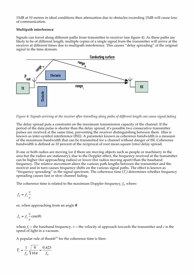
15dB at 10 metres in ideal conditions then attenuation due to obstacles exceeding 15dB will cause loss of communication. Multipath interference Signals can travel along different paths from transmitter to receiver (see figure 4). As these paths are likely to be of different length, multiple copies of a single signal from the transmitter will arrive at the receiver at different times due to multipath interference. This causes “delay spreading” of the original signal in the time domain.

Figure 4: Signals arriving at the receiver after travelling along paths of different length can cause signal fading The delay spread puts a constraint on the maximum transmission capacity of the channel. If the period of the data pulse is shorter than the delay spread, it’s possible two consecutive transmitter pulses are received at the same time, preventing the receiver distinguishing between them (this is known as inter-symbol interference (ISI)). A parameter known as coherence bandwidth is a measure of the maximum bandwidth that can be transmitted for a channel without danger of ISI. Coherence bandwidth is defined as 10 percent of the reciprocal of root mean square (rms) delay spread. If one or both radios are moving (or if there are moving objects such as people or machinery in the area but the radios are stationary), due to the Doppler effect, the frequency received at the transmitter can be higher (for approaching radios) or lower (for radios moving apart) than the baseband frequency. The relative movement alters the various path lengths between the transmitter and the receiver and in turn causes frequency shifts on the various signal paths. The effect is known as “frequency spreading” in the signal spectrum. The coherence time (Tc) determines whether frequency spreading causes fast or slow channel fading. The coherence time is related to the maximum Doppler frequency, fd, where:

€

fd = fovc

or, when approaching from an angle θ

€

fd = fovccos(θ)

where fo = the baseband frequency, v = the velocity of approach towards the transmitter and c is the speed of light in a vacuum. A popular rule of thumb(1) for the coherence time is then:

€

Tc =1fd

916π

=0.423fd

Slow channel fading occurs when the coherence time is large compared with the signal pulse period. For slow channel fading the amplitude and phase change exhibited by the channel can be considered roughly constant over the period of use. Fast channel fading occurs when the coherence time of the channel is small relative to the signal pulse period. This presents challenges for wireless protocols with long packet lengths if the relative velocity between transmitter and receiver is large. In fast channel fading the amplitude and phase change exhibited by the channel varies rapidly over the period of use. Fast fading manifests itself as signal strength dips that can have a magnitude of several tens of decibels even in close vicinity to the transmitter. Multipath interference is caused by reflection, diffraction and scattering. Reflection occurs when the transmitted energy reflects off the surface of an object that is large compared to the carrier wavelength (for example, walls, buildings or the ground). Diffraction describes the “wave-bending” around sharp irregular edges of an object in the transmission path. Scattering describes energy dispersion, caused by objects that are small compared to the wavelength of the propagating wave. The loss depends heavily on the physical characteristics of the object. A designer must be prepared for the multipath interference caused by obstacles such as floors, walls, buildings and windows. For example, reinforced concrete walls introduce higher losses than wooden or plaster walls. Metal tinted windows are high loss barriers compared to un-tinted windows (see table 1). Furthermore, a designer must be aware of the coherence time of his radio system if it’s likely that the receiver and transmitter are moving relative to each other when in use.

Table 1: Attenuation due to common building materials

Consider a 2.4GHz system with 10dBm output power, antenna efficiency (gain) of -20dB and -105dBm sensitivity. This system may have a theoretical range of more than 40 metres, but in a typical application – taking into account multipath interference, coherence bandwidth and coherence time - the effective range may drop to just 5 to 10 metres. This is why the designer should treat a manufacturer’s “free-line-of-sight” range with caution. Know your parameters Designing a radio system requires knowledge of some fundamental parameters to understand what will influence link performance and reliability. I have already discussed perhaps the most fundamental parameters; output power and receiver sensitivity. The others that are important are listed here:

• Receiver dynamic range; • Co-channel rejection; • Adjacent channel selectivity; • Reference frequency stability; • Mirror image attenuation; • Modulation principle • Intermodulation performance.

These are all important parameters that, although not directly part of the transmission budget, do have an affect on transmission reliability, especially when other transmitters are in close proximity. So, having established the transmission budget, the next question a designer should ask is: “How does my system behave when an unrelated transmitter radiates energy into the local environment?”

To answer that question, the designer must consider each of the parameters in turn. The receiver dynamic range is the maximum power variation at the receiver input pins that still results in a correctly demodulated signal. This means that to be received properly, the power of the signal of interest must be between the sensitivity limit and the sensitivity limit plus the dynamic range. The co-channel rejection (CCR) is a measure of the capability of the receiver to demodulate a “wanted” modulated signal without exceeding a given degradation due to the presence of an “unwanted” modulated signal, when both signals are at the same nominal frequency. This parameter is specified in decibels. For example, a co-channel rejection of 10dB would mean that if the wanted signal is 10dB (or higher) than the unwanted signal, then correct demodulation will occur (with a typical BER of less than 10-3). If this parameter is not specified in the datasheet, then a designer should assume 12 to 14dB co-channel rejection (the typical Frequency Shift Keying (FSK) demodulator threshold (see below)). As an example, consider the system in figure 5, with two adjacent transmitters operating at the same frequency. Let’s calculate how far away the unwanted signal source needs to be so as not to interfere with the demodulation of the wanted signal.

Figure 5: Schematic of adjacent transmitters operating at the same nominal frequency

The equation for received power is: (Pout1 . Gant1 . Gant_RX)/Path_loss1 > ((Pout2 . Gant2 . Gant_RX)/Path_loss1) . CCR Can be reduced to: Pout1 – Pout2 +20 . log(range2/range1) > CCR Assuming a CCR of 12dB, and that the transmitters have equal output power and antenna gain, the ratio between range2 and range1 must be at least 4 in order for the receiver to demodulate the wanted TX1 signal correctly without interference from TX2. The adjacent channel selectivity (ACS) of the receiver is defined by the European Telecommunications Standards Institute (ETSI), for example, as the ability of a receiver to demodulate a received signal at the sensitivity limit, in the presence of a sine component centred in the adjacent channel (see figure 6). (I.e. if the ACS for a 25kHz channel system is given as 30dB, demodulation of the wanted signal at the sensitivity limit may be performed with a sine component of 30dB higher power than the received signal present in the adjacent channel.)

Figure 6: The ACS of the receiver is a measure of the ability to demodulate a received signal at the sensitivity limit, in the presence of a sine component of an unwanted signal centred in the adjacent channel Note that the ETSI definition is merely provided as a comparative figure. The system ACS is typically lower, as the signal in the adjacent channel is unlikely to be a sine component, rather a modulated spectrum. Reference frequency stability is a parameter that influences ACS. Deviation from the ideal crystal reference frequency will result in a corresponding deviation of the transmitted frequency, and an intermediate frequency (IF) offset/deviation for a superheterodyne receiver (one that shifts the received signal to an IF) appearing as an offset in the IF-filter centre frequency (see figure 7). Receivers use the superheterodyne principle for its excellent channel filtering performance, but suppression is needed to avoid mirror image interference. Mirror image attenuation (MIA) is a measure of the extent of this suppression. In figure 7 the mirror image is shown positioned at the local oscillator (LO)-frequency minus the IF, but will also appear at the IF together with the wanted signal. Consequently the mirror image frequency must be attenuated to avoid destructive disturbance or loss of sensitivity.

Figure 7: Deviation from the crystal reference frequency results in a corresponding deviation of the transmitted frequency, and an intermediate frequency (IF) offset/deviation appearing as an offset in the IF-filter centre frequency MIA has traditionally been performed with an external filter at the antenna input, or more recently, with on-chip cancellation techniques. As the mirror image appears inside the IF-filter bandwidth after mixing, MIA minus CCR is the maximum allowable power difference between the two signals to ensure demodulation. For example, if the mirror image attenuation is 35dB and the co-channel rejection is 12dB, the received mirror image frequency power may not be higher than 23dB (i.e. 35dB -12dB) compared to the wanted signal.

In the early days (particularly in the 433MHz band), amplitude shift keying (ASK, also known as on-off keying or OOK) was the dominant modulation principle in the license-free low power radio bands. Unfortunately, although ASK-based transceivers are simple and reasonably priced, they suffer from relatively poor reliability when under the influence of in-band interference. In ASK systems, logic ’1’ is represented by a carrier frequency, while logic ’0’ is represented by no carrier. Consequently, the presence of a very weak unwanted signal in the channel can be interpreted as logic ’1’ if the receiver is sufficiently sensitive. Frequency Shift Keying (FSK) is a different approach in which each the two logic levels correspond to a frequency value; DATAFSK = “1” → f’1’ = fcentre + ∆f DATAFSK = “0” → f’0’ = fcentre - ∆f The technique ensures that the receiver always sees a strong signal swamping any unwanted signal in the channel. Gaussian Frequency Shift Keying (GFSK) and Gaussian Minimum Shift Keying (GMSK - the term used for a GFSK signal in which the bit rate is four times the frequency deviation) modulation are enhanced versions of FSK implemented to optimise modulation bandwidth efficiency (i.e. the maximum transmitted number of bits per Hertz of channel bandwidth). GFSK applies Gaussian filtering to the modulated baseband signal before it is applied to the carrier. This results in a “dampened” or gentler frequency swing between the high (“1”) and low (“0”) levels. The result is a narrower and “cleaner” spectrum for the transmitted signal compared with the straightforward approach of FSK. Figure 8 shows the general principle.

Figure 8: General principle of GSFK Intermodulation performance is a measure of how well a receiver supresses intermodulation products. Intermodulation products are artifacts that result because a superheterodyne receiver’s output is not a linear function of its input. In the frequency domain the products appear at the harmonic frequencies of the primary frequency f1 (i.e. 2f1, 3f1 etc.). These are little problem because they generally occur outside of the radio’s passband. Of greater concern are intermodulation products resulting from a receiver handling two different frequencies (for example, in the mixer stage of a superheterodyne receiver). In this case the problem is due to odd-order intermodulation products occurring at frequencies much closer to the primary

frequencies and therefore inside the radio’s passband. Consider the following example: f1 = 2.46GHz, f2 = 2.47GHz Then the third order products occur at 2f1 - f2 = 2.45GHz and 2f2 - f1 = 2.48GHz The fifth order products occur at 2.44GHz and 2.49GHz. It can be seen that these intermodulation products are very close to the principal frequencies. Consequently, if the transceiver’s intermodulation performance is substandard, the products will be poorly suppressed and will cause significant signal distortion and loss of sensitivity. Also note that if the products are generated and amplified by a substandard transmitter they can interfere with nearby receivers even though the rogue transmitter is nominally transmitting on a different frequency – something that won’t be popular when the emphasis is on co-existence in the crowded 2.4GHz band. Avoiding interference

As more companies produce products that use the licence-free portion of the low power radio spectrum, designers have to deal with the possibility of interference from radio signals from other sources operating on an identical (or at least very close to) their own chosen operating frequency. In fact, regulations governing the ISM parts of the spectrum state “a device must expect interference”.

There are three basic techniques for minimising the impact of interference for devices operating in the 2.4GHz band. These are Time Domain Multiple Access (TDMA), Direct Sequence Spread Spectrum (DSSS) and Frequency Hopping Spread Spectrum (FHSS).

TDMA works by subdividing narrowband allocations within the ISM portion of the spectrum into a number of timeslots allowing several users to share the same single frequency without danger of clashing. Each transceiver waits for its own clear timeslot before transmitting, thus avoiding interference. DSSS and FHSS both rely on modulation of the carrier signal. In addition, FHSS allocates a number of channels within the band, the exact width of which depends on the technology (see below).

Figure 9: ANT’s TDMA-like interference scheme subdivides a narrow frequency band into timeslots. A single timeslot comprises a guard band, followed by a short transmission, followed by another guard band. Nodes 1, 2 and 3 adapt transmissions so that no clashes occur. If required, the system can switch frequencies to accommodate additional timeslots (Nodes A, B and C)

In simple terms, DSSS transmissions multiply the data being transmitted by a “noise” component. This noise signal is a pseudorandom sequence at a frequency much higher than that of the original 2.4GHz signal, thereby spreading the energy of the original signal across a much wider band. The noise is filtered out at the receiving end to recover the original data, by again multiplying the same pseudorandom sequence by the received signal.

For de-spreading to work correctly, transmit and receive sequences must be synchronised. This requires the receiver to ‘lock’ its sequence with the transmitter’s via a timing search process. DSSS operates at the cost of transmitting excessive data packets, incurring extra bandwidth usage and current consumption overheads.

Using FHSS, a wireless technology periodically retunes to a different channel in a pre-defined (determined by a look up table) or pseudo-random sequence. Bluetooth wireless technology, for example, uses FHSS in conjunction with GFSK, splitting the 2.4GHz ISM band into 79 x 1MHz channels (with a 1MHz guard channel at the lower end of the band and a 2MHz guard channel at the higher end). Transmitting and receiving Bluetooth wireless technology devices then hop between the 79 channels 1600 times per second in a pseudo-random pattern.

From Bluetooth 1.2 on, a revised form of frequency hopping is used, dubbed adaptive frequency hopping (AFH). This algorithm allows Bluetooth wireless technology devices to mark channels as good, bad, or unknown. Bad channels in the frequency-hopping pattern are then replaced with good channels via a look-up table.

Nordic’s Frequency Agility Protocol (FAP) uses a simplified frequency hopping scheme in that the transmitting and receiving pair establish communication on a particular frequency and then only hop to a different frequency should interference be experienced. The channel on which the interference was experienced is marked and not reused during that particular communication cycle.

In its 2.4GHz variant, ZigBee uses 16 channels at 5MHz spacing; each channel occupies 3MHz, giving a 2MHz gap between pairs of channels. ZigBee then uses a simple DSSS scheme for data transmission.

Devices such as Nordic’s nRF24AP2 used in very low duty cycle applications such as sports-based heart rate monitoring and wireless transmission to a watch-based recorder – employ a proprietary form of TDMA developed by Nordic’s design partner ANT. The nRF24AP2’s TDMA-like collision avoidance approach relies on each transceiver transmitting in a clear timeslot. If there are a number of discrete systems working side-by-side – such as a row of rowing machines all lined up next to each other in a gym – then by “listening” for drifting transmission sources on its frequency the wireless node can determine if there is approaching interference and adapt its transmissions accordingly (see figure 9).

Interpreting the datasheet As a systems designer, a key requirement is to have clear information about circuit performance that can be used to make comparative assessments between the various RF-IC alternatives. Although datasheets are supposed to help in this respect, this is not always the case. A highly competitive market has led to some ingenious ways of rewriting parameter definitions in order to make circuit performance look better than it actually is. Consequently, there is a need for caution when reading and using the parameters given in datasheets. Some knowledge of “the not-so-fine art of creative RF-datasheet writing” may be in order. For example, if the measurement conditions of one or more of the key parameters are not given, try to find out why. (The manufacturer may have chosen to be “economical with facts” by omitting the details.) Start by verifying the data rate. Terms such as “data rate”, “chip rate” and “baud rate” are all used to describe the amount of data transferred per unit time by the transceiver. Make sure you understand how the silicon vendor defines this parameter. The transceiver needs to meet your requirement of the data you wish to transfer when employing your designated protocol (this is not necessarily the same as the “raw” data rate). Next, consider the sensitivity. This is an important parameter when calculating the transmission link budget (see section entitled “Fundamentals of a wireless link” above). In systems where multiple data rates and IF-filter bandwidths exist, make sure that the sensitivity given is for the maximum data rate (or, at least, the data rate you wish to use). Generally, sensitivity drops with IF-filter bandwidth. Note that some manufacturers are pushing for Packet Error Rate (as well as BER) to be included as a reference sensitivity measurement (see sidebar “The importance of Packet Error Rate”). Then make sure that the ACS is given for the adjacent channel and not further away from the receiver channel. Stating the “ACS” for a frequency further away from the received channel than the channel spacing is bound to improve this parameter. Some vendors state “adjacent channel attenuation” (ACA) which is not the same as ACS. ACA only states the attenuation of a signal at a given spacing from the received channel, not how large this signal may be before demodulation is inhibited. Generally ACS is lower than the ACA. Current consumption is important, particularly for ultra-low power (ULP) applications (for example, those using coin cell batteries such as the 3V, 180 to 220mAh-capacity CR2032 type that can only support a peak load 20mA). Be sure that the current consumption is given for the frequency band in which you intend to use the device. It also important to determine the peak currents when transmitting and receiving, plus currents when the transceiver is in “sleep” or other power down modes. While peak currents are obviously important, battery capacity can be significantly affected if the transceiver spends long periods in other modes. Next, consider the crystal requirement. This parameter is usually stated as the maximum allowed offset from the nominal frequency in parts per million (ppm). Make sure that the requirement stated in the datasheet is valid for the channel bandwidth and frequency deviation used. Some transceiver solutions are based upon receiver tracking of the received signal in order to reduce

crystal reference requirements. In other words, the receiving frequency is actively adjusted in order to “find” the transmitted signal. Note that the transmitted frequency will still drift according to the transmitter crystal offset. Although this approach will ensure communication between two units, transmitter frequency drift must still comply with the channel spacing of the system. For example, trying to use a ±20ppm crystal for a 2.4GHz system with 25kHz channel spacing will result in a worse case transmitter frequency drift of 48kHz. Generally the crystal reference is a significant part of the total system cost. Also note that crystal cost is proportional to the temperature range over which specified performance is guaranteed. The crystal’s load capacitance (CL) will also significantly affect the systems start-up time and start-up power consumption (and important consideration in ultra-low power applications). A lower CL reduces the start-up time, but increases start-up power consumption. Care should be taken to find the best compromise between the two. The crystal manufacturer normally specifies the device’s CL value. The following formula matches the crystal’s CL with the proper loading capacitors: C = 2(CL) – (CP + CI) Where C is the unknown value of the load capacitor, CL is the known value from the crystal manufactures datasheet, CP is the parasitic capacitance in the circuit (from traces, wires etc.) and CI is the input capacitance of the device itself. The CP + CI value is usually between 2 and 5. For radios from Nordic Semiconductor, a typical value is 2pf. Therefore, for a crystal with a CL of 12pf: C = 2(12) -2 = 22pf. However, sometimes the result is a non-standard capacitance value. In that case, moving up or down a few picofarads to a standard value usually allows the system to operate satisfactorily. Moreover, proper layout protocol can lower the value of CP. Finally, consider the switching time between different operational modes (For example, transmit to receive mode and power-down to receive mode). Remember to add the duration time of “training” - or preamble sequences. Some receiver topologies require lengthy “10101010...”-sequences in order to initialise or synchronise the demodulator. Moreover, the receiver frequency tuning sequences described in the crystal reference section (above), is generally time-consuming compared to the given switching time. Designing a low power radio wireless link with good range and reliable communication is well within the capabilities of a competent electronics engineer, provided they take time to understand the electronic, physical and environmental factors that affect RF performance. However, partnering with an expert such as Nordic Semiconductor considerably eases the task. Nordic specialises in ULP short-range wireless connectivity and produces complete silicon solutions including class-leading 2.4GHz single chip transceivers, development tools, application specific communication software and reference designs. The company’s range of nRF24xx range of 2.4GHz transceivers are aimed at applications such as PC peripherals – for example, wireless keyboards/mice - game controllers, intelligent sports equipment and wireless audio (for example, mp3 and portable CD player headphones and PC speakers). About the Author: Jay Tyzzer is a senior applications engineer with Nordic Semiconductor based on the US West Coast. Further information: This feature is based on a white paper by Frank Karlsen, an RF Designer with Nordic Semiconductor, entitled “Guidelines to low cost wireless system design”. The white paper can be downloaded from www.nordicsemi.com.

REFERENCE 1. “Wireless Communications: Principles & Practice”, Theodore S Rappaport, Prentice Hall, 2002 SIDEBAR

The importance of Packet Error Rate

Bit Error Rate (BER) is an important measure of the integrity of a radio link. But for a fixed BER, Packet Error Rate (PER) will increase as the packet length increases. This factor is particularly important for systems where the developer is able to change the packet length (for example, as with Nordic Semiconductor’s nRF24xxx 2.4GHz transceivers).

Transceiver manufacturers have pushed for PER to be included as a reference sensitivity measurement so that developers are aware that a significant number of packets could be lost even if the BER is below 10-3.

Consider the following example: Assume a BER of 10-3 or one bit error for every 1000 bits transferred at the received data output. Also assume that bit errors are randomly distributed with a rectangular error probability density function and that bit errors are not correlated. The probability of a particular bit being correct at a BER of 10-3 is 0.999 For a typical ultra-low power (ULP) 2.4GHz transceiver packet configuration a bit error has the following effect: Preamble (8 bit): Packet can be recovered Sync word (32 bit): Error, packet is lost Packet type field (16 bit): Error, packet is lost Payload (296 bit): Error, packet is lost CRC (24 bit); Error, packet is lost The number of significant bits in an ULP test packet is thus 368 bits (out of a total of 376 bits) The probability of a 368 bit sequence containing no bit errors is = 0.999368 = 0.692 Resulting PER = (1 - 0.692) × 100 percent = 30.8 percent. In other words for a 376 bit packet with 368 significant bits transmitted at a BER of 10-3, nearly one in three packets is lost. If, for example, the payload is halved (to 148 bits) the PER drops to one in five packets (for the same BER). DOCUMENT ENDS © NORDIC SEMICONDUCTOR 2010, www.nordicsemi.com