EARTHQUAKE MAGNITUDE, INTENSITY, ENERGY,

POWER LAW RELATIONS AND SOURCE MECHANISM

J.R. Kayal

Geological Survey of India, 27, J.L. Nehru Road Road, Kolkata – 700 016 email : jr_kayal@hotmail.com

EARTHQUAKE MAGNITUDE

Magnitude is one of the basic and important parameters of an earthquake. It defines the size of an earthquake. The beginners of seismology are, in general, confused about different scales of magnitude, and sometimes they mix-up earthquake intensity with its magnitude. Journalists often report the magnitude value of an earthquake as its intensity; this is wrong.

There are now different magnitude scales to define the size of an earthquake. After Richter (1935), various magnitude scales are proposed; all these scales are discussed below.

Richter Magnitude (or Local Magnitude) ML

Richter (1935) defined the local magnitude ML of an earthquake observed at a station to be

ML = log A - log Ao ( ∆) (1) where A is the maximum amplitude in millimetres recorded on the Wood-Anderson seismograph for an earthquake at epicentral distance of ∆ km, and Ao (∆ ) is the maximum amplitude at ∆ km for a standard earthquake. The local magnitude is thus a number characteristic of the earthquake, and independent of the location of the recording station.

Three arbitrary choices are made in the above definition: (i) the use of standard Wood-Anderson seismograph, (ii) the use of common logarithms to the base 10, and (iii) selection of the standard earthquake whose amplitudes as a function of distance are represented by Ao (∆). The zero level of Ao (∆) can be fixed by choosing its value at a particular distance. Richter chose the zero level of Ao (∆) to be 1 µm (or 0.001 mm) at a distance of 100 km from the earthquake epicentre. Thus, an earthquake with trace amplitude A=1 mm recorded on a standard Wood-Anderson seismograph at a distance of 100 km is assigned magnitude 3. Richter arbitrarily chose -log Ao = 3 at ∆ = 100 km so

1

that the earthquakes do not have negative magnitudes. In other words, to compute ML a table of -log Ao as a function of epicentral distance in kilometres is needed. Based on observed amplitudes of a series of well located earthquakes the table of -log Ao as a function of epicentral distance is given by Richter (1958, pp. 342).

In practice, we need to know the approximate epicentral distance of an earthquake, which can be estimated from S-P time. The maximum trace amplitude on a standard Wood-Anderson seismogram is then measured in millimetres, and its logarithm to base 10 is taken. This number is then added to the quantity tabulated as -log Ao for the corresponding station-distance from the epicentre. The sum is a value of local magnitude for that seismogram. Since there are two components (EW and NS) of Wood Anderson seismograph, average of the two magnitude values may be taken as the station magnitude. Then average of all the station magnitudes is an estimate of the local magnitude ML for the earthquake.

Fig.1: Estimation of Richter Magnitude.

A graphical procedure for estimating the Richter magnitude (ML) is then

developed; it is exemplified in Fig.1. The S-P time and the maximum trace amplitude on the seismogram are used to obtain ML = 5.0 in this example. In Richter's procedure, the largest amplitude recorded on the seismogram is taken.

2

Body-wave Magnitude (mb)

It is now a routine practice in seismology to measure the amplitude of the

P-wave which is not affected by the focal depth, and thereby determine P-wave or body-wave magnitude (mb). Gutenberg (1945a) defined body-wave magnitude mb for teleseismic body waves P, PP and S in the period range 0.5 to 12 s :

mb = log (A/T) - f (∆,h) (2)

where A/T is amplitude-to-period ratio in micrometres per second, and f (∆, h) is a calibration function of epicentral distance ∆ in degree and focal depth h in kilometre. Gutenberg and Richter (1956) published a table for the calibration function. It is recommended that the largest amplitude be taken within the first few cycles instead considering the whole P-wave train (Willmore, 1979). Both the ISC and NEIC, however, determine body wave magnitude only from vertical component short period P-wave readings of T<3 s. Surface-wave Magnitude (Ms)

For shallow and distant earthquakes, a surface wave train is present, that

is used for surface-wave magnitude Ms estimation. Gutenberg (1945b) defined the surface-wave magnitude Ms as :

Ms= log AHmax - log Ao (∆o) (3)

where AHmax is the maximum combined horizontal ground amplitude in micrometres for surface waves with a period (T) of 20 + 2 second, and (-log Ao) is a calibration function that is tabulated as a function of epicentral distance ∆ in degrees in a similar manner to that for local magnitude (Richter, 1958). In a collaborative research Karnik et al. (1962) proposed a new MS scale :

MS = log (A/T)max + 1.66 log∆ + 3.3 (4)

for epicentral distances 20 < ∆ < 1600 and source depth h<50 km. The IASPEI committee on magnitudes recommended at its Zurich meeting in 1967 the use of this formula as standard for MS determination for shallow seismic events (h < 50 km). Today, both ISC and NEIC use eq. (4) for determination of MS. The ISC accepts surface waves with periods 10-60s from stations at a distance range 20o -160o.

3

A difficulty in using the surface-wave magnitude-scale is that it can be

applied only for the shallow earthquakes that generate observable surface-waves. For shallow focus earthquakes, an approximate relation between mb for P-waves and Ms is given by : mb= 2.5 + 0.63 Ms (5) Moment Magnitude (Mw)

There are some problems that have been encountered with the magnitude scales. For large earthquakes the Richter as well as body wave magnitude scales saturate. No matter how large the earthquake is, the magnitude computed from body waves tend not to get much above 6.0 to 6.5. The surface-wave scale is less affected by this problem, but for very large earthquakes M>8 the surface-wave scale also gets saturated. It turns out that the limitation is in the instrument recording the earthquake. As new long period instruments as well as digital seismographs have come into use, it has been possible to assign a better measure of the size of these very large earthquakes using the moment magnitude scale. Hanks and Kanamori (1979) proposed the moment magnitude scale by :

Mw = 2/3 log Mo - 10.7 (6) where Mo is seismic moment of the earthquake in dyne cm. The seismic moment is defined as

Mo = µA ∆u (7)

where µ = shear modulus, A = fault area and ∆u = average slip over the fault area (Aki, 1966).

Hence the seismic moment of an earthquake is a direct measure of the strength of an earthquake caused by fault slip. If an earthquake occurs with surface faulting, we may estimate its rupture length L and average slip ∆u. The source area A may be approximated by Lh where h is the focal depth. A reasonable estimate for µ is 3 x 1011 dynes/cm2. With these quantities we can estimate the seismic moment from eq. 7.

The moment magnitude scale is consistent with ML: 3-6, Ms: 5-8. The moment magnitude Mw has the advantages that it does not saturate at the top of the scale, and it has a sound theoretical basis than ML or Ms. However, for moderate shallow focus damaging earthquakes, it is sufficient for engineering purposes to take ML, Ms and M w to be roughly the same.

4

Duration Magnitude (Md) Analog paper or film recordings have limited dynamic range. These records are often clipped for strong or even medium magnitude local seismic events. This makes magnitude determination from Amax impossible. Therefore, alternative magnitude scale such as Md was developed. This scale is based on signal duration. It is almost routinely used in microearthquake surveys.

Fig 2: Relation between Richter magnitude and signal duration

Lee et al. (1972) established an empirical formula for estimating signal duration magnitude (MD) for the local earthquakes recorded by the USGS Central California microearthquake network using signal duration. For a set of 351 earthquakes, they computed the MD equivalent to local magnitudes as defined by Richter (1958). Correlation of the local magnitudes with the signal durations measured by the USGS microearthquake network is shown in (Fig. 2). They obtained the following relation :

MD = - 0.87 + 2.00 log τ + 0.0035 ∆ , (8)

where MD is duration magnitude equivalent to Richter magnitude, τ is signal duration in seconds and ∆ is epicentral distance in kilometres. In an independent work, Crosson (1972) obtained a similar relation in Puget Sound region, Washington, USA. Macroseismic Magnitude (Mms) Macroseismic magnitudes (Mms ) are particularly important for analysis and statistical treatment of historical earthquakes, and were initially proposed by Kawasumi (1951). There are three main ways to compute Mms :

i) Mms is derived from maximum reported intensity as : 5

Mms = aIo + b (9) or when focal depth(h) is known

Mms = cIo + log h+d (10) ii) Mms is derived from the total area (A) of perceptibility as :

Mms = e logAIi + f (11) where AIi in km2 shaken by intensities Ii with i > III. Examples of regionally best fitting relationships are published for California (Toppozada, 1975), for Italy (Tinti et al., 1987), for Australia (Greenhalgh et al., 1989). For Europe Karnik (1969) reported the best results using

Mms = 0.5Io + log h + 0.35 (12) iii) Another Mms is related to the product P = Io x A (km2), which is

independent of the focal depth : Mms = log P + 0.2 (log P-6) (13)

Earthquake Intensity

Intensity of an earthquake is a measure of its effect, i.e. degree of damage;

for example broken windows, collapsed houses etc. produced by an earthquake at a particular place. The effect of the earthquake may cause collapsed houses at city A, broken windows at city B and no damage at city C. Intensity observations are, thus, subject to personal estimates and are limited by the circumstances of reported effects. Intensity varies from place to place for the same earthquake. Therefore, it is desirable to have a scale for rating earthquakes in terms of energy, independent of the effects produced at a particular area. In response to this practical need, Richter (1935) first proposed a magnitude scale based solely on amplitudes of ground motion recorded by a seismograph.

6

Rossi-Forel Intensity Scale

The first intensity scale of modern times was developed by De Rossi of Italy and Forel of Switzerland in 1880s. This scale, which is still sometimes used in describing damage effect of an earthquake, has values I to X. The 1906 San Francisco earthquake was rated with the Rossi-Forel intensity scale. For description of this scale readers are referred to Richter (1958). Modified Mercalli (MM) Intensity Scale (1956 version)

The Italian seismologist and volcanologist Mercalli made certain changes in the Rossi-Forel scale in 1902. Cancani and Sieberg made further changes to develop Mercalli-Cancani-Sieberg (MCS) scale in 1923, and the scale was expanded to 12 degrees i.e. I to XII. Wood and Neumann gave a new version of the MCS scale, which came in use in USA as Modified Mercalli (MM) Scale. Richter (1956) gave a rewritten version of the MM scale which is referred to MM scale (1956 version). Like the Richter scale for estimating ML, the Modified Mercalli (MM) scale is popularly used for estimating the earthquake shaking intensity. The 1956 version of this scale is given in Annexure - 1.

Medvedev-Sponheuer-Karnik (MSK) Intensity Scale (1992 Version)

The MCS and MM scales were thoroughly revised and the MSK scale was approved at the UNESCO meeting on Seismology and Engineering in 1964 in Paris. Later it was, however, realised that introduction of the sophisticated MSK scale would be of less practical use. A working group, European Seismological Commission (ESC), was established in 1988 for logical version of the MSK scale. A modified version of the scale was finalised and adopted as MSK scale at the XXIII ESC General Assembly in 1992 in Prague.

The MSK and MM scales are almost equivalent, only difference is in the sophistication employed in the formulation. It may, however, be noted that although these scales have 12 degrees, in practice only 8 degree scales are used. Intensity I means not felt and intensity II is too weak to be reported; so, these two ratings are rarely used. At the other end of the scale, intensity XII is defined in a manner which cannot necessarily be reached in an earthquake. Again intensities X and XI are hard to differentiate in practice; so, intensity XI is rarely used. Thus the working range of these scales is usually from intensity III to intensity X.

7

In the macrosare followed:

I. Data acquisit

appeals for inII. Data sorting:

interpreted. Tthe place of or

III. Intensity assigtable indicatin

Isoseismals

Isoseismals a

Isoseismals often shtrends/damage. Genmarked with intensiseparate out the isosof seismographs, inintensity zone. Withdiscontinued. It ismostly outside the earthquakes are exemwith a view point osuch map is to judg

Fig. 3: Isoseismals of large earthquakes in India.

eismic study of an earthquake, the following simple steps

ion: This may be done by questionnaire survey, field visit, formation, literature search or by other means. The data may be organised into a form in which it can be his may be done by arranging the questionnaire indicating igin. nment: Data are interpreted using the intensity scale, and a g places with intensities may be prepared.

re the curved lines joining the localities of same intensity. ow elliptical elongation in the direction of major structural erally the areas, the isoseists, between the isoseismals are ty numbers (say IV or V), and the curved lines are drawn to eists. An old practice was to assume epicentre, in absence the centre of meizoseismal area i.e. in the maximum the advancement of technology, such practice is, however, rather observed that instrumentally located epicentre is meizoseismal area. Isoseismal maps for the great Indian plified in Fig. 3. The geologists look at an isoseismal map

f nature and extent of faulting. The engineer's interest in e the performance of various types of construction under

8

such conditions. An isoseismal map becomes an index of weak or danger spots to be avoided for future construction or warrant safety measures. Intensity and Acceleration

Richter (1958) has given an empirical relation between intensity and acceleration of an earthquke as follows :

log a I= −

312

(14)

where a is the acceleration in cm/sec2 and I is the MM intensity. If one

assumes I = 121 which represents the limit of perceptibility between I and II,

then log a = 0, or a=1 cm/sec2. Such an acceleration may reach the level of

shaking ordinarily perceptible to persons. Similarly, if one lets I = 7 1/2, then log a = 2 or a=100 cm/sec

2 which is equal to 0.1g approximately. This value is

appreciable as it damages ordinary structures not designed to be resistant. One gets a = 1g, for I = 10

21 , which is rather rare.

EARTHQUAKE ENERGY

It is tempting to correlate the energy release of an earthquake with its magnitude or intensity. Although the correspondence is very approximate, it is nevertheless very useful for estimating the amount of energy released by an earthquake.

Gutenberg and Richter's (1954) elaborate calculations produced the formula which relates energy release with magnitude as follows:

log E = 12 + 1.8 M (15) This relation is fair enough for the earthquakes of magnitude range

4<M<7, but for the large earthquakes, energy given by this formula is too high. Gutenberg and Richter (1956) revised the formula after extensive study of strong motion seismograms, and preferred unified magnitude m derived from body waves recorded at teleseismic distances, and it took the form:

log E = 5.8 + 2.4 m (16) where m = 2.5 + 0.63 Ms, thus it is equivalent to

log E = 11.4 + 1.5 Ms (17)

9

Putting M = 8, eqs 15 and 17 give log E = 26.4 and 23.4 respectively. Thus the revised relation (eq. 17) greatly reduced the values of energy for the larger shocks (M > 7).

Shebalin (1955) derived formulas to relate earthquake energy, intensity and depth as follows :

0.9 log E - I = 3.8 log h - 3.3 (18) and 0.9 log E - I = 3.1 log h - 4.4 (19) where h is the hypocentral depth in kilometres and I is the maximum intensity (MM scale) at the surface. Equation 18 applies to hypocentres from the surface down to 70 km, and eq. 19 to depth of 80 km or more.

It is worth noting, mainly of journalistic interest, that an official figure for the energy release by a nominal atom bomb of the Hiroshima type is 8x1020 ergs, and a great earthquake (M > 8) might have an energy of 8x1026 ergs which is comparable with million atom bombs. Revision for seismic energy release now gives a figure 9x1024 ergs per year, which is hardly more than a thousandth of the heat energy. Table 1 illustrates changes in ground motion and energy with magnitude change. It shows, for example, that a magnitude 7.0 earthquake produces 10 times more ground motion than a magnitude 6.0 earthquake, but it releases 32 times more energy. The energy release best indicates the destructive power of an earthquake.

Table 1

Magnitude versus ground motion and energy Magnitude Ground Motion Change Energy Change (Displacement) Change 1.0 10.0 times about 32 times 0.5 3.2 times about 5.5 times 0.3 2.0 times about 3 times 0.1 1.3 times about 1.4 times

It can be shown that a magnitude 9.7 earthquake is 794 times bigger on a seismogram than a magnitude 6.8 earthquake. The magnitude scale is logarithmic, so

(10**9.7) / (10**6.8) = 10** (9.7-6.8) = 10**2.9 = 794.328 The magnitude scale is really comparing amplitudes of waves on a

seismogram, not the energy of the earthquakes. So, a magnitude 9.7 is 794

10

times bigger than a 6.8 earthquake as measured on seismograms, but the 9.7 earthquake is about 23,500 times STRONGER than the 6.8! Since it is really the energy or strength that knocks down buildings, this is really the more important comparison. This means that it would take about 23,500 earthquakes of magnitude 6.8 to equal the energy released by one magnitude 9.7 event. This explains why big earthquakes are so much devastating than small ones. The amplitude (“size”) differences are big enough, but the energy (“strength”) differences are huge. POWER LAW RELEATIONS IN EARTHQUAKE PHENOMENA The earthquake phenomena with respect to magnitude, time and space possesses power-law relation. The Gutenber-Richter (1944) frequency-magnitude relation, b-value, is a power law relation involving magnitude. Similarly aftershock attenuation (p-value) follows another power law, Omori Law, involving time (Omori, 1894). Two-point spatial correlation function for earthquake epicentres also displays a power law structure (Kagan and Knopoff (1980), and represents a self similar mathematical construct, the fractal; the scaling parameter is called the fractal dimension (Mandelbort, 1982). All these relations are also important to understand earthquake processes. Frequency-Magnitude relation (b-value) Magnitude of an earthquake is the most commonly used parameter of earthquake size. The statistical distribution of sizes for a group of earthquakes is complicated. Gutenberg and Richter (1944) provided a simplest earthquake occurrence of frequency-magnitude relation, which describes a power law relation :

Log10N = a – bM (20)

where N is the number of earthquakes in a group having magnitude larger than M, a is a constant and b is the slope of the log-linear relation. The estimated slope of the log-linear relation or the coefficient b is known as b-value. The b-value varies from 0.5-1.5 depending on tectonics, structural heterogeneity and stress distribution in space (Mogi, 1962; Scholtz, 1968). It has been shown that the relation also holds for aftershock sequence (Utsu 1961, 1969). The b-value should be estimated carefully as the self-similarity may break with the following three stages : smaller events (M<3.0), medium events (3<M<Msaturate), and larger events (M>Msaturate). The smaller events may give lower b-value because of shortage of recorded smaller events, while bigger 11

events may give higher b-value because of the saturation of the magnitude (Scholz, 1990). Pacheco et al. (1992) found that a break in self-similarity, from small to large earthquakes, occur at a point where dimension of the event equals the down-dip width of the seismogenic layer. The b-values are estimated using two methods. The least-square fit method and the maximum likelihood method. In the least-square fit method, the log values of the cumulative number of earthquakes (N) are plotted with magnitudes (M). A sample of plot is shown in Fig. 4 for the northeast India region. The b-value is estimated from the slope of the least square fit line, the long-linear relation of the N and M.

Fig.4: L

2.

0.4

0.8

1.2

1.6

2.0

2.4

Log

NN

In the maximumconsiderations, gave an

l

Mb =

where M is the averagestimate of error, standathen modified formulati

δb = 2.3b2

where Mi is the magnituof earthquakes and n is t

Y = -0.766608 * X + 4.20881Y=-0.7666*X + 4.208

og-linear

0 2.5 3.0 3.5 4.0 4.5

e

likelihestimate

0

10og

M

e

−−

e magnrd devion was

((∑

nnM

de of it

he num

Magnitude

Magnitud

Log

relation between N and M., b = 0.77.

ood method, Aki (1965), based on theoretical of b-value as :

(21)

itude and 0M is the threshold magnitude. An ation δb of the b-value was given by Aki (1965), given by Shi and Bolt (1982) as follows :

)1)

−− Mi (22)

h ts event, M is the average magnitude for a set ber of earthquakes in the set.

12

An estimated b-values for the 2004 Sumatra-Andaman earthquake sequence are shown in Fig. 4. A b-value map of northeast India region is illustrated in Fig. 5.

Fig.5 : b-value map of northeast India

90.5 9 91.5 9 92.5 9 93. 9 94.1 2 3 5 4 525

25.5

26

26.5

27

27.5

28

0.3

0.4

0.5

0.6

0.7

0.8

0.9

1

Kopili Lineament

Shillong Plateau

Upper Assam Valley

Aftershock Attenuation (p-value) Omori (1894) first presented a famous formula about the time dependent attenuation of the aftershock activity, a power law relation, as follows :

N(t) = K/(t+c) (23)

where N(t) is the frequency of aftershocks per unit time interval at time t, K and c are constants. Utsu (1957) made a modified version of the Omori’s formula as : N(t) α t-p (24) where p is a rate – constant of aftershock decay. The eq. 24 is called modified Omori formula with exponent p=1 which implies that relaxation function for aftershock activities on frequency shows a temporal fractal property. Several researchers have empirically shown that the p-values of large earthquakes were closed to 1 but ranged from 0.6 to 2.5 (e.g. Mogi, 1967; Utsu 1969; Kisslinger

13

and Jones, 1991; Guo and Ogata, 1995, 1997). It is, however, not clear why each aftershock sequence has a significant different p-value. Hirata (1967) argued that the p-value may be related to fractal dimension of pre-existing fault system in an aftershock region.

1

Log ( Fig. 6 : Log-log plot of number of the 2001Bhu Figure 6 illustrates the aftershock deThe aftershock frequency per day N(t) daysdouble logarithmic scale. The p-value regression line fitted to these data by least-s Fractal Dimension Fractal properties of seismicity, a stoand space distribution of earthquakes, canwhich is introduced as a sophisticated stadistribution of seismicity, its randomnesKagan and Knopoff, 1980, 1981; Ogata, 19 The most commonly used methods fobox counting method which measures thcorrelation integral method which measurethe box counting method an active fault swith a grid of square boxes. Grids of dmethod considers the number of cubes nsequence of seismic events. The main didoes not consider the number of seismic ev

14

P = 0.9

t) day j aftershocks versus time ( Kayal et al., 2002)

cay of the 2004 earthquake sequence. -1, is plotted against time t (days) on

is estimated from the slope of the quare method.

chastic self-similar structure in time be measured by fractal dimension, tistical tool to quantify dimensional s and clusterisation (Hirata, 1989; 88).

r fractal dimension calculation is the e capacity dimension D0, and the s the correlation dimension D2. In ystem of a given extent is overlaid ifferent size boxes are used. This

ecessary to accommodate each of a sadvantage in this method is that it ents in each box (Xu, 1992). It takes

into account only the fact that the boxes are occupied or not. This method is not reliable especially when the number of data point is limited (Hirata, 1989). The correlation dimension is widely applied in seismology, especially to spatial distribution of earthquakes. This technique is preferred to box counting algorithm because of its greater reliability and sensitivity to small changes in clustering properties (Kagan and Knopoff, 1980; Hirata, 1989).

Fig.7:

0.20 0.40 0.60 0.80 1.00

D = 1.56D2=1.56

-4.00

-3.60

-3.20

-2.80

-2.40C

( r )

)

The fractal dimension of thfrom the correlation integral given

Dwr = lim log (Cr)/log r r→0

where (Cr) is the correlation funspacing or clustering of a set epicentres, and is given by the rel

)()1(1)( rRN

NNrC <−

=

where N(R<r) is the number of pairepicentre distribution has a fractal 2~)( DrrC

where D2 is a fractal dimensio(Grassberger and Procaccia, 198logarithmic coordinate, we can pr

r, degree

r (degrees)

C(r

Plot of Cr versus r.

e spatial distribution of seismicity is calculated by Grassberger and Procaccia (1983) :

(25)

ction. The correlation function measures the of points, which in this case is earthquake ation :

(26)

s (Xi, Xj) with a smaller distance than r. If the structure, we obtain the following relation :

(27)

n, more strictly, the correlation dimension 3). By plotting C(r) against r on a double actically obtain the fractal dimension D2 from

15

the slope of the graph (Fig. 7). The distance (r) between two events, (θ1, φ1) and (θ2, φ2), is calculated by using a spherical triangle as given by Hirata (1989): r=cos-1 (cos θ1 cos θ2 + Sin θ1 sin θ2 cos (φ1 - φ2)) (28) The Fig. 8 illustrates fractal dimension map of northeast India region.

90.5 91 91.5 92 92.5 93 93.5 94 94.525

25.5

26

26.5

27

27.5

28

0.8

1

1.2

1.4

1.6

1.8

Kopili Lineament

Shillong Plateau

Upper Assam Valley

Fig.8: Fractal Dimension map of northeast India (Bhattacharya et al., 2003). Tosi (1998) illustrated that possible values of fractal dimension are bound to range between 0 and 2, which is dependent on the dimension of the embedding space. Interpretation of such limit values is that a set with D=0 has all events clustered into one point; at the other end of the scale, D=2 indicates that the events are randomly of homogeneously distributed over a two-dimensional embedding space. Hirata (1989) reported temporal variations in fractal dimension to quantify the seismic process, and Shimazaki and Nagahama (1995) demonstrated that active fault systems in Japan possess self similarity with fractal dimension of 0.5 to 1.6. Time variation of spatial fractal dimension also suggest that there may be a positive or negative correlation analog b-value, p-value and fractal dimension (Ouchi and Uekawa, 1986; Main, 1991; Nango et al., 1998). Hence it is important to understand these parameters in assessing earthquake risk of tectonically active region.

16

SOURCE MECHANISM Explanation of immediate faulting or source mechanism of earthquake is one of the most fascinating and significant problems in seismology. The physical process of elastic strain accumulation and the triggering mechanism are the basics to understand the earthquake kinematics. The term source mechanism or fault-plane solution conventionally refers to fault orientation, the displacement and stress release patterns and the dynamic process of seismic wave generation. There is now convincing explanation that some parts of the Earth's crust and the upper mantle gradually come under mechanical stresses due to plate movements. Sudden fractures occur at weak places in the stressed rocks, which release stress and strain simultaneously, thus emitting seismic waves or earthquake waves. The fractures are ones in which blocks of rock on either side of the fracture plane or fault plane move in opposite directions in a motion of shear. Since motions of shear do not involve change in volume, such fractures can occur anywhere in the brittle part of the Earth's outermost layers, even at substantial depths in the upper mantle in some situations where the pressures are very high. Classification of Faults Faults are ruptures along which the opposite walls move past each other. The main feature is differential movement parallel to the surface of the fracture. The faults can be classified as thrust fault, normal fault and strike-slip fault based on the nature of relative movement along the fault (Fig 9). The block above the fault plane is called hanging wall, the block below the fault plane is the footwall. The dip is the angle between the horizontal surface and the plane of the fault; hade is compliment of the dip. The hanging wall, foot wall, dip and hade of a fault are illustrated in Fig. 9a.

17

Foot wall

hd

55°35°

Fault

Hanging wall

NorthFault

line

Fig.9a: Illustration of faulting, h = hade, d = dip; (b) Different

(a) (b)

A standard nomenclature rake has evolved that is useful to introduce at this point. The actuaeither side of the fault plane is defined by a sliporientation on the fault plane. The direction of sliof slip or rake (λ). It is measured in the planedirection to the slip vector showing the motion othe footwall (Fig. 10). The magnitude of the slip vdisplacement of the two blocks.

Fig. 10. Different types of faulting with Thrust Fault A thrust-fault is a fault along which the hafault) has moved up relative to the foot-wall (Fig. 1

18

Strike-slip

l

Norma

types o

for dl moti vec

p vec of tf the ector

slip an

nging0). T

Thrust

f faulting.

escribing slip direction, on of the two blocks on

tor which can have any tor is given by the angle he fault from the strike hanging wall relative to is given by D, the total

gle ( λ ).

wall (upper side of the he thrust is one that dips

less than 45°. A reverse-fault is a thrust that dips more than 450, and an overthrust that dips less than 100. In pure thrust-faulting the slip vector is parallel to the dip direction of the fault and it is upward, so λ = 900. Thrust faulting involves crustal shortening, and implies compression. Normal Fault A normal fault is a fault along which hanging wall has moved relatively downward (Fig. 10). In pure normal faulting the slip vector is also parallel to the dip direction of the fault plane, but it is downward; the λ = -900 (2700). Normal faulting involves lengthening of the crust, and implies tension. There are many possibilities concerning the actual movement; the footwall may remain stationary and the hanging wall go down; or the hanging wall remain stationary and the footwall go up, or both blocks move down, but the hanging wall moves more than the footwall, or both blocks move up; but the footwall move more than the hanging wall. Some geologists use the term gravity fault in preference to normal fault. Strike-slip Fault A strike-slip fault is a fault along which displacement has been essentially parallel to the strike of the fault (Fig.10), that is the dip-slip component is less or negligible (λ = 0 or 1800). For λ = 0, the hanging wall moves to the right so that the opposite wall, faced by an observer, moves relatively to the left (Fig. 10). This is called left-lateral slip or sinistral fault. When λ = 1800, the hanging wall moves to the left and the opposite wall, faced by an observer, moves relatively to the right (Fig.4.4a) This is right-lateral slip or dextral fault. In general λ will have a value different than these special cases, and the motion is then called oblique slip. Force and Stress Force is defined by Newton's Second Law as that which accelerates a mass, and amount of force per unit area is termed as stress. The unit of force, Newton, is defined as that force which gives to a mass of one kilogram an acceleration of one metre per second per second. The unit of stress is then Newton per square metre (N/m2).

19

τy z

( d )

τz x

τz y

σ z z

σ x x

( a )

x

τy x

x x

τy x

τx y

τx z τx z

τx y

σ y y

σx xτ

τx y

σ z zz

y

( b )

ox

z

y

FF

o

τy z

σ y y

z y

z x

z z

τ

τ

σ

( c )

Fig.11: Geometry of stress system (see text).

Geometry of Stress The geometry of stress will depend on both the nature of the system of applied forces and on the position and orientation of the surface area ∆A with respect to the system. For example, if ∆A lies on the X-Y plane, there will be two shear components (τzy and τzx) and one normal component (σzz), (Fig. 11). The first suffix indicates the direction of normal to ∆A and the second the direction of stress component in which it acts. There will be similar components when ∆A is parallel to other two coordinate planes. In all, nine such stress components can be associated (Fig. 11); these are as follows: σxx τxy τxz

τyx σyy τyz (29)

τzx τzy σzz Stress is thus not a simple vector, but one whose components are themselves vector, which is what is called tensor. Principal Stress Given the nine components (Eq. 29), the stress on any inclined plane can be determined. When all components involving z are zero, that is in a state of plane-stress, the nine components reduce to just four. This is, however, strictly

20

valid for very thin plates. In all other general situations, there will be three mutually perpendicular stresses at each point. These are : σ1 (maximum principal stress), σ3 (minimum principal stress) and σ2 (intermediate principal stress), (Fig. 11). The value of intermediate principal stress (σ2) generally plays a secondary role in deformation and failure of material, and therefore, it is the σ1 and σ3 stresses which are usually of much interest. The stress state in any medium can be described by what is called the stress ellipsoid (Fig. 12). This is an ellipsoidal surface with its centre at the concerned point in the material. The stress, measured as the force per unit area normal to a specified plane passing through the point, is represented by the length of the radius of this ellipsoid drawn normal to that plane. An ellipsoid has three principal axes. The components of stress along these three axes are designated as the three principal stresses at the point, and are referred to as the maximum (σ1), intermediate (σ2) and minimum (σ3) principal stresses as mentioned above.

σ

(a)

σ 1

3σ

(b)

σ 2

1σ

σ 32

(c)

σ 23σ

1

Fig. 12: Stress ellipsoid: (a) Thrust (b) Normal and (c) Strike-slip faulting. At any point in a liquid all these three components of principal stress are equal, and the stress ellipsoid becomes a sphere. This is what is expressed by Pascal's law. In a solid, however, the maximum principal stress component may be much more than the other two components.

21

Criteria of Fracture Brittle solids respond to excessive strain by breaking. The nature of breaking depends on the manner in which the stress is applied. As long as the strain resulting from the stress in the material is within a certain limit, the energy of deformation gets stored up as strain. But when a certain limiting strain is reached, the material can no longer deform further to accommodate stress, and goes into a sudden fracture. We refer to this as brittle fracture. Let us consider the most basic stages of faulting, which are : (i) initiation of rupture and (ii) frictional sliding during the rupture process. Coulomb in 1773 introduced a simple theory for rock failure referred to as the Coulomb failure criterion, which states that the shear stress (τ) of a rock is equal to the initial strength of the rock, plus a constant times normal stress (σn) on the plane of failure ; this can be expressed as:

τ= c + µσn (30)

where τ and σn are the shear and normal stresses resolved on the concerned plane within the material, c is the initial strength of the rock called cohesion, and µ is a constant called the coefficient of internal friction. Under compressive stress, shear fracture in a homogeneous solid happens only when σ2 and σ3 are unequal. The slip plane, the plane in which the shear stress is maximum, contains the intermediate principal stress axis σ2, and makes an angle θ with the maximum principal axis. This angle is 45° when internal friction is zero, but smaller for all real material. In the laboratory, the relationship between sliding displacement and applied shear stress is not smooth. In general no slip occurs on the fault surface unless the critical value of τ is reached, then sudden slip occurs followed by a drop in stress. This causes a time interval of “no slip” during which stress again builds upto the critical value for sudden-slip episode is repeated. This type of frictional behavior is known as stick-slip, or unstable sliding. For extremely smooth fault surfaces the slip may be continuous, and referred to as stable sliding. Earthquakes are generally thought to be recurring slip episode on pre-existing faults followed by period of ‘no-slip’ and increasing strain. The difference between the shear stress just before the slip episode and just after the slipping has ceased is known as stress drop. The stress drop observed in an earthquake may represent only a fraction of the total stress supported by the rock.

22

Dynamics of Faulting The application of Coulomb failure criterion to geologic materials and stress in the Earth to predict newly created fault orientations is understood by Anderson’s Theory of faulting (Anderson, 1951). Equation 30 can be displayed graphically in a Mohr diagram. The Fig. 13 represents the Mohr diagram on a σ-τ plot along with the straight line which gives the condition for failure. The Mohr’s circle construction consists of a circle with radius (σ1-σ3)/2 units centered on the horizontal axis units form the origin. The values of the normal stress defined by the two points of intersection of the circle with this horizontal axis are the principal stresses σ1 and σ3. The direction of failure or orientation of the fault is defined by the perpendicular to the envelop (angle 2θ in Fig. 13). The slope of the failure envelop is related to the internal friction by λ = tan φ. A fault will form at an angle (90o-θ) from the axis of maximum compressive stress σ1 ; θ = ± (450 + φ). For every general state of stress the mean stress⎯σ can be defined as

(31)

( )σσ σ σ

=+ +1 2 3

3

In two dimensions, α is represented by the centre of Mohr circle. The degree to which the stress system departs from this mean is termed as a deviatoric stress. In two dimensions, the radius of Mohr circle is a measure of the deviatoric stress.

σ 3

θθ

3σ

σ 1

σ 1 (S hear S trength)

+ τ T ension

− τ T ension

tanµ = φ

2θ

2+ 3σσ 1

σ 1

σ 3

φ

(a) (b)

Fig. 13: (a) Shear fracture in a homogeneous solid, slip plane contains σ2, and (b) Mohr circle, on σ-τ plot. 23

Let us now try to understand what happens if a rock mass is subjected to tectonic stresses. It is convenient to assume that in the absence of such stresses, the stress at a point at depth is non-deviatoric, and its value depends on the overburden. In this hypothetical situation, the mean stress is the total stress. Anderson (1951) termed this as the standard state. With the onset of tectonic stress, the state of stress at the point becomes deviatoric. As the deviatoric stress becomes too large, the material fails and cause faulting. In combination with the geometrical relationship between fracture planes (fault planes) and stress directions the dynamic classification of faulting are given below :

Thrust or Reverse Faulting If σ3 is vertical, σ2 is horizontal and orthogonal to σ1, then there will be two sets of planes across which tangential stress is maximum (Fig. 12). Both sets will have their strike parallel to σ2 and perpendicular to σ1. The planes dip at an angle 45° in opposite directions. It is, however, seen that the planes of faulting do not exactly follow the directions of maximum stress. If the planes dip at less than 45° it will produce thrust faulting and if at more than 45° it would be reverse faulting . Symbolic representation of the fault-plane solution is also shown (Fig. 14).

(a) Thrust Faulting

σinterm

ediate

23σMinimum

σ 1

Maximum1( σ )P

(b) Normal Faulting

Interm

ediate

σ 2

1σ

Maximum

3σMinimum T ( σ )3

24

(c) Strike - Slip FaultingMaximum

Intermediate

1σ

σ 2

Minimum

3σ( σ )2B

Fig. 14: Dynamics of faulting and symbolic representation of fault plane solutions. Normal Faulting If σ1 is vertical and σ2 and σ3 are horizontal and orthogonal to each other, then planes of maximum tangential stress will be parallel to σ2 and perpendicular to σ3, and they will dip in opposite directions at 45° (Fig. 12). The planes of actual faulting will deviate from these positions so as to form smaller angles with σ1. The result will be normal-faulting with the fault planes dipping at angle more than 45°, the expected fault plane solution is shown (Fig. 14). Strike-slip Faulting If σ2 is vertical, the planes of maximum tangential stress, in this case, are vertical and at angles 45° with σ1 (Fig. 12). The planes of actual faulting will, however, deviate from these positions so as to form smaller angles with σ1. These will be still vertical and motions along these planes will be nearly horizontal. The result will be strike-slip faulting, the fault-plane solution is illustrated in Fig. 14. ELASTIC REBOUND THEORY The elastic rebound theory of Reid (1910) is commonly accepted as an explanation of how most earthquakes are generated. Like a watch spring that is wound tighter and tighter, the crustal rocks are elastically strained more and more under a deviatoric stress. The process continues, when the spring breaks and rebounds, and the elastic strain is released suddenly. Similarly, when the accumulated strain in the rock exceeds the strength of the rock, the rock breaks or faulting occurs (Fig. 15a). The opposite sides of the fault rebound to a new

25

equilibrium position, and the energy is released partly as heat and partly as elastic waves. These waves are earthquakes. If earthquakes are caused by faulting, it is possible to deduce the nature of faulting from an adequate set of seismograms, and in turn the nature of the tectonic stress that causes the earthquakes.

(b) (c) (a)

Fig. 15 (a) Illustration of Elastic Rebound Theory, and (b) Single couple and (c) double couple hypothesis

Double-Couple Hypothesis From 1920s to the 1960s, many authors in USA, Japan and USSR have developed various methods of determining fault-plane solution. Readers are referred to the review articles by Honda (1962) and by Stauder (1962) for details. Let us now try to understand a simple earthquake mechanism as was suggested for the 1906 San Francisco earthquake. The Fig. 15b illustrates the plan view of horizontal motion on a vertical fault F-F', and the arrows represent the relative motion of the two sides of the fault. Thus, the material behind the arrows is dilated from the source, and the material ahead the arrow is compressed. Consequently, the area surrounding the earthquake focus can be divided into four quadrants in which the P-wave first-motions are alternatively of compression and dilatation in nature. The quadrants are separated by two orthogonal planes A-A' and F-F'. The F-F' plane is the fault plane here, and the A-A' plane is the auxiliary plane. The above example is based on the single-couple hypothesis proposed by H. Nakano (as cited by Honda 1962), i.e. two forces oppositely directed along a fault-plane send alternate compressions and dilatations into quadrants separated by the fault-plane and an orthogonal plane (Fig. 15b). A double couple hypothesis was then proposed by Honda (1962), which explains the above 26

compressions and dilatations into quadrants separated by two orthogonal planes but with two sets of forces (Fig. 15c). With one set of force, F-F' is fault-plane and A-A' is auxiliary plane, and with the other set of force, A-A' is fault-plane and F-F' is auxiliary plane. There was much debate about the suitability of the single couple versus the double couple model for faulting. Although single-couple model makes less sense physically, the main reason for not ruling it out was that the P-wave radiation from both models is indistinguishable. However, elastodynamic solutions for actual stress and displacement discontinuities in the medium confirm the equivalence of double couple body forces and shear dislocations (Lay and Wallace, 1995). The double-couple force system has no net moment; the strength of the two couples can be represented by the seismic moment Mo, which is shown to equal µ AD, where µ is the rigidity, A is the fault area, and D is the average displacement on the fault. Plotting of P-wave First-motion Data and Fault-plane Solution For most of the microearthquake networks, focal mechanisms or fault-plane solutions are based on the P-wave first-motion data as the first-motions of the later phases are difficult to identify. Because most of the seismic rays in a microearthquake array are up going rays, it is convenient to use equal-area projection on the upper hemisphere. The procedure for plotting the data and the theoretical consideration are given below: i) First arrivals of the P-waves and their corresponding directions of motion

for an earthquake are read from the vertical-component seismograms. Normally, the symbols U or C, or + for up motions, and D or - for down motions are used.

ii) The projection of the P-wave first motions can be made either by the

equal-area projection or by stereographic projection. The equal-area projection is very similar to stereographic projection. The equal -area projection is preferred for fault-plane solution because the area on focal sphere is preserved in the equal-area Schmidt net compared to the stereographic Wulf net.

27

Station

φ

θ

Epicentre

North

Focus

Pr

East

(a)

Wp'

d

r

φN

S

Eθ

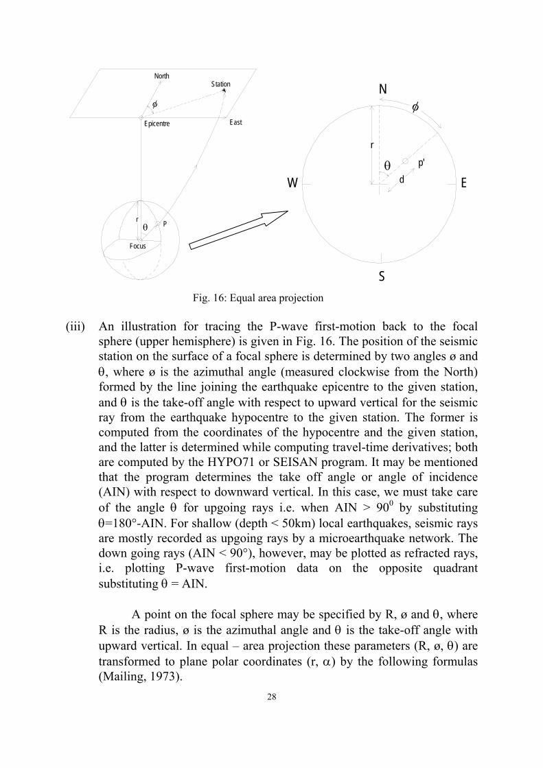
Fig. 16: Equal area projection

(iii) An illustration for tracing the P-wave first-motion back to the focal sphere (upper hemisphere) is given in Fig. 16. The position of the seismic station on the surface of a focal sphere is determined by two angles ø and θ, where ø is the azimuthal angle (measured clockwise from the North) formed by the line joining the earthquake epicentre to the given station, and θ is the take-off angle with respect to upward vertical for the seismic ray from the earthquake hypocentre to the given station. The former is computed from the coordinates of the hypocentre and the given station, and the latter is determined while computing travel-time derivatives; both are computed by the HYPO71 or SEISAN program. It may be mentioned that the program determines the take off angle or angle of incidence (AIN) with respect to downward vertical. In this case, we must take care of the angle θ for upgoing rays i.e. when AIN > 900 by substituting θ=180°-AIN. For shallow (depth < 50km) local earthquakes, seismic rays are mostly recorded as upgoing rays by a microearthquake network. The down going rays (AIN < 90°), however, may be plotted as refracted rays, i.e. plotting P-wave first-motion data on the opposite quadrant substituting θ = AIN.

A point on the focal sphere may be specified by R, ø and θ, where

R is the radius, ø is the azimuthal angle and θ is the take-off angle with upward vertical. In equal – area projection these parameters (R, ø, θ) are transformed to plane polar coordinates (r, α) by the following formulas (Mailing, 1973).

28

r = 2R sin (θ/2), α= θ

Since the radius of the focal sphere R is immaterial and maximum value of r is more conveniently taken as unity, the above eq. is modified to read

θθ=⎟

⎠⎞

⎜⎝⎛= ar ,

2sin2

This type of equal-area projection was introduced by Honda and Emura (1958) in fault-plane solution.

M

XS

W

θ = 33° SE= 14°

P

1C

N

2C

B

YN

θφ = 38°

= 58° NW

T

E

Fig. 17: P-wave first-motion plot and fault plane solution (Kayal, 1984)

(iv) Figure 17 illustrates a P-wave first-motion plot (upper hemisphere) for a

microearthquake recorded by a 20-station network in New Zealand (Kayal, 1984). Fifteen reliable first-motion data are used for the solution. Solid circles are used for compression and open circles for dilatation. The P-wave first-motions on the focal sphere are separated so that the adjacent quadrants have opposite polarities. These quadrants are delineated by two orthogonal great circles, the nodal planes. To do this, rotate the plot such that a great-circle arc on the net separates the compressions from dilatations as much as possible. In this example (Fig. 17), the arc MBN represents the projection of a nodal plane, which strikes 38° and dips 58° NW. It may be noted that the concave side of the plane points the dip direction in the upper hemisphere plot. So, it is important to mention about the use of the hemisphere. The pole or normal axis to this plane is the point C1 which is 90° from the great circle arc MBN. Since the second nodal plane is orthogonal to the first, its great circle-arc must pass through the point C1. To find the second plane, rotate the plot so that another great circle-arc passes through the point C1 and also separates the

29

compressions from dilatations. This arc XBY strikes 14° and dips 32° ESE as measured from the equal-area net. The pole or normal axis of the second plane is the point C2, and it lies on the first nodal plane.

(v) The intersection of the two nodal planes is represented by the point B

which is the position of the intermediate stress (σ2) axis or null axis. The plane normal to the null axis is represented by the great circle-arc C1P C2T which contains two important axes : the P-axis (σ1) and the T-axis (σ3). The P axis is 45° from C1 and C2, and in the dilatational quadrant, and the T axis is 90° from the P axis and lies in the compressional quadrant. The P-axis represents the direction of compressional stress, and the T-axis the direction of tensional stress. In fault-plane solutions the stress axes are more popularly expressed as the P, T and B, rather than σ1, σ3, and σ2 respectively. Now, if we select the first nodal plane MBN as the fault plane then the point C2 represents the slip vector. It may be mentioned that we cannot distinguish which nodal plane is the fault plane from the P-wave first-motion plot alone. The geological information of existing faults, the P-wave radiation pattern i.e. nodal character, distribution of the epicentres and the hypocentre-sections or depth-section of the earthquakes are used to infer the fault-plane. .

(vi) We can summarize our results from the above P-wave first-motion plot

as follows: (a) Nodal Plane-1 (preferred Fault Plane) :

Strike : 380, dip: 580 NW, slip angle : 550

(b) Nodal Plane-2 (Auxiliary Plane) : Strike : 140, dip: 320 ESE , slip angle : 320

(c) P-axis : strike : 3440, plunge: 740

(d) T-axis : strike : 1180, plunge: 120

(e) B-axis : strike : 2110, plunge: 110

(vii) The fault-plane solution (Fig.17) represents almost a pure normal faulting

(i.e. λ ~ 850 ) with a small left-lateral strike - slip motion as shown by arrows.

30

Earthquake Mechanism and Plate Tectonics Earthquake mechanism plays a major role in development of our understanding of global plate tectonics; their distribution is needed to map plate boundaries. The slip vectors of the earthquakes provide information about the direction of plate motion at individual boundary. The plate boundaries are divided into three types : (i) Spreading centre, (ii) Subduction zones and (iii) Transform fault. Oceanic Spreading Centre Focal Mechanism

Earthquake mechanisms from spreading centre are illustrated in Fig. 18. The spreading centre shows a portion of spreading ridge is offset by transform faults. New lithosphere forms at the ridges, then moves away. The relative motion of lithosphere on either side of a transform is in opposing directions. The direction of transform offset determines whether there is right-lateral or left-lateral motion.

Fig. 18: Source mechanisms of earthquakes at spreading centre.

The Fig. 18 shows the spreading centre is composed of north-south trending ridge segments, offset by transform faults, which trend approximately east-west. Both the ridge crest and transform faults are seismically active. The mechanisms show that the relative motion along the transform is right-lateral. The earthquakes occur exclusively on the active transform fault segment rather than on the inactive extension, known as fracture zone. No relative plate 31

motion occurs on the fracture zone, it is often marked by distinct topographic features due to contrast in lithospheric ages across it. The seismicity is different on the spreading ridges; normal faulting earthquakes are observed on the ridge crest; the modal planes trending along the ridge axis (Fig. 18). Subduction Zone Focal Mechanisms

ajority of large earthquakes occur in subduction zones; their focal mecha

Mnisms reflect various aspect of subduction tectonics. The Fig.19

illustrates some of the features observed in the Indo-Burma subduction zone.

hrust faulting are observed for the shallow earthquakes at the interface between overriding plate and subducting plate. Slip vector of the focal

Fig. 19: Source mechanisms of earthquakes at the subduction zone, Indo-Burma ranges (Rao & Kalpana, 2005)

T

mechanism may give the direction of plate motions. The flexural bending of the subducting plate, on the other hand, produces normal faulting earthquakes at shallower depth of 20~25 km, and thrust faulting earthquakes in the lower part 40-50 km. The observations constrain the position of neutral surface separating the upper extensional zone from the lower flexural zone, thus provide information on the mechanical state of the lithosphere. There has been some controversy whether, the normal faulting earthquakes as “bending” events or “slab pull” events. The deeper earthquakes in the Wadati-Benioff zone go down to 700 km, and their mechanism provide information about physics of the subduction process. The essence of the process is the penetration and slow

32

heating of a cold lithosphere in the warmer mantle. The thermal structure, seismic velocity, attenuation characters are diagnostic for the subducting plate.

Diffuse Plate - Boundary Focal Mechanisms

The continental crust is much thicker, less dense and has different

mechanical properties from oceanic crust. The plate boundaries in continents are often diffuse, and a broad zone of deformation is evident, such as India-Eurasian collision zone in the Himalaya or the Pacific-North America boundary zone in the western United States.

Fig. 20: Source mechanisms of earthquakes at the Himalayan collision zone.

In the Himalayan collision zone the earthquakes are characterized by

thrust mechanism and the plate boundary zone is wide (Fig 20). The Pacific-North American plate boundary, on the other hand, is extensional, essentially transform along the San Andreas fault system, and convergent in the eastern Aleutians. These changes are well reflected in focal mechanisms.

33

PAKISTAN

Fig. 21 : Source mechanisms of intraplate earthquakes, peninsular India (Kayal, 2000). Intraplate Focal Mechanisms

The intraplate earthquake mechanisms have important use to learn poorly understood tectonic processes of internal deformation of major plates. The seismicity of such regions is generally thought to be due to reactivation of pre-existing faults or weak zones in response to intraplate stresses. Intracontinental earthquakes occur less frequently than plate boundary event, recurrence estimates average 500-1000 yrs. As a result, understanding how these intraplate seismic zones operate is a major challenge. Source mechanisms of strong earthquakes occurred in peninsular India intraplate region are shown in Fig. 21.

34

ANNEXURE - 1

Modified Mercalli (MM) Intensity Scale (1956 version) (after Richter, 1958)

Intensity Description

I. Not felt. Marginal and long-period effects of large earthquakes.

II. Felt by persons at rest, on upper floors, or favourably placed.

III. Felt indoors. Hanging objects swing. Vibration like passing of light trucks. Duration estimated. May not be recognized as an earthquake.

IV. Hanging objects swing. Vibration like passing of heavy trucks; or sensation of a jolt like a heavy ball striking the walls. Standing cars rock. Windows, dishes, doors rattle. Glasses clink. Crockery clashes. In the upper range of IV, wooden walls and frame creak.

V. Felt outdoors; direction estimated. Sleepers wakened. Liquids disturbed, some spilled. Small unstable objects displaced or upset. Doors swing, close, open. Shutters, pictures move. Pendulum clocks stop, start, change rate.

VI. Felt by all. Many frightened and run outdoors. Persons walk unsteadily. Windows, dishes, glassware broken. Knickknacks, books, etc. off shelves. Pictures off walls. Furniture moved or overturned. Weak plaster and masonry D cracked. Small bells ring (church, school). Trees, bushes shaken visibly, or heard to rustle.

VII. Difficult to stand. Noticed by drivers. Hanging objects quiver. Furniture broken. Damage to masonry D, including cracks. Weak chimneys broken at roof line. Fall of plaster, loose bricks, stones, tiles, cornices also unbraced parapets and architectural ornaments. Some cracks in masonry C. Waves on ponds, water turbid with mud. Small slides and caving in along sand or gravel banks. Large bells ring. Concrete irrigation ditches damaged.

VIII. Steering of cars affected. Damaged to masonry C; partial collapse. Some damage to masonry B; none to masonry A. Fall of stucco and some masonry walls. Twisting, fall of chimneys, factory stacks, monuments, towers, elevated tanks. Frame houses moved on foundations if not bolted down; loose panel walls thrown out. Decayed piling broken off. Branches broken from trees. Changes in flow or temperature of springs and wells. Cracks in wet ground and on steep slopes.

IX. General panic. Masonry D destroyed; masonry C heavily damaged, sometimes with complete collapse; masonry B seriously damaged. General damage to foundations. Frame structures, if not bolted, shifted off foundations. Frames racked. Serious damage to reservoirs. Underground pipes broken. Conspicuous cracks in ground. In alluviated areas sand and mud ejected, earthquake fountains, sand craters.

35

X. Most masonry and frame structures destroyed with their foundations. Some well-built wooden structures and bridges destroyed. Serious damage to dams, dikes, embankments. Large landslides. Water thrown on banks of canals, rivers, lakes, etc. Sand and mud shifted horizontally on beaches and flat land. Rails bent slightly.

XI. Rails bent greatly. Underground pipelines completely out of service.

XII. Damage nearly total. Large rock masses displaced. Lines of sight and level distorted. Objects thrown into the air.

Masonry A, B, C, D. To avoid ambiguity of language, the quality of masonry, brick or otherwise, is specified by the following lettering.

Masonry A. Good workmanship, mortar, and design; reinforced, especially laterally, and bound together by using steel, concrete, etc.; designed to resist lateral forces.

Masonry B. Good workmanship and mortar, reinforced, but not designed in detail to resist lateral forces.

Masonry C. Ordinary workmanship and mortar; no extreme weaknesses like failing to tie in at corners, but neither reinforced nor designed against horizontal forces.

Masonry D. Weak materials, such as adobe; poor mortar; low standards of workmanship; weak horizontally.

36

37

References : Aki, K. 1965. Maximum-likelihood estimate of b in the formula 108 N = a – bM and its confidence limits, Bull. Earthquake Res. Inst., Tokyo Univ., 43: 237-239. Aki, K. 1966. Earthquake generating stress in Japan for the years 1961 to 1963 obtained by smoothing the first motion radiation patterns. Bull. Earthquake Res. Inst., 44: 447-471. Anderson, E.M. 1951. The dynamics of faulting and dyke formation with applications to Britain, 2nd ed. London. Crosson, R.S. 1972. Small earthquakes, structure and tectonics of the Puget Sound Region. Bull. Seis. Soc. Am., 62: 1171. Grassberger, P. and Procaccia, I. 1983. Characterisation of strange attractors, Phys. Rev.Lett. 50, 346-349. Guo, Z. and Ogata, Y. 1995. Correlation between characteristic parameters of aftershock distribution in time, space and magnitude, Geophys. Res. Lett., 22: 993-996. Guo, Z. and Ogata, Y. 1997. Statistical relations between the parameters of aftershocks in time, space and magnitude, J. Geophys. Res. 102:2857-2873. Gutenberg, B. and Richter, C.F. 1944. frequency of earthquakes in California, Bull. Seism. Soc. Am. 34 ; 185-188. Gutenberg, B. 1945 a. Amplitudes of surface waves and magnitudes of shallow earthquakes, Bull. Seism. Soc. Am., 35:3-12. Gutenberg, B. 1945 b. Amplitudes of P, PP and S and magnitudes of shallow earthquakes, Bull. Seism. Soc. Am., 35:57-69. Gutenberg, B. and Richter, C.F. 1954. Seismicity of the Earth and Associated Phenomena, Princeton University Press, New Jersey, 310 pp. Gutenberg, B. and Richter, C.F. 1956. Seismicity of the earth and associated phenomena, 2nd Edition, Princeton Univ. Press, P.310.

38

Hanks, T.C. and Kanamori, H. 1979. A moment magnitude scale, J. Geophys. Res., 84 : 2348-2350. Hirata, T. 1989. A correlation between the b-value and the fractal dimension of earthquakes, J. Geophys. Res. 94:7507-7514. Honda, H. and Emura, K. 1958. Some charts for studying the mechanism of earthquakes SCI Rep. Tohoku Univ., 5th ser. Geophys. 9, 113-115. Honda, H. 1962. Earthquake mechanism and seismic waves. J. Phys. Earth, 10:1-97. Kagan, Y.Y. and Knopoff, L. 1980. Spatial distribution of earthquakes : The two point correlation function, Geophys. J.R. Astron. Soc., 62: 303-320. Kayal, J.R. 1984. Microseismicity and tectonics at the Indian Pacific Plate Boundary : Southeast Wellington Province, New Zealand, Geophys. J.R. Astr. Soc. 77: 567-592. Kisslinger, C. and Jones, L.M., 1991. Properties of aftershocks in southern California, J. Geophys. Res., 96: 11947-11958. Lay, Thorne and Wallace, Terry, C. 1995. Modern Global Seismology, Academic Press, New York, USA, 521 p. Lee, W.H.K., Bennett, R.E. and Meagher, K.L.1972. A method of estimating magnitude of local earthquakes from signal duration, open file report, U.S. Geol. Surv. Main, I.G. 1991. Damage mechanism with long range interactions : correlation between the seismic b-value and the fractal two point correlation dimension. Geophys.J.Int., 107, 531-541. Mandelbort, B.B. 1982. The fractal Geometry of nature, W.H. Freeman, New York, 109-115. Mogi, K. 1962. On the time distribution of aftershocks accompanying the recent major earthquakes in and near Japan. Bull. Earthquake Res. Inst. 40: 107-124. Mogi, K., 1967. Earthquakes and fractures, Tectonophysics, 5, 35-55.

39

Nanjo, K., Nagahama, H. and Satmura, M. 1998. Roles of aftershock decay and the fractal structure of active fault systems, Tectonophysics, 287: 173-186. Ogata, Y. (1988) Statistical models for earthquake occurrences and residual analysis for point processes, Journal of American Statistical Association, Application, Vol. 83, No. 401, pp. 9-27. Omori, F. 1894. On aftershocks (in Japanese). Rep. Imp. Earthquake Invest Comm. 2: 103-139. Ouchi, T. and Uekawa, T. 1986. Statistical analysis of the spatial distribution of earthquakes – variation of the spatial distribution of earthquakes before and after large earthquakles. Phys. Earth planet. Inter., 44, 211-225. Pacheco, J.F., Scholz, C.H. and Sykes, L.R., 1992. Changes in frequency-size relationship from small to large earthquakes, Nature, 355: 71-73. Reid, H.F. 1910. The California earthquake of April 18, 1906, vol. 2 : The mechanics of the earthquakes, Carnegie Inst., Washington, D.C. Richter, C.F. 1935. An instrumental earthquake magnitude scale. Bull. Seism. Soc. Am., 25 : 1-32. Richter, C.F. 1958. Elementary seismology, W.H. Freeman and Co. San Francisco, USA. Scholtz, C. H. 1968. The frequency magnitude relation of microfacturing in rock and its relation to earthquakes, Bull. Seism. Soc. Am., 58, 39-415. Scholz, C.H. 1990. The mechanics of earthquakes and faulting, Cambridge Univ. Press, Cambridge. Shimazaki, T. and Nagahama, H., 1995. Do earthquakes occur at random, collectivities and individualities of earthquakes (in Japanese), Kagaku (Science), Tokyo, 65 : 241-256. Stauder, W. 1962. The focal mechanism of earthquakes, Adv. Geophys. 9, 1-76. Tinti, S., T. Vittori and F. Mulargia 1987. On the macroseismic magnitudes of the largest Italian earthquakes, Tectonophysics, 138, 159-178.

40

Toppozada, T. R. 1975. Earthquake magnitude as a function of intensity data in California and Western Nevada, Bull. Seism. Soc. Am., 65, 1,223-1,238. Tosi, P. 1998. serismogenic structure behaviour revealed by spatial clustering of seismicity in the Umbria-Marche region, (Central Italy), Ann. De Geofisica, 41(2) : 215-224. Utsu, T. 1961. A statistical study on the occurrence of aftershocks, Geophys. Mag., 30, 521-605. Utsu, T. 1969. Aftershocks and earthquake statistics, 1. Some parameters which characteristics an aftershock sequence and their interrelations. J. Fac. Sci. Hokkaido Univ., Geophys. 3 : 129- Xu, Y. 1992. A study on characteristics of the Information Dimension Di of the temporal and spatial distribution of earthquakes in an active fault zone. Acta seismological Sinica, 5(2), 389-398.