Forum on Income Mobility

347

National Tax JournalVol. LXIl, No. 2June 2009

Abstract - Inferences about earnings volatility across groups and time depend on the underlying models of earnings dynamics, data sources, earnings concepts, and sampling strategies. In this paper we evaluate a model of earnings dynamics in which the permanence of shocks varies by age and education. This specifi cation is consistent with observed earnings changes in administrative panel data, and also with the variance of earnings levels in multiple cross–section (synthetic panel) data. However, expanding the earnings concept to include self–employment and changing sampling strategy to include observations with minimal labor force attachment has fi rst–order effects, and may help explain why some studies conclude that earn-ings volatility is rising.

INTRODUCTION

Earnings volatility is of fundamental interest to many different groups of economists. Researchers studying

tax policy are interested in earnings volatility because of the implications for distributional analysis of tax burdens: in a progressive tax system, the more individual incomes vary over time, the more divergent are conclusions about effective tax rates when comparing annual and multi–year measures.1 Earnings volatility plays a crucial role in macroeconomics because of the impact that earnings uncertainty has on con-sumption behavior.2 Recently, earnings volatility has become an interesting policy question in its own right because a growing literature has argued that economic well–being has been adversely affected in recent decades because individual earnings became more volatile.3 The conclusion that earnings volatility increased is far from universal, however, as other John Sabelhaus

University of MarylandCollege Park, Maryland 20742

Jae SongU.S. Social Security AdministrationWashington, D.C. 20003

Earnings Volatility Across Groups and Time

1 See, for example, U.S. Congressional Budget Offi ce (2005) and Cilke, et, al. (2001). Related tax–oriented research has focused on “mobility,” meaning systematic movement of individuals across earnings groups over time–e.g., Auten and Gee (2007) or Kopczuk, Saez, and Song (2007). Mobility in that context is closely related to the “permanence” of earnings shocks as described in this paper.

2 Indeed, much of the basic research that led to the earnings decomposition in this and other papers was undertaken for the purpose of analyzing sto-chastic consumption models. See in particular Carroll (1992) and Deaton and Paxson (1994).

3 The best known of these is a series of papers by Moffi tt and Gottschalk in which they implement formal variance decompositions for earnings shocks. The most recent in this series is Moffi tt and Gottschalk (2008), and their other seminal contributions were Gottschalk and Moffi tt (1994) and Moffi tt and Gottschalk (2002). Dynan, Elmendorf, and Sichel (2007) analyze the same data using a less formal approach and come to basically the same conclusions.

NATIONAL TAX JOURNAL

348

studies have found that variability in earnings growth was fl at or even declin-ing since 1980.4

Inferences about earnings volatility across groups and time depend on the underlying models of earnings dynamics, data sources, earnings concepts, and sam-pling strategies. The analysis in this paper suggests that all of these inputs have likely played some role in the divergence of conclusions in previous studies. Our base–case model of earnings dynamics with stable permanent shocks that vary by age and education is consistent with a transi-tory component that has declined over time. However, altering the earnings con-cept to include self–employment income and changing the sampling strategy to include observations with minimal labor force attachment has fi rst–order effects on the results. Indeed, those effects may be enough to explain why some studies conclude that earnings volatility is rising.

Three data sets are used in this paper. The first is a one percent longitudinal sample of earners ages 25–55 between 1980–2006 drawn at random from the Social Security Master Earnings File (MEF). The advantage of longitudinal data is that one can measure and analyze changes in log earnings over various time periods, which is the key to our fi rst approach to modeling earnings volatility. The second is another longitudinal sample from the MEF, but this time for the 1940–1960 birth cohorts and linked to Survey of Income and Program Participation (SIPP) data fi les from the 1990s. For the purposes of this paper, the advantage of the SIPP data is that we know educational attain-ment, so we can investigate differences in earnings shocks by level of schooling. The third data set is a series of cross sections from the March Current Population Sur-vey (CPS) between 1970–2007. Although one cannot measure changes in earnings using the CPS cross–sections, the data are

useful for analyzing the variance of earn-ings levels over time in a synthetic panel framework, and the addition of labor force attachment variables makes it possible to investigate how sampling may be affect-ing the results.

The starting point for the analysis in this paper is the observation that the variance of earnings growth rates in the MEF longitudinal earnings data declined signifi cantly over the period between the early to mid 1980s and the early to mid 1990s, and has since remained fl at. How-ever, a decline in the variance of growth rates does not necessarily imply that vola-tility has fallen, because labor economists have long recognized the importance of distinguishing permanent and transitory earnings shocks. Permanent shocks refl ect differential earnings growth within some reference group that is expected to per-sist—another way to describe economic mobility. Transitory shocks are temporary (though not necessarily gone after one period) and thus associated with volatil-ity per se.

There are a few different ways to use panel data to separate earnings growth variability into permanent and transitory components. We use an approach sug-gested by Meghir and Pistaferri (2004) for measuring the variance of permanent shocks that is both intuitive and robust to alternative specifi cations of the time series properties of transitory shocks. Using that approach, our longitudinal earnings data suggest that (1) the variance of permanent shocks declines with age, (2) the variance of permanent shocks is higher for the col-lege educated, and (3) the variance of per-manent shocks has been constant (within age and education groups) over time.

If the variance of permanent shocks within groups has been relatively stable, and overall growth rate variability within groups is falling, that suggests the vari-ance of transitory shocks (volatility) must

4 U.S. Congressional Budget Offi ce (2008) and Sabelhaus and Song (2008).

Forum on Income Mobility

349

have fallen. Indeed, that fi nding would be consistent with evidence from the litera-ture on the “Great Moderation” in macro-economics (Davis and Kahn, 2008). Also, there was a signifi cant secular decline in U.S. unemployment rates (at least through our sample period), and unemployment is the event one would generally associ-ate with transitory shocks. However, the book is not completely closed on the decrease in transitory earnings shocks; Moffi tt and Gottschalk (2008) argue it is possible that transitory shocks actually got bigger but became more serially cor-related. Our residual approach—starting with total variation and subtracting per-manent shock variation—cannot distin-guish between changes in the transitory variance and changes (in the opposite direction) in the covariance of transitory shocks.

In addition to looking at the variability of earnings growth within groups and over time, one can characterize earnings dynamics by looking at the variance of earnings levels within an age group or birth cohort over time. The canonical model that underlies the transitory and permanent decomposition implies that the variance of earnings at any given age and point in time will depend on the vari-ance of transitory shocks at that point in time, the initial earnings dispersion for the age or cohort group in question, and the accumulated permanent shocks since that initial time period. If the stochastic earnings process is stable, one should see stable earnings variances in the synthetic cross section.

The synthetic cross section we develop is based on March CPS data. The advan-tage of this data relative to our administra-tive records is that we know self–reported labor force attachment, so we can inves-tigate how restricting the sample to those who worked full–time or eliminating de minimis earnings affects the answers. The

CPS data confi rms our inferences about a stable permanent shock variance (at least after 1980) while the overall variance of earnings (for our preferred measures) was falling, which is consistent with declining volatility. However, we also show that changing the sampling criteria to include observations with modest labor force attachment and very low self–employ-ment earnings has a dramatic fi rst–order effect on the estimated variances. The sampling criteria are very likely a part of the explanation why researchers have dis-agreed about trends in earnings volatility.

MEASURING THE VARIABILITY OF EARNINGS GROWTH RATES OVER TIME

Although the concept of earnings volatility may seem straightforward in principle, measuring it in practice requires a number of decisions about data, sam-pling, and choice of summary statistic. In this section, we use administrative panel data from Social Security earnings records to present some basic fi ndings about the standard deviation of one–period earn-ings growth rates over time. Although the estimated level of variability at any point in time depends on how the sample is chosen, all of the measures we present suggest a general decline in variability between the early 1980s and mid 1990s, and little change thereafter through the end of our sample in 2006.

There are two main longitudinal data sets used in this section and the two sec-tions that follow. Both data sets are ulti-mately based on Social Security earnings records in the Master Earnings File (MEF).5 The fi rst sample is a one percent random draw from the MEF, and the second is a draw from the MEF based on linkages to several panels of the Survey of Income and Program Participation (SIPP). The SIPP–linked data is useful because it introduces

5 The appendix has a complete description of the data sets used in this paper.

NATIONAL TAX JOURNAL

350

more demographic information than is available on the Social Security records. For our purposes, the SIPP provides the level of educational attainment used to further subdivide the sample when look-ing at various types of earnings shocks in subsequent sections. In both samples, data on wages from W2 reporting are used for all years back to 1980 and data on wages plus self–employment earnings are used for years after 1994.6

The decision about which age and/or cohort groups to include in the sample is somewhat dependent on the question being asked. The one percent random sample results presented here are generally based on ages 25–55—what we refer to as prime working years.7 In the SIPP, the main sam-ple is drawn for birth cohorts 1940–1960. The cohort restriction is set so the sample is mid–career around the points in time when the SIPP linkages are established (1990 through 1996), while generally assuring that the educational attainments are effec-tively completed for every observation (that is, the links are established for everyone 25 or older at the time of the survey).

The concept of earnings growth vari-ability used in this section is the standard deviation of the one–period change in log earnings. The standard deviation is a con-venient statistic, as the extent of variability is summarized in a single number, and the standard deviation is a useful starting point for distinguishing permanent from transitory earnings shocks. Focusing on the standard deviation also has its draw-backs, as it may hide important infor-mation about the symmetry of shocks, potentially allowing some very large per-centage changes to dominate the results even though their meaning is dubious.

In particular, a large percentage change in the standard deviation can mean large dollar changes near the average earnings, but it can also mean relatively small dollar changes at very low earnings. 8

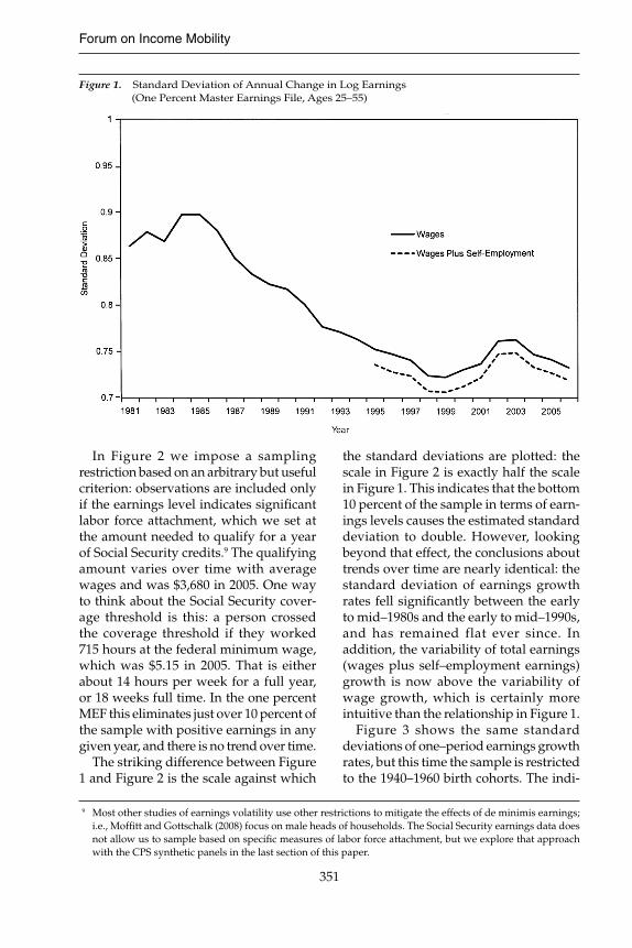
Figure 1 shows the standard deviation of one period changes in log earnings for the one percent MEF sample for 1981 through 2006. There is a signifi cant decline in earnings growth variability between the early to mid 1980s and the early to mid 1990s. However, there are two important observations about Figure 1 that under-score the need for an alternative sampling strategy in the remainder of the paper. First, the scale for the standard deviation is huge, ranging from about 90 log points in the early 1980s to just over 70 log points today. Simply interpreted, this means that something like one–third of the observa-tions have absolute earnings growth rates of 70 percent or more. The second obser-vation is that the growth rate of the sum of reported wages and self–employment earnings is actually less variable than wages alone, which is counter–intuitive.

Measuring the change in log earnings for any individual in two subsequent periods imposes a natural sampling restriction: their earnings have to be posi-tive in both years. However, that minimal sampling restriction means that observa-tions with very low earnings in any given year can have disproportionate effects on the estimated standard deviation. In par-ticular, a person whose earnings fall from $50,000 to $25,000 would make the same contribution to the standard deviation as one whose earnings fell from $1,000 to $500, because both are 50 percent declines. The signifi cance of the two declines is obviously very different.

6 Data on wages from W2s actually go back to 1978, but the sampling in the one percent fi le was not really rep-resentative until 1980. Before 1978, the wage and salary information is reported only up to the Social Security taxable maximum, which limits practical use for volatility studies. The self–employment data (taken from Form SE) was subject to top coding until the ceiling on taxation for Medicare was lifted in the early 1990s.

7 The conclusions do not change if we expand the sample to include everyone age 21–64. 8 Jensen and Shore (2008) focus on changes in the distribution of volatility over time, and fi nd that the overall

average increase in the PSID has been dominated by changes in variability for the most volatile households.

Forum on Income Mobility

351

In Figure 2 we impose a sampling restriction based on an arbitrary but useful criterion: observations are included only if the earnings level indicates signifi cant labor force attachment, which we set at the amount needed to qualify for a year of Social Security credits.9 The qualifying amount varies over time with average wages and was $3,680 in 2005. One way to think about the Social Security cover-age threshold is this: a person crossed the coverage threshold if they worked 715 hours at the federal minimum wage, which was $5.15 in 2005. That is either about 14 hours per week for a full year, or 18 weeks full time. In the one percent MEF this eliminates just over 10 percent of the sample with positive earnings in any given year, and there is no trend over time.

The striking difference between Figure 1 and Figure 2 is the scale against which

the standard deviations are plotted: the scale in Figure 2 is exactly half the scale in Figure 1. This indicates that the bottom 10 percent of the sample in terms of earn-ings levels causes the estimated standard deviation to double. However, looking beyond that effect, the conclusions about trends over time are nearly identical: the standard deviation of earnings growth rates fell signifi cantly between the early to mid–1980s and the early to mid–1990s, and has remained flat ever since. In addition, the variability of total earnings (wages plus self–employment earnings) growth is now above the variability of wage growth, which is certainly more intuitive than the relationship in Figure 1.

Figure 3 shows the same standard deviations of one–period earnings growth rates, but this time the sample is restricted to the 1940–1960 birth cohorts. The indi-

Figure 1. Standard Deviation of Annual Change in Log Earnings (One Percent Master Earnings File, Ages 25–55)

9 Most other studies of earnings volatility use other restrictions to mitigate the effects of de minimis earnings; i.e., Moffi tt and Gottschalk (2008) focus on male heads of households. The Social Security earnings data does not allow us to sample based on specifi c measures of labor force attachment, but we explore that approach with the CPS synthetic panels in the last section of this paper.

NATIONAL TAX JOURNAL

352

viduals in this restricted sample were somewhat younger than those in the one percent random draw (ages 25–55) in the beginning of the period, and somewhat older by the end. The oldest person (born in 1940) was only 40 at the beginning of the sample, and the youngest (born in

1960) was 45 at the end. Given the results to follow in subsequent sections, it is not surprising that the decline in earnings variability is larger for this group, because earnings growth variability is higher at younger ages. However, the basic conclu-sions from Figures 1 and 2 show clearly:

Figure 3. Standard Deviation of Annual Change in Log Earnings (Cohorts 1940–1960)

Figure 2. Standard Deviation of Annual Change in Log Earnings Above Social Security Threshold Only (One Percent Master Earnings File, Ages 25–55)

Forum on Income Mobility

353

restricting the sample to earnings above the Social Security threshold has a fi rst–order impact on the level of the standard deviation of earnings growth, but not on the pattern of changes over time. Figure 3 also shows that the SIPP–linked fi le has the same basic patterns as the one percent MEF for the 1940–1960 cohorts.

PERMANENT SHOCKS OVER THE LIFE CYCLE

The standard deviation of one–period earnings change presented in the last section is a good starting point for the analysis of earnings volatility. One key question that arises is whether any given unpredictable change in earnings growth (or “shock”) is permanent or transitory in nature. In this section we use a simple tech-nique suggested by Meghir and Pistaferri (2004) to show that the size of permanent shocks varies by age and education. In par-ticular, the standard deviation of perma-nent earnings shocks falls signifi cantly as people move from the beginning towards the middle of their working careers, and the variance of permanent shocks is much higher for the college educated than other groups at any given age.

The usual starting point for decompos-ing earnings shocks in labor economics is the canonical permanent and transitory earnings shock model,

yit = μit + εit

μit = μit–1 + ηit

where y is log earnings, μit is the slowly evolving permanent component that changes by ηit each period, and εit is the transitory component. In the simplest versions the transitory and permanent

shock terms (εit and ηit) are assumed to be uncorrelated with zero means and constant variances (σ 2

T and σ 2P).

In practical applications, the level of y is replaced by the gap between actual y and the predicted value of log earnings based on observable characteristics for each individual—the so–called “earnings differ-ential.” In this case, the two error terms are more appropriately described as exogenous zero–mean shocks because the explainable part of earnings growth by age, education, and other observables is removed. Thus, the canonical model basically explains how individuals’ earnings evolve over time rela-tive to their group average.

Even the simplest implementations of the canonical model also generally acknowl-edge an ARMA structure for εit. That is, shocks to earnings are not perfectly transi-tory or perfectly permanent—some shocks may have a large initial effect but then persist (with declining effects on earnings) for a few years, while others lead to perma-nent shifts in the earnings differential (at least until another permanent shock comes along). In general, the ARMA specifi cation makes estimation of the canonical model somewhat more complicated, because the distinction between transitory and perma-nent will depend on exactly how the ARMA is specifi ed and estimated, and in particular, which parameters are allowed to vary and along which dimensions.10

A recent paper by Meghir and Pistaferri (1994) offers a key insight into the nature of permanent versus transitory shocks that makes it possible to work around the ARMA specifi cation issue. This insight was also used extensively by Jensen and Shore (2008) in their analysis of growth rate variability in the Panel Survey of Income Dynamics (PSID), and what fol-lows builds directly on that analysis.11 The

10 See Moffi tt and Gottschalk (2008) for an excellent discussion of the problems inherent in distinguishing between permanent and transitory shocks. The analysis in that paper is the motivation for the approach taken here.

11 Although it is not the focus of the current paper, it is worth noting that a quick check of the distribution of the Meghir–Pistaferri moment in our data reveals the same skewness that Jensen and Shore (2008) fi nd in the PSID.

NATIONAL TAX JOURNAL

354

suggested Meghir–Pistaferri moment that identifi es permanent shocks under very general ARMA structures is given by,

Vt = Σi (yit – yit–2)·(yit+2 – yit–4)

The intuition underlying this estimator is straight–forward: high frequency (two year) changes in residual earnings growth rates that are correlated with low–enough frequency (six year) changes in residual earnings growth rates around the same period can be characterized as permanent shocks.

Figure 4 shows standard deviations of the Meghir–Pistaferri moment by age for the entire one percent MEF sample with earnings above the Social Security threshold. There are two sets of estimates for wages: the fi rst averages the estimated moments by age for the fi rst half of the sample (1984–1993), and the second

averages the estimated moments for the second half of the sample (1994–2004). The third line shows the average of the estimated moment by age for the sum of wages and self–employment earnings, which covers the period 1994–2004.

All three lines on Figure 4 indicate that the standard deviation of permanent shocks declines noticeably with age. This result is intuitive, because earnings distributions widen faster at younger ages as people are being sorted into their ultimate lifetime earnings groups (indeed, this principle is the basis for analyzing the variance of earnings lev-els in the last section of this paper). The results in Figure 4—both patterns and magnitudes of permanent shocks at each age—a are consistent with estimates of permanent shocks generated using a dif-ferent approach to error decomposition in Sabelhaus and Song (2008).12 Figure 4 also

12 The alternative approach, generally traced back to Carroll (1992), relies on the fact that earnings growth mea-sured at different frequencies will have different combinations of transitory and permanent shock components. Sabelhaus and Song (2008) use that logic to separate permanent and transitory shock variances across ages, education, and time. Their approach can be criticized because the ARMA structure is ignored in the estima-tion; the fact that those results and the results here based on Meghir and Pistaferri’s moment estimator are so close suggests that ignoring the ARMA structure is not a problem after all.

Figure 4. Meghir–Pistaferri Permanent Shock Standard Deviation by Age (Wages and/or Earnings Above Social Security Earnings Threshold)

Forum on Income Mobility

355

provides two other key pieces of infor-mation: the data suggest that permanent shocks to total earnings at any given age are slightly larger than permanent shocks to wages alone, and that there was little if any change to the levels of permanent shocks between the two halves of the sample period.

Figure 5 shows that the variance of per-manent shocks depends on educational attainment as well as age. This fi gure is constructed using the SIPP linked data with the wages–only data for the entire 1984–2004 period, so the cohort aging effect described in the last section is a possible confounding factor. However, the fact that the levels of permanent shocks at any given age do not seem to be varying across time (Figure 4) suggests that the overall levels of the Meghir–Pistaferri estimator (at any given age) should be comparable. Figure 5 bears this out, as the average for all education groups in the SIPP–linked data is nearly identical to the averages for the one percent sample (wages only) in Figure 4.

The key contribution of Figure 5 is that permanent shocks vary with both age and education. In particular, the variance of permanent shocks is larger for the college educated at any given age, which suggests more dispersion in their earnings (around the overall average earnings) at any given age. The differences in trajectories within the college–educated population are much larger than in other education groups, and this is refl ected in larger (permanent) differences in growth rates, especially at younger ages. The implication is that the variance of earnings levels in the college educated population will be rising faster at any given age, which cross–section data confi rms.

PERMANENT SHOCKS AND TRANSITORY RESIDUALS OVER TIME

In the canonical model each individ-ual’s idiosyncratic earnings differential is subject to permanent and transitory shocks in every period. Since the overall variability of earnings growth depends

Figure 5. Meghir–Pistaferri Permanent Shock Standard Deviation by Age (Wages Only, 1984–2004, Above Social Security Earnings Threshold)

NATIONAL TAX JOURNAL

356

on underlying permanent and transitory shocks, one is tempted to say that transi-tory shocks (volatility) must have declined in the United States since the early 1980s. This follows from the observations that overall growth rate variances fell (Sec-tion 2) while the variances of permanent shocks have remained stable (Section 3). However, subtracting the variance of per-manent shocks from the overall variance in each period leaves a combination of terms that involves transitory variances and covariances, which is best described as a transitory “residual.”

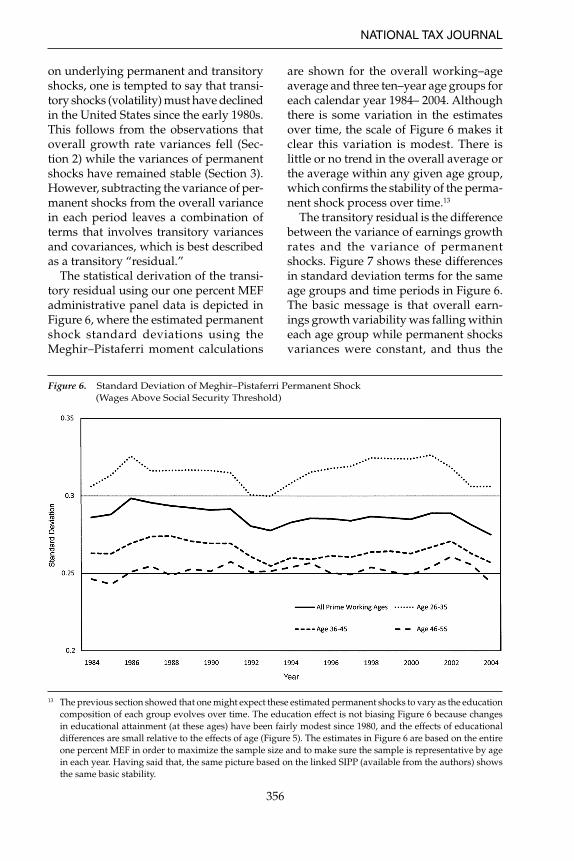
The statistical derivation of the transi-tory residual using our one percent MEF administrative panel data is depicted in Figure 6, where the estimated permanent shock standard deviations using the Meghir–Pistaferri moment calculations

are shown for the overall working–age average and three ten–year age groups for each calendar year 1984– 2004. Although there is some variation in the estimates over time, the scale of Figure 6 makes it clear this variation is modest. There is little or no trend in the overall average or the average within any given age group, which confi rms the stability of the perma-nent shock process over time.13

The transitory residual is the difference between the variance of earnings growth rates and the variance of permanent shocks. Figure 7 shows these differences in standard deviation terms for the same age groups and time periods in Figure 6. The basic message is that overall earn-ings growth variability was falling within each age group while permanent shocks variances were constant, and thus the

Figure 6. Standard Deviation of Meghir–Pistaferri Permanent Shock (Wages Above Social Security Threshold)

13 The previous section showed that one might expect these estimated permanent shocks to vary as the education composition of each group evolves over time. The education effect is not biasing Figure 6 because changes in educational attainment (at these ages) have been fairly modest since 1980, and the effects of educational differences are small relative to the effects of age (Figure 5). The estimates in Figure 6 are based on the entire one percent MEF in order to maximize the sample size and to make sure the sample is representative by age in each year. Having said that, the same picture based on the linked SIPP (available from the authors) shows the same basic stability.

Forum on Income Mobility

357

transitory residual was declining. The decline in residual variability was gradual and lasted through the late 1990s, before stabilizing or even slightly increasing around 2000, which is consistent with general observations about macroeco-nomic volatility.

The derived residual standard devia-tions in Figure 7 are not estimates of the standard deviation of transitory shocks. As Moffi tt and Gottschalk (2008) point out, the only thing we know from the canonical model is that the gap between overall earnings growth variability and permanent shock variances is a combina-tion of three terms,

Var(Δyit) – Var(ηit) = Var(εit) + Var(εit–1)

– 2·Cov(εit,εit–1)

Thus, one cannot say based on Figure 7 that the standard deviation of transitory shocks declined, because it is possible that changes in the covariance of transitory

shocks increased. However, this observa-tion about the transitory residual may simply underscore the fact that volatility itself is an imprecise concept. When do highly correlated transitory shocks cease to be part of volatility and become part of mobility?

THE VARIANCE OF EARNINGS BY AGE AND COHORT

The canonical earnings shock model also has testable implications for the vari-ance of earnings levels by age and cohort. For any given age group and at any point in time, the variance of earnings is the sum of the transitory variance, the initial (or age zero) permanent differential vari-ance, and the cumulated permanent shock variances. This characterization suggests a particular trajectory for the variance of earnings levels for any given cohort as they age.14 In this section we use synthetic panels from CPS cross sections between 1970–2007 to analyze earnings variances

Figure 7. Standard Deviation of Transitory Residual (Wages Above Social Security Threshold)

14 This is a key insight from Deaton and Paxson (1994).

NATIONAL TAX JOURNAL

358

across cohorts and time.15 The results are consistent with our fi ndings from looking at the variance of earnings growths using panel data, and the additional information in the CPS (especially labor force attach-ment) may be a clue as to why researchers have reached differing conclusions about trends in earnings volatility.

In the canonical earnings shock model the variance of log earnings for a given cohort at a point in time is the sum of three terms. Each cohort starts at the beginning of their working period (age zero) with an initial dispersion of log earnings dif-ferentials Var(μi0). In every year there are permanent shocks (ηit) that accumulate over time and transitory shocks (εit) that disappear after one year. If we check in on this cohort at some time t, the variance of log earnings differentials will be,

Var(yit) = Var(μi0) + ΣtVar(ηit) + Var(ε it)

Using this perspective, one can evaluate the stability of the stochastic earnings process by measuring log earnings vari-ance at a particular age over time, or by tracing log earnings variance for various birth cohorts by age.

Figure 8 shows variances of log wages for males age 30 to 39 over time computed a few different ways.16 The estimates which lead to the highest variances in every year are both based on the entire sample of people with positive earnings. The difference between the top two lines is that the highest variance in each year is for the log of wage levels, while the second highest is the log of the variance of wage differentials. The wage differential has the effect of age and education removed (it is

15 The March CPS data used in this paper was downloaded from the CPS–IPUMS site at the Minnesota Popula-tion Center (King, Ruggles, Alexander, Leicach, and Sobek (2004)).

16 We are motivated to focus on males 30 to 39 because this is the group Moffi tt and Gottschalk (2008) use to illustrate why they believe earnings volatility is rising. We fi nd—as they do—that the conclusions do not depend on exactly which age group is used to make the point.

Figure 8. Variance of Male Log Annual Wages (March Current Population Survey; Age 30–39)

Forum on Income Mobility

359

the residual after subtracting the mean). The gap between the top two lines rises over time because the earnings differences across education groups became more pronounced.

The two sets of estimates which lead to lower overall variances are both for earn-ings differentials, but these are based on restricted samples meant to eliminate the dominating infl uence of de minimis earn-ings. The solid line is based on a sample selected the same way as in our earnings growth calculations in the previous sec-tions: an observation is included only if earnings are above the Social Security qualifying threshold. The dashed line which lies close to the solid line is based on excluding observations that had earn-ings but self–reported that they were not full–time workers. As with our growth rate variance estimates based on the panel data, the effects of the sample restrictions are fi rst order.

From the perspective of the canonical earnings shock model, the key insight of Figure 8 is that all of the measures indicate that the variance of earnings

rose between 1970 and the early 1980s, but has since fallen or remained stable. The increase in log earnings variance throughout the 1970s is consistent with an increase in earnings growth variability, as fi rst reported by Gottschalk and Moffi tt (1994). The decline/stability after 1980 is consistent with the fi ndings presented in this paper.

One clue about why other researchers looking at recent data might be coming to different conclusions is shown in Figure 9. The only difference between Figure 8 and Figure 9 is the measure of earnings: Figure 8 is wages only, while Figure 9 includes wages and self–employment earnings. The scales of Figures 8 and 9 are the same, so the fi rst observation is that most of the variance measures—the exception is the Social Security threshold restricted con-cept—are noticeably higher. More impor-tantly, there is an increase after 1980 in the variance for the unrestricted samples and in the full–time only sample, which suggests that the combination of including self–employment and de minimis earn-ings is driving the results.

Figure 9. Variance of Male Log Annual Wages and Self–Employment Earnings (March Current Population Survey; Age 30–39)

NATIONAL TAX JOURNAL

360

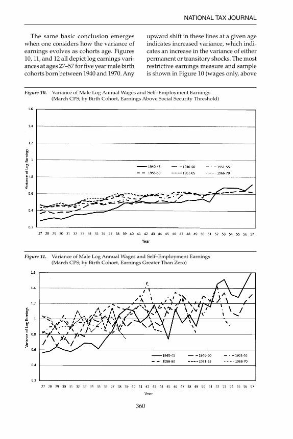
The same basic conclusion emerges when one considers how the variance of earnings evolves as cohorts age. Figures 10, 11, and 12 all depict log earnings vari-ances at ages 27–57 for fi ve year male birth cohorts born between 1940 and 1970. Any

upward shift in these lines at a given age indicates increased variance, which indi-cates an increase in the variance of either permanent or transitory shocks. The most restrictive earnings measure and sample is shown in Figure 10 (wages only, above

Figure 11. Variance of Male Log Annual Wages and Self–Employment Earnings (March CPS; by Birth Cohort, Earnings Greater Than Zero)

Figure 10. Variance of Male Log Annual Wages and Self–Employment Earnings (March CPS; by Birth Cohort, Earnings Above Social Security Threshold)

Forum on Income Mobility

361

Social Security threshold) and the most expansive measure and sample is shown in Figure 11 (wages plus self–employment earnings, greater than zero).

Focusing fi rst on Figure 10, and setting aside the oldest cohorts, one sees patterns that are generally consistent with the version of the canonical model presented in this paper. For example, the steeper slope at young ages indicates a larger variance for the permanent shocks. Also, the convergence of variances at any given age for the cohorts who reached working age after 1980 confi rms the stability in permanent shocks we found using the earnings growth data.

Figure 11 shows the same upward pat-tern in variances by age, but does not indicate the same sort of stability across cohorts, because the measure includes self–employment earnings and there are no threshold restrictions. However, there are also no systematic differences by cohort at any given age. The key message from Figure 11 is that expanding the earnings concept and setting the threshold at zero

just adds noise. Figure 12, which uses the same total earnings measure but restricts the sample to full–time only, is not much better. The upshot of both fi gures is that allowing de minimis earnings to enter vari-ance calculations has a fi rst–order effect on estimated variances, and it is easy to see how estimators based on sample variances could lead to spurious conclusions.

The sensitivity of estimated variance levels to de minimis earnings is strongly suggestive about the most promising directions for future research. First, focus-ing on just wages, it seems important to restrict the sampling to include only full–time earners in the earnings vari-ance estimates. This does not mean that exogenous events such as health–induced labor force withdrawal should be ignored, it just means they do not fi t into the logic of the simple canonical model. Second, it seems important to learn more about self–employed earnings—perhaps the decision to become self–employed says something about risk taking, and separate analysis of volatility is suggested.

Figure 12. Variance of Male Log Annual Wages and Self–Employment Earnings (March CPS; by Birth Cohort, Earnings Greater Than Zero, Full Time Only)

NATIONAL TAX JOURNAL

362

CONCLUSION

The canonical earnings shock model standard in microeconomic labor eco-nomics research has recently played an important role in the debate over whether earnings volatility in the United States is rising or falling. Different groups of researchers have started with the same basic framework and the same objective—decomposing earnings shocks into per-manent and transitory components—but reached very different conclusions about what is happening to earnings volatility. The results here suggest that the estimates are very sensitive to a combination of sam-pling restrictions and earnings measures. In particular, excluding observations with de minimis earnings—especially those with self–employment income—has a fi rst–order effect on sample variances and thus on inferences about earnings dynam-ics which rely on those variances.

The fact that inferences about earnings dynamics are highly sensitive to the inclu-sion of very low earnings suggests at least two possible directions for future research. The fi rst, suggested by Jensen and Shore (2008), is to move away from trying to characterize volatility for the whole population over time and to focus on how volatility varies across the population. The second direction involves separating out the sorts of shocks that affect realized earnings but do not fit nicely into the canonical model. In particular, the canoni-cal model does not explicitly incorporate the sorts of health or demographic shocks that might cause large swings in earn-ings. Some of those shocks are arguably a component of volatility, but in any event, isolating them will provide a clearer view of how the underlying permanent and transitory shocks that individuals face in the labor market have evolved over time.

Acknowledgment

The views of this paper do not represent those of the Investment Company Insti-tute or the Social Security Administration.

REFERENCES

Auten, Gerald E., and Geoffrey Gee. “Income Mobility in the U.S.: Evidence from

Income Tax Returns for 1987 and 1996.” Of-fi ce of Tax Analysis Paper 99. Washington, D.C.: U.S. Treasury Department, 2007.

Carroll, Christopher D. “The Buffer Stock Theory of Saving: Some

Macroeconomic Evidence,” Brookings Papers on Economic Activity 23 No. 2 (Fall, 1992): 61–135.

Cilke, James, Julie–Anne M. Cronin, Janet McCubbin, James R. Nunns, and Paul Smith. “Distributional Analysis: A Longer Term

Perspective.” Proceedings of the Ninety–Third Annual Conference on Taxation, 248–58. Wash-ington, D.C.: National Tax Association, 2001.

Davis, Steven J., and James A. Kahn. “Interpreting the Great Moderation: Chang-

es in the Volatility of Economic Activity at the Macro and Micro Levels.” NBER Work-ing Paper No. 14048. Cambridge, MA: Na-tional Bureau of Economic Research, 2008.

Deaton, Angus, and Christina Paxson. “Intertemporal Choice and Inequality.”

Journal of Political Economy 102 No. 3 (June, 1994): 437–67.

Dynan, Karen E., Douglas W. Elmendorf, and Daniel E. Sichel. “The Evolution of Household Income Vola-

tility.” Federal Reserve Board Finance and Economics Discussion Paper Series Work-ing Paper 2007–62. Washington, D.C., 2007.

Gottschalk, Peter, and Robert Moffi tt. “The Growth of Earnings Instability in the

U.S. Labor Market.” Brookings Papers on Eco-nomic Activity 25 No. 2 (Fall, 1994): 217–72.

**citation needed** Gottschalk, Peter, and Robert Moffi tt. 1992Jensen, Shane T., and Stephen H. Shore. “Changes in the Distribution of Income

Volatility.” University of Pennsylvania and The Johns Hopkins University. Unpublished manuscript, June, 2008.

King, Miriam, Steven Ruggles, Trent Alexander, Donna Leicach, and Matthew Sobek. Integrated Public Use Microdata Series,

Current Population Survey: Version 2.0.

Forum on Income Mobility

363

[Machine–readable database]. Minneapolis, MN: Minnesota Population Center [pro-ducer and distributor]. http://www.cps.ipums.org/cps (accessed **month, date, 2004).

Kopczuk, Wojciech, Emmanuel Saez, and Jae Song. “Uncovering the American Dream: Inequal-

ity and Mobility in Social Security Earnings Data Since 1937.” NBER Working Paper No. 13345. Cambridge, MA: National Bureau of Economic Research, August, 2007.

Meghir, Costas, and Luigi Pistaferri. “Income Variance Dynamics and Heteroge-

neity.” Econometrica 72 No. 1 (January, 2004): 1–32.

Moffi tt, Robert, and Peter Gottschalk. “Trends in the Transitory Variance of Male

Earnings.” John Hopkins University and Boston College. Unpublished manuscript, December, 2008.

Moffi tt, Robert A., and Peter Gottschalk. “Trends in the Transitory Variance of Earn-

ings in the United States.” The Economic Journal 112 No. 3 (March, 2002): 68–73.

Panis, C., R. Euller, C. Grant, M. Bradley, C.E. Peterson, R. Hirscher, and P. Stinberg. SSA Program Data User’s Manual. Baltimore,

MD: Social Security Administration, 2000.Sabelhaus, John, and Jae Song. “The Great Moderation in Micro Labor

Earnings.” University of Maryland and So-cial Security Administration. Unpublished manuscript, December, 2008.

U.S. Congressional Budget Offi ce. Effective Tax Rates: Comparing Annual and

Multiyear Measures. Washington, D.C., 2005. U.S. Congressional Budget Offi ce. Recent Trends in the Variability of Individual

Earnings and Family Income. Washington, D.C., 2008.

DATA APPENDIX

This paper uses two different longitudinal micro earnings data extracts from SSA’s master earnings fi le (MEF): SIPP matched extracts and SSA’s one percent detail earnings extract (Panis, et. al, 2000, Kopczuk, Saez, and Song, 2007). The

SSA’s MEF includes individuals’ annual Social Security covered earnings from 1951 to the pres-ent and annual wages directly taken from the W–2 starting from 1978. Other data elements included in the MEF are: the individual’s SSN, annual self–employment earnings, type of wage, deferred compensation contribution, and report year. Annual wages reported in the detail segment of the MEF are not top–coded, but earnings from self–employment (SE) are top coded until 1992. The Medicare taxable maximum was completely eliminated in 1993 and this rule change allowed SSA to keep SE earnings without top coding starting from 1993. To avoid the complication caused by the rule change, we exclude all SE earnings from our analysis.

Generally, SSA data are limited to informa-tion required for program administration and do not include individuals’ socio–economic characteristics, labor hours, and family struc-ture. Matched survey data combine the accu-racy of SSA administrative data with the variety of demographic and economic characteristics of individuals. SIPP matched samples used in this study are drawn from the 1990, 1991, 1992, 1993, and 1996 panels. The SIPP is a national survey conducted by the U.S. Census Bureau, designed as a continuous series of national panels since 1984, with sample sizes ranging from 14,000–36,700 interviewed households. The SIPP is a multistage, stratifi ed sample of the U.S. civilian, non–institutionalized popu-lation. Panel duration ranges from two and one–half to four years; each panel consists of six to twelve 4–month waves, depending on the panel duration. Each SIPP wave consists of both a core fi le and a topical module fi le. The core fi le contains the demographic, labor force, program participation, and income data designed to measure the economic situations of the individuals in the sample; these data are repeated at each interviewing wave.

The total number of observation interviewed in all core waves is 69,432, 44,373, 62,412, 62,721, and 95,398, respectively for 1990, 1991, 1992, 1993, and 1996 panels. Total number of observa-tions matched with Social Security detail earn-ings (wages only) data is 53,441, 32,977, 45,621,

NATIONAL TAX JOURNAL

364

44,602, and 75,903 for 1990, 1991, 1992, 1993, and 1996 panels respectively. For our analysis, we used samples born in 1940 through 1960 and those who earn above the amount required for four quarters of coverage (QC) each year. The amount needed to get one QC in 2000 was $780 (or $3,120 for 4QCs).

In order to get a better idea on how much of the standard deviation of logged earnings is

accountable for changes in education over the study period, we also repeat the same analysis controlling only for age and sex by using the one percent MEF extract. The one percent sample is selected on the basis of certain serial digits of the social security number and gener-ally considered to be random sample. Unlike the SIPP matched sample, the one percent sample includes institutionalized individuals.