Early Warning Models for Banking Supervision in Romania papers/Muntean Radu/muntean.radu... ·...

Academy of Economic Studies

Doctoral School of Finance and Banking

- Dissertation paper -

Early Warning Models for Banking Supervision in

Romania

MSc Student: Radu Muntean

Supervisor: Ph.D. Professor Moisă Altăr

Bucharest, July 2009

1

Table of contents

Abstract.........................................................................................................................2

1. Introduction..............................................................................................................3

2. Practice and literature review.................................................................................5

3. Methodology .............................................................................................................9

3.1. Binary dependent variable model....................................................................9

3.2. Ordered logistic model ...................................................................................10

3.3. Variable Selection ...........................................................................................11

3.4. Validation.........................................................................................................14

3.5. Predictions .......................................................................................................17

4. Data .........................................................................................................................18

5. Results .....................................................................................................................19

5.1. Rating downgrade ...........................................................................................19

5.2. Weak overall position .....................................................................................27

6. Conclusions .............................................................................................................38

Bibliography ...............................................................................................................40

Annex 1 – Variables and Signs .................................................................................43

Annex 2 – KS Test......................................................................................................46

Annex 3 – Monotony ..................................................................................................49

Annex 4 – Univariate Framework ............................................................................50

Annex 5 – Multicolinearity........................................................................................51

2

Abstract

In this paper we propose an early warning system for the Romanian banking sector, as

an addition to the standardized CAAMPL rating system used by the National Bank of

Romania for assessing the local credit institutions. We aim to find the determinants

for downgrades as well as for a bank to have a weak overall position, to estimate the

respective probabilities and to be able to perform rating predictions. Having this

purpose, we build two models with binary dependent variables and one ordered

logistic model that accounts for all possible future ratings. One result is that indicators

for current position, market share, profitability and assets quality determine rating

downgrades, whereas capital adequacy, liquidity and macroeconomic environment are

not represented in the model. Banks that will have a weak overall position in one year

can be predicted using also indicators for current position, market share, profitability

and assets quality, as well as, in this case, capital adequacy and macroeconomic

environment, the latter only for the binary dependent variable model, leaving liquidity

indicators out again. Based on the ordered logistic model’s capacity for rating

prediction, we estimated one year horizon scores and ratings for each bank and we

aggregated these results for predicting a measure of assessing the local banking sector

as a whole.

3

1. Introduction

Banking is one of the most intensively supervised industries world-wide due to the

high impact of bank failures on economic activity. Financial stability, a wide variety

of markets, infrastructure and even people’s personal comfort and safety depend on

the credit mechanism and the soundness of the banking sector. Therefore, all over the

world, governments grant authority to financial supervisory bodies and put them in

charge with the regulation, authorization and supervision of the financial institutions,

in order to limit the risks they undertake and the negative effect they might have on

other economic sectors.

Bank supervisors develop their knowledge about the banks running in their

jurisdictions by the means of on-site examinations and off-site surveillance. Although

useful in order to provide current and detailed data, the on-site examinations can be

costly for the supervisory authority by requiring the on-site teams to be sent at the

premises of the examined bank in order to have meetings, access files, check data

quality, analyze systems’ integrity and obtain results that can be used in assessing the

bank’s current situation. Moreover, on-site examinations can be burdensome to

bankers because of the human and logistical resources that they need to withdraw

from their current activities and make available to the on-site team demands.

Off-site surveillance aims at making the supervisor aware also of the bank’s situation

between on-site examinations. Financial data and other changes that occur at the

bank’s level are reported to the supervisory authority where are recorded and

analyzed. This way, the assessment of each bank is continuously updated and the

supervisors may decide whether and when another on-site examination is needed.

This dual approach might save resources for both, supervisor and supervised bank,

and might provide a clear picture of the risks undertaken by each bank as well as

inputs to assessing stability of the banking sector.

Some of the tools highly used in the off-site surveillance refer to the gathering of

relevant information within screens such as risk matrices and other specific tables that

assess each bank after a wide range of criteria. Historical experience and expert

opinion are some of the methods for selecting relevant criteria and their benchmarks.

Each bank is granted with an assessment as low-to-high, or a numerical rating for

each of the criteria employed. Then, all criteria-based ratings lead to the overall rating

of the bank.

4

Rating systems used by supervisory authorities provide valuable information about

the credit institutions analyzed within the same framework. Separating problematic of

well performing banks allow the supervisor to save resources by having the possibility

to focus more on the banks that are currently in distress. However, ratings carry

information about past situations and are more of an ex-post measure of the banks

status. Therefore, supervisors always need to consider expert opinion and recent

developments in order to have a better assessment of the credit institution.

Additionally, supervisors have come up with a class of tools that are able to predict

negative future events, thus gaining more time to act. Early warning (EW) models

have been used to predict negative events like bank failure, rating downgrade and

inadequate capitalization.

For the purpose of this paper we aim to find the determinants for rating downgrades

and the ones for a bank’s future overall position, in order to be able to estimate

probabilities for downgrades, bad ratings and also for each possible rating; these

results will then allow for rating prediction.

This paper is structured as follows: the next chapter is a brief introduction to current

practices and some of the literature relevant for the presented subject and chapter 3

presents the methodology highlighting the used models, the variable selection process

and model validation. Next chapter refers to data, as analyzed variables, periods and

discretions and is followed by Chapter 5 which presents the results focused on both

rating downgrade and weak overall position as main dependent variables. In this

chapter we show some of the intermediary results, the final models, validation,

prediction and other results. Chapter 6 highlights the most important results and

conclusions.

5

2. Practice and literature review

Supervisory authorities around the world have developed their own rating systems

aiming for a standardized approach to the different banks running business in their

jurisdictions as presented by BIS (2000). The CAMELS rating system was

implemented in 1980 in the United States of America by all three supervisory

authorities: Federal Reserve System (Fed), Office of the Comptroller of the Currency

(OCC) and Federal Deposit Insurance Corporation (FDIC). The rating system has six

components, referring to capital protection (C), asset quality (A), management

competence (M), earnings strength (E), liquidity risk (L) and market risk sensitivity

(S); to each of these components a grade from 1 (best) trough 5 (worst) is assigned.

CAMELS was followed by other rating systems like ORAP (Organization and

Reinforcement of Preventive Action) implemented by French Banking Commission in

1997, RATE (Risk Assessment, Tools of Supervision and Evaluation) implemented

by UK Financial Services Authority in 1998, RAST (Risk Analysis Support Tool)

implemented by Netherlands Bank in 1999, etc.

In the United States, the FDIC implemented the SCOR (Statistical CAMELS Off-site

Rating) model in 1995. SCOR is quarterly run based on data reported by credit

institutions and uses an ordered logit model of CAMELS ratings to estimate likely

downgrades of banks with a current composite CAMELS rating of 1 and 2. This is

explained by the higher attention already given by the supervisor to banks with on-site

examination rating of 3, 4 or 5. The model flags for review banks that are currently

strong or satisfactory but have a probable downgrade. The current rating is compared

to the one-year prior financial data and the coefficients found are employed to

estimate future ratings. The assumption is that the relation between current rating and

prior data will hold for future rating and present data.

SCOR uses a step-wise estimation in order to eliminate not statistically significant

variables. Many of the variables that are input to this model are also input to the

SEER (System for Estimating Examination Rating) model of the Federal Reserve,

although the prior CAMELS rating is included only in the SEER rating model.

The time horizon for rating estimation under SCOR is between four and six months.

Accuracy of the output has been shown to decrease beyond the six month period.

The output of this model is a table giving the probabilities that the next rating will be

each of the five possible ratings. A downgrade appears when a bank with a rating of 1

6

or 2 goes to a rating of 3,4 or 5. Also, the model provides a SCOR rating as the sum

of the possible ratings weighted with their probability. Areas of concern are

highlighted by comparing the bank with a “Median 2 Bank”, which is a typical bank

with a rating of 2.

Rating downgrade models share strong similarities with bankruptcy prediction

models. Beaver (1966) performed an early univariate discriminant analysis using 30

financial ratios for 158 firms, which found that cash-flows/equity and debt/equity can

be useful in default prediction.

Altman (1968) developed a scoring function, using multivariate discriminant analysis

(MDA), in order to discriminate between the two possible events. The variables used

together within the function were also specific for the purpose of bankruptcy

prediction.

The logistic regression was first used within a bankruptcy prediction framework by

Ohlson (1980). The variables are used in a multivariate framework as it is the case for

MDA but the scoring function is linear with regard to the log odd of default. Logit

models are preferable to MDA as the latter assumes that the covariance matrices are

the same for bankrupt and non bankrupt firms, it also assumes normally distributed

variables and, most important, are not able to provide a framework for performing

significance tests for the model parameters.

Over the last decades, the increasing interest of both supervisors and academics in

rating models and early warning systems has led to an economic literature able to

provide new methods and to raise new issues with respect to models used in bank

supervision.

As credit institutions are not usually defaulting often enough in order to provide for a

significant data base and therefore a significant statistical model, many papers refer to

inadequate capitalization, rating downgrades or other lesser negative events that are

also of high interest for assessing the stability of a bank.

In this respect, Jagtiani et al (2000) tested the efficacy of EW models as tools for the

prediction of capital inadequate banks using a sample of U.S. banks with capital

between $300 million and $1 billion. Logit and trait recognition analysis (TRA)

models were generated and compared trough a testing period. Findings showed the

importance of TRA in highlighting complex interaction variables useful in predicting

banks with deficient capital. Both the logit and the TRA models had a reasonable

7

degree of accuracy and they were considered a powerful tool for detecting one year in

advance inadequately capitalized banks.

Kolari et al (2000) used logit and TRA models to predict large U.S. bank failures. The

models were developed from an original sample and tested for predictive ability in the

holdout sample. Both models performed well, but TRA outperformed logit models in

overall accuracy, large bank failure accuracy, weighted efficiency scores. The paper

concluded that TRA models can identify variables interactions relevant for prediction

and therefore can provide valuable information about the future large bank failures.

Regarding rating downgrade, Gilbert et al (2000) compared such a model with a

currently employed banking failure prediction model (SEER) in use at the Federal

Reserve. Because of the small number of bank failures, the SEER coefficients are

mostly “frozen” and over time, the ability of the downgrade model in predicting

downgrades improves relative to that of the SEER model in predicting failures. This

paper concludes that a downgrade model may be useful in banking supervision and

shows the higher accuracy of a frequently re-estimated model.

Other studies like Gilbert et al (2002) argue that rating downgrade prediction models

may not clearly outperform failure prediction models, especially in tranquil periods.

However, it should be noted that there is a consensus over the fact that a rating

downgrade prediction model is an important informational supplement to supervisors

and even though it should not rule out expert opinion and other supervisory tools, it

should be used for highlighting possible problematic banks.

The models employed for rating systems can be validated through variety of

techniques. Engelmann et al (2003) analyzed useful tools for discriminatory power

such as the Cumulative Accuracy Profile (CAP) and the Receiver Operator

Characteristic (ROC). The summary statistics of CAP and ROC were proved to be

equivalent and the comparability of different models according to both statistics is

stated only for the same input data. For this reason, one could use Area Under ROC

(AUROC) alone in order to capture the discriminatory power of a model.

With respect to statistical issues concerning early warning models we refer to Hosmer

and Lemeshow (2000) who have thoroughly presented practical steps, problems and

discretions available when working with a logistic regression.

Studies performed on U.S. banks or cross-European banks samples have met with the

choice between different types of early warning system models. That is because on

8

such samples one could identify bank failures or inadequate capitalized banks and

therefore develop a model for predicting these events.

Banking sectors in most emerging countries have fewer banks and the data history is

shorter. Supervisors in these jurisdictions also employ tools based on current

assessment of banks but due to this issue they are usually not able to predict bank

failures or inadequate capitalization as early warning models, as these kind of

negative events have not happened enough to provide for a significant database.

However, implementation of rating downgrade prediction models is possible.

In Romania, in accordance with the Government Emergency Ordinance no. 99/2006,

the banking supervisory authority is granted to the National Bank of Romania (NBR).

Within the NBR there are several Departments directly connected to the banking

sector, with respect to regulation, authorization, financial stability and prudential

supervision. Changes in management, shareholders, financial situation of banks, as

well as current and past financial data and other relevant information are all actively

analyzed by the NBR, mainly within the Supervision Department (SD).

Commercial banks are assessed regarding the risks they undertake both by on-site

examinations and by off-site surveillance. The CAAMPL uniform rating system refers

to six components that are checked by the supervisor and rated in order to obtain a

final score and then an overall rating of the bank:

- capital adequacy (C);

- shareholders’ quality (A);

- assets’ quality (A);

- management (M);

- profitability (P) and

- liquidity (L).

Banks are rated from 1 (best) to 5 (worst) for each indicator included in each of the

six components and then the supervisor calculates aggregated ratings for the

components and an overall rating for the bank.

9

3. Methodology

3.1. Binary dependent variable model

In order to build an early warning model for the prediction of CAAMPL rating

downgrades we have employed a logit methodology. Then, the same methodology has

been applied for prediction of banks receiving a bad rating in one year horizon.

Firstly, we assume an unobservable dependent variable y* related to a binary

observed variable y, which represents a CAAMPL rating downgrade (y=1) versus a

constant or upgraded CAAMPL rating (y=0).

(1) ⎩⎨⎧

=>=

otherwiseyyify

i

ii

,00:,1 *

The latent variable y* is explained by the vector of bank’s financial ratios and other

individual figures as well as macroeconomic environment xi and the vector of

estimated coefficients β.

(2) iinniii

iii

xxxy

orxy

εββββ

εβ

+++++=

+=

...

:,

22110*

'*

The term εi is logistic distributed, thus having the logistic cumulative distribution

function:

(3) xe

xF −+=

11)(

The probability that a bank will have a downgraded rating can be expressed as

follows:

(4) β

ββ

βεβ

'

11)(),|1(

)()0(),|1( '*

i

i

xiii

iiii

exFxyP

xPyPxyP

−+≡==⇒

<−≡>==

The model’s coefficients are contained in the β vector and they need to be estimated.

The maximum likelihood method (MLE) assumes that each observation is extracted

from Bernoulli’s distribution. Therefore, a rating downgrade event has the attached

probability F(xi’β) making the probability of a non-downgraded rating event 1-

F(xi’β). The probability mass function is the product of the individual probabilities:

(5) ∏∏==

−×====0

'

1

'2211 ))(1()(),...,,(

ii yi

yinn xFxFyYyYyYP ββ

10

The likelihood function should be maximized with respect to the vector of

coefficients.

(6) [ ] [ ]NDN

i

DNN

ii xFxFL ))(1()()( '

1

' βββ −×=∏=

In order to obtain a more convenient expression to maximize we employ the

logarithm:

(7) { }∑=

−−+−−=N

iiiii xFyxFyL

1

'' ))(ln()1())(1ln()(ln βββ

The coefficients have been estimated using the quadratic hill climbing algorithm,

which, in order to achieve convergence, employs the matrix of secondary differentials

of the log likelihood function.

The estimated coefficients should be analyzed carefully noting that their size does not

necessarily carry significant economic information. However, the sign of each

coefficient is important as it shows how the dependent variable is influenced by a

variation in each variable. For instance, positive coefficients show that their

respective variables’ variations influence the downgrade probability in the same

direction as that of the variations which took place.

The marginal effect of the explanatory variables xj on the dependent variable is given

by βj weighted with a factor f depending on all the values in x.

(8) jiij

ii xfx

xyEββ

β)(

),|( '−=∂

∂, where

dxxdFxf )()( = is the density function

corresponding to F.

3.2. Ordered logistic model

Secondly, we considered an ordered logistic model. In this approach, the dependent

variable is assumed to represent ordered or ranked categories. The one year future

CAAMPL rating is mapped into the different values of y. The dependent variable in

an ordered logistic model is considering a latent variable, like in the case of the binary

dependent variable model previously presented.

(9) iii xy εβ += '*

The observed response yi is obtained from yi*, based on the following rule:

11

(10)

⎪⎪

⎩

⎪⎪

⎨

⎧

<

≤<

≤

=

−*

1

2*

1

1*

:,

:,2

:,1

i

i

i

yifM

yif

yif

y

M

i

γ

γγ

γ

The probabilities for the dependent variable to take each of the values allowed for are

given as follows:

(11)

⎪⎪

⎩

⎪⎪

⎨

⎧

−−==

−−−==

−==

− )(1),,|(

)()(),,|2(

)(),,|1(

'1

'1

'2

'1

βγγβ

βγβγγβ

βγγβ

iMii

iiii

iii

xFxMyP

xFxFxyP

xFxyP

, where F is the cumulative

distribution function of ε. For the purpose of this application, F was selected as being

the logistic cumulative distribution function.

The threshold values γ are important by determining the value of the dependent

variable, based on the score xi’β. In order to estimate the threshold vector γ, as well as

the β coefficients, the log likelihood function has to be maximized.

(12) ( )( ) ( )∑∑= =

=⋅==N

ii

M

jii jyxjyPL

1 1

1,,|ln)(ln γββ , where 1(x) is an indicator

function which takes the value 1 for a true argument and 0 for a false argument.

3.3. Variable Selection

While building a logit model, a key issue is the selection of explanatory variables. In

this regard, we considered to steps structured by Hosmer and Lemeshow (2000) for

the process of variable selection as well as other useful filters aimed to discriminate

between relevant and irrelevant explanatory variables.

For the first filter we considered the attribute of the explanatory variables to

discriminate between downgrades and non-downgrades. In this respect, we employed

a two-sample one-sided Kolmogorov-Smirnov test to determine whether the two

groups are drawn from the same underlying population, the null hypothesis of the K-S

test. We calculate the percentage of XND and XD less than each value x of the tested

variable and we record x for which the difference between the two figures is

maximum. The K-S statistic equals the maximum difference between XND and XD.

(13) [ ]DNDxXXKS −= max

The p-value of the test is p=e-2*λ^2 , where λ is given by:

12

(14) ⎟⎟⎟⎟

⎠

⎞

⎜⎜⎜⎜

⎝

⎛

×

⎟⎟⎟⎟

⎠

⎞

⎜⎜⎜⎜

⎝

⎛

+×

+++×

= 0,11.012.0max KS

DNDDNDDND

DNDλ , where ND is the number

of non-downgrades and D is the number of downgrades.

The main purpose of the K-S test filter is to eliminate variables that clearly do not

discriminate between downgrades and non-downgrades. However, this test is also

used in order to obtain the sign of the discrimination, explicitly whether the variable is

generally higher for future downgraded banks or lower. This result will be compared

to the following tests so that the sign of the explanatory variable with regard to the

dependent variable could be examined more carefully. The threshold for this test was

set at the 0.1 level of the p-value so that variables without a clear economic sense to

be eliminated, but was not set lower to avoid excluding potentially relevant variables.

As second filter, we analyzed the monotony assumed by a logit model. In this respect,

for each explanatory variable, we built a linear regression between the logarithm odd

against the mean values for several data subsets and checked if the assumptions made

for the relation between the dependent variable and explanatory variable are

respected.

(15) ii

i xRD

RD101

ln ββ +=⎟⎟⎠

⎞⎜⎜⎝

⎛−

, where RD is the historical rate of Downgrade and xi

is the average of the explanatory variable, both built on the data subsets.

The variables selected after these two filters are analyzed within a univariate logit

model framework. Hosmer and Lemeshow (2000) proposed a threshold of 0.25 for the

p-values of variables in univariate models. Variable selection can take into account p-

values, likelihood values, as well as AUROC calculated for each univariate model.

(16) ii

i xPD

PD101

ln ββ +=⎟⎟⎠

⎞⎜⎜⎝

⎛−

, where PD is the probability of Downgrade and xi is

the explanatory variable, both chosen over the entire estimation sample.

A fourth filter is given by colinearity tests. It should be noted that any correlation

between selected variables should make economic sense. Variables with a correlation

coefficient above a threshold are analyzed and the one which has a higher

performance in univariate models is selected.

13

Explanatory variables which have passed all the filters are subsequently analyzed in a

multivariate framework.

Backward selection method implies continuing with all the selected variables in a

multivariate model. Like structured in Hosmer and Lemeshow (2000), we examined

the Wald statistic for each variable and we compared the coefficient of each variable

with coefficients obtained in univariate models. It is important to see whether the

signs of the coefficients change or whether its size is highly volatile.

Variables that pass these tests are employed in a new multivariate model, for which

again the coefficients are examined. A new model is compared with the previous

larger model and in case the analyzed variable is considered not providing additional

information to the model, it will be rejected.

This process of eliminating, refitting and comparing continues until all the variables

included in the model are statistically significant as well as economically significant,

also checking whether other relevant variables remained outside the model.

In a forward selection method, after we decided which variables will be used in a

multivariate model, we introduced one variable at a time, in their univariate

performance order. If the new model is superior to the old model and if all the

estimates are significant, the variable is accepted and therefore other variable is

analyzed for selection in the new model.

Variable selection for predicting banks receiving a bad rating in one year horizon is

similar to the methodology presented for the prediction of rating downgrades.

In this case, a Kolmogorov – Smirnov test is applied to observe the discrimination of

each variable between the different one year future ratings. Analyzing variables in this

respect is more complex as it is required that they discriminate between banks in high

and low ratings, also having the option to check the downgrades discrimination.

Monotony must also be respected for each selected variable compared to the

logarithm odd of historical rate of each future rating.

A third test is based on the univariate models and checks the significance of each

parameter estimated in the univariate model built for each tested variable.

The colinearity filter is similar to the filter employed for rating downgrades

prediction, therefore the variables with a correlation above the threshold are analyzed

and the one with a lower performance in a univariate framework is rejected.

The variables selected after the four filters are used in order to build a multivariate

model. Both backward and forward selection methods are similar to the methods used

14

for the rating downgrades prediction, noting that the dependent variable is in the case

of binary dependent variable model the probability to receive a bad rating,

respectively the probability of each rating, in a one year horizon, for ordered logistic

model.

3.4. Validation

When the steps within the variable selection are completed, the remaining variables

enter the final model, which has to be validated in order to be considered proper for

the intended purpose and to be used for prediction.

While the models are useful in estimating probabilities of downgrades, it is necessary

to select a threshold above which the dependent variable will be estimated as 1,

meaning a rating downgrade. This threshold will be estimated based on the

minimization of a loss function which assesses the “loss” of the supervisory authority

using the model, depending on the Type I (downgrades occurred when non-

downgrades were estimated) and Type II (non-downgrades occurred when

downgrades where estimated) errors.

Estimated Equation

Dependent

variable = 0Dependent

variable = 1 Total estimated

Estimated dependent variable = 0

Correctly estimatednon-downgrades

Unexpecteddowngrades

(Type I Error)Estimated

non-downgrades

Estimated dependent variable = 1

Unexpected non-downgrades

(Type II Error)Correctly estimated

downgradesEstimated

downgrades

Total Non-downgrades Downgrades Total Sample

Therefore, the loss function of the supervisory authority has the following

specification:

(17) ( ) 2211 )()( ωεωεϕ ×+×= ccc , where ε(c) are Type I and Type II errors,

depending on the cutoff value c and ω are their respective weights.

These weights will be selected by the decision maker and the cutoff will have the

value of c when the loss function is minimized.

15

Another tool used for validation is the Receiver Operator Characteristic (ROC) Curve.

This method has the advantage of an easily understandable graphic representation as

an area part of the area of a square, which represents the performance of the perfect

model. In order to calculate the area under the ROC Curve (AUROC), we need the

following relations:

(18) ND

cHcHR )()( = , where HR(c) is the hit rate for cutoff c, H(c) is the number of

rating downgrades estimated correctly with cutoff c and ND is the total number of

rating downgrades. Hit rate is corresponding to the concept of sensitivity, as the

probability of detecting a true signal.

(19) NND

cFcFAR )()( = , where FAR(c) is the false alarm rate for cutoff c, F(c) is the

number of false alarms with cutoff c and NND is the total number of rating non-

downgrades. False alarm rate is corresponding to the concept of specificity, as

FAR=1-Specificity is the probability of detecting a false signal.

Having calculated the hit rate and the false alarm rate and plotting them together we

obtain the ROC Curve and the AUROC is subsequently calculated.

(20) )()(1

0

FARdFARHRAUROC ∫=

0

0.1

0.2

0.3

0.4

0.5

0.6

0.7

0.8

0.9

1

0 0.2 0.4 0.6 0.8 1

Probability cutoff

Sens

itivi

ty/S

peci

ficity

SpecificitySensitivity

ROC Curve

0

0.1

0.2

0.3

0.4

0.5

0.6

0.7

0.8

0.9

1

0 0.2 0.4 0.6 0.8 1

1-Specificity (FAR)

Sens

itivi

ty (H

R)

ROC Curve is obtained plotting HR and FAR over all possible probability cutoffs.

Area under ROC ranges from zero to one and provides a measure of how the model

discriminates between the realization of the dependent variable and the opposite

event.

As general rule for model performance, we use the following thresholds for AUROC:

16

If AUROC<0.5 Failed test – less than chance

If 0.5<=AUROC<0.6 Failed test

If 0.6<=AUROC<0.7 Poor test

If 0.7<=AUROC<0.8 Fair test

If 0.8<=AUROC<0.9 Good test

If 0.9<=AUROC Excellent test

While the AUROC indicates the discriminatory power of the model, this figure alone

may need to be analyzed with respect to the sample used in its calculation. Therefore,

we used a Bootstrap methodology, generating 1000 AUROC figures based on

different samples from a distribution identical to the empirical distribution of the

original sample.

This method allows us to assess the stability of the AUROC around the original

estimated value and to obtain variation intervals around this value.

In order to assess the goodness-of-fit of the model we used a Hosmer-Lemeshow test.

In this respect, we divided the sample in g groups and we compared the estimated

probability of downgrade with the empirical percentage of downgrades for each

group. The HL Test statistic for a model with correct specification follows a Chi-

square distribution with (g-2) degrees of freedom and is calculated as follows:

(21) ( )

( )∑= −

−=

g

k kkk

kkk

nno

C1

'

2'

1ˆ

πππ

, where nk’ is the total number of subjects in the kth group,

∑=

=k

jjk yo

1

, yj is the indicator of rating downgrade, kπ is the average estimated

probability for group k.

0.76 0.78 0.8 0.82 0.84 0.86 0.88 0.9 0.92 0.940

50

100

150

200

250

300

350

17

3.5. Predictions

Once the variables have been selected and the model has been validated, for both

binary dependent variable and ordered logistic models, the dependent variable is

calculated. In sample, this is done using the values of the ratios already used in

estimation, while out of time the dependent variable is calculated based on values of

the ratios not included in the estimation.

The estimated dependent variables are compared to the realized values in sample and,

particularly, out of time. While for the binary dependent variable model the dependent

variable is easily comparable with the percentage of rating downgrades/number of

banks receiving a bad rating, for the ordered logistic model the probabilities

calculated for each possible rating have to be manipulated in order to obtain values

comparable with an observable variable.

Firstly, the ordered logistic model can be used for the same purpose as the binary

dependent variable model, for instance, in calculating a probability of rating

downgrade.

(22) ∑−

=+=

1

1,

M

rjjii PPD , where M is the total number of ratings, r is the current rating

of the observed bank i and Pi,j is the probability that the observed bank i will have the

rating j in one year horizon.

Moreover, the probability of downgrade estimated with the ordered logistic model can

be compared to the one estimated with the binary dependent variable model and the

validation results can be analyzed as well. This can also be done in the case of

predicting bank receiving a bad rating.

The ordered logistic model can also provide for a shadow rating which is the average

of the possible ratings, weighted with their respective estimated probabilities.

(23) ∑=

×=M

jjjii RPSR

1,

Considering a naive model predicting the one year horizon rating to be the current

rating, the estimated shadow rating is expected to perform better. Both predictions are

comparable with the realized rating, observable in one year, using a distance function

as following:

(24) ( )2

1∑=

−=N

iii RRD , where iR is the estimated rating for observation i, N is the

number of analyzed observations and Ri is the observed respective rating.

18

4. Data

For the purpose of this paper, the input data contains both microeconomic and

macroeconomic variables (Annex 1) from December 2002 to December 2008.

Most of the microeconomic data is taken from the reports provided by a sample of

about 30 Romanian banks to the National Bank of Romania, their supervisory

authority. These financial ratios are structured on the following four main

components: assets quality, capital adequacy, profitability and liquidity. Other

variables with specific values for each bank and therefore considered to be

microeconomic are the CAAMPL rating and the bank’s position in the market, as both

assets and loans based market share.

The other part of the input data consists on several indicators at macroeconomic level

which have the same values for different banks at the same moment in time. These

variables are current values and last variations of indicators related to interest rates,

exchange rates, wage, industrial production, unemployment rate and inflation.

It should be noted that the financial ratios are also comparable because of the

reporting regulations and procedures maintained by the National Bank of Romania.

Moreover, the data only takes into account banks which are Romanian legal entities,

excepting the savings banks for housing. We have not selected branches of foreign

banks that are not Romanian legal entities because these banks have different

reporting regime and also a different overall status, due to the direct involvement of

the parent bank and home country supervisory authority.

The banks selected into analysis have a cumulative assets market share between

90.95% and 94.66% over the period making the results obtained for this sample

relevant for the entire Romanian banking sector.

The available data was divided into three samples. The first period from December

2002 to December 2006 containing 480 observations for financial ratios and

indicators is used to estimate the parameters, with the help of the one year future

CAAMPL Rating. The models built based on these parameters are then tested in the

following period, 114 observations until December 2007, with the help of the one

year future CAAMPL Rating, until December 2008. Subsequently, 116 observations

data until December 2008 is used to make predictions for the following period.

19

5. Results

5.1. Rating downgrade

Firstly, we have built an early warning model for predicting CAAMPL rating

downgrades in one year horizon. In this respect, we used a set of tests in order to

eliminate variables that do not comply with the assumptions made for them. The

purpose of this method is to obtain a set of variables that explain future rating

downgrades reasonably well individually and to use them in a multivariate framework

so that, at the end, to build a early warning model for rating downgrade.

Kolmogorov – Smirnov Test

Following the steps presented in the methodology section, we have started with a

Kolmogorov – Smirnov test to find the variables able to discriminate between banks

that will have their ratings downgraded in one year horizon and banks that will have

at least the same rating after that period. The results show that for a threshold of 0.1

for the test p-value, only 15 variables will be selected (see Annex 2). We show in a

graphic representation for two of the selected variables – a)Loans and deposits placed

with other banks/ Total assets (v14) and b)Assets market share (CotaActive) –

compared to the graph of a rejected variable – c)Customer loans/Customer deposits

(v44) – the difference between the cumulative distribution functions F(x) for

downgrades (blue line) and non-downgrades (red line).

a) b)

c)

0 1 2 3 4 5 6 7 8 9

0

0.1

0.2

0.3

0.4

0.5

0.6

0.7

0.8

0.9

1

x

F(x)

Empirical CDF

F1(x)F2(x)

0 0.05 0.1 0.15 0.2 0.25 0.3 0.350

0.1

0.2

0.3

0.4

0.5

0.6

0.7

0.8

0.9

1

x

F(x)

Empirical CDF

F1(x)F2(x)

0 0.2 0.4 0.6 0.8 10

0.1

0.2

0.3

0.4

0.5

0.6

0.7

0.8

0.9

1

x

F(x)

Empirical CDF

F1(x)F2(x)

20

Monotony

For the purpose of the monotony test we built subgroup regressions for the logarithm

odd over the explanatory variables which passed the first test. The result is highly

dependent on the number of subgroups used; therefore the test results will not be

given categorical power of variable rejection. Nevertheless, for a small number of

subgroups, such as ten, we selected a threshold for p-value at 0.1. The values for p-

value reached a wide variety of values for selected and rejected variables, like for a) Loans and deposits placed with other banks/ Total assets (v14) and b)Assets market

share (CotaActive) – compared to the graph of a rejected variable – c) Customer

loans/Total liabilities (v13).

a) b)

c)

This test for monotony is used to reject only those variables which clearly do not

fulfill the logit assumptions. Both the number of subgroups and the threshold of p-

value were selected in such manner to allow for variables with present but weaker

monotony to pass and enter the next filter of univariate models.

Univariate framework

The variables tested in a univariate framework performed well, with only one being

eliminated because of a p-value of 0.23 and a relatively small AUROC. The tests

already performed eliminated variables that clearly do not explain future rating

-3 -2.5 -2 -1.5 -1 -0.50.2

0.3

0.4

0.5

0.6

0.7

0.8

0.9

1

-4 -3.5 -3 -2.5 -2 -1.5 -1 -0.50

0.02

0.04

0.06

0.08

0.1

0.12

0.14

0.16

0.18

-2.6 -2.4 -2.2 -2 -1.8 -1.6 -1.4 -1.2 -1 -0.80.1

0.2

0.3

0.4

0.5

0.6

0.7

0.8

21

downgrades, so that now is possible to analyze to correlation between the selected

variables and then build a multivariate model.

Multicolinearity

The correlation matrix for the so-far selected variables shows high correlations

between some of them.

Rating v31 v33 v14 v32

DIPI

CotaCredite

CotaActive

Rating 1.000 -0.576 -0.473 -0.070 -0.573 0.013 -0.301 -0.284

v31 -0.576 1.000 0.609 -0.006 0.788 -0.161 0.258 0.261

v33 -0.473 0.609 1.000 0.068 0.622 -0.057 0.220 0.262

v14 -0.070 -0.006 0.068 1.000 0.009 -0.007 -0.086 -0.001

v32 -0.573 0.788 0.622 0.009 1.000 -0.154 0.321 0.358

DIPI 0.013 -0.161 -0.057 -0.007 -0.154 1.000 -0.002 -0.008

CotaCredite -0.301 0.258 0.220 -0.086 0.321 -0.002 1.000 0.964

CotaActive -0.284 0.261 0.262 -0.001 0.358 -0.008 0.964 1.000

The threshold set for this step is a correlation coefficient of maximum 0.7. However,

high values will be further analyzed even if within this threshold.

First of all, the loans market share (COTACREDITE) is highly correlated with the

assets market share (COTAACTIVE) but it will be selected first due to a higher

univariate AUC: 57.5% compared to 55.6%. The correlations between ROA (v31),

ROE (v32) and Operational return rate (v33) are very high, but they will be accepted

for now, highlighted and analyzed in the model building. It should be noted that the

CAAMPL Rating is highly correlated with this three profitability ratios as expected,

the higher the profitability, the lower the Rating (lower rating indicates better

performing banks).

Multivariate model

The remaining variables were introduced in a multivariate logit model. In a backward

selection methodology, variables with the highest p-values were eliminated one at a

time, examining the values of the model’s likelihood and Akaike Information

Criterion. If the new model is better, the variable is eliminated and a new iteration is

done.

After several iterations, and after reconsidering the eliminated variables in order to

assess whether they perform better in a multivariate framework, we decided to replace

22

the loans market share with the assets market share, as the latter was statistically

significant and allowed for a model with higher likelihood and smaller AIC.

The final model has the following specifications:

Variable Coefficient Std. Error z-Statistic Prob.

C 6.303176 1.168088 5.396149 0.0000

RATING -3.196101 0.429761 -7.436924 0.0000

ROE -4.033393 2.002130 -2.014551 0.0440Loans and deposits placed

with other banks/ Total assets 1.865809 0.954702 1.954337 0.0507

Assets market share -36.79551 9.938265 -3.702408 0.0002

Mean dependent var 0.160417 S.D. dependent var 0.367375

S.E. of regression 0.315838 Akaike info criterion 0.648043

Sum squared resid 47.38290 Schwarz criterion 0.691520

Log likelihood -150.5304 Hannan-Quinn criter. 0.665133

Restr. log likelihood -211.3729 Avg. log likelihood -0.313605

LR statistic (4 df) 121.6850 McFadden R-squared 0.287844

Probability(LR stat) 0.000000

As expected, better CAAMPL Ratings increase the probability of rating downgrade,

meaning that banks with modest performance have lower probability to downgrade

than the better performing banks. In fact, this can be explained by the direct

involvement of the stakeholders as well as the increased supervisory measures always

applied to a bank with poor performance. A rating downgrade from Rating 1 to 2 or

even from Rating 2 to 3 is accepted with more ease than a downgrade in the lower end

of the scale.

The influence of ROE indicator on the probability of downgrade is negative, meaning

that the higher ROE, the lower the probability, which can be explained by the fact that

banks with higher profitability have a stronger financial position and therefore are less

likely to encounter a rating downgrade.

Higher Loans and deposits placed with other banks/ Total assets may increase the

contagion risk but may also be evidence that the bank has some problems in the

23

customer loan sectors or in other areas that are commonly more efficient and have a

higher return rate.

The sign of the Assets market share variable indicates that smaller banks are more

likely to downgrade. Usually, bigger banks have solid portfolios and are safe of

tensions generated by fast development or simply operational problems that are more

costly to smaller banks.

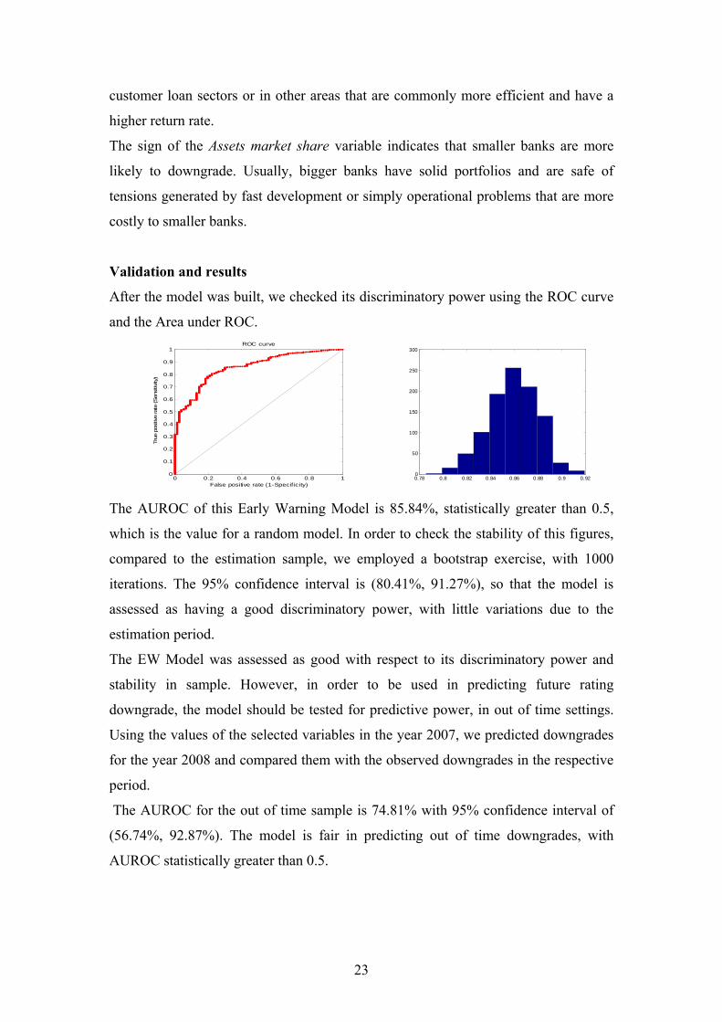
Validation and results

After the model was built, we checked its discriminatory power using the ROC curve

and the Area under ROC.

The AUROC of this Early Warning Model is 85.84%, statistically greater than 0.5,

which is the value for a random model. In order to check the stability of this figures,

compared to the estimation sample, we employed a bootstrap exercise, with 1000

iterations. The 95% confidence interval is (80.41%, 91.27%), so that the model is

assessed as having a good discriminatory power, with little variations due to the

estimation period.

The EW Model was assessed as good with respect to its discriminatory power and

stability in sample. However, in order to be used in predicting future rating

downgrade, the model should be tested for predictive power, in out of time settings.

Using the values of the selected variables in the year 2007, we predicted downgrades

for the year 2008 and compared them with the observed downgrades in the respective

period.

The AUROC for the out of time sample is 74.81% with 95% confidence interval of

(56.74%, 92.87%). The model is fair in predicting out of time downgrades, with

AUROC statistically greater than 0.5.

0.78 0.8 0.82 0.84 0.86 0.88 0.9 0.920

50

100

150

200

250

300

0 0.2 0.4 0.6 0.8 10

0.1

0.2

0.3

0.4

0.5

0.6

0.7

0.8

0.9

1

False positive rate (1-Specificity)

True

pos

itive

rate

(Sen

sitiv

ity)

ROC curve

24

0 0.2 0.4 0.6 0.8 10

0.1

0.2

0.3

0.4

0.5

0.6

0.7

0.8

0.9

1


True

pos

itive

rate

(Sen

sitiv

ity)

ROC curve

Due to the small out of time sample of downgrades, the ROC curve is not concave

and it should be interpreted with care.

The ordered logistic model developed in next section delivers probabilities for each

possible rating so that we can compute a probability of downgrade by adding all the

probabilities for each rating worse than the current value.

The AUROC of this Early Warning Model is 84.87% and the 95% confidence interval

is (79.3%, 90.45%), so that the model is assessed as having a good discriminatory

power, with little variations due to the estimation period. The AUROC for the out of

time sample for this model is 80.39% with 95% confidence interval of (63.6%,

97.17%).

Due to the small out of time sample of downgrades, the respective ROC curve is not

concave and it should be interpreted with care. However, the out of time AUROC

values for the ordered logistic model are higher than those of the binary dependent

variable model, indicating that even though the models perform closely in sample, the

0 0.2 0.4 0.6 0.8 10

0.1

0.2

0.3

0.4

0.5

0.6

0.7

0.8

0.9

1


True

pos

itive

rate

(Sen

sitiv

ity)

ROC curve

0.76 0.78 0.8 0.82 0.84 0.86 0.88 0.9 0.92 0.940

50

100

150

200

250

300

0 0.2 0.4 0.6 0.8 10

0.1

0.2

0.3

0.4

0.5

0.6

0.7

0.8

0.9

1


True

pos

itive

rate

(Sen

sitiv

ity)

ROC curve

25

ordered logistic model predicts more accurate the downgrades of the CAAMPL

Rating in one year horizon.

With respect to the “loss” function of the supervisory authority, the model was used in

order to assess a threshold for a probability of downgrade, which will be, with the

same notation: 2211 )()(minarg ωεωε ×+×= cccc

The weights used for Type I and Type II Errors depend on the importance given by

the supervisory authority to unexpected downgrade events. If this weight is 0.5 the

probability threshold will be 20.2%, where as for the weight of 0.6667 it is 11.0%.

Included observations: 480

Prediction Evaluation (success cutoff C = 0.202)

Estimated Equation Constant Probability

Dep=0 Dep=1 Total Dep=0 Dep=1 Total

P(Dep=1)<=C 319 16 335 403 77 480

P(Dep=1)>C 84 61 145 0 0 0

Total 403 77 480 403 77 480

Correct 319 61 380 403 0 403

% Correct 79.16 79.22 79.17 100.00 0.00 83.96

% Incorrect 20.84 20.78 20.83 0.00 100.00 16.04

Total Gain* -20.84 79.22 -4.79

Percent Gain** NA 79.22 -29.87





P(Dep=1)<=C 283 11 294 0 0 0

P(Dep=1)>C 120 66 186 403 77 480

Total 403 77 480 403 77 480

Correct 283 66 349 0 77 77

% Correct 70.22 85.71 72.71 0.00 100.00 16.04

% Incorrect 29.78 14.29 27.29 100.00 0.00 83.96

Total Gain* 70.22 -14.29 56.67

Percent Gain** 70.22 NA 67.49

26

Using the ordered logistic model presented in the next chapter to estimate

probabilities of rating downgrades, the thresholds will be 18.7% and 11.5%,

respectively. For the first case, the errors will be 19.48% (Type I) and 25.31% (Type

II) and for the second, in which the weight for Type I error is higher, the errors will be

11.69% (Type I) and 36.23% (Type II).

Binary dependent variable model

for probability of downgrade

Ordered logistic Model (see next

section) for probability of downgradeType I

Error

Weight Cutoff Type I

Error

Type II

Error Cutoff

Type I

Error

Type II

Error

50.00% 20.2% 20.78% 20.84% 18.7% 19.48% 25.31%

66.67% 11.0% 14.29% 29.78% 11.5% 11.69% 36.23%

With respect to the probability of downgrade, both types of models can provide useful

results. Generating the Kernel densities for the two models allow us to draw the

following representations for estimation period and for test period.

0

1

2

3

4

5

.0 .1 .2 .3 .4 .5 .6 .7 .8 .9

_PDBIN

Kernel Density (Epanechnikov, h = 0.1099)

0

1

2

3

4

5

0.0 0.1 0.2 0.3 0.4 0.5 0.6 0.7 0.8 0.9 1.0

_PDMULTI


0

2

4

6

8

10

12

.0 .1 .2 .3 .4 .5

_PDBINTEST


0

1

2

3

4

5

6

.0 .1 .2 .3 .4 .5 .6 .7

_PDMULTITEST


27

Comparing the average probabilities of downgrade estimated by the two models, we

find that the ordered logistic model is more conservative to the end of the analyzed

period.

Probability of Downgrade

0.00

0.05

0.10

0.15

0.20

0.25

1 2 3 4 5 6 7 8 9 10 11 12 13 14 15 16 17 18 19 20 21 22 23 24 25

Month

Valu

e Multinomial modelBinary model

5.2. Weak overall position

At this point, we have built a model designed for predicting CAAMPL rating

downgrades, which can be a useful tool in banking supervision. However, this model

should always be doubled by expert opinion and used just as the early warning model

which it is. In fact, the output of the model is a probability of rating downgrade,

without specifying how many grades the downgrade could be and what could be the

probability that the one year horizon rating will be better. A much more useful tool

will be a model that can not only predict rating downgrades, but can also provide a

probability for each possible rating. This issue is particularly helpful as one can obtain

an estimated one year horizon CAAMPL rating, weighting the possible ratings with

their estimated probabilities.

For these reasons we employed an ordered logistic model, considering the theoretical

background presented in the methodology section as well as the general filters used in

the variable selection for rating downgrades. In this case, the variable selection

methodology seeks variables that explain a “bad” future rating in one year horizon.

Kolmogorov – Smirnov Test

Both models have to discriminate between banks with higher ratings and banks with

lower ratings in one year horizon. We used a Kolmogorov – Smirnov test to check

whether the variables fulfill this requirement and we divided the possible ratings into

good (1-2) and bad (3-4) ratings. The test was passed by 40 variables, at a 0.1

threshold for the test p-value. For this mode, we also present a graphic overview of

28

two selected variables – a)ROE(v32) and b)Solvency ratio(v23) – and one rejected

variable – c)Customer loans/Customer deposits(v44):

a) b)

c)

The maximum difference between the distribution of good banks (red line) and bad

banks (blue line) is visibly higher for selected variables compared to the variables

rejected at this step.

Monotony

With respect to monotony, we considered dependent variable takes the value 1 if the

bank will have a bad rating and 0 otherwise, in one year horizon. Similar to the

methodology for predicting probability of downgrade, we used a regression for the

average logarithm odd of the dependent variable with the average of each explanatory

variable, on the ten created subgroups. The number of subgroups was selected

considering the size of the estimation sample and the purpose of building the

monotony test, with limited discrimination, so that to be sure we will not exclude

variables that might perform well in a multivariate framework. We selected a

threshold for p-value at 0.1 and the test showed the a wide variety of values for

selected and rejected variables, like for a)ROE (v32), b)Solvency ratio (v23),

respectively c) Level 1 Own Funds Index (v26).

0 1 2 3 4 5 6 7 8 90

0.1

0.2

0.3

0.4

0.5

0.6

0.7

0.8

0.9

1

x

F(x)

Empirical CDF

FG(x)FB(x)

0 1 2 3 4 5 60

0.1

0.2

0.3

0.4

0.5

0.6

0.7

0.8

0.9

1

x

F(x)

Empirical CDF

FG(x)FB(x)

0 0.1 0.2 0.3 0.4 0.5 0.6 0.7 0.80

0.1

0.2

0.3

0.4

0.5

0.6

0.7

0.8

0.9

1

x

F(x)

Empirical CDF

FG(x)FB(x)

29

a) b)

c)

This test was passed by 24 variables which entered the univariate models.

Univariate framework

The next filter used was similar to the case of the rating downgrade prediction. We

generated univariate logistic models for the tested variables and we set up a threshold

at 0.1 for their p-values. The univariate models assume a dependent variable given by

the one year horizon rating, as 0 for a good rating and 1 for a bad rating. We then

construct logit models with this dependent variable and each tested explanatory

variable and we also check the AUROC for these models. Most of the variables

performed well so that 23 variables passed this test, having only two variables

rejected.

Multicolinearity

Next, the selected variables were analyzed based on their correlations. The competing

variables have been ordered with respect to their AUROC in the univariate models

and then the correlation matrix has been used to eliminate variables with a correlation

higher than the 0.7 threshold when compared to variables with higher univariate

AUROC. However, variables eliminated at this step were highlighted and compared

in model building with the variables they were correlated to.

-0.4 -0.2 0 0.2 0.4 0.6 0.8 10.9

0.95

1

1.05

1.1

1.15

1.2

1.25

1.3

-1 -0.5 0 0.5 1 1.5 20.05

0.1

0.15

0.2

0.25

0.3

0.35

0.4

-1 0 1 2 3 40.8

0.9

1

1.1

1.2

1.3

1.4

1.5

1.6

30

Multivariate models

At this step, we eliminated variables that clearly do not explain the dependent

variable, which in this case is the probability of a bank to be “bad” in one year

horizon.

As presented before for rating downgrades, we build a multivariate binary dependent

variable model for this particular case.

In a backward selection methodology, variables with the highest p-values were

eliminated one at a time, examining the values of the model’s likelihood and Akaike

Information Criterion. If the new model is better, the variable is eliminated and a new

iteration is done.

After several iterations, and after reconsidering the eliminated variables in order to

assess whether they perform better in a multivariate framework. The final binary

dependent variable model, for good/bad banks has the following specifications:


ROE -6.445561 1.655071 -3.894432 0.0001

Rating 1.411898 0.245887 5.742063 0.0000

Loans market share -14.41244 4.445902 -3.241735 0.0012

Solvency ratio 0.630858 0.319149 1.976685 0.0481

General risk rate 2.174651 0.842999 2.579659 0.0099

Consumer price index -0.033098 0.008284 -3.995511 0.0001

Mean dependent var 0.527083 S.D. dependent var 0.499787

S.E. of regression 0.389287 Akaike info criterion 0.931655

Sum squared resid 71.83203 Schwarz criterion 0.983827


Avg. log likelihood -0.453327

The variables selected after the above presented methodology were also introduced in

a multivariate ordered logistic model, with the one year horizon rating being the

dependent variable, which resulted in the following final model:

31


ROE -5.167666 1.449624 -3.564831 0.0004

Rating 1.819074 0.226134 8.044220 0.0000

Loans market share -11.37554 3.144244 -3.617893 0.0003

Solvency ratio 0.455977 0.214223 2.128515 0.0333

General risk rate 2.365373 0.807940 2.927658 0.0034

Limit Points

LIMIT_2:C(6) -2.646104 1.264853 -2.092025 0.0364

LIMIT_3:C(7) 4.883068 0.843593 5.788415 0.0000

LIMIT_4:C(8) 9.216655 0.969939 9.502302 0.0000

Akaike info criterion 1.255066 Schwarz criterion 1.324630


Restr. log likelihood -422.8128 Avg. log likelihood -0.610867

LR statistic (5 df) 259.1938 LR index (Pseudo-R2) 0.306511

Probability(LR stat) 0.000000

These selected variables passed all the tests in a constant manner, having the same

sign both in univariate settings and in multivariate framework.

The dependent variable of this ordered logistic model is the one year horizon rating so

that the variables’ signs have different meaning than in the rating downgrade model.

As expected, the relation between current CAAMPL Rating and the one year horizon

rating is direct so the better the current CAAMPL Rating, the better the one year

horizon rating. This issue can also be explained by the fact that the rating is not so

volatile in time. A bank with strong current position is less likely to be weak in one

year time than a bank that is currently already weak.

Banks with high profitability, as indicated by ROE, are more likely to have a strong

position in one year horizon. The same goes for banks with higher market share

which, due to their size, have the means to properly manage their portfolio in order to

find ways in maintaining a strong overall position.

32

Loans market share affects the future one year rating in the sense banks with higher

market share are less likely to receive a bad rating in one year horizon.

The Solvency ratio for the analyzed banks has always been above the regulatory

threshold therefore its distribution has longer tail on the higher values. Banks with

higher values for the Solvency ratio may have difficulties in finding destinations for

its resources and therefore may be in the situation of having a worse position than

banks with lower but appropriate values of this indicator, due to a weaker

management of resources.

The General risk rate sign indicates that lower risk banks will generally have a higher

probability to have a good (small value) rating in one year horizon. Bad loans and

other assets with high risk weight can easily affect the bank’s situation generating

higher provisions and even losses, in case of defaults.

The influence of the Consumer price index (IPC) on the dependent variable is

negative, meaning that the higher IPC, the lower (therefore better) the one year

horizon rating. For the estimation period, this relation can be observed empirically:

IPC and Average 1Y Rating

2.22.32.42.52.62.72.82.9

1 2 3 4 5 6 7 8 9 10 11 12 13 14 15 16 17

Month

Ave

rage

1Y

Rat

ing

100

105

110

115

120

IPC (%

) Average 1YRating

IPC

During the analyzed period the Consumer price index decreased while the ratings

reached higher values, meaning weaker banks. In the first part of this period the

higher inflation allowed the banks to have higher margins, therefore higher

profitability and stronger position. The last months were characterized by lower

inflation as well as lower profitability, while the banks had to strive more for each

market share point and also for maintaining their sound position. The proc-cyclical

nature of inflation can help us explain this result by connecting economic growth with

inflation and, in the same time, stronger banks. Inflation is also favoring the

reimbursement of loans, decreasing this way the credit risk undertaken by banks. This

33

variable did not enter the ordered logistic model but only the binary dependent

variable model and is therefore useful to analyze both of them.

Validation and results

As it was the case for the first binary dependent variable model for probability of

downgrade, we have also built a ROC curve for this second binary model.

The AUROC of this Early Warning Model is 86.86%, statistically greater than 0.5,

which is the value for a random model. The 95% confidence interval is (83.65%,

90.08%), so that the model is assessed as having a good discriminatory power. The

out of time AUROC for this model is 89.41% with 95% confidence interval of

(83.45%, 95.38%). This method shows that the model has high discriminatory power

with little variations due to the estimation period.

In order to assess the goodness of fit of the ordered logistic model we employed a

ROC based approach, similar to the case of the binary dependent variable model. The

ordered logistic model can target a dependent variable that takes the value 0 for good

banks and 1 for bad banks. Using the calculated probabilities, we can obtain the

estimated probability for a bank to be bad (rating 3-4) and then draw the ROC curve

for this probability and the percentage of banks that were bad in one year horizon.

0.75 0.8 0.85 0.9 0.95 10

50

100

150

200

250

0 0.2 0.4 0.6 0.8 10

0.1

0.2

0.3

0.4

0.5

0.6

0.7

0.8

0.9

1


True

pos

itive

rate

(Sen

sitiv

ity)

ROC curve

0.8 0.82 0.84 0.86 0.88 0.9 0.920

50

100

150

200

250

300

0 0.2 0.4 0.6 0.8 10

0.1

0.2

0.3

0.4

0.5

0.6

0.7

0.8

0.9

1


True

pos

itive

rate

(Sen

sitiv

ity)

ROC curve

34

The AUROC of this Early Warning Model is 86.07% and the 95% confidence interval

is (82.77%, 89.38%), so that the model is assessed as having a good discriminatory

power, with little variations due to the estimation period. The out of time AUROC for

this model is 88.8% with 95% confidence interval of (82.67%, 94.93%).

This method shows that the model has good and stable predicting power.

Considering the models’ in sample performance, we conclude that the binary

dependent variable model does not strongly outperform the ordered logistic model,

which has the advantage of being able to provide probabilities for each possible

rating. This feature may be useful in modeling banks that will have a bad rating in one

year horizon and this model is also well behaved in sample, with high AUROC

values. For this reason, the ordered logistic model may be selected for further use.

However, we tested both models in an out of time setting.

With respect to the “loss” function of the supervisory authority, these models were

also used in order to assess a threshold for a probability of receiving a bad rating. The

weight for Type I Error represents the importance given by the supervisory authority

to unexpected bad ratings events and if this weight is 0.5 the probability threshold will

be 47.5%, where as for the weight of 0.6667 it is 27.2% - for binary dependent

variable model.

0.75 0.8 0.85 0.9 0.95 10

50

100

150

200

250

300

0 0.2 0.4 0.6 0.8 10

0.1

0.2

0.3

0.4

0.5

0.6

0.7

0.8

0.9

1


True

pos

itive

rate

(Sen

sitiv

ity)

ROC curve

0.81 0.82 0.83 0.84 0.85 0.86 0.87 0.88 0.89 0.9 0.910

50

100

150

200

250

0 0.2 0.4 0.6 0.8 10

0.1

0.2

0.3

0.4

0.5

0.6

0.7

0.8

0.9

1


True

pos

itive

rate

(Sen

sitiv

ity)

ROC curve

35





P(Dep=1)<=C 176 49 225 0 0 0

P(Dep=1)>C 51 204 255 227 253 480

Total 227 253 480 227 253 480

Correct 176 204 380 0 253 253

% Correct 77.53 80.63 79.17 0.00 100.00 52.71

% Incorrect 22.47 19.37 20.83 100.00 0.00 47.29

Total Gain* 77.53 -19.37 26.46






P(Dep=1)<=C 129 15 144 0 0 0

P(Dep=1)>C 98 238 336 227 253 480

Total 227 253 480 227 253 480

Correct 129 238 367 0 253 253

% Correct 56.83 94.07 76.46 0.00 100.00 52.71

% Incorrect 43.17 5.93 23.54 100.00 0.00 47.29

Total Gain* 56.83 -5.93 23.75


For ordered logistic model, the probability threshold will be 47.6% and 31.7%,

respectively. For the first case, the errors will be 19.76% (Type I) and 21.59% (Type

II) and for the second, in which the weight for Type I error is higher, the errors will be

10.28% (Type I) and 34.36% (Type II).

36

Binary dependent variable model for

bad future rating

Ordered logistic Model for bad

future rating Type I

Error

Weight Cutoff Type I

Error

Type II

Error Cutoff

Type I

Error

Type II

Error

50.00% 47.5% 19.37% 22.47% 47.6% 19.76% 21.59%

out of time 3.33% 40.74% out of time 5.00% 38.18%

66.67% 27.2% 5.93% 43.17% 31.7% 10.28% 34.36%

out of time 0.00% 64.81% out of time 1.67% 40.00%

The average probabilities estimated for bad future ratings by the two models are

similar, confirming this way that the ordered logistic model is not outperformed and,

therefore, considering the multiple results available through this model, it may be

used in further applications. Probability of Bad Rating

0.0

0.1

0.2

0.3

0.4

0.5

0.6

0.7

0.8

1 2 3 4 5 6 7 8 9 10 11 12 13 14 15 16 17 18 19 20 21 22 23 24 25

Month

Value Multinomial model

Binary model

The probabilities provided by the ordered logistic model for each possible rating can

be used for rating prediction.

Aggregated rating

2.22.32.42.52.62.72.82.9

1 2 3 4 5 6 7 8 9 10 11 12 13 14 15 16 17 18 19 20 21 22 23 24 25

Month

Valu

e EffectivePredicted

Both binary dependent variable and ordered logistic models perform well in sample

and out of time. For the purpose of estimating and predicting rating downgrades, both

of them are useful tools. However, the ordered logistic model has important features

that may recommend it for further analysis and use. The ordered logistic model

provides probabilities for each possible rating and these can be employed to obtain a

rating downgrade probability but also a probability of reaching one particular group of

ratings, such as the top two ratings, or the bottom ones. The discriminatory power of

this model with respect to good/bad banks has proven to be high, so that the ordered

37

logistic model has at least one important supplemental use than the binary dependent

variable model. Also, the simple estimated probabilities can be useful in order to

obtain an estimated rating, as the weight of the possible ratings.

One particular result of the ordered logistic model is rating prediction. In the previous

sections we compared the ordered and binary dependent variable models with respect

to Type I errors and Type II errors for the cutoffs calculated by minimizing the loss

function of the supervisory authority. However, ordered logistic model can also

provide a score for each bank, which can subsequently be transformed in a rating

prediction. We then analyzed whether the banks will have a future weak overall

position or not. For each bank we calculated the Type I errors (E1) as being generated

by unexpected future bad ratings and the Type II errors (E2) as for unexpected future

good ratings. The total error rate is calculated as total errors to number of records, for

each bank.

Bank Code E1 E2

Total error rate

Bank Code E1 E2

Total error rate

1 0.0% 0.0% 0.00% 17 44.4% 8.3% 23.81%2 0.0% 0.0% 0.00% 18 43.8% 60.0% 47.62%3 5.6% 100.0% 19.05% 19 20.0% 45.5% 33.33%4 30.8% 0.0% 19.05% 20 6.3% 80.0% 23.81%5 33.3% 5.6% 9.52% 21 0.0% 0.0% 0.00%6 100.0% 16.7% 28.57% 22 16.7% 100.0% 28.57%7 11.1% 41.7% 28.57% 23 33.3% 26.7% 28.57%8 33.3% 77.8% 52.38% 24 16.7% 100.0% 28.57%9 0.0% 0.0% 0.00% 25 0.0% 0.0% 0.00%

10 100.0% 16.7% 28.57% 26 28.6% 0.0% 19.05%11 50.0% 0.0% 8.33% 27 100.0% 20.0% 23.81%12 16.7% 100.0% 28.57% 28 0.0% 100.0% 14.29%13 35.7% 85.7% 52.38% 30 0.0% 100.0% 23.08%14 0.0% 4.8% 4.76% 33 0.0% 0.0% 0.00%15 22.2% 100.0% 33.33% Total 18.2% 24.6% 21.21%16 0.0% 100.0% 4.76%

The first four banks according to assets market share which hold together 48.75% of

the local banking assets have an average of only 13.1% for total error rate. Banks

numbered 8, 13, 15, 18, and 19 which have the highest total error rate hold together a

market share of 4.84%, being in fact some of the smallest local banks. Banks with

total error rate below 25% account for an assets market share of 69.79%. These results

show that the model performs best for bigger banks and records the highest errors for

some of the smaller credit institutions, while the overall errors are considered to be

acceptable.

38

6. Conclusions

In this paper we aimed to find the determinants for rating downgrades and the ones

for a bank’s future overall position.

After conducting the selection process we obtained two sets of variables that

explained reasonably well the dependent variables, which were related to future rating

downgrades and future bad ratings, respectively. We then generated multivariate

models and after the final models were constructed we were able to highlight the

determinants assumed for the dependent variables.

In this respect, we found that rating downgrades are negatively affected by the current

Rating, ROE and Assets market share, while Loans and deposits placed with other

banks/ Total assets have a positive impact on the probability of downgrade. We note

that all selected variables have the expected influence on downgrades, with only

profitability and assets quality being represented, besides market share and current

position. Capital adequacy and liquidity have no influence in this model, perhaps due

to a higher degree of regulation for the two microeconomic fields which does not

allow for banks to fall under some strict thresholds that are frequently monitored and

set at levels avoiding distress. Macroeconomic environment was also not included in

the model, meaning that the overall position of a Romanian bank is mostly determined

by its characteristics.

Also, an important point of interest was finding the banks that will receive a bad

rating in one year horizon. We found that ROE, Loans market share and Consumer

price index negatively affects the respective probability, while the current Rating,

Solvency ratio and General risk rate have a positive impact. In this case, the model

allows for the influence of profitability, assets quality and capital adequacy, besides

the current position and market share. All variables have the expected signs, with

Solvency ratio signaling an opportunity cost for banks that do not properly manage

their resources. The macroeconomic environment is again found less influential than a

bank’s characteristics, having the Consumer price index only included in the binary

dependent variable model estimating bad future ratings, while the ordered logistic

model keeps all the other variables with the same influence on the future overall

position. These results highlights as well the fact the Romanian banks are dependent

more on their individual business than on macroeconomic elements.

39

With respect to probability estimation, the binary dependent variable models built for

rating downgrades and bad future ratings have not outperformed the ordered logistic

model and all of them had good performance both in sample and out of time, as

shown by AUROC results as well as analyzing Type I and Type II errors for each

model.. The ordered logistic model has the important characteristic of being able to

estimate probabilities for each possible rating and is therefore particularly useful in

rating prediction, providing a score for each bank so that the supervisors are able to

sort the credit institutions based on this criteria. The errors recorded by this model are

acceptable overall, with very good performance for bigger banks, but with significant

errors for some of the smaller banks.

The results generated by the ordered logistic model can be aggregated in order to

obtain an expected rating for banking sector level. This model was able to predict

worse ratings and more downgrades for the end of 2007 and for 2008.

Regarding the value that can be added by an early warning model to the activities run

in banking supervision, we found that both binary dependent variable and ordered

logistic models provide important information about future evolutions and therefore

can be a useful tool in this field. However, the results generated by these models can

also be manipulated trough a consensus method or by analyzing other models and

techniques and they should always be doubled by expert opinion.

This paper provides a framework for building an early warning system regarding the

Romanian banks, as well as for the banking sector as a whole. Therefore this

methodology and subsequent results should be analyzed considering the

characteristics of the local banking sector, which has a small number of banks, mostly

retail oriented, with not enough adverse events to allow for modeling defaults or even

capital inadequacy. Further research with the intended purpose should consider

revising the data set, including new available data based on which the models should

be redeveloped and analyzing other comparable parametric or non-parametric (e.g.

TRA) methods.

40

Bibliography

Altman, E. (1968), “Financial ratios, discriminant analysis and the prediction of

corporate bankruptcy”, The Journal of Finance, 23, 589-609.

Beaver, W. (1966), “Financial ratios as predictors of failure”, Journal of Accounting

Research, 4, 71-111 .

Berger, A. N., M. K. Kyle, and J.M. Scalise (2000), “Did U.S. Bank Supervisors Get

Tougher During the Credit Crunch? Did They Get Easier During the Banking Boom?

Did It Matter to Bank Lending?”, NBER Working Paper no. 7689.

BIS (2002), “Supervisory Guidance on Dealing with Weak Banks”, Basel Committee

on Banking Supervision, Report of the Task Force on Dealing with Weak Banks.

Cashin, P. A. and R. Duttagupta (2008), “The Anatomy of Banking Crises”, IMF

Working Papers,WP/08/93.

Čihák, M. and K. Schaeck (2007), “How Well Do Aggregate Bank Ratios Identify

Banking Problems”, IMF Working Papers, WP/07/275.

Derviz, A. and J. Podpiera (2004), “Predicting Bank CAMELS and S&P Ratings: The

Case of the Czech Republic”, The Working Paper Series of the Czech National Bank

1/2004.

Engelmann, B., E. Hayden and D. Tasche (2003), „Measuring the discriminatory

power of rating systems“, Deutsche Bundesbank, Discussion paper 1.

Gilbert, R. A., A. P. Meyer and M. D. Vaughan (2000), “The Role of a CAMEL

Downgrade Model in Bank Surveillance”, Federal Reserve Bank of St. Louis,

Working Paper 2000-021A.

41

Gilbert, R. A., A. P. Meyer and M. D. Vaughan (2002), “Could a CAMELS

Downgrade Model Improve Off-Site Surveillance?”, Federal Reserve Bank of St.

Louis, Review vol. 84, no.1.

Hammerle, A., R. Rauhmeier and D. Rosch (2003), “Uses and misuses of measures

for credit rating accuracy”, Regensburg University.

Hosmer, D.W. and S. Lemeshow (2000), “Applied Logistic Regression”, John Wiley

& Sons, Inc.

Jagtiani, J., J. Kolari, C. Lemieux and H. Shin (2003), “Early Warning Models for

Bank Supervision: Simpler Could Be Better”, Federal Reserve Bank of Chicago,

Economic Perspectives, Q3.

Kolari, J., D. Glennon, H. Shin and M. Caputo (2000), “Predicting Large U.S.

Commercial Banks Failures”, Journal of Economic and Business 54:361–87.

Ohlson, J. (1980), „Financial ratios and the probabilistic prediction of bankruptcy”,

Journal of Accounting Research, 18, 109-131.

Oshinsky, R. and V. Olin (2006), “Troubled Banks: Why Don't They All Fail?”,

FDIC Banking Review Series, Vol. 18, No. 1, 2006.

Poghosyan, T. and M. Cihák (2009), “Distress in European Banks: An Analysis Based

on a New Dataset”, IMF Working Papers, WP/09/9.

Sahajwala, R. and P. van den Bergh (2000), “Supervisory Risk Assessment and Early

Warning Systems”, BIS, Basel Committee on Banking Supervision Working Papers,

No. 4 – December 2000.

Schuermann, T. (2007), “Credit Migration Matrices”, Federal Reserve Bank of New

York.

42

Wheelock, D., and P. Wilson (2000), “Why do Banks Disappear? The Determinants

of U.S. Bank Failures and Acquisitions”, Review of Economics and Statistics 82, no.

1:127–38.

Worrell, D. (2004), “Quantitative Assessment of the Financial Sector: An Integrated

Approach”, IMF Working Paper, WP/04/153.

43

Annex 1 – Variables and Signs

Variables Code

Downgrade Expected

Sign

Downgrade Emprirical

Sign

“Bad” Bank Expected

Sign

“Bad” Bank Empirical

Sign I. Assets quality

General risk rate (RW exposures/Exposures) v11 + - + +

Customer loans/Total assets v12 - - - - Customer loans/Total

liabilities v13 - - - + Loans and deposits placed

with other banks/ Total assets v14 + + + +

Overdue and doubtful loans/Loans portfolio v15 + + + + Overdue and doubtful

customer loans/Customer loans portfolio (net) v16 + - + -

Overdue and doubtful customer loans/Customer

loans portfolio (gross) v17 Overdue and doubtful

loans/Total assets v18 + + + + Overdue and doubtful loans/Total liabilities v19

Overdue and doubtful loans/Equity v110 + + + +

Overdue and doubtful loans and following debtors

outside the balance sheet/Total assets v111 + + + +

Overdue and doubtful loans and following debtors

outside the balance sheet/Total liabilities v112 + + + +

Customers deposits/Total assets v113 +|- + +|- +

Bank loans//Total liabilities v114 +|- + +|- + Fixed factors/Equity v115

Fixed factors and materials/Total assets v116

Credit risk rate 1 (Exposures…/Loans and

interests...) v117 + + + + Credit risk rate 1a v118 + + + + Credit risk rate 2 v119

Credit risk rate 2a v120 Credit risk rate 3 v121

Credit risk rate 3a v122 Degree of exposures covert

by provisions v123 Substandard, doubtful and

loss loans in equity v124 + + + - Rate of covert doubtful and v125

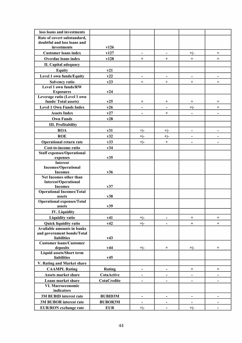
44

loss loans and investments Rate of covert substandard, doubtful and loss loans and

investments v126 Customer loans index v127 - - +|- + Overdue loans index v128 + + + + II. Capital adequacy

Equity v21 Level 1 own funds/Equity v22 - - - -

Solvency ratio v23 + + + + Level 1 own funds/RW

Exposures v24 Leverage ratio (Level 1 own

funds/ Total assets) v25 + + + + Level 1 Own Funds Index v26 - - +|- +

Assets Index v27 - + - - Own Funds v28

III. Profitability ROA v31 +|- +|- - - ROE v32 +|- +|- - -

Operational return rate v33 +|- + - - Cost-to-income ratio v34

Staff expenses/Operational expenses v35 Interest

Incomes/Operational Incomes v36

Net Incomes other than Interest/Operational

Incomes v37 Operational Incomes/Total

assets v38 Operational expenses/Total

assets v39 IV. Liquidity Liquidity ratio v41 +|- - + +

Quick liquidity ratio v42 +|- - + + Available amounts in banks and government bonds/Total

liabilities v43 Customer loans/Customer

deposits v44 +|- + +|- + Liquid assets/Short term

liabilities v45 V. Rating and Market share

CAAMPL Rating Rating - - + + Assets market share CotaActive - - - - Loans market share CotaCredite - - - - VI. Macroeconomic

indicators 3M BUBID interest rate BUBID3M - - - - 3M BUBOR interest rate BUBOR3M - - - - EUR/RON exchange rate EUR +|- - +|- -

45

USD/RON exchange rate USD +|- - +|- - EUR/RON exchange rate

one year variation (%) DEUR +|- - +|- - USD/RON exchange rate one

year variation (%) DUSD +|- - +|- - Net monthly nominal wage SALNOMMEDNET +|- + +|- + Net monthly nominal wage

one year variation (%) Dsal - - - - Consumer price index based

on the same period of last year IPC + - + -

Inflation rate Rinfl + - + - Inflation rate one year

variation Drinfl + + + + Unemployment rate Rsomaj + - + -

Unemployment rate one year variation Dsomaj + + + +

Adjusted unemployment rate Rsomajaj - - + - Adjusted unemployment rate

one year variation Dsomajaj + + + + Industrial production index IPI +|- + +|- +|- Industrial production index

one year variation DIPI +|- + +|- +|- RON Interest rates for non-

governmental assets DA - - - - RON Interest rates for non-

governmental liabilities DP - - - - RON Interest rates for non-

governmental assets one year variation DDA +|- + +|- +

RON Interest rates for non-governmental liabilities one

year variation DDP +|- + +|- +

46

Annex 2 – KS Test

Rating downgrades

Variables KS Sign P-value μND σND μD σD Rating - 0 2.6328 0.606 2.0519 0.4558 v118 + 0.004 0.1522 0.1706 0.1907 0.1778 v117 + 0.0041 0.1495 0.1696 0.1826 0.1733

CotaCredite - 0.0077 0.0389 0.071 0.0158 0.0193 v23 + 0.0136 0.3608 0.4485 0.5332 0.9065 v14 + 0.0159 0.3321 0.1394 0.3786 0.1541

CotaActive - 0.0161 0.0365 0.0625 0.0151 0.0168 v25 + 0.0196 0.1535 0.1059 0.1692 0.094 v42 - 0.0459 0.5662 1.3346 0.562 0.271 v13 - 0.0552 0.6178 0.1999 0.5692 0.1961 DIPI + 0.0631 4.9278 4.2525 6.3078 4.3955

v12 - 0.1091 0.4833 0.1521 0.4476 0.1617 v16 - 0.1091 0.4833 0.1521 0.4476 0.1617 v22 - 0.1385 1.4952 0.7511 1.467 0.7001 v41 - 0.1399 2.9475 2.4682 2.2699 0.8956 IPC - 0.1471 111.0263 3.7588 110.314 3.8235 Rinfl - 0.1471 11.0263 3.7588 10.314 3.8235 IPI + 0.1471 124.4839 8.4145 126.1792 9.3899 DA - 0.1471 24.3609 6.6304 23.0814 7.2268

EUR - 0.1598 3.7449 0.2338 3.7167 0.2474 USD - 0.1748 3.0906 0.2425 3.0408 0.2563 Dsal - 0.1748 0.2307 0.0349 0.2217 0.0414 v18 + 0.2541 0.0028 0.0041 0.0031 0.0045 v112 + 0.2541 0.0028 0.0041 0.0031 0.0045 DDP + 0.2904 -5.1913 5.8565 -4.3 5.7445 v110 + 0.3077 0.017 0.0235 0.018 0.0253 v114 + 0.3077 0.017 0.0235 0.018 0.0253

SALNOMMEDNET + 0.3231 672.6843 170.1884 708.1593 179.0915

Dsomajas + 0.3257 -1.1387 1.0169 -0.9473 0.9754 Dsomaj + 0.3431 -1.1538 1.1021 -0.9623 1.0574

v113 + 0.3786 0.0036 0.0061 0.004 0.0057 v26 - 0.3821 1.0605 0.3141 1.0197 0.0661 v124 + 0.4103 0.053 0.0654 0.0584 0.0805

BUBOR3M - 0.4338 15.045 5.8158 14.2274 5.7848 DP - 0.4338 11.6378 4.2026 11.0924 4.4311

v127 - 0.4851 1.1356 1.6863 1.031 0.0792 v27 + 0.4871 1.052 0.1195 1.059 0.1004

DEUR - 0.5208 0.0409 0.1275 0.0311 0.1201 Rsomaj - 0.5208 6.4764 1.0673 6.3377 1.0994

Rsomajaj - 0.5208 6.4513 0.9523 6.2942 0.9716 v11 - 0.5797 0.4992 0.1545 0.4753 0.163

v15 + 0.6193 0.0051 0.009 0.006 0.0105 v111 + 0.6535 0.0053 0.0095 0.0063 0.0108 DDA + 0.7276 -7.6081 5.7691 -7.0432 5.5463

47

v128 + 0.8229 2.146 10.5955 45.4507 388.5757 v44 + 0.9851 1.2174 1.0213 1.2606 1.1886

BUBID3M - 0.9863 12.0101 5.0432 11.5815 4.9493 Drinfl + 0.9893 -4.3363 3.0626 -4.1535 3.1044 DUSD - 0.9992 -0.0368 0.0702 -0.0386 0.0705

Bad Ratings

Variables KS Sign P-value μGOOD σGOOD μBAD σBAD

v117 + 0 0.1312 0.1679 0.1759 0.1702v118 + 0 0.131 0.1675 0.183 0.1729v22 - 0 1.8194 0.8042 1.1958 0.5322v23 + 0 0.2901 0.321 0.4767 0.6837v25 + 0 0.1241 0.0824 0.1847 0.1131v31 - 0 0.0222 0.0122 0.0108 0.0133v32 - 0 0.1691 0.1084 0.0601 0.0712v33 - 0 1.2188 0.1688 1.0852 0.179CotaActive - 0 0.0539 0.0764 0.0144 0.0211CotaCredite - 0 0.0596 0.0876 0.0133 0.0199Rating + 0.0000 2.1938 0.4954 2.8498 0.5574v11 + 0.0004 0.4716 0.1477 0.5167 0.1603v42 + 0.0041 0.4682 0.2912 0.6529 1.6647v124 - 0.0045 0.0549 0.0614 0.0529 0.0736IPC - 0.0206 111.4571 3.7126 110.423 3.7695Rinfl - 0.0206 11.4571 3.7126 10.4229 3.7695v12 - 0.0207 0.4936 0.1446 0.4632 0.161v16 - 0.0207 0.4936 0.1446 0.4632 0.161USD - 0.0235 3.1179 0.2336 3.0509 0.2514v26 + 0.0257 1.0427 0.164 1.0642 0.3672DIPL + 0.0391 4.6207 4.2182 5.6233 4.3276BUBOR3M - 0.0442 15.5966 5.7718 14.3013 5.792SALNOMMEDNET + 0.0442 653.5084 162.1538 700.686 177.659IPL + 0.0442 123.6079 8.2405 125.786 8.7821DA - 0.0442 25.0948 6.4587 23.313 6.8835DP - 0.0442 12.0393 4.1486 11.1116 4.2812v14 + 0.0448 0.3308 0.1332 0.3474 0.1506v111 + 0.0486 0.0045 0.0078 0.0063 0.0111v13 + 0.0524 0.5994 0.171 0.6195 0.2226v113 + 0.0586 0.0028 0.0036 0.0044 0.0075v15 + 0.0598 0.0042 0.0065 0.0062 0.011v27 - 0.0598 1.0533 0.1399 1.053 0.091v18 + 0.0618 0.0023 0.0029 0.0032 0.0051v112 + 0.0618 0.0023 0.0029 0.0032 0.0051DEUR - 0.0676 0.0522 0.1302 0.0277 0.1218Rsomajaj - 0.0676 6.5553 0.9433 6.3102 0.9546Rsomaj - 0.0965 6.5841 1.0765 6.3375 1.0575v127 + 0.1014 1.0419 0.1064 1.1878 2.1262EUR - 0.1147 3.7605 0.2345 3.7223 0.2363BUBID3M - 0.1468 12.4431 5.0289 11.4911 4.9897Dsal - 0.2374 0.2323 0.033 0.2266 0.0386

48

v128 + 0.252 2.5653 13.5224 14.9495 214.384v110 + 0.2794 0.0169 0.0214 0.0174 0.0258v114 + 0.2794 0.0169 0.0214 0.0174 0.0258Dsomaj + 0.2864 -1.207 1.1618 -1.0478 1.0303DUSD - 0.2931 -0.0322 0.0683 -0.0415 0.0718v41 + 0.3741 2.5605 1.2151 3.0885 2.9362DDP + 0.4412 -5.4675 6.0119 -4.6722 5.6707v44 + 0.4524 1.1285 0.8249 1.3103 1.2102Drinfl + 0.4749 -4.5006 3.1548 -4.1332 2.9813Dsomajas + 0.5082 -1.1875 1.0677 -1.0367 0.9553DDA + 0.6387 -7.8104 5.953 -7.2547 5.5249

49

Annex 3 – Monotony

Rating downgrades

Variable coef p-value Rating -1.7409 0.0006 CotaCredite -11.3279 0.0024 DIPI 0.1141 0.0051 CotaActive -13.2768 0.0058 v14 2.2828 0.0075 v116 -0.8048 0.0084 v115 -0.7939 0.0146 v41 -0.1854 0.0422 DDP 0.0488 0.0532 DDA 0.0407 0.0723 v25 2.1703 0.0897 Dsomajas 0.3245 0.0903

Bad ratings

Variable coef p-value Rating 2.2739 0.0000SALNOMMEDNET 0.0018 0.0000v42 0.9990 0.0003USD -1.1574 0.0003v32 -14.5245 0.0005v22 -1.3865 0.0008DA -0.0394 0.0014v25 7.6877 0.0018IPI 0.0345 0.0038v31 -75.2235 0.0039Rinfl -0.0723 0.0050IPC -0.0723 0.0050Rsomajaj -0.2365 0.0057BUBOR3M -0.0403 0.0068DP -0.0536 0.0096v33 -6.1236 0.0100DIPI 0.0460 0.0168Rsomaj -0.2219 0.0173CotaCredite -14.3810 0.0175v23 1.2082 0.0201v27 2.8107 0.0337DEUR -1.6693 0.0451CotaActive -15.6301 0.0478v11 2.2591 0.0482v113 56.9773 0.0942

50

Annex 4 – Univariate Framework

Rating downgrades

Variable Coefficient Std. Error z-Statistic Prob. AUC Rating -2.1230 0.3256 -6.5203 0.0000 0.7403 v14 2.0470 0.7915 2.5862 0.0097 0.6016 DIPI 0.0729 0.0285 2.5607 0.0104 0.5888 CotaCredite -12.2136 4.9837 -2.4507 0.0143 0.5753 CotaActive -15.0029 5.4122 -2.7721 0.0056 0.5565

Bad ratings

Variable Coefficient Std. Error z-Statistic Prob. AUC v32 -12.8598 1.2220 -10.5234 0.0000 0.8129 Rating 2.4656 0.1931 12.7719 0.0000 0.7820 CotaCredite -20.1209 3.5301 -5.6998 0.0000 0.7677 CotaActive -20.0159 3.1546 -6.3449 0.0000 0.7596 v31 -65.9501 7.7643 -8.4940 0.0000 0.7558 v22 -1.4853 0.1657 -8.9628 0.0000 0.7459 v33 -4.4319 0.5853 -7.5715 0.0000 0.7323 v25 5.2074 0.9319 5.5878 0.0000 0.6636 v23 0.4846 0.1622 2.9875 0.0028 0.6480 v11 2.0933 0.5821 3.5962 0.0003 0.5950 IPC -0.0762 0.0241 -3.1549 0.0016 0.5853 Rinfl -0.0762 0.0241 -3.1549 0.0016 0.5853 DA -0.0422 0.0134 -3.1379 0.0017 0.5815 SALNOMMEDNET 0.0017 0.0005 3.2243 0.0013 0.5781 USD -1.1616 0.3695 -3.1434 0.0017 0.5770 Rsomajaj -0.2799 0.0949 -2.9486 0.0032 0.5756 IPI 0.0316 0.0106 2.9913 0.0028 0.5731 DIPI 0.0551 0.0210 2.6266 0.0086 0.5727 Rsomaj -0.2273 0.0847 -2.6834 0.0073 0.5701 BUBOR3M -0.0401 0.0155 -2.5907 0.0096 0.5637 DP -0.0552 0.0212 -2.6060 0.0092 0.5607 DEUR -1.5894 0.7142 -2.2254 0.0261 0.5495 v113 34.6881 14.4214 2.4053 0.0162 0.5487

51

Annex 5 – Multicolinearity

Rating downgrades

AUC UV PD Rating v31 v14 v32 DIPL Cota

Credite Cota

Active 0.7403 Rating 1.000 -0.576 -0.070 -0.573 0.013 -0.301 -0.284 0.6863 v31 -0.576 1.000 -0.006 0.788 -0.161 0.258 0.261 0.6017 v14 -0.070 -0.006 1.000 0.009 -0.007 -0.086 -0.001 0.5946 v32 -0.573 0.788 0.009 1.000 -0.154 0.321 0.358 0.5888 DIPI 0.013 -0.161 -0.007 -0.154 1.000 -0.002 -0.008 0.5753 CotaCredite -0.301 0.258 -0.086 0.321 -0.002 1.000 0.964 0.5562 CotaActive -0.284 0.261 -0.001 0.358 -0.008 0.964 1.000

Bad ratings

Variable AUROC UV IPC IPC 0.59 1.00Rinfl 0.59 1.00DA 0.58 0.89SALNOMMEDNET 0.58 -0.93USD 0.58 0.88Rsomajaj 0.58 0.98IPI 0.57 -0.84Rsomaj 0.57 0.92BUBOR3M 0.56 0.81DP 0.56 0.80DEUR 0.55 0.89

Variable AUROC UV v32 v32 0.81 1.00 v31 0.76 0.79

Early Warning Models for Banking Supervision in Romania papers/Muntean Radu/muntean.radu... ·...

Documents

Transcript of Early Warning Models for Banking Supervision in Romania papers/Muntean Radu/muntean.radu... ·...