EARLY ONLINE RELEASE - JST

EARLY ONLINE RELEASE

This is a PDF of a manuscript that has been peer-reviewed

and accepted for publication. As the article has not yet been

formatted, copy edited or proofread, the final published

version may be different from the early online release.

This pre-publication manuscript may be downloaded,

distributed and used under the provisions of the Creative

Commons Attribution 4.0 International (CC BY 4.0) license.

It may be cited using the DOI below.

The DOI for this manuscript is

DOI:10.2151/jmsj. 2018-035

J-STAGE Advance published date: April 8th, 2018

The final manuscript after publication will replace the

preliminary version at the above DOI once it is available.

1

Assimilation and Forecasting Experiment for Heavy 2

Siberian Wildfire Smoke in May 2016 with Himawari-8 3

Aerosol Optical Thickness 4

5

Keiya YUMIMOTO1, 2, Taichu Y. TANAKA2, Mayumi YOSHIDA3, 6

Maki KIKUCHI3, Takashi M. NAGAO3, Hiroshi MURAKAMI3, 7

and Takashi MAKI2 8

9

1 Research Institute for Applied Mechanics, Kyushu University, Kasuga-city, Fukuoka 816-10

8580, Japan. 11

2 Meteorological Research Institute, Japan Meteorological Agency, Tsukuba, Ibaraki 305-12

0052, Japan. 13

3 Earth Observation Research Center, Japan Aerospace Exploration Agency, Tsukuba, 14

Ibaraki, Japan. 15

16

17

18

May 18, 2017 19

20

21

22

23

------------------------------------ 24

1) Corresponding author: Keiya Yumimoto, Research Institute for Applied Mechanics, 25

Kyushu University, 6-1 Kasugakoen, Kasuga-city, Fukuoka 816-8580, JAPAN. 26

Email: [email protected] 27

Tel: +81-92-583-7772 28

Fax: +81-92-583-7774 29

30

1

Abstract (< 300 words) 31

The Japan Meteorological Agency (JMA) launched a next-generation geostationary 32

meteorological satellite (GMS), Himawari-8, on October 7, 2014 and began its operation on 33

July 7, 2015. The Advanced Himawari Imager (AHI) onboard Himawari-8 has 16 34

observational bands that enable the retrieval of full-disk maps of aerosol optical properties 35

(AOPs), including aerosol optical thickness (AOT) and the Ångström exponent (AE) with 36

unprecedented spatial and temporal resolution. In this study, we combined an aerosol 37

transport model with the Himawari-8 AOT using the data assimilation method, and 38

performed aerosol assimilation and forecasting experiments on smoke from an intensive 39

wildfire that occurred over Siberia between May 15 and 18, 2016. To effectively utilize the 40

high observational frequency of Himawari-8, we assimilated 1-h merged AOTs generated 41

through the combination of six AOT snapshots taken over 10-min intervals, three times per 42

day. The heavy smoke originating from the wildfire was transported eastward behind a low-43

pressure trough, and covered northern Japan from May 19 to 20. The southern part of the 44

smoke plume then traveled westward, in a clockwise flow associated with high pressure. 45

The forecast without assimilation reproduced the transport of the smoke to northern Japan; 46

however, it underestimated AOT and the extinction coefficient compared with observed 47

values, mainly due to errors in the emission inventory. Data assimilation with the Himawari-48

8 AOT compensated for the underestimation and successfully forecasted the unique C-49

shaped distribution of the smoke. In particular, the assimilation of the Himawari-8 AOT during 50

2

May 18 greatly improved the forecast of the southern part of the smoke flow. Our results 51

indicate that the inheritance of assimilation cycles and the assimilation of more recent 52

observations led to better forecasting in this case of a continental smoke outflow. 53

54

Keywords Aerosol; aerosol transport model; data assimilation; Himawari-8; wildfire 55

smoke 56

57

3

1. Introduction 58

Airborne aerosols play an important role in air quality and human health. The World Health 59

Organization (WHO) has suggested that 6.5 million deaths per year may be associated with 60

air pollution exposure and its health impact (WHO, 2016). It is well known that aerosols 61

affect Earth’s radiation budget by scattering and absorbing radiation (direct effect) and 62

modifying the cloud properties (indirect effect). This aerosol effect on the radiation balance 63

is crucial not only for estimating climate change (i.e., long-range effects; IPCC, 2013) but 64

also for weather prediction (i.e., short-range effects). Various studies have reported the 65

influence of accurate simulation of aerosols and their radiative effects on the accuracy of 66

numerical weather prediction (NWP) (e.g., Rodwell and Jung 2008; Grell and Baklanov 67

2011; Morcrette et al. 2011; Mulcahy et al. 2014; Toll et al. 2016). For example, Pérez et al. 68

(2006) took the radiative effects of African mineral dust into account and showed an 69

improvement in temperature and mean sea-level pressure forecasts. Grell et al. (2011) 70

applied the chemistry version of the Weather Research and Forecasting (WRF-Chem) 71

model to intense wildfires during the 2004 Alaska wildfire season and found that the 72

interaction of aerosols from wildfires with atmospheric radiation led to significant 73

modifications in vertical temperature and moisture profiles. 74

To monitor air quality, provide early warning of heavy pollution events, and improve the 75

accuracy of NWP, operational forecasting centers have been developing and operating 76

aerosol forecasting systems that forecast the three-dimensional (3D) distribution of aerosols. 77

4

To share best practices and discuss pressing issues facing the operational aerosol 78

community, multi-model inter-comparison projects, including the International Cooperative 79

for Aerosol Prediction (ICAP; Sessions et al. 2015), and the World Meteorological 80

Organization (WMO) Sand and Dust Storm Warning Advisory and Assessment System 81

(SDS-WAS; Terradellas et al. 2015) were established by operational forecasting centers. 82

Variation in multi-model forecasting indicated that large uncertainties remained in aerosol 83

forecasting, requiring further research for improved accuracy (Sessions et al. 2015). To this 84

end, data assimilation techniques have been incorporated into aerosol transport models to 85

obtain better initial conditions for forecasting. Both variation-based methods (e.g., Benedetti 86

et al. 2009; Zhang et al. 2008; Wang and Niu 2013) and ensemble-based methods (e.g., Di 87

Tomaso et al. 2016; Rubin et al. 2016; Yumimoto et al. 2016a) have been used by 88

forecasting centers. More recently, Rubin et al. (2017) performed assimilation and 89

forecasting experiments to determine aerosol optical thickness (AOT) from ground- and 90

satellite-based observations with the Navy Aerosol Analysis Prediction System (NAAPS) 91

using two-dimensional variation (2D-var) methods and ensemble-based assimilation 92

systems; their study results showed that ensemble-based assimilation is a more suitable 93

method for incorporating spatially sparse observations (i.e., ground-based networks) than 94

2D-var assimilation. 95

The Meteorological Research Institute (MRI) of the Japan Meteorological Agency (JMA) 96

has developed an online aerosol transport model coupled with an atmospheric general 97

5

circulation model (AGCM), the Model of Aerosol Species IN the Global AtmospheRe 98

(MASINGAR; Tanaka and Chiba 2005). JMA has been using MASINGAR for operational 99

sand and dust storm forecasting since January 2004. Recently, JMA launched Himawari-8, 100

the eighth Japanese geostationary meteorological satellite (GMS) on October 7, 2014 and 101

started its operation on July 7, 2015. The Advanced Himawari Imager (AHI) onboard 102

Himawari-8 has 16 observational bands over the visible and infrared wavelength range, with 103

higher spatial (0.5–2 km) and temporal (full-disk image every 10 min) resolution compared 104

with those of previous GMSs (Bessho et al. 2016). Particularly, the three visible bands (0.47, 105

0.51, and 0.64 μm) and one near-infrared (0.86 μm) band are sensitive to aerosol scattering 106

and absorption, and enable the retrieval of aerosol optical properties (AOPs) including AOT 107

and the Ångström exponent (AE) over wide areas of Asia and Oceania with unprecedented 108

frequency from geostationary orbit. 109

Our research team previously developed an aerosol data assimilation and forecasting 110

system based on MASINGAR mk-2 and an ensemble-based assimilation technique called 111

the Local Ensemble Transform Kalman Filter (LETKF; Hunt et al. 2007), and have reported 112

successful results with AOPs from the Moderate Resolution Imaging Spectroradiometer 113

(MODIS) and Himawari-8 (Yumimoto et al. 2016b,a). However, the ensemble-based 114

assimilation system has a relatively high computational cost, and the development of 115

operational and quasi-real-time aerosol forecasting remains unrealistic. Therefore, in 116

addition to the ensemble-based system, we developed an aerosol data assimilation and 117

6

forecasting system based on the 2D-Var method called MASINGAR/2D-Var (Yumimoto et 118

al. 2017) for operational assimilation and forecasting. 119

In this study, we present the integration of MASINGAR mk-2 and the Himawari-8 AOPs 120

through the 2D-Var assimilation to improve aerosol forecasting. Assimilation and forecasting 121

experiments were performed targeting smoke from a severe wildfire that occurred over 122

Siberia from May 15–18, 2016 (the east side of Lake Baikal). The aerosol model, the data 123

assimilation system, the observational data used in assimilation and validation, and the 124

experimental conditions are outlined in Section 2. In Section 3, we briefly describe the 125

emission and transport of smoke. Section 4 presents the assimilation and forecasting results 126

and the results of their validation. Finally, conclusions are summarized in Section 5. 127

128

2. Methods, observations, and experimental setting 129

2.1 Aerosol transport model 130

We used MASINGAR mk-2, which is the first major update of the global aerosol transport 131

model MASINGAR developed at MRI/JMA. MASINGAR mk-2 covers the major tropospheric 132

aerosol components (i.e., black and organic carbon, mineral dust, sea salt, and sulfate 133

aerosols) and their precursors (e.g., sulfur dioxide and dimethyl sulfide), and is coupled 134

online with an atmospheric general circulation model (MRI-AGCM3; Yukimoto et al. 2012). 135

MASINGAR mk-2 took over from the original MASINGAR for operational sand and dust 136

forecasts as of November 2014, and serves as a member of the ICAP multi-model ensemble 137

7

(Sessions et al. 2015). Emissions of mineral dust and sea salt aerosols are calculated online 138

using schemes developed by Shao et al. (1996) and Gong (2003), respectively. We used 139

the MACCity (MACCC/City ZEN EU projects) emission inventory 140

(http://ether.ipsl.jussieu.fr/eccad) and the Global Fire Assimilation System (GFAS) data set 141

(http://www.gmes-atmosphere.eu/about/project_structure/input_data/d_fire) for 142

anthropogenic and biomass burning emissions, respectively. More detailed information 143

about MASINGAR mk-2 can be obtained in Yumimoto et al. (2017) and Yukimoto et al. 144

(2012). 145

146

2.2 Data assimilation system 147

The cost function in the 2D-Var method is defined as 148

𝐽𝜏(𝝉) =1

2(𝝉 − 𝝉𝑓)

𝑇𝐏𝜏−1(𝝉 − 𝝉𝑓) +

1

2(𝝉𝑜 −𝐇𝐼𝝉)

𝑇𝐑−1(𝝉𝑜 − 𝐇𝐼𝝉), (1) 149

where τ denotes the modeled AOT vector (a two-dimensional diagnostic variable); the suffix 150

f represents the first guess (a priori); τo denotes a vector that contains observed AOT used 151

for the assimilation; Pτ and R are the background error covariance matrix for AOT and the 152

observation error covariance matrix, respectively; and HI is the interpolation into observation 153

space and a linear operator. The analysis increment of AOT (δτa) is derived from Eq. 1 as 154

𝛿𝝉𝑎 = 𝝉𝑎 − 𝝉𝑓 = 𝐊(𝝉𝑜 − 𝐇𝐼𝝉𝑓), (2) 155

where τa is the analysis (a posteriori) ΑΟΤ, which provides the minimum of the cost function; 156

(𝝉𝑜 −𝐇𝐼𝝉𝑓) is the innovation; and K is the Kalman gain, defined as 157

http://www.gmes-atmosphere.eu/about/project_structure/input_data/d_fire

8

𝐊 = 𝐏𝜏 𝐇𝐼𝑇(𝐑+𝐇𝐼𝐏𝜏 𝐇𝐼

𝑇)−1

. (3) 158

Because the Himawari-8 AOT is a column-integrated variable and includes no information 159

about the vertical profile or the aerosol component, the analysis increment of AOT (δτa) is 160

allocated into the aerosol mass mixing ratio, keeping the shape of the vertical profile and 161

the contribution of each aerosol component in the first guess aerosol fields as 162

𝛿𝒙𝑙,𝑘𝑎 = 𝛿𝝉𝑙

𝑎 𝒙𝑙,𝑘𝑓

𝜶𝑙,𝑘𝑓

𝜶𝑙,𝑘𝑓

𝝉𝑓, (4) 163

where 𝛿𝒙𝑙,𝑘𝑎 is the analysis increment of the mixing ratio of the l-th aerosol component and 164

the k-th vertical layer, and 𝒙𝑙,𝑘𝑓

and 𝜶𝑙,𝑘𝑓

represent the first-guess mixing ratio and the 165

extinction coefficient of the l-th aerosol component and k-th vertical layer, respectively. 166

Finally, the analysis (a posteriori) mixing ratio (𝒙𝑙,𝑘𝑎 ) is given by 167

𝒙𝑙,𝑘𝑎 = 𝒙𝑙,𝑘

𝑓+ 𝛿𝒙𝑙,𝑘

𝑎 . (5) 168

Yumimoto et al. (2017) provides a detailed description of MASINGAR/2D-Var. 169

To include observed information, forecasting is initialized by the analysis (a posteriori) 170

aerosol field. The timeline for the operational assimilation and forecasting is shown in Fig. 1. 171

One cycle consists of a 1-day analysis run and a 5-day forecasting run. During the analysis 172

run, the model experiences data assimilation with observations. We performed assimilations 173

three times during the daytime of East Asia (at 03:00, 06:00, and 00:00 Universal Time 174

(UTC)) with the Himawari-8 AOT in the analysis run. The 5-day forecasting was then 175

initialized with the results of the analysis run. In the subsequent cycle, the assimilation run 176

used the results from the previous analysis run as the initial condition. 177

9

Background error covariance is an important parameter that weights the first term of the 178

cost function (Eq. 1) and propagates observed information to regions far from the observed 179

point through its non-diagonal components (i.e., correlation). In this study, we developed a 180

method similar to the National Meteorological Center (NMC) method (Parrish and Derber 181

1992), and defined the background error covariance between model grids m and n (i.e., the 182

(m, n) element of the covariance matrix) as 183

𝑃𝑚,𝑛 =1

𝑁−1∑ (𝜏𝑚

𝑓− 𝜏𝑚,𝑖)

𝑁𝑖=1 𝐶𝑚,𝑛(𝜏𝑛

𝑓− 𝜏𝑛,𝑖), (6) 184

where τm and τn are AOT at model grid m and n; f refers to the first guess; i refers to the ith 185

ensemble member; N is the number of the ensemble; Cm,n is the smooth weighting function. 186

To prevent a spurious large covariance between distant model grids, we introduced the 187

smooth weighting function Cm,n, whose value diminishes as the distance between model 188

grids increases, and a localization technique (Yumimoto et al., 2017). We employed the 189

second-order auto-regressive (SOAR) approximation (Daley and Barker 2001) to calculate 190

the value of Cm,n: 191

𝐶𝑚,𝑛 = (1 +𝑅𝑚,𝑛

𝐿)exp (1 +

𝑅𝑚,𝑛

𝐿), (7) 192

where Rm,n denotes the distance (km) between model grids m and n, and L is the horizontal 193

error correlation length. The localization technique divides the model space into local regions 194

using a prescribed localization scale to reduce spurious error covariance with distance and 195

enables parallel processing to be used to reduce computational cost. The AOT ensemble 196

(τm,i and τn,I, i = 1,…,N) was collected from AOT values within ±5 h of the targeted hour of the 197

10

five previous forecasts. For example, for assimilation at 06 UTC on May 18, AOT values at 198

01:00, 02:00, 03:00, 04:00, 05:00, 06:00, 07:00, 08:00, 09:00, 10:00, and 11:00 UTC on May 199

18 from forecasts started on May 14, 15, 16, 17, and 18 were assigned as the AOT ensemble. 200

In this case, the ensemble number is 55 (11 × 5). 201

Figure 2 shows examples of variance and covariance at 00 UTC on May 18 and 19. 202

Distributions of covariance (Figs. 2c and 2f) were similar to those of the wildfire smoke 203

represented by the first guess AOT (Figs. 2a and 2d). In the case of May 18 (Fig. 2, upper 204

panels), the aerosol plume around 45°N, 136°E has a relatively large correlation with 205

another aerosol plume around 47°N, 126°E (approximately 800 km apart). This result implies 206

that both plumes originated from the same source. 207

208

2.3 Observation data 209

a. Himawari-8 data 210

The AOT retrieved from AHI onboard Himawari-8 was used for the assimilation. The Earth 211

Observing Research Center (EORC) of the Japan Aerospace Exploration Agency (JAXA) 212

processes Himawari-8 data and provides Himawari-8 AOPs via the JAXA Himawari Monitor 213

(http://www.eorc.jaxa.jp/ptree/index.html). Through this system, two levels of AOP products 214

(L2 and L3 products) are available. The L2 product includes full-disk AOT and AE at a 215

wavelength of 500 nm every 10 min. Details of the AOP retrieval algorithm for the L2 product 216

are provided in Yoshida et al. (2017). The L3 product consists of hourly AOPs derived from 217

11

a combination of the 10-min AOPs (L2 product). Taking advantage of Himawari-8’s high-218

frequency observations, the combination enables minimization of the number of pixels 219

missing due to cloud and sunglint and removes degradation due to cloud contamination. 220

Figure 3 shows a map of AOT from the L2 product and merged AOT from the L3 product at 221

03 UTC on May 19, 2016. Details of the combined algorithm for the L3 product are provided 222

in Kikuchi et al. (2018). In this study, to efficiently utilize high-frequency Himawari-8 223

observations, we applied merged AOT in the L3 product (Version 1.0) as assimilation data. 224

Because only AOT at 550 nm is not available in the current version of the system, we 225

extrapolated the merged AOTs at 500 nm into AOTs at 550 nm using the AE of the L3 product. 226

The extrapolated AOTs were averaged in the model grid, and then used in assimilation. We 227

also used wildfire detection data provided by the JAXA Himawari Monitor to identify the 228

source region of the wildfire smoke. 229

b. Validation data 230

We used observation data from satellite-based and ground-based measurements that 231

were not used in the data assimilation to analyze the wildfire smoke and validate the 232

forecasting results. MODIS onboard Terra and Aqua low Earth orbit (LEO) satellites provide 233

AOPs once per day (at approximately 10:30 local time (LT) for Terra and approximately 234

13:30 LT for Aqua). We used the “optical depth land and ocean mean” contained in the 235

Collection 6.0 L2 aerosol data (Levy et al. 2013, 2015). Lidar observations provide vertical 236

profiles of suspended layers in the wildfire smoke. Cloud-Aerosol Lidar with Orthogonal 237

12

Polarization (CALIOP), onboard the Cloud-Aerosol Lidar and Infrared Pathfinder Satellite 238

Observation (CALIPSO) satellite, is a space-based backscatter Lidar instrument launched 239

April 28, 2006 that provides continuous global observations of aerosol and cloud vertical 240

distributions (Winker et al. 2010). We used attenuated backscatter coefficient profiles at 532-241

nm from the Level 1B product (Version 3.30) and the aerosol subtype from the Level 2 242

product (Version 3.30). The Asian Dust and Aerosol Lidar Observation Network (AD-Net), 243

operated by the National Institute for Environmental Studies (NIES), distributes Mie Lidar at 244

20 ground-based stations over East Asia and continuously measures the vertical distribution 245

of aerosols (Sugimoto et al. 2008; http://www-lidar.nies.go.jp). Aerosol extinction coefficients 246

observed at 532 nm at Sendai (38.25°N, 140.85°E), Niigata (37.84°N, 138.94°E), and 247

Matsue (35.21°N, 133.01°E) were applied to analysis of the wildfire smoke and validation of 248

the forecasting results. AOT observations from the Aerosol Robotic Network (AERONET; 249

Holben et al. 1998; https://aeronet.gsfc.nasa.gov) were used to validate assimilation and 250

forecasting results. We compared AOT at 550 nm, extrapolated from AOT at 500 and 640 251

nm through the Ångström law at Hokkaido_University (43.08°N, 141.34°E) and Niigata, with 252

modeled values. The locations of the stations are shown in Fig. 4. To trace the pathway and 253

identify the origin of the wildfire smoke, we used the National Oceanic and Atmospheric 254

Administration (NOAA) Hybrid Single-Particle Lagrangian Integrated Trajectory model 255

(HYSPLIT; http://ready.arl.noaa.gov/HYSPLIT.php; Stein et al. 2015), driven by 256

meteorological data from the Global Data Assimilation System (GDAS) 0.5 degree archive. 257

13

2.4 Experimental conditions 258

To estimate the impact of data assimilation with the Himawari-8 AOPs on the forecast of 259

wildfire smoke, we performed one free run without assimilation (hereafter referred to as 260

noDA) and two cycles of assimilation and forecast runs (Fig. 1). The first cycle (DA1) started 261

the analysis run at 00:00 UTC on May 17, 2016 and then executed the forecast run with the 262

analyzed aerosol fields from 00:00 UTC on May 18. We performed a subsequent cycle (DA2) 263

to investigate the impact of the number and timing of assimilations on forecasting. DA2 was 264

initialized by the analyzed DA1 results, from the analysis run on May 18, and we then ran a 265

five-day forecast. 266

We performed assimilations with the merged AOTs three times (at 03:00, 06:00, and 00:00 267

UTC) in analysis runs (Fig. 1). The merged AOTs used for assimilation were limited to ocean 268

extents (merged AOTs over the land were not used for assimilation), because Himawari-8 269

AOPs over land have larger retrieval uncertainties than those over the ocean (see Fig.3c). 270

We assigned the uncertainty estimate provided by the L3 product to the observation error. 271

The uncertainty estimate includes the errors from the random noise of the sensor and 272

surface reflectance that varies in time and space. The model horizontal resolution was set 273

to TL479 (approximately 50 km) with 40 vertical layers from the ground to 0.4 hPa using the 274

hybrid sigma pressure coordinate system. The operational global analysis provided by JMA 275

(GANAL/JMA; JMA, 2002) at 6-h intervals was used for AGCM nudging. The nudging 276

scheme is applied to the horizontal wind components and air temperature. The nudging term 277

14

is applied at each time step of the integration by temporary interpolating the variables by 278

linear interpolation. For the assimilation procedure, we set the localization scale and 279

horizontal error correlation length to 750 and 200 km, respectively, based on results from 280

Zhang et al. (2008). 281

282

3. Wildfire smoke from Siberia 283

During May 15–18, 2016, a heavy wildfire occurred to the eastern side of Lake Baikal. 284

Figure 4 shows the GFAS wildfire organic carbon flux and Himawari-8 wildfire detection on 285

May 16. The Himawari-8 wildfire detection was consistent with the GFAS wildfire flux, which 286

was based on MODIS observations. Smoke emitted from the wildfires traveled eastward to 287

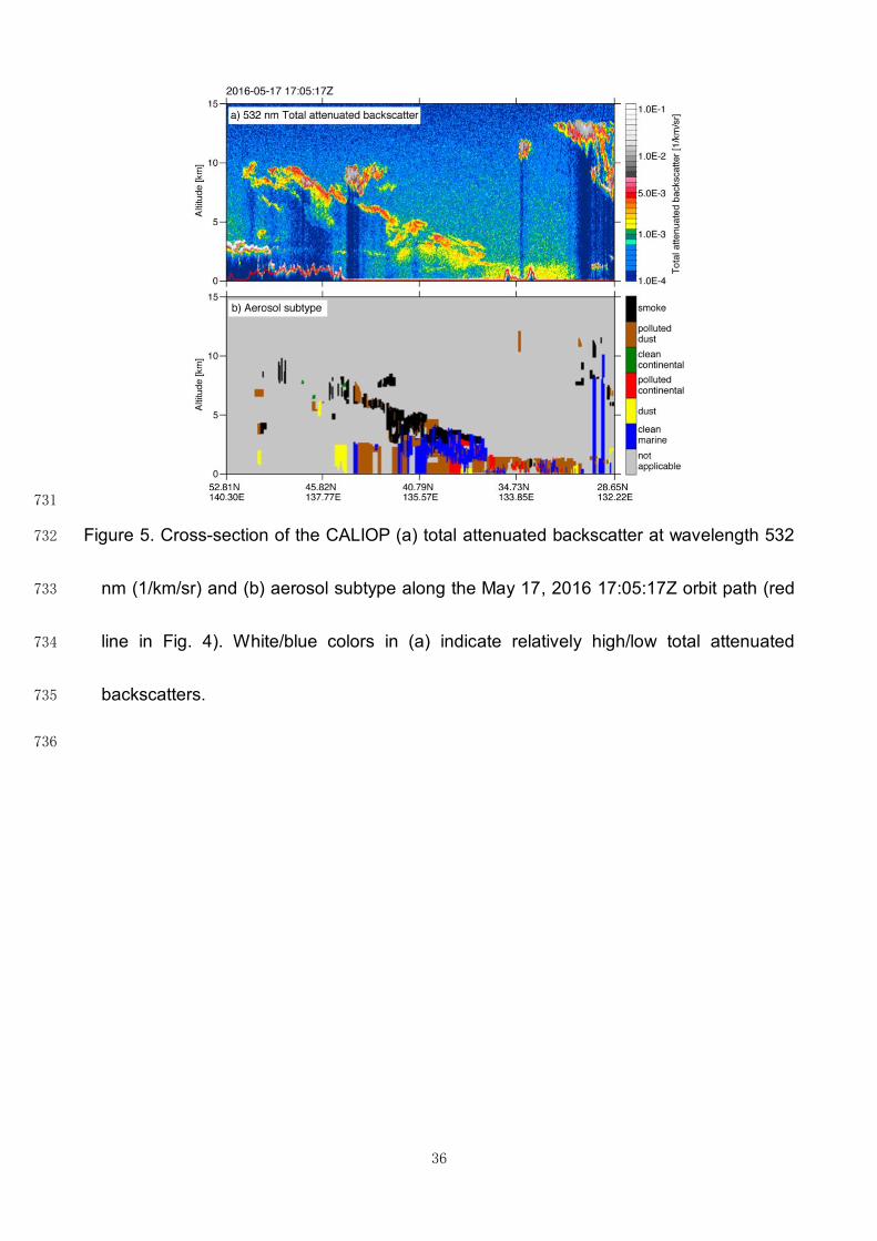
the Sea of Japan behind of a low-pressure trough. The CALIOP observations show that the 288

smoke was transported over the east coast of Siberia at an altitude of 2–8 km (Fig. 5; 289

CALIOP observation path shown in Fig. 4). Satellite observations captured the spread of the 290

smoke behind a cold front located along the Japanese archipelago on May 18, as shown in 291

the upper panels of Fig. 6. The merged AOT from Himawari-8 is consistent with AOT from 292

MODIS. The observed AOT exceeds 1.8 around the core of the smoke plume. The 293

AERONET AOT at Hokkaido_University (Fig. 7a) observed a rapid increase of AOT 294

corresponding to the motion of the smoke on May 18; the observed AOT reached 1.4, which 295

is consistent with satellite observations. 296

On the following day (May 19), the smoke covered the island of Hokkaido and the northern 297

15

part of Honshu (the main island of Japan) (Fig. 8, upper panels). The Himawari-8 AOT (Fig. 298

8a) shows a C-shaped smoke distribution. Ground-based observations also captured the 299

smoke. The AD-net Lidar at Sendai observed the dense aerosol layer at 1–5 km altitude 300

through May 19 (Fig. 9a). At Niigata, the AD-net Lidar (Fig. 9e) detected the main body of 301

the smoke; however, the extinction coefficient was lower than that of Niigata due to 302

dispersion. On May 19 and through May 20 at 0.5–4.5-km altitude (thickness: ~4 km), 303

consistent with results observed by AERONET, the Niigata AERONET showed an increase 304

in AOT due to the smoke on May 19 (Fig. 7b). 305

On May 20–21, smoke transport proceeded in two directions. The northern part of the 306

smoke traveled eastward to the northern Pacific Ocean, whereas the southern part was 307

transported from east to west across Honshu by clockwise flow associated with a high-308

pressure system centered around Hokkaido (approximately 43°N, 142°E) (Fig. 10d). This is 309

a plausible explanation for AD-net Lidar at Matsue station (in western Japan) capturing a 310

suspended smoke layer at 1–3 km on May 21 (Fig. 9i). The blue line in Fig. 4 shows the 311

backward trajectory initiated at 18:00 UTC on May 21 at Matsue at an altitude of 2 km (red 312

circle in Fig. 9i). The air mass that traveled over the source region on May 16 was 313

transported eastward over Siberia, reached Hokkaido on May 18, and was then transported 314

westward over Honshu by a clockwise flow. The arriving times of the smoke predicted by 315

the model simulation and the backward trajectory analysis are consistent with the 316

observation results. 317

16

318

4. Assimilation and forecasting results 319

Figure 6 compares the horizontal AOT distribution on May 18 between satellite 320

observations and noDA model results. Root mean square error (RMSE), linear Pearson 321

correlation coefficient (R), mean fractional error (MFE), mean fractional bias (MFB), and 322

index of agreement (IOA) calculated over the land are also shown in Fig. 6 (formulations of 323

these statistical measures are given in Appendix A). The transport of the smoke was 324

captured by the model (R and IOA are 0.66 and 0.60, respectively); however, noDA (Fig. 6d) 325

underestimated the observed AOT level and the extend of smoke in the Sea of Japan and 326

the Sea of Okhotsk (Fig. 6f). MFB of noDA is -65.6%. This underestimate persisted in the 327

noDA forecast for several days. On May 19 (Fig. 8), noDA underestimated the extent of the 328

smoke over Hokkaido and the northern part of Honshu, and did not reproduce the C-shaped 329

distribution observed by satellites (see Figs. 8d and 8g); the modeled AOTs were 0.2–0.6, 330

whereas observed AOTs exceeded 0.8, and MFB of noDA shows a large negative value (-331

73.2%). On May 20 (Fig. 10), the AOT forecast by noDA was much lower over Hokkaido and 332

the Sea of Japan than that observed by satellite (see Fig. 10g); MFB is -66.4%. Comparisons 333

between the AERONET AOT (Fig. 7) and AD-Net observations (Fig. 9) also showed that 334

noDA could forecast the advent of the smoke, but with very low AOT and extinction 335

coefficient values; the maxima of the AERONET (noDA) AOT at Hokkaido_University and 336

Niigata are 1.47 (0.51) and 0.86 (0.22), respectively. We also performed a free run with lower 337

17

spatial resolution (TL319; approximately 60 km), and found that the forecast smoke 338

distribution was quite similar between the fine and coarse models, and that the coarse model 339

also underestimated the observed AOT and extinction coefficient (data not shown). This fact 340

implies that underestimation was mainly attributed to uncertainty associated with emission 341

rather than uncertainty associated with transport (i.e., meteorological fields). Uncertainty in 342

the spatial and temporal distribution and intensity of emissions for aerosols and their 343

precursors is a major source of error in aerosol forecasting. This is particularly true for 344

aerosols from natural origins (e.g., mineral dust from desert, smoke from wildfire, and ash 345

and sulfate aerosols from volcanic eruptions); their episodic and explosive occurrences 346

make the accurate estimation of emission difficult, and result in large errors in forecasting 347

(e.g., Uno et al., 2006). In this case, the introduction of observed information in the model 348

simulation via assimilation can be effective in improving forecasting performance. 349

The analyzed AOT from DA1 at 00:00 UTC on May 18 is shown in Fig. 6e. It is clear that 350

data assimilation with Himawari-8 AOT improved the smoke distribution model. Figure 8e 351

shows a 24-h DA1 forecast (FT = 24) of AOT at 00:00 UTC on May 19 (the 24-h forecast 352

started from the analysis aerosol field at 00:00 UTC on May 18; see Fig. 1); the assimilation 353

improved the smoke forecast (all statistical measures improved comparing with noDA). 354

Specifically, the assimilation compensated for the underestimation and reproduced the C-355

shaped distribution (MFB value was reduced from -73.2% to -38.1%); however, the lower 356

bias remained in the southern part of the smoke plume (around 38–40°N, 140–150°E) and 357

18

persisted beyond the 24-h forecast (see Fig. 8h). Although the 48-h DA1 forecast (FT = 48; 358

00:00 UTC on May 20; Fig. 10e) shows better agreement and statistics with the satellite 359

observations than noDA, the forecast AOT underestimated observed AOT values (MFB is -360

45.4%). This underestimate was the result of the lower bias in the southern part of the smoke 361

plume on May 19. Although the AERONET AOT (Fig. 7) and AD-Net observation (Fig. 9) 362

confirmed the improvement in the 24–72-h forecasts due to assimilation, the DA1 forecast 363

AOT and extinction coefficient were still lower than observed values. 364

We performed a subsequent assimilation and forecasting cycle from the DA1 analysis to 365

introduce the Himawari-8 AOT May 18 observations into the forecast (Fig. 1). The results of 366

the subsequent cycle are labeled “DA2”. Figure 8f shows the analyzed AOT from DA2 at 367

00:00 UTC on May 19. Subsequent assimilation improved the modeled AOT; in particular, 368

the assimilation compensated for the underestimation in the southern part of the C-shaped 369

smoke distribution (MFB value was further reduced from -38.1% to -13.7%; compare Figs. 370

8h and 8i). Because the Himawari-8 AOTs over the land were excluded from the assimilation, 371

low AOTs over northeastern China (approximately 45°N, 132°E) in the Himawari-8 372

observation (Fig. 8a) were not reflected in the DA2 analysis and forecast. On the following 373

day (May 20; Fig. 10), the 24-h DA2 forecast (FT = 24; Figs. 10f and 10i) improved the 374

underestimation observed in the noDA forecast (Figs. 10d and 10g) and the 48-h DA1 375

forecast (Figs. 10e and 10h), and resulted in much better agreement with satellite-observed 376

AOTs. DA2 achieved better scores in all statistics than both noDA and DA1. This 377

19

improvement was verified in a comparison with AERONET observations (Fig. 7); the DA2 378

forecast quantitatively agreed with the AERONET AOT at both Hokkaido_University and 379

Niigata. The high AOT values early on May 20 at Hokkaido_University (Fig. 7a) may be 380

attributed to another smoke plume transported after the smoke examined in this study and 381

not captured by the Himawari-8 AOT used in the assimilation. This is a plausible reason for 382

the DA1 and DA2 assimilations providing a slight improvement in the high-AOT forecast. 383

Compared with AD-Net observations (Fig. 9), the DA2 forecast exhibited improvement with 384

respect to the underestimation and much better agreement with the observations than noDA 385

and DA1 forecasts. In particular, better agreement in the 48–96-h DA2 forecast at Matsue 386

on May 20–22 (Fig. 9l) indicates that the assimilation improved the forecast of the southern 387

part of the smoke plume transported across Honshu by a clockwise flow, and improved 388

performance in relatively long-term (48–96-h) forecasting. 389

The improved performance of DA2 over DA1 suggests that the inheritance of assimilation 390

cycles and the assimilation of more recent observations provides a more accurate forecast. 391

Additionally, our results imply that the benefits of the assimilation were limited to short-term 392

(i.e., 1–24-h) forecasts; this is particularly true for DA1. The DA1 assimilation run on May 17 393

improved the smoke forecast on May 18 (i.e., a 1–24-h forecast). However, in the forecasts 394

performed on the following days, the benefit of assimilation was insufficient, and the 395

concentration of the modeled smoke underestimated that of the observed smoke. We 396

excluded the Himawari-8 observations over the land from the assimilation. Therefore, the 397

20

assimilation data were obtained only around the Japanese archipelago (i.e., downwind of 398

the smoke). This is a plausible explanation for the limited benefit provided by the assimilation 399

to long-term forecasts over Japan. Including the Himawari-8 AOT observed over the land 400

(i.e., closer to the source region) in the assimilation will further improve the forecasts, 401

especially long-term forecasts. 402

We performed additional assimilation and forecasting experiments (DA1’ and DA2’) in 403

which the Himawari-8 AOTs were assimilated only at 00:00 UTC (i.e., one assimilation in 404

one assimilation run), and found little difference between DA1 and DA1’ and between DA2 405

and DA2’ (data not shown). This result implies that the most recent assimilations (in this 406

case, 00:00 UTC) had a significant impact on the forecast, and that multiple assimilations 407

(in this case, three times per day) had little effect on the forecast performance for the smoke 408

modeled in this study. One reason for this result may be the schedule of the assimilation run. 409

In DA1 and DA2, we ran the assimilations at 03:00 UTC and 06:00 UTC, took an 18-h 410

interval, ran the assimilation at 00:00 UTC, and then began the forecasts. The relatively long 411

interval between the assimilations at 06:00 UTC and 00:00 UTC increased the importance 412

of the assimilations at 00:00 UTC in these forecasts. The limitation of the ocean assimilation 413

data (i.e., the downwind region of the smoke) may provide an alternative explanation for this. 414

Utilizing the Himawari-8 AOTs over both land and ocean in the analysis will enable multiple 415

assimilations of the smoke in both the downwind and upwind regions (i.e., near the source 416

region), to further improve forecasting accuracy. 417

21

418

5. Conclusion 419

The AHI onboard Himawari-8, the 8th Japanese GMS put into operation on July 7, 2015, 420

can produce AOPs including AOT and AE, with wide vision and unprecedented temporal 421

resolution (every 10 min). In the present study, we developed an aerosol assimilation and 422

forecasting system, with which we assimilated the Himawari-8 AOT multiple times per day, 423

and performed assimilation and forecasting experiments for a heavy wildfire smoke event 424

that occurred on May 15–18, 2016 over Siberia. To take advantage of the high observational 425

frequency of the Himawari-8, we used merged AOT, which was derived from a combination 426

of 10-min AOTs, minimizing the number of pixels missing due to cloud and sunglint and 427

degradation by cloud contamination. Our results are summarized below. 428

1. The dense smoke emitted by a wildfire during May 15–18, 2016 over the eastern side 429

of Lake Baikal traveled eastward behind of a low-pressure trough, covered northern 430

Japan (Hokkaido and the northern part of the Japan main island) at an altitude of 1–5 431

km on May 19, and then branched into two parts. The northern part of the smoke was 432

transported further eastward to the northern Pacific Ocean. The southern part traveled 433

across the Japan main island in a clockwise flow associated with a high-pressure 434

system and was observed in the western part of Japan. 435

2. The free run without assimilation (noDA) forecast the observed transport of the smoke, 436

but underestimated its concentration, mainly due to errors in the emission inventory. 437

22

The data assimilation during May 17 (DA1) compensated for underestimation in the 438

forecast and reproduced the unique C-shaped distribution that noDA failed to predict. 439

However, the AOT and extinction coefficient forecast by DA1 remained lower than 440

those observed. The subsequent assimilation and forecast cycle (DA2), which 441

assimilated the Himawari-8 AOT during May 18 was greatly improved and successfully 442

predicted the transport of the smoke to the western part of Japan in its 48–96-h 443

forecast. 444

3. That DA2 performed better than DA1 in forecasting the smoke movement indicates 445

that the succeeding assimilation cycles and the assimilation of the most recent 446

observations resulted in better forecasting. Our results also implied that the 447

assimilation had an impact only on relatively short-range (i.e., 1–24-hour) forecasts of 448

the smoke in this study. The limitations of the assimilation data over the ocean (i.e., 449

data only downwind of the smoke) may be a plausible explanation for this result. 450

Further studies targeting other aerosol events than wildfire smoke (e.g., dust storms 451

and trans-boundary pollutions) and including Himawari-8 data over land are required. 452

The assimilation system has been developed for the sand and dust storm forecasting 453

operated in JMA. Our results clearly show that data assimilation with AOTs from Himawari-454

8 successfully improved the initial condition and then brought much better forecast. Although 455

this study targeted an intensive wildfire smoke case, our results indicate that AOTs from 456

Himawari-8 is promising for not only the monitoring but also improved forecasting for other 457

23

aerosol events including dust storms through data assimilation. In future studies, we will 458

perform assimilation and forecast experiments for Asian dust and storms and continental 459

anthropogenic pollutions. AOT over land (closer to continental outflow source regions) and 460

AE that are sensitive to aerosol size distribution will be utilized in assimilation during the 461

development process of these forecast models. 462

463

Appendix A: Statistical metrics 464

We used the root mean square error (RMSE), the (Pearson) correlation (R), the mean 465

fractional error (MFE), the mean fractional bias (MFB; also known as the fractional gross 466

error), and the index of agreement (IOA) for validation. The statistical metrics are defined as 467

follows: 468

RMSE = √1

𝑁∑ (𝑀𝑖 −𝑂𝑖)2𝑁𝑖=1 , (A1) 469

R =∑ (𝑂𝑖−�̅�)𝑁𝑖=1 (𝑀𝑖−�̅�)

√∑ (𝑂𝑖−�̅�)2𝑁𝑖=1 ∑ (𝑀𝑖−�̅�)2𝑁

𝑖=1

, (A2) 470

MFE =2

𝑁∑

|𝑀𝑖−𝑂𝑖|

𝑀𝑖+𝑂𝑖

𝑁𝑖=1 × 100 , (A3) 471

MFB =2

𝑁∑

𝑀𝑖−𝑂𝑖

𝑀𝑖+𝑂𝑖

𝑁𝑖=1 × 100 , (A4) 472

IOA = 1 −∑ (𝑂𝑖−𝑀𝑖)

2𝑁𝑖=1

∑ (|𝑂𝑖−�̅�|+|𝑀𝑖−�̅�|)2𝑁𝑖=1

, 473

(A5) 474

N is the total number of pairs of modeled (M) and observed (O) values. �̅� and �̅� 475

represent 1

𝑁∑ 𝑂𝑖𝑁𝑖=1 and

1

𝑁∑ 𝑀𝑖𝑁𝑖=1 , respectively. RMSE represents the standard deviation of 476

the discrepancies between modeled and observed values. MFE can range from 0 to 200%, 477

24

and is a measure of overall modeling error without emphasizing outliers. MFE = 0 is a perfect 478

score. MFB is a measure of the estimation bias error that allows symmetric analysis of over- 479

or underestimation by the model relative to observed values. The best value of MFB is 0 480

with ±200% the minimum and maximum values. Boylan and Russell (2006) proposed that 481

MFE should be ≤ +50% and MFB should be ≤ ±30% to meet model performance goals for 482

particulate matter (PM) and light extinction. IOA was developed by Willmott (1981) as a 483

standard measure of the degree of model prediction accuracy, and it ranges from 0 to 1. IOA 484

= 1 indicates perfect agreement. 485

486

Acknowledgments 487

This work was supported by the Japan Society for the Promotion of Science (JSPS) 488

KAKENHI, Grant Numbers JP25220101, JP15K05296, and JP16H02946, and by the 489

Environment Research and Technology Development Fund (No. S-12) of the Japanese 490

Ministry of Environment. We thank all of the principal investigators and those who 491

contributed to the establishment and maintenance of the Himawari-8 AOPs, the AERONET 492

sites, CALIOP/CALIPSO, the NOAA HYSPLIT trajectory model, and the NASA MODIS L2 493

aerosol products. 494

495

References 496

Benedetti, A., J.-J. Morcrette, O. Boucher, A. Dethof, R.J. Engelen, M. Fisher, H. Flentje, 497

N. Huneeus, L. Jones, J.W. Kaiser, S. Kinne, A. Mangold, M. Razinger, A.J. 498

25

Simmons, and M. Suttie, 2009: Aerosol analysis and forecast in the European Centre 499

for Medium-Range Weather Forecasts Integrated Forecast System: 2. Data 500

assimilation. J. Geophys. Res., 114, D13205, doi:10.1029/2008JD011115. 501

Bessho, K., K. Date, M. Hayashi, A. Ikeda, T. Imai, H. Inoue, Y. Kumaga, T. Miyakawa, H. 502

Murata, T. Ohno, A. Okuyama, R. Oyama, Y. Sasaki, Y. Shimazu, K. Shimoji, Y. 503

Sumida, M. Suzuki, H. Taniguchi, H. Tsuchiyama, D. Uesawa, H. Yokota, and R. 504

Yoshida, 2016: An introduction to Himawari-8/9 - Japan’s new-generation 505

geostationary meteorological satellites. J. Meteorol. Soc. Japan, 94, 151–183, 506

doi:10.2151/jmsj.2016-009. 507

Boylan, J. W. and A. G. Russell, 2006: PM and light extinction model performance metrics, 508

goals, and criteria for three-dimensional air quality models, Atmos. Environ., 40, 509

4946–4959, doi:10.1016/j.atmosenv.2005.09.087, 2006. 510

Daley, R., and E. Barker, 2001: NAVDAS: formulation and diagnostics. Mon. Weather 511

Rev., 129, 869–883, doi:10.1175/1520-0493(2001)129<0869:NFAD>2.0.CO;2. 512

Gong, S. L., 2003: A parameterization of sea-salt aerosol source function for sub- and 513

super-micron particles. Global Biogeochem. Cycles, 17, 1–7, 514

doi:10.1029/2003GB002079. 515

Grell, G., and A. Baklanov, 2011: Integrated modeling for forecasting weather and air 516

quality: a call for fully coupled approaches. Atmos. Environ., 45, 6845–6851, 517

doi:10.1016/j.atmosenv.2011.01.017. 518

Grell, G., S.R. Freitas, M. Stuefer, and J. Fast, 2011: Inclusion of biomass burning in 519

WRF-Chem: impact of wildfires on weather forecasts. Atmos. Chem. Phys., 11, 5289–520

5303, doi:10.5194/acp-11-5289-2011. 521

Holben, B.N., T.F. Eck, I. Slutsker, D. Tanre, J.P. Buis, A. Setzer, E. Vermote, J.A. 522

Reagan, Y.J. Kaufman, T. Nakajima, F. Lavenu, I. Jankowiak, and A. Smirnov, 1998: 523

AERONET - a federated instrument network and data archive for aerosol 524

characterization. Remote Sens. Environ., 66, 1–16. 525

Hunt, B., E. Kostelich, and I. Szunyogh, 2007: Efficient data assimilation for spatiotemporal 526

chaos: a local ensemble transform Kalman filter. Phys. D Nonlinear Phenom., 230, 527

112–126, doi:10.1016/j.physd.2006.11.008. 528

IPCC, 2013: Climate Change 2013: The Physical Science Basis. Contribution of Working 529

Group I to the Fifth Assessment Report of the Intergovernmental Panel on Climate 530

Change, eds.: Stocker, T. F., D. Qin, G.-K. Plattner, M. Tignor, S.K. Allen, J. 531

Boschung, A. Nauels, Y. Xia, V. Bex, and P.M. Midgley, Cambridge University Press, 532

Cambridge, UK. 533

JMA, 2002: Annual WWW Technical Progress Report on the Global Data Processing 534

System: Japan Meteorological Agency. GDPS Technical Progress Report Series No. 535

12, WMO/TD-No. 1148-21.03.03. Japan Meteorological Agency, Tokyo, Japan. 536

Kikuchi, M., T.M. Nagao, and H. Murakami, 2017: Development of Hourly Combined Aerosol 537

Optical Thickness Algorithm from Himawari-8, IEEE Trans. Geosci. Remote Sens., 538

26

2018, in print. 539

Levy, R.C., S. Mattoo, L.A. Munchak, L.A. Remer, A.M. Sayer, F. Patadia, and N.C. Hsu, 540

2013: The Collection 6 MODIS aerosol products over land and ocean. Atmos. Meas. 541

Tech., 6, 2989–3034, doi:10.5194/amt-6-2989-2013. 542

Levy, R., and C. Hsu, 2015: MODIS Atmosphere L2 Aerosol Product, NASA MODIS 543

Adaptive Processing System, Goddard Space Flight Center, USA, 544

doi:10.5067/MODIS/MOD04_L2.006. 545

Morcrette, J.J., A. Benedetti, A. Ghelli, J. Kaiser, and A. Tompkins, 2011: Aerosol–Cloud–546

Radiation Interactions and their Impact on ECMWF/MACC Forecasts. ECMWF 547

Technical Memorandum 660. 548

Mulcahy, J.P., D.N. Walters, N. Bellouin, and S.F. Milton, 2014: Impacts of increasing the 549

aerosol complexity in the Met Office global numerical weather prediction model. 550

Atmos. Chem. Phys., 14, 4749–4778, doi:10.5194/acp-14-4749-2014. 551

Parrish, D.F., and J.C. Derber, 1992: The National Meteorological Center’s Spectral 552

Statistical-Interpolation Analysis System. Mon. Weather Rev., 120, 1747–1763, 553

doi:10.1175/1520-0493(1992)120<1747:TNMCSS>2.0.CO;2. 554

Pérez, C., S. Nickovic, G. Pejanovic, J.M. Baldasano, and E. Özsoy, 2006: Interactive 555

dust-radiation modeling: a step to improve weather forecasts. J. Geophys. Res., 111, 556

D16206, doi:10.1029/2005JD006717. 557

Rodwell, M.J., and T. Jung, 2008: Understanding the local and global impacts of model 558

physics changes: an aerosol example. Q. J. R. Meteorol. Soc., 134, 1479–1497, 559

doi:10.1002/qj.298. 560

Rubin, J.I., J.S. Reid, J.A. Hansen, J.L. Anderson, N. Collins, T.J. Hoar, T. Hogan, P. 561

Lynch, J. McLay, C.A. Reynolds, W.R. Sessions, D.L. West, and J. Zhang, 2016: 562

Development of the Ensemble Navy Aerosol Analysis Prediction System (ENAAPS) 563

and its application of the Data Assimilation Research Testbed (DART) in support of 564

aerosol forecasting. Atmos. Chem. Phys., 16, 3927–3951, doi:10.5194/acp-16-3927-565

2016. 566

Rubin, J.I., J.S. Reid, J.A. Hansen, J.L. Anderson, B.N. Holben, P. Lynch, D.L. Westphal, 567

and J. Zhang, 2017: Assimilation of AERONET and MODIS AOT observations using 568

variational and ensemble data assimilation methods and its impact on aerosol 569

forecasting skill. J. Geophys. Res. Atmos., doi:10.1002/2016JD026067. 570

Sessions, W.R., J.S. Reid, A. Benedetti, P.R. Colarco, A. de Silva, S. Lu, T. Sekiyama, 571

T.Y. Tanaka, J.M. Baldasano, S. Basart, M.E. Brooks, T.F. Eck, M. Iredell, J.A. 572

Hansen, O.C. Jorba, H.-M.H. Juang, P. Lynch, J.-J. Morcrette, S. Moorthi, J. Mulcahy, 573

Y. Pradhan, M. Razinger, C.B. Sampson, J. Wang, and D.L. Westphal, 2015: 574

Development towards a global operational aerosol consensus: basic climatological 575

characteristics of the International Cooperative for Aerosol Prediction Multi-Model 576

Ensemble (ICAP-MME). Atmos. Chem. Phys., 15, 335–362, doi:10.5194/acp-15-335-577

2015. 578

27

Shao, Y., M. Raupach, and J. Leys, 1996: A model for predicting aeolian sand drift and 579

dust entrainment on scales from paddock to region. Aust. J. Soil Res., 34, 309, 580

doi:10.1071/SR9960309. 581

Stein, A.F., R.R. Draxler, G.D. Rolph, B.J.B. Stunder, M.D. Cohen, and F. Ngan, 2015: 582

NOAA’s HYSPLIT atmospheric transport and dispersion modeling system. Bull. Am. 583

Meteorol. Soc., 96, 2059–2077, doi:10.1175/BAMS-D-14-00110.1. 584

Sugimoto, N., I. Matsui, A. Shimizu, T. Nishizawa, Y. Hara, and I. Uno, 2008: Lidar 585

network observations of tropospheric aerosols. Proc. SPIE, 7153, 71530A–71530A–586

13, doi:10.1117/12.806540. 587

Tanaka, T.Y., and M. Chiba, 2005: Global simulation of dust aerosol with a chemical 588

transport model, MASINGAR. J. Meteorol. Soc. Japan, 83A, 255–278, 589

doi:10.2151/jmsj.83A.255. 590

Terradellas, E., S. Nickovic, and X. Zhang, 2015: Airborne dust: a hazard to human health, 591

environment and society, WMO Bull., 64, 42–46. 592

Toll, V., E. Gleeson, K.P. Nielsen, A. Männik, J. Mašek, L. Rontu, and P. Post, 2016: 593

Impacts of the direct radiative effect of aerosols in numerical weather prediction over 594

Europe using the ALADIN-HIRLAM NWP system. Atmos. Res., 172–173, 163–173, 595

doi:10.1016/j.atmosres.2016.01.003. 596

Di Tomaso, E., N.A.J. Schutgens, O. Jorba, and C. Pérez García-Pando, 2016: 597

Assimilation of MODIS Dark Target and Deep Blue observations in the dust aerosol 598

component of NMMB/BSC-CTM version 1.0. Geosci. Model Dev. Discuss., 10, 1–35, 599

doi:10.5194/gmd-2016-206. 600

Uno, I., and Z. Wang, M. Chiba,Y. S. Chun, S. L. Gong, Y. Hara, E. Jung, S.-S. Lee, M. 601

Liu, M. Mikami, S. Music, S. Nickovic, S. Satake, Y. Shao, Z. Song, N. Sugimoto, T. 602

Tanaka, and D. L. Westphal, 2006: Dust model intercomparison (DMIP) study over 603

Asia: Overview. J. Geophys. Res., 111, doi:10.1029/2005JD006575. 604

Wang, H., and T. Niu, 2013: Sensitivity studies of aerosol data assimilation and direct 605

radiative feedbacks in modeling dust aerosols. Atmos. Environ., 64, 208–218, 606

doi:10.1016/j.atmosenv.2012.09.066. 607

WHO, 2016: Ambient air pollution: A global assessment of exposure and burden of 608

disease. The WHO Document Production Services, Geneva, Switzerland, 2016. 609

(http://apps.who.int/iris/bisream/10665/250141/1/978241511353-eng.pdf). 610

Willmott, C. J., 1981: On the validation of models, Phys. Geogr., 2, 184–194, 611

doi:10.1080/02723646.1981.10642213. 612

Winker, D.M., J. Pelon, J.A. Coakley, S.A. Ackerman, R.J. Charlson, P.R. Colarco, P. 613

Flamant, Q. Fu, R.M. Hoff, C. Kittakam T.L. Kubar, H. Le Treut, M.P. McCormick, G. 614

Megie, L. Poole, K. Powell, C. Trepte, M.A. Vaughan, and B.A. Wielicki, 2010: The 615

CALIPSO Mission: A Global 3D View of Aerosols and Clouds. Bull. Am. Meteorol. 616

Soc., 91, 1211–1229, doi:10.1175/2010BAMS3009.1. 617

Yoshida, M., M. Kikuchi, T.M. Nagao, and H. Murakami: Approach to commonly retrieve 618

28

the aerosol optical properties for various imaging satellite sensor, J. Meteorol. Soc. 619

Japan, submitted. 620

Yukimoto, S., Y. Adachi, M. Hosaka, T. Sakami, H. Yoshimura, M. Hirabara, T.Y. Tanaka, 621

E. Shindo, H. Tsujino, M. Deushi, R. Mizuta, S. Yabu, A. Obata, H. Nakano, T. 622

Koshiro, T. Ose, and A. Kitoh, 2012: A new global climate model of the Meteorological 623

Research Institute: MRI-CGCM3 – model description and basic performance, J. 624

Meteorol. Soc. Japan, 90A, 23–64, doi:10.2151/jmsj.2012-A02. 625

Yumimoto, K., T.M. Nagao, M. Kikuchi, T.T. Sekiyama, H. Murakami, T.Y. Tanaka, A. Ogi, 626

H. Irie, P. Khatri, H. Okumura, K. Arai, I. Morino, O. Uchino, and T. Maki, 2016a: 627

Aerosol data assimilation using data from Himawari-8, a next-generation 628

geostationary meteorological satellite. Geophys. Res. Lett., 43, 5886–5894, 629

doi:10.1002/2016GL069298. 630

Yumimoto, K., H. Murakami, T.Y. Tanaka, T.T. Sekiyama, A. Ogi, and T. Maki, 2016b: 631

Forecasting of Asian dust storm that occurred on May 10–13, 2011, using an 632

ensemble-based data assimilation system. Particuology, 28, 121–130, 633

doi:10.1016/j.partic.2015.09.001. 634

Yumimoto, K., T.Y. Tanaka, N. Oshima, and T. Maki, 2017: JRAero: the Japanese 635

reanalysis for Aerosol v1.0. Geosci. Model Dev. Discuss., 1–52, doi:10.5194/gmd-636

2017-72. 637

Zhang, J., J.S. Reid, D.L. Westphal, N.L. Baker, and E.J. Hyer, 2008: A system for 638

operational aerosol optical depth data assimilation over global oceans. J. Geophys. 639

Res., 113, 1–13, doi:10.1029/2007JD009065. 640

641

642

643

644

List of Figures 645

Figure 1. Schematic diagram of the assimilation and forecasting experiment. 646

647

Figure 2. Horizontal distributions of (a and d) first-guess aerosol optical thickness, (b and e) 648

variance, and (c and f) covariance of the grid situated at 45.14°N, 136.13°E and 42.89°N, 649

and 141.00°E, respectively. Red circles show distances from the grids. Upper panels are 650

29

for 00:00 UTC on May 18, 2016; lower panels are for 00:00 UTC on May 19, 2016. 651

Red/blue colors in left and central panels indicate relatively high/low AOTs and variances, 652

respectively. Red/gray colors in right panels indicate positive/negative covariances. 653

654

Figure 3. Horizontal distribution of aerosol optical thickness (AOT) retrieved from Himawari-655

8 data at 03:00 UTC on May 18, 2016. (a) AOT from the L2 product; (b) merged AOT from 656

the L3 product; (c) uncertainty from the L2 product. Red/blue colors indicate relatively 657

high/low AOTs. 658

659

Figure 4. Horizontal distribution of wildfire flux of organic carbon (g/m2/day) on May 16, 2016. 660

Red/green colors indicate relatively high/low wildfire fluxes. Red dots denote Himawari-8 661

wildfire detection. AD-Net Lidar and AERONET stations are indicated by magenta squares 662

and orange triangles, respectively. Red lines indicate the CALIPSO orbit path. The blue 663

line denotes the HYSPLIT backward trajectory started at 18:00 UTC on May 21 at 2,000 664

m above Matsue. 665

666

Figure 5. Cross-section of the CALIOP (a) total attenuated backscatter at wavelength 532 667

nm (1/km/sr) and (b) aerosol subtype along the May 17, 2016 17:05:17Z orbit path (red 668

line in Fig. 4). White/blue colors in (a) indicate relatively high/low total attenuated 669

backscatters. 670

30

671

Figure 6. Horizontal distribution of observed and modeled AOT on May 18, 2016: (a) 672

observed from Himawari-8, (b) observed from MODIS/Terra, (c) observed from 673

MODIS/Aqua, (d) modeled from noDA run, (e) modeled from DA1 run, (f) difference 674

between Himawari-8 and noDA run, and (g) difference between Himawari-8 and DA1 run. 675

RMSE, correlation coefficient (R), IOA, MFB, and MFE values are also shown. Red/blue 676

colors in upper and middle panels indicate relatively high/low AOTs. Red/blue colors in 677

lower panels indicate positive/negative values of difference of AOT. 678

679

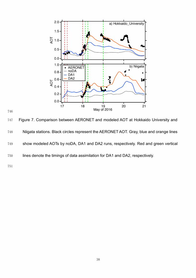
Figure 7. Comparison between AERONET and modeled AOT at Hokkaido_University and 680

Niigata stations. Black circles represent the AERONET AOT. Gray, blue and orange lines 681

show modeled AOTs by noDA, DA1 and DA2 runs, respectively. Red and green vertical 682

lines denote the timings of data assimilation for DA1 and DA2, respectively. 683

684



MODIS/Aqua, (d) modeled from noDA run, (e) modeled from the DA1 run, (f) modeled 687

AOT from the DA2 run, (g) difference between Himawari-8 and noDA run, and (h) 688

difference between Himawari-8 and DA1 run, and (i) difference between Himawari-8 and 689

DA2 run. RMSE, correlation coefficient (R), IOA, MFB, and MFE values are also shown. 690

31

Red/blue colors in upper and middle panels indicate relatively high/low AOTs. Red/blue 691

colors in lower panels indicate positive/negative values of difference of AOT. 692

693

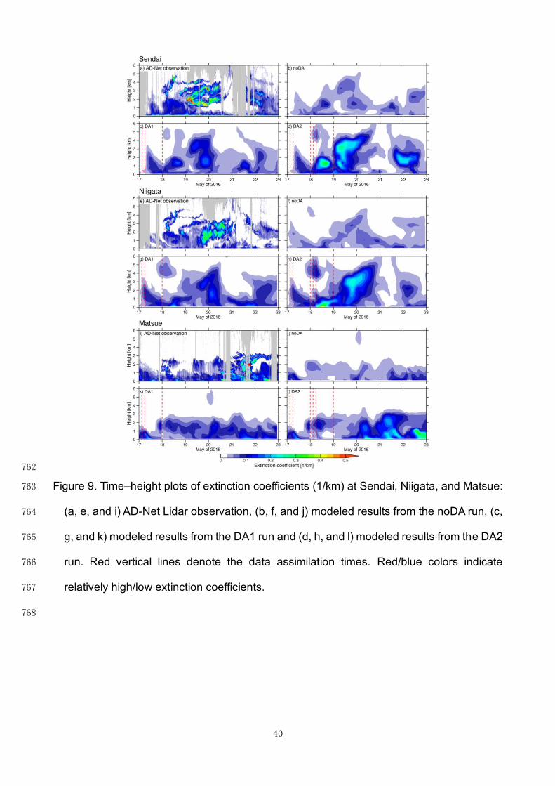
Figure 9. Time–height plots of extinction coefficients (1/km) at Sendai, Niigata, and Matsue: 694

(a, e, and i) AD-Net Lidar observation, (b, f, and j) modeled results from the noDA run, (c, 695

g, and k) modeled results from the DA1 run and (d, h, and l) modeled results from the DA2 696

run. Red vertical lines denote the data assimilation times. Red/blue colors indicate 697

relatively high/low extinction coefficients. 698

699

Figure 10. As for Fig. 8, but for May 20, 2016. 700

701

702

32

703

Figure 1. Schematic diagram of the assimilation and forecasting experiment. Black circles 704

denote the data assimilation times. 705

706

707

33

708

Figure 2. Horizontal distributions of (a and d) first-guess aerosol optical thickness, (b and e) 709

variance, and (c and f) covariance of the grid situated at 45.14°N, 136.13°E and 42.89°N, 710

and 141.00°E, respectively. Red circles show distances from the grids. Upper panels are 711

for 00:00 UTC on May 18, 2016; lower panels are for 00:00 UTC on May 19, 2016. 712

Red/blue colors in left and central panels indicate relatively high/low AOTs and variances, 713

respectively. Red/gray colors in right panels indicate positive/negative covariances. 714

715

716

34

717

Figure 3. Horizontal distribution of aerosol optical thickness (AOT) retrieved from Himawari-718

8 data at 03:00 UTC on May 18, 2016. (a) AOT from the L2 product; (b) merged AOT from 719

the L3 product; (c) uncertainty from the L2 product. Red/blue colors indicate relatively 720

high/low AOTs. 721

722

35

723

Figure 4. Horizontal distribution of wildfire flux of organic carbon (g/m2/day) on May 16, 2016. 724

Red/green colors indicate relatively high/low wildfire fluxes. Red dots denote Himawari-8 725

wildfire detection. AD-Net Lidar and AERONET stations are indicated by magenta squares 726

and orange triangles, respectively. Red lines indicate the CALIPSO orbit path. The blue 727

line denotes the HYSPLIT backward trajectory started at 18:00 UTC on May 21 at 2,000 728

m above Matsue. 729

730

36

731

Figure 5. Cross-section of the CALIOP (a) total attenuated backscatter at wavelength 532 732

nm (1/km/sr) and (b) aerosol subtype along the May 17, 2016 17:05:17Z orbit path (red 733

line in Fig. 4). White/blue colors in (a) indicate relatively high/low total attenuated 734

backscatters. 735

736

37

737



MODIS/Aqua, (d) modeled from noDA run, (e) modeled from DA1 run, (f) difference 740

between Himawari-8 and noDA run, and (g) difference between Himawari-8 and DA1 run. 741

Red broken lines show modeled sea level pressure with the locations of low and high 742

pressure systems. RMSE, correlation coefficient (R), IOA, MFB, and MFE values are also 743

shown. Red/blue colors in upper and middle panels indicate relatively high/low AOTs. 744

Red/blue colors in lower panels indicate positive/negative values of difference of AOT. 745

38

746

Figure 7. Comparison between AERONET and modeled AOT at Hokkaido University and 747

Niigata stations. Black circles represent the AERONET AOT. Gray, blue and orange lines 748

show modeled AOTs by noDA, DA1 and DA2 runs, respectively. Red and green vertical 749

lines denote the timings of data assimilation for DA1 and DA2, respectively. 750

751

39

752



MODIS/Aqua, (d) modeled from noDA run, (e) modeled from the DA1 run, (f) modeled 755

AOT from the DA2 run, (g) difference between Himawari-8 and noDA run, and (h) 756

difference between Himawari-8 and DA1 run, and (i) difference between Himawari-8 and 757

DA2 run. Red broken lines show modeled sea level pressure with the locations of low and 758

high pressure systems. RMSE, correlation coefficient (R), IOA, MFB, and MFE values are 759

also shown. Red/blue colors in upper and middle panels indicate relatively high/low AOTs. 760

Red/blue colors in lower panels indicate positive/negative values of difference of AOT. 761

40

762

Figure 9. Time–height plots of extinction coefficients (1/km) at Sendai, Niigata, and Matsue: 763

(a, e, and i) AD-Net Lidar observation, (b, f, and j) modeled results from the noDA run, (c, 764

g, and k) modeled results from the DA1 run and (d, h, and l) modeled results from the DA2 765

run. Red vertical lines denote the data assimilation times. Red/blue colors indicate 766

relatively high/low extinction coefficients. 767

768

41

769

Figure 10. As for Fig. 8, but for May 20, 2016. 770

771

772

EARLY ONLINE RELEASE - JST

Documents

Transcript of EARLY ONLINE RELEASE - JST