Early estimates of euro area real GDP growth: a bottom up approach ...

Work ing PaPer Ser i e Sno 975 / December 2008

earLY eSTimaTeS oF eUro area reaL gDP groWTH

a boTTom UP aPProacH From THe ProDUcTion SiDe

by Elke Hahn and Frauke Skudelny

WORKING PAPER SER IESNO 975 / DECEMBER 2008

In 2008 all ECB publications

feature a motif taken from the

10 banknote.

EARLY ESTIMATES OF EURO AREA

REAL GDP GROWTH

A BOTTOM UP APPROACH FROM

THE PRODUCTION SIDE 1

by Elke Hahn 2 and Frauke Skudelny 2

This paper can be downloaded without charge fromhttp://www.ecb.europa.eu or from the Social Science Research Network

electronic library at http://ssrn.com/abstract_id=1304533.

1 The views expressed in this paper are those of the authors and do not necessarily reflect those of the European Central Bank.

We are grateful for comments from an anonymous referee, Domenico Giannone, Neale Kennedy, Vincent Labhard,

Michele Lenza, David Lodge, Julian Morgan, Philip Vermeulen and other participants at an internal ECB seminar

and at the 28th International Symposium on Forecasting (ISF), 2008.

2 European Central Bank, Kaiserstrasse 29, D - 60311 Frankfurt am Main, Germany:

email: [email protected], [email protected].

© European Central Bank, 2008

Address Kaiserstrasse 29 60311 Frankfurt am Main, Germany

Postal address Postfach 16 03 19 60066 Frankfurt am Main, Germany

Telephone +49 69 1344 0

Website http://www.ecb.europa.eu

Fax +49 69 1344 6000

All rights reserved.

Any reproduction, publication and reprint in the form of a different publication, whether printed or produced electronically, in whole or in part, is permitted only with the explicit written authorisation of the ECB or the author(s).

The views expressed in this paper do not necessarily refl ect those of the European Central Bank.

The statement of purpose for the ECB Working Paper Series is available from the ECB website, http://www.ecb.europa.eu/pub/scientific/wps/date/html/index.en.html

ISSN 1561-0810 (print) ISSN 1725-2806 (online)

3ECB

Working Paper Series No 975December 2008

Abstract 4

Non-technical summary 5

1 Introduction 7

2 Methodology 9

2.1 Pre-selection of the set of monthly variables 10

2.2 Set up of the pool of bridge equations 12

2.3 Framework of forecast competition and evaluation 13

2.4 Treatment of remaining components and aggregation to GDP forecast 18

3 Empirical results 18

3.1 Variables selected in the best equations 18

3.2 Forecast performance of bridge equations 20

3.3 Forecast performance of the other components and GDP 24

3.4 Comparison of fi tted values and outcomes 24

4 Conclusions 25

References 28

Appendices 29

European Central Bank Working Paper Series 61

CONTENTS

4ECBWorking Paper Series No 975December 2008

Abstract

This paper derives forecasts for euro area real GDP growth based on a bottom up approach from the production side. That is, GDP is forecast via the forecasts of value added across the different branches of activity, which is quite new in the literature. Linear regression models in the form of bridge equations are applied. In these models earlier available monthly indicators are used to bridge the gap of missing GDP data. The process of selecting the best performing equations is accomplished as a pseudo real time fore-casting exercise, i.e. due account is taken of the pattern of available monthly variables over the forecast cycle. Moreover, by applying a very systematic procedure the best performing equations are selected from a pool of thousands of test bridge equations. Our modelling approach, finally, includes a further novelty which should be of particular interest to practitioners. In practice, forecasts for a particular quarter of GDP generally spread over a prolonged period of several months. We explore whether over this forecast cycle, where GDP is repeatedly forecast, the same set of equations or different ones should be used. Changing the set of bridge equations over the forecast cycle could be superior to keeping the same set of equations, as the relative merit of the included monthly indictors may shift over time owing to differences in their data characteristics. Overall, the models derived in this forecast exercise clearly outperform the benchmark models. The variables selected in the best equations for different situations over the forecast cycle vary substantially and the achieved results confirm the conjecture that allowing the variables in the bridge equations to differ over the forecast cycle can lead to substantial improvements in the forecast accuracy.

Keywords: Forecasting, bridge equations, euro area, GDP, bottom up approach

JEL classification: C22, C52, C53, E27

5ECB


Non‐technical summary

Early information on the state of the economy is at the essence, in particular, for policy

makers. Conjunctural analysis, however, is hampered by the publication delays of important

official statistics such as those of national accounts. Meanwhile, the assessment of the state of

the economy has to be based on more timely available monthly conjunctural indicators. In

this connection, short‐term forecasting models have proved a convenient way of combining

and filtering the multitude of signals derived from the large number of relevant monthly

indicators into an encompassing joint view on the prospects of GDP growth.

Different types of forecasting models have been applied in the literature to take up this

challenge. These include, in particular, linear regression models and factor models. Apart

from the type of models, a further distinguishing feature in forecasting GDP relates to the

level of disaggregation at which the forecast is conducted. Most analyses focus on forecasting

GDP directly at the aggregate level, but there may be benefits in forecasting GDP more

indirectly via its sub‐components. Such forecasts could outperform direct GDP forecasts as

the included explanatory variables may be more tailor‐made for predicting particular sub‐

components of GDP than the aggregate. Moreover, a forecast at disaggregate level contains

the advantage of also providing background information on the drivers of the outcome of

the GDP forecast. Baffigli, Golinelli and Parigi (2002) have taken up the disaggregated

approach providing forecasts for GDP from the demand side via its expenditure

components.

The current paper presents a new forecasting framework for euro area GDP based on its sub‐

components, where, different to Baffigli et al (2002), GDP is not forecast via the demand side

but from the supply side of the economy. This can be seen as a complement to the demand

side approach. But given the larger amount of specific conjunctural indicators for branches of

activity compared with those for expenditure components, it could also turn out that the

supply side approach outperforms the demand side forecast. The applied forecast

framework is based on linear regression models. These models are used in the form of so

called bridge equations. The name bridge equations reflects the idea of using earlier available

monthly indicators to bridge the gap of missing GDP data. In order to mimic as close as

possible the true forecast situation, these GDP forecasts are derived in two steps. In a first

step, missing data points of the monthly indicators for some or all of the months of the


quarter of interest are forecast with time series models. In a second step, quarterly GDP

growth is predicted based on the quarterly aggregates of the already available and

(otherwise) predicted monthly variables. A further specialty of our approach is the effort we

put in finding the best performing bridge equations. By applying a very systematic

procedure, we select the best equations among thousands of test bridge equations. Our

modelling approach, finally, includes a novelty which should be of particular interest for

practitioners. In practice, forecasts for a particular quarter of GDP generally spread over a

prolonged period of several months. We explore whether over this forecast cycle, where

GDP is repeatedly forecast, the same set of bridge equations or different ones should be

used. Changing the set of bridge equations over the forecast cycle could be superior to

keeping the same set of equations, as the relative merit of the different included monthly

indictors may shift over time owing to differences in their data characteristics.

The results show that all models selected in this forecast exercise clearly outperform the

benchmark models. The variables included in the best equations, that are specifically selected

to forecast value added at particular stages over the forecast cycle, vary substantially over

the cycle pointing to clear changes in the relative importance of individual variables over

time. A general observation is, for instance, that survey information appears of particular

value at the early stages of the forecast cycle, while hard data, such as industrial production,

which are quite volatile but show a high degree of co movement with quarterly value added

growth, are very important only at the latest stages of the forecast cycle. In line with this, it

clearly turns out that the forecast accuracy is higher for the equations that are more

specifically selected to forecast GDP at particular stages over the forecast cycle compared to

the equations that are kept unchanged over the whole cycle. This confirms the conjecture that

changing the set of equations over the forecast cycle is superior to keeping the same

equations over time. Comparing the forecast performance of the bridge equations across

branches of activity, it turns out that the magnitude of the RMSEs varies substantially across

sectors. Probably related to differences in the volatility of the data, the RMSEs are much

higher in the construction and industrial sectors than in the services sectors. At the same

time, however, the improvement in forecast accuracy over the cycle is smaller in services

than in industry and construction, which most likely reflects the scarcity and quality of

monthly hard data in services compared to industry and construction.

7ECB


1. Introduction

Early information on the state of the economy is at the essence, in particular, for policy

makers. Conjunctural analysis, however, is hampered by the publication delays of important

official statistics such as those of national accounts. In the euro area, a flash estimate of GDP

is released only one and a half months following the reference quarter and a first full release

of national accounts, which also includes information on the breakdown of GDP by

expenditure components and branches of activity, becomes available only two months after

the end of the reference quarter. Meanwhile, the assessment of the state of the economy has

to be based on more timely available monthly conjunctural indicators. In this connection,

short term forecasting models have proved a convenient way of combining and filtering the

multitude of signals derived from the large number of relevant monthly indicators into an

encompassing joint view on the prospects of GDP growth.1

Different types of forecasting models have been applied in the literature to take up this

challenge. These include, in particular, linear regression models and factor models. The

former class of models can probably be described as the most frequently used ones (for

examples see e.g. Rünstler and Sédillot (2003) and Diron (2008)), but more recently the latter

type of models has gained increasing popularity as well (see e.g. Angelini, Camba Mendez,

Giannone, Reichlin and Rünstler (2008), Giannone, Reichlin and Small (2006) and Altissimo,

Cristadoro, Forni, Lippi and Veronese (2007)). Apart from the type of models, a further

distinguishing feature in forecasting GDP relates to the level of disaggregation at which the

forecast is conducted. Most analyses focus on forecasting GDP directly at the aggregate level,

but there may be benefits in forecasting GDP more indirectly via its sub components. Such

forecasts could outperform direct GDP forecasts as the included explanatory variables may

be more tailor made for predicting particular sub components of GDP than the aggregate.

Moreover, a forecast at disaggregate level contains the advantage of also providing

background information on the drivers of the outcome of the GDP forecast. Baffigli, Golinelli

and Parigi (2002) have taken up the disaggregated approach. Besides providing a direct

1 See also ECB (2008).


forecast for aggregate GDP, they also forecast GDP from the demand side via its expenditure

components.

The current paper presents a new forecasting framework for euro area GDP based on linear

regression models for its sub components. Different to Baffigli et al (2002) but in line with

Angelini, Banbura and Rünstler (2008), GDP is not forecast via the demand side but from the

supply side of the economy. Taking the production perspective can be seen as a complement

to the demand side approach. The benefits of applying both approaches include the

possibility of accomplishing a more encompassing analysis of the sources of a particular

outcome of GDP. It can for example be analysed whether GDP growth may be weak due to

subdued growth in a specific expenditure component, or whether this may result from

structural problems or shocks to a particular economic sector. Moreover, running both

approaches contemporaneously not only helps to detect the stories behind the outcome of

the forecast, but may likewise serve cross checking purposes. Given the known

interconnections and significant overlaps between demand and supply side components of

GDP (such as e.g. in the case of the euro area between private consumption on the one side

and the services sector on the other side) applying both approaches helps to examine the

plausibility of the results and to detect inconsistencies, in particular, in case of forecast

deviations. With this information in mind, it may also be easier to draw conclusions on the

relative trustworthiness of the deviating forecasts at that stage. More generally, given the

larger amount of specific conjunctural indicators for branches of activity compared with

those for expenditure components, it could also turn out that the supply side approach

outperforms the demand side forecast.

As already indicated above, the modelling strategy followed in this paper is based on linear

regression models. These models are applied in the form of so called bridge equations (see

Parigi and Schlitzer (1995)). The name bridge equations reflects the idea of using earlier

available monthly indicators to bridge the gap of missing GDP data. In order to mimic as

close as possible the true forecast situation, these GDP forecasts are derived in two steps. In a

first step, missing data points of the monthly indicators for some or all of the months of the

quarter of interest are forecast with time series models. In a second step, quarterly GDP

growth is predicted based on the quarterly aggregates of the already available and

(otherwise) predicted monthly variables. A further specialty of our approach is the effort we

9ECB


put in finding the best performing bridge equations. By applying a very systematic

procedure, we select the best equations among thousands of test bridge equations. Our

modelling approach, finally, includes a novelty which should be of particular interest for

practitioners. In practice, forecasts for a particular quarter of GDP generally spread over a

prolonged period of several months. We explore whether over this forecast cycle the same

set of bridge equations or different ones should be used to forecast GDP. Changing the set of

bridge equations over the forecast cycle could be superior to keeping the same set of

equations, as the relative merit of the different included monthly indictors may shift over

time owing to differences in their data characteristics such as in the release timeliness, the

data volatility and the closeness of co movement with the target variable.

The structure of the rest of this paper is as follows: In Section 2 the methodological aspects

underlying the bottom up early estimates from the production side are explained in depth.

This includes the selection of data sets which form the basis of the sectoral bridge equations,

the presentation of the general set up of the bridge equations and a discussion of the applied

framework of forecast competition and evaluation. Section 3 presents the empirical results of

this forecast competition. The best equations for all branches of activity across all of the

different forecast situations over the forecast cycle are introduced and their relative forecast

performance over the forecast cycle is examined. Section 4 concludes.

2. Methodology

This section explains the course of action taken in designing the euro area bottom up GDP

forecast from the production side. This GDP forecast is derived as an aggregation of forecasts

of its components on the production side, i.e. it is based mainly on the forecasts of value

added across the different branches of activity.

Chart 1 in Appendix A provides an overview of these components along with the forecast

approaches applied to each of them. The by far largest economic sector in terms of value

added is the services sector with a share of around 70%. Industry (excluding construction),

which covers the activities mining and quarrying, manufacturing and electricity, gas and

water supply, contributes around 20%. Construction and agriculture are with respective

shares of 6% and 2% much smaller. For the services sector also a finer breakdown into three

sub sectors is available. These cover trade and transportation services (21% of total value


added), financial and business services (28%) and other services, which include mainly

government related services such as education and health care (22%). The last component to

consider is taxes less subsidies on products, which links total value added to GDP. Bridge

equation forecasts can be conducted for value added in those sectors for which monthly

conjunctural indicators are available. This is the case for industry (excluding construction),

construction, total services and the two market services sub sectors. For the remaining

components, for which no monthly indicators are available, i.e. value added in agriculture

and other services and taxes less subsidies on products, other extrapolation methods are

used, which are described in more detail further below. The duplication in forecasting total

services value added first directly and secondly also indirectly as a bottom up approach from

its main sub sectors results in two competing GDP forecasts of which the better one may be

selected.

In brief, the main steps taken in setting up the bottom up GDP forecast include, first, the pre

selection of a set of monthly variables that prove promising in forecasting sectoral value

added in the respective sectors by bridge equations. In a second step, bridge equations are

formed for each of these sectors based on all possible combinations of the pre selected

sectoral indicator variables. Next, a forecast competition is conducted between the bridge

equations and the best equations evaluated in terms of their root mean squared errors

(RMSE) are selected for each sector. Finally, the forecast procedure for the remaining

components is set up and the component forecasts are aggregated to the euro area GDP

forecast. The details of this forecast framework are outlined in the sections below.

2.1. Pre selection of the set of monthly variables

As mentioned above, the first step of developing the bridge equations entails selecting a set

of the most promising variables to forecast value added in the respective sectors. As a large

amount of data is available, the inclusion of all possibly useful variables in the bridge

equations is infeasible, but a pre selection of indicators has to be conducted. This is done in

the framework of a correlation analysis between the respective target variables (sectoral

value added growth) and all potential sectoral indicator variables, taking into account not

only contemporaneous relationships, but also leading indicator properties as well as

different data transformations for some indicator variables.

11ECB


The initial set of data from which the best indicator variables are pre selected differs across

sectors, but it generally includes hard data on activity such as production, turnover, new

orders, trade and labour market data, where available, as well as survey data from the

European Commission (EC) and the Purchasing Managers (PM) surveys, and indicator

variables that may have a bearing on euro area growth such as oil prices and the exchange

rate of the euro. The variables finally selected in this scanning procedure for inclusion in the

test bridge equations are summarised in the Tables 1 to 5 in Appendix B for the different

sectors together with the time series starting dates, the applied variable transformations and

the lag structures included in the test bridge equations.2 The tables show big differences in

the choice and number of pre selected indicator variables between the sectors, which reflects,

among others, gaps in the sectoral data availability and also differences in the forecast

quality of the sectoral variables.

The set of variables selected to forecast value added in industry (excluding construction)

includes, in particular, several industrial production indices, survey information from both

the EC and the PM surveys and trade data. The amount of variables selected for the

construction sector is rather scarce, reflecting the limited data availability for this sector and

the rather low correlation of some construction indicators with value added growth in that

sector. The variables chosen include, in particular, construction production, some survey

indicators for construction, building permits and new orders in construction. As regards

total services, the selected information set consists mainly of survey data from the EC and

the PM surveys for total services, services sub sectors and also for other sectors, a choice that

also highlights the lack of monthly hard data for this sector, which are only represented by

some turnover, trade and labour market indicators.3 A similar picture is evident for the two

services sub sectors trade and transportation services and financial and business services.

The sets of selected variables for these two services sub sectors differ, in particular, in the

2 Variables rejected in the scanning procedure include for instance survey data for other than theselected sub sectors such as the PM index for the food industry, the PM index for the textiles industry,EC industrial confidence for the computer industry and EC industrial confidence for the clothingindustry. Other examples are export and import volumes for capital goods and consumer goodsrespectively. As a further example turnover data not selected include those of air transportation aswell as of maintenance and repair of motor vehicles.3 Whereas for industry traditionally a large set of monthly production data is available, the only harddata that is published for euro area services activities on a monthly basis is turnover data, which,however, in most cases is not available in volume terms and does not cover all services sub sectors.


choice of the respective sub sector survey information and the selection of a set of retail trade

and wholesale turnover data for the trade and transportation sector, which are not included

in the data set for financial and business services.

2.2. Set up of the pool of bridge equations

In a second step, for each of the economic sectors test bridge equations are set up from which

the best ten will be selected later in the process. The test bridge equations initially included

up to four lags of the dependent variable (value added growth for the considered sector) and

quarterly transformations of the pre selected monthly indicator variables. The general set up

of the equations, hence, follows the form of autoregressive distributed lag (ADL) models as

depicted in equation (1), where yt refers to sectoral value added, xt to the quarterly

transformations of the monthly indicators, L reflects the lag operator and the difference

operator, which is applied to most, albeit not all of the monthly variables.

tit

k

iit xLcyL )()(

1(1)

The lagged dependent variables turned out to be insignificant in many equations and were

accordingly dropped from these equations. As regards the exogenous variables, the sectoral

bridge equations were formed based on all possible combinations of the pre selected

variables subject to the following side constraint. Given the relatively short time series of

several of the indicator variables, to save degrees of freedom, an upper limit of four indicator

variables in each equation was introduced. That is, bridge equations are estimated for each

sector based on all possible combinations of one, two, three and four of the pre selected

sectoral indicator variables. This very systematic procedure, which aims at designing and

picking the best possible forecast equations, however, entails estimating a huge number of

bridge equations. To provide an example, for the industrial sector, taking also into account

differences in the timing of the indicators (i.e. lagged variables), 36 indicator variables are

pre selected. Given the above procedure, this amounts to estimating and selecting the best

equations for this sector from a pool of almost 70000 bridge equations.4 Applying the same

procedure to all economic sectors under scrutiny, all in all, this entails the estimation of

4 More precisely, 36 + (36*35)/2 + (36*35*34)/(3*2) + (36*35*34*33)/(4*3*2) = 66.711 bridge equations forthe industrial sector are estimated.

13ECB


almost 190000 test bridge equations for all sectors.5 This systematic procedure of estimating

and picking the best models from a huge number of models of course represents data or

model mining which can lead to biased results, in the sense that the selection of models

might not be stable when changing the sample. In that respect, only future forecast

performance may confirm the results derived with our approach.

2.3. Framework of forecast competition and evaluation

In the next step, the forecast competition is conducted in order to identify the best

performers among the thousands of test bridge equations. This is carried out as a recursive

forecasting exercise with the root mean squared error (RMSE) as the evaluation criterion. In

this context, it is also explored whether the same set of bridge equations or different ones are

best suited for forecasting GDP at different stages over the forecast cycle.

In the ideal case, the competition would be implemented as a real time out of sample forecast

exercise. The terminology real time suggests that the forecast exercise is conducted under

the same circumstances that would have been in place in the “true” forecast situation. This

entails, first, that the time pattern of data used in the equations reflects the actual availability

and differences in the availability of the indicators at that time. The second property of a true

real time forecast exercise is that it is based on the figures of the data that were available at

that time, i.e. later revisions of the data are not included. This exercise therefore necessitates

the availability of large data vintages for all of the included variables. Based on these data

vintages rolling out of sample forecasts would be conducted. That is, all models would be

estimated over rolling samples of data and based on the subsequent rolling out of sample

forecasts the equations with the lowest RMSE would be selected.

The data situation in the euro area limits the accomplishment of this ideal forecast exercise in

two ways. First, a full set of vintage data for the monthly variables used in our test bridge

equations is not available and a true real time forecast exercise therefore not feasible. Second,

the time series of several monthly conjunctural indicators in the euro area are quite short

5 Besides the 66711 equations for industry, 6195 equations for construction, 66711 equations for totalservices, 36456 equations for trade and transportation services and 9108 equations for financial andbusiness services, i.e. 185181 equations in total, are estimated.


(e.g. those of the PM surveys) and a pure out of sample forecast exercise is therefore not

possible.

The forecast approach applied in this paper takes account of these data problems, but aims at

remaining as close as possible to the ideal forecast exercise. As regards the first problem,

while the data vintages cannot be recovered, the pattern of data availability for each forecast

situation is reconstructed. This kind of forecast exercise is usually called pseudo real time

forecast. Missing data of the monthly variables in the quarters, for which value added is to

be forecast, are forecast with autoregressive models of order six (AR(6)). Also the lags of the

dependent variables which were not yet published were forecast. The extent to which the

results of this pseudo real time exercise may deviate from those of a true real time forecast

depends on the magnitude of the revisions of the underlying indicators. The large amount of

survey data included in our data sets is generally not revised. By contrast, hard data such as

euro area industrial production or construction production are often subject to relatively

large revisions. This is documented in a revision analysis by Diron (2008). Comparing

RMSEs of true and pseudo real time forecasts, she, however, also shows that despite the

quite large revisions in hard data in the euro area, the overall assessment of reliability of the

forecasts stemming from pseudo real time exercises does not seem to be biased by the use of

revised data (i.e. the RMSEs of true and pseudo real time forecasts are very similar), which

provides support to pseudo real time forecast analyses.

The problem related to short time series of several variables is tackled by estimating the

quarterly bridge equations over the whole sample period that was respectively available. The

starting dates of these estimations are determined by the respective starting dates of the

included time series, while 2007Q4 was selected as the end date for all models. Based on

these full sample coefficient estimates, rolling forecasts are then conducted over the period

2003Q1 to 2007Q4, taking into account, as described above, the pattern of monthly variables

that would be available in the true forecast situation. In view of the full sample coefficient

estimates, the applied procedure no longer complies with the characteristics of a pure out of

sample forecast, but can better be described as a mixture of an in and out of sample forecast

exercise.

In practice, forecasts for GDP in a particular quarter spread over an extended period of

several months in which the GDP figure for this quarter is repeatedly forecast based on a

15ECB


gradually extending data sample. The forecast cycle applied in our approach extends over a

period of seven months and consists of one forecast per month each conducted after the

important release of industrial production data (see Chart 2). The forecast round for a new

quarter of GDP starts once the euro area flash GDP release for the period two quarters before

has become available. This is scheduled to take place approximately one and a half months

after the end of the reference quarter. If we take the period at the start of 2008 as an

illustrative example, the euro area flash GDP estimate for the fourth quarter of 2007 was

released on 14 February 2008 and industrial production (for December 2007) a day before

such that immediately after the flash release the first GDP forecast for the second quarter of

2008 is run (see upper part of Chart 2). This forecast as well as the next one (in March)

represents a true forecast as it refers to the next quarter (2008Q2). Three further forecasts or

better nowcasts for GDP in 2008Q2 are conducted in the three months of 2008Q2. Finally,

two further backcasts for GDP in 2008Q2 are carried out in the first two months of 2008Q3.

At the time of the last one (in August) flash GDP for 2008Q2 has just been released, but as the

value added breakdown becomes available only about two weeks later with the first full

release of euro area national accounts a final value added forecast is accomplished at that

time.

An important element of our forecast evaluation procedure is that besides exploring which

of the thousands of test bridge equations perform best over the forecast cycle as a whole, we

also examine whether the forecast performance can be improved further if different sets of

equations are used to forecast value added at the different stages over the forecast cycle. This

could be the case as the relative merit of the different monthly conjunctural indicators may

shift over the forecast cycle owing to differences in their data characteristics such as in the

release timeliness, the data volatility and the closeness of co movement with the target

variable. A similar aim was followed by Banbura and Rünstler (2007) and Camacho and

Perez Quiros (2008), who explore in a factor model context the relative weight assigned to

different groups of variables over different forecast horizons.

If we take the industrial sector as an example the prior is that once we start forecasting value

added for that sector, among survey and production data, the survey information should be

given the highest attention, while later in the process industrial production should receive a

larger weight. The reason is that surveys are released well in advance of production data


such that at some point in the forecast cycle already two months of surveys are available for

the quarter of interest, while the latest information on production still refers to the previous

quarter. This argumentation is even more important if we assume that the missing volatile

monthly production data for that quarter are potentially also more difficult to forecast than

those of the smoother surveys. Similarly, given their much lower volatility the information

content of one or two months of available survey data appears higher than that of a month of

highly volatile production data for the quarter. Later in the forecast cycle, however, exactly

the smoothness property may become an increasing relative drawback for the surveys. The

smooth pattern of surveys rather captures the underlying growth momentum in value added

than the volatility in the quarterly growth rates of hard data. By contrast, production and

value added data show a similar degree of volatility and a high degree of co movement such

that at the latest once the full quarter of monthly production data are available their

information content should clearly exceed that of the surveys.

As a result, in the following, the forecast performance of three different forecast approaches

is explored and compared: In the first one, in line with standard practice followed in the

literature, the best performing equations in forecasting value added over the forecast cycle as

a whole are selected. As in this approach the same equations are used in each of the seven

different monthly forecast situations over the forecast cycle, this case is labelled “uniform

equations”. In the second approach, the best performing equations for each of the seven

monthly forecast situations individually are selected. As the equations in this approach may

change in each of the seven monthly forecast situations over the forecast cycle, this case is

called “monthly equations”. The last approach can be seen as an intermediate case between

the previous two. In this approach the best performing equations for the two monthly

situations in the forecast cycle which are true “forecasts”, for the three monthly situations

which are “nowcasts” and for the two monthly situations which are “backcasts” are

respectively selected. This case could for instance be relevant if the change in forecast

equations at monthly frequency would lead to excessively high forecast variability from one

month to the next. As the equations in this case may change basically at quarterly frequency,

they are labelled “quarterly equations”.

An overview of the three approaches is given in the lower part of Chart 2. It highlights that

the same set of “uniform equations” (U) is used to forecast GDP during all of the seven

17ECB


months of the forecast cycle. At the same time, different sets of “monthly equations” are used

in each of the seven monthly situations of the forecast cycle. The abbreviations M1, M2 and

M3 denote in which month of the current quarter the forecast is conducted, while the

shortcuts LQ, CQ and NQ indicate whether the forecast of GDP refers to the last quarter,

current quarter or next quarter. Denoted in this way, M2LQ for instance indicates the

backcast for GDP in the previous quarter accomplished in the second month of the current

quarter. Finally, regarding the “quarterly equations”, Chart 2 shows that the same set of

equations is used in the first two monthly forecast situations as both are forecasts of the next

quarter (NQ), a different set of equations is used in the tree different monthly situations

which represent nowcasts of the current quarter (CQ) and another set of equations is used to

backcast the GDP outcome of the last quarter (LQ).

To sum up, the last step of the forecast evaluation and selection procedure entails the

selection and fine tuning of the respective ten best bridge equations for each sector based on

their RMSE for all of the above mentioned eleven different forecast cases, i.e for the case of

“uniform equations”, the seven cases of “monthly equations” and the three cases of

“quarterly equations”. In this connection, the significance of the lagged dependent variables

in the equations is examined and the equations are appropriately adjusted. It is also explored

whether it is better, in particular with a view to the robustness of the results, to use the

average outcome of the respective ten best equations or the forecast of the best individual

equation. Last but not least, the forecast performance of the selected bridge equations is

compared across the three different competitive forecast approaches to verify, whether in

fact the conjecture proves correct, that changing the set of bridge equations over the forecast

cycle is superior to using the same set of equations independent of the forecast situation. In

addition, the forecast performance of the bridge equation models is also compared with that

of several benchmark models (AR(1) and AR(4) models, naïve and unchanged average

growth forecasts). To be consistent with the set up of the bridge equations, the AR

coefficients are based on full sample estimates and the lagged dependent variables in the

benchmark models are forecast when not yet available.


2.4. Treatment of remaining components and aggregation to GDP

forecast

The three remaining components of GDP (i.e. value added in other services and in

agriculture and taxes less subsidies on products), which are not appropriate for bridge

equation forecasts due to the lack of monthly indicator variables, are forecast by AR models.

For all three components both AR(1) and AR(4) forecasts are applied. Concerning the

agricultural sector, also a refined AR model including some dummies has been estimated. As

regards value added in other services, which mainly includes government related services,

besides the two AR forecasts, also a more specific forecast equation based on the expenditure

component government consumption is used. The services activity other services captured at

the production side of national accounts strongly overlaps with the component government

consumption on the expenditure side. Experimentation showed that forecasting value added

in other services based on AR forecasts for government consumption (as this variable is

published at the same time as value added in other services) and own lags of value added in

other services could prove promising as well. In a final step, once all components of GDP are

forecast, the individual forecasts are added up to the overall GDP forecast. As for the bridge

equation models, also the forecasts for the other components and GDP are compared to a set

of benchmark models. The outcome of this comprehensive exercise will be revealed in the

next section.

3. Empirical Results

In this section, first, the variables that have been selected in the best bridge equations for the

different situations over the forecast cycle are presented for all branches of activity. Next, the

forecast performance of the bridge equations and of the models for the remaining

components of GDP is discussed. Moreover, the fitted values of our different sets of

equations are compared to the final outcomes of the variables and their development over

the forecast cycle is shown.

3.1 Variables selected in the best equations

The Tables 6 to 10 provide a complete overview of the variables chosen in all of the ten best

equations across all forecast situations for all branches of activity. Summaries in terms of

19ECB


selection frequency of groups of related variables in the different equations over the forecast

cycle across branches of activity are shown in the Tables 11 to 15 and an overview of the

most important individual variables over the forecast cycle is provided in Table 16. A general

impression is that the equations that were respectively chosen in the forecast competition for

all branches of activity for the seven different monthly, the three different quarterly and the

uniform forecast cases show a high degree of diversity in the selected indicator variables in

the different forecast situations pointing to clear changes in the importance of individual

variables over the forecasting cycle. At the same time, the pattern of selected variables

appears consistent across the equations for the monthly and quarterly forecast situations as

well as with the uniform situation.

Starting with the industrial sector, the set of selected variables in the equations for the

monthly and quarterly situations shows that at the earlier stages of the forecast cycle, when

no or only little information about the forecasted quarter is available (i.e. when next quarter

GDP is forecast), EC surveys and the change in the unemployment rate are important

variables. As the forecast cycle moves on to forecasting the current quarter EC surveys

remain important but PM surveys become important as well. As suspected and consistent

with the factor model results of Banbura and Rünstler (2007) and Camacho and Perez Quiros

(2008), only in the last part of the forecast cycle, which refers to the previous quarter,

production data are frequently selected in the equations. This is likely to be the case, as at

that stage some months of data of this variable, which is more difficult to forecast, have

already been published for the quarter of interest. While EC surveys appear less important at

that stage PM data are still frequently selected and also changes in oil prices are important.

The variables that have been selected most frequently in the best ten uniform equations

across the forecast cycle broadly match variables that appear important also in the monthly

and quarterly cases. Frequently selected variables in these equations are the PM surveys,

changes in oil prices, some trade variables (which also occasionally appear in the monthly

and quarterly equations), and some industrial production data.

Turning to the construction sector, the pattern of selected variables shows that PM surveys

for the construction sector are important over the whole forecast cycle, while EC surveys for

construction are important for the next and current quarter forecasts. Building permits

become important when it comes to forecasting current and last quarter construction value


added. Forecasts for the last quarter also frequently include trade data. Finally, the hard data

on construction production only appear in the best equations for the very latest monthly

forecast situation (M2LQ), i.e. when in the second month of the current quarter last quarter

value added in construction is forecast. At that stage, one month of construction production

data for the quarter of interest is available. The pattern of variables selected over the forecast

cycle for construction therefore confirms the observation for industry, that at earlier stages of

the forecast cycle survey information is more important and the explanatory power of hard

data takes effect only at the latest stages, i.e. when it is already backed by published

information. With regard to the uniform equations, the most frequently selected variables are

EC and PM surveys for construction and building permits. Given their relevance only at the

very latest stages of the forecast cycle, the information contained in hard data on

construction production is not included in the uniform equations at all.

Concerning total services, the best equations show that at the earlier stages of the forecast

cycle EC surveys and the change in the unemployment rate are particularly important. When

current quarter services value added is forecast, trade, exchange rate and unemployment

data and PM surveys are most frequently selected. During the last parts of the cycle, PM

surveys, trade, exchange rate and turnover data appear to have the largest explanatory

power. In the uniform equations for services, in particular, unemployment, trade and

exchange rate data and PM surveys play an important role.

As regards the best equations chosen more specifically for trade and transportation services,

PM surveys, exchange rates and turnover data appear frequently in the equations over the

whole forecast cycle and are also the most selected variables in the uniform equations.

Finally, as regards financial and business services, PM surveys are the most important

variables throughout the whole forecast cycle, while the importance of other variables varies.

The high importance of the selected PM data is also reflected in the uniform equations.

3.2 Forecast performance of bridge equations

Turning to the forecast performance of the bridge equations, Tables 17 to 27 provide an

overview of the RMSEs of the forecasts from the best equations for value added in the

different branches of activity and GDP across the eleven different forecast cases, i.e. the

monthly, quarterly and uniform equations. In the upper part of the tables the RMSEs of the

seven different sets of monthly equations are shown. For easier comparison with the results

21ECB


of the quarterly and uniform equations, the upper right hand side part of the tables also

shows the corresponding averages of the RMSEs from the monthly equations. The middle

part of the tables displays the RMSEs for the equations that have been selected to forecast the

three different quarterly situations. In order to be able to better compare the performance of

the quarterly equations with that of the monthly and uniform equations, the RMSEs of the

quarterly equations are not only shown with regard to the respective quarterly forecasts, but

also separately for each of the corresponding monthly situations and also as an average over

all situations. Finally, the lower part of the tables is devoted to the RMSEs derived from the

best equations which are kept unchanged over the forecast cycle. Similar to the procedure

above, their performance in all of the seven monthly situations as well as on average in the

different quarterly situations over the forecast cycle is shown as well. In addition to these

tables, the developments of the RMSEs from the different sets of equations over the forecast

cycle for all branches of activity and GDP are also illustrated in the Charts 3 and 4.

The main results can be summarised as follows: First, as should be expected, the RMSEs of

the bridge equation forecasts generally decline over the forecast cycle on account of the

larger amount of information that becomes successively available. This is generally the case

for all equations, i.e. the monthly, quarterly and uniform ones, over the cycle.6

Second, the RMSEs are generally lower for the equations that are more specifically designed

for the respective situations. That is, for comparable situations the “monthly equations” have

generally the lowest RMSEs, followed by the “quarterly equations”, while the forecast

accuracy of the uniform equations is clearly worse. This applies to all forecast situations, i.e.

no matter whether past, current or next quarter value added in industry is forecast. The

differences in RMSEs between the monthly and quarterly equations are, however, in most

cases relatively minor, whereas they are clearly larger compared with the uniform equations.

As is to be expected for equations that are selected to perform well over the whole cycle, the

relative performance of the uniform equations compared to the monthly and quarterly

6 That is, the RMSEs for the monthly forecast situations decline from M2NQ > M3NQ > M1CQ >M2CQ > M3CQ > M1LQ > M2LQ and those for the quarterly forecast situations from NQ > CQ >LQ. This feature applies systematically to all forecast situations over the forecast cycle for theindustrial and services sector, whereas there are a few exceptions for the construction, trade andtransportation services and financial and business services sectors. This could potentially be related tothe quality and co movement of the monthly indicators chosen for these sectors or likewise theforecast accuracy of their extrapolations.


equations is best in the middle part of the cycle, i.e. when current quarter GDP is forecast.

This is likely to be the case as in these equations the emphasis is placed on getting the

forecast in the average forecast situation correct and consequently less emphasis is put on the

more “specific needs” in terms of variables chosen at the beginning or at the end of the

forecast cycle. Overall, this shows that in fact changing the equations over the forecast cycle

appears to provide generally more precise forecasts and seems to be superior to keeping the

same set of equations over time.

Third, a further outcome is the good forecast performance of the average forecasts from the

ten best equations compared to that of the individual best equations. The average forecasts

from the ten best equations are in many cases even better than those of the very best

equations and usually comparable to that of the first to third best equation, with slight

differences across sectors.

Fourth, importantly, in all cases, the forecasts from the bridge equations do substantially

outperform those of the benchmark models (AR(1) and AR(4) models, naïve and unchanged

average growth forecasts, of which the AR models generally perform best). This is the case

for all equations (monthly, quarterly and uniform) and across all stages over the forecasting

cycle. Moreover, as the RMSEs of the bridge equations decline significantly over time the

relative improvement in forecast performance on the AR models increases further in the

course of the forecast cycle.

Fifth, the magnitude of the RMSEs and the relative forecast performance differs substantially

across sectors. As concerns the industrial sector, the RMSEs vary between the extreme cases

of 0.22 in the monthly equations used to forecast last quarter value added based on the

largest possible amount of information and 0.56 in the uniform equations used to forecast

next quarter value added in the first forecast month. This compares with an average

quarterly growth rate of value added in industry of 0.5% (since the mid 1990s) and RMSEs of

the AR benchmark models of around 0.57 to 0.62. Next quarter RMSEs are for all bridge

equations relatively high (at around 0.46 for the monthly and quarterly equations and

around 0.54 for the uniform equations), current quarter RMSEs are somewhat lower

(between 0.37 and 0.42), while last quarter RMSEs are more moderate (between 0.23 and

0.32). That is, in the best case the RMSE of the bridge equations is around 60% lower than

23ECB


that of the AR forecasts. Importantly, also the use of monthly or quarterly equations reduces

the RMSEs in the last quarter case by almost 30% compared with the uniform equations.

With regard to the construction sector, the magnitude of the RMSEs is large. They range

between 0.50 in the best and 0.85 in the worst case, where they are, however, still clearly

lower than those of the AR models (1.04 to 1.13). They are, nevertheless, very large when

compared with the average quarterly growth rate of construction value added of 0.3%. This

result probably reflects on the one hand the very high volatility of euro area quarterly

growth in construction value added and on the other hand the generally relatively poor

quality of many indicators for construction activity in the euro area.

For the services sector the RMSEs of the direct approach are generally slightly smaller than

those of the indirect approach, where total services is forecast by aggregating the forecasts of

its sub sectors. The differences between the two approaches are, however, really marginal.

Independent of which approach is used, the magnitude of the RMSEs of the services sector

bridge equations is much smaller than that of the previous two sectors. They vary between

0.11 and 0.18, which is slightly lower than the RMSEs of the AR benchmark models (0.18 to

0.20) and also relatively small compared with the average quarterly growth rate of services

value added of 0.6%. This probably reflects the much lower volatility of services activity

compared to that of industry and, in particular, construction. At the same time, it is apparent

that the improvement in forecast accuracy over the forecast cycle is much lower for the

services forecasts than for those of construction and, in particular, industrial activity. This is

most likely related to the lower amount and quality of data for services activity and, in

particular, monthly hard data for that sector.

As regards the two market services sub sectors, the range of the RMSEs in trade and

transportation services spans 0.21 to 0.29 and is again lower than that of the best AR forecasts

(0.37 to 0.39). By way of comparison, average quarterly growth in this sector amounts to

0.6%. As regards financial and business services, the RMSEs of the bridge equations vary

between 0.24 and 0.31. Those of the best AR models amount to between 0.30 and 0.33 and the

average growth rate of this sector stands at 0.7%. Hence, in line with the results for total

services, the RMSEs for the two market services sectors are smaller than those of industry

and construction and also the declines in the RMSEs over the forecast cycle are much

smaller, again reflecting the data situation for the services sectors.


3.3 Forecast performance of the other components and GDP

The component “other services” is forecast with AR models and a model that includes

government consumption (see Table 22). The RMSE of the latter model (0.14) is slightly

lower than that of the AR models (0.14 – 0.15) and is relatively low also in relation to the

average quarterly growth rate of 0.4% of value added in this sector. Value added in

agriculture is forecast with various AR models of which the AR(4) extended with several

dummies for large outliers performs best (see Table 23). But at 1.46 also the RMSE for this

model has to be assessed as very large as it exceeds the average growth rate of value added

in agriculture (0.2%) by a factor of almost 10. The component taxes less subsidies on products

is best forecast with the AR(4) model (see Table 24). The RMSEs of this model (0.71), is,

however, quite high compared with average quarterly growth of this component of 0.6%.

The forecasts of the best performing models for the other components finally enter the

overall GDP forecasts. When comparing the RMSEs from the direct and the indirect (i.e. the

approach based on services sub sectors) forecasts for GDP generally only very minor

differences in the forecast performance are visible. The RMSEs from the indirect forecast

appear generally slightly higher but these differences are very minor and have to be

evaluated against the additional information content provided by this approach. As a result,

further practical experience has to reveal which of the two approaches should be given the

preference.

3.4 Comparison of fitted values and outcomes

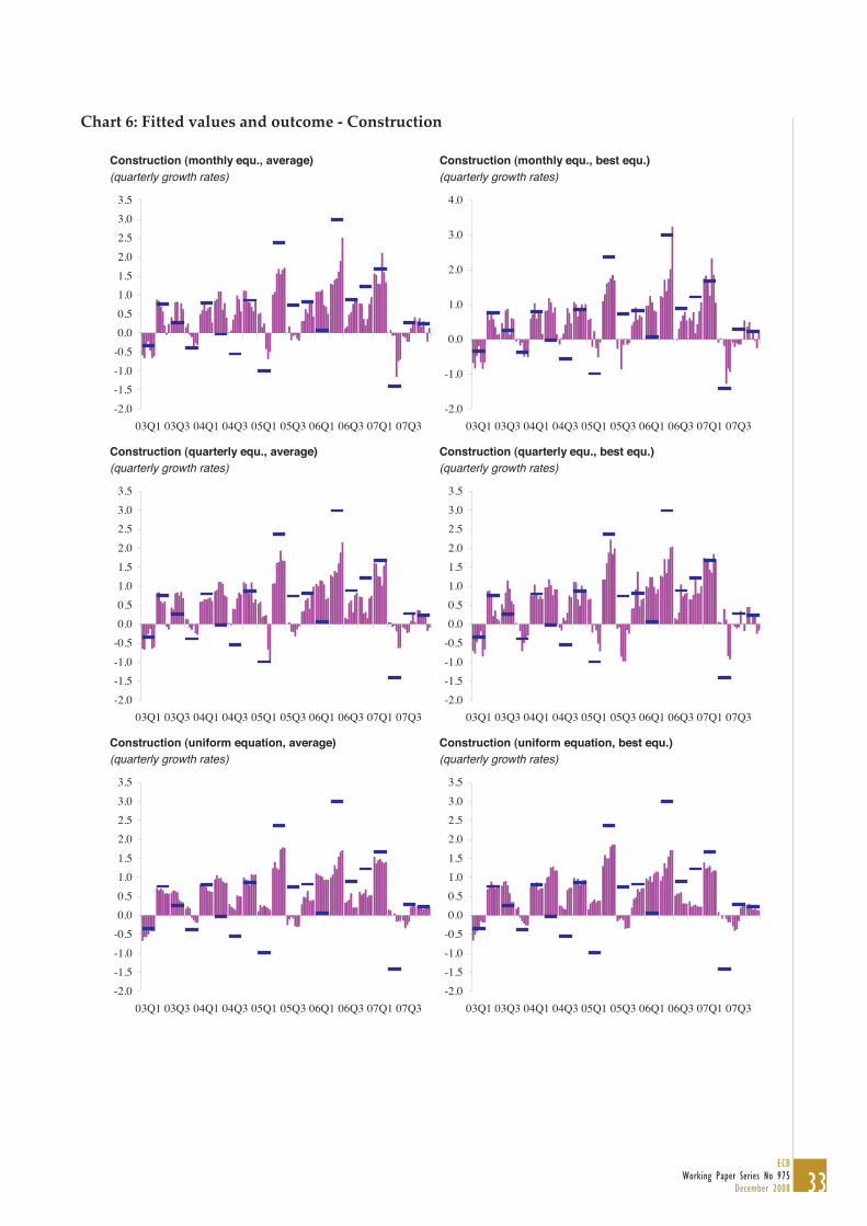
Charts 5 to 13 show the fitted values from our mixture of in and out of sample forecast

procedure together with the final outcomes across all components as well as GDP over the

period 2003Q1 to 2007Q4. They illustrate how the fitted values have evolved over the seven

months of the forecast cycle for both the respective average forecast (left hand side) and the

best equation forecast (right hand side) across the three cases of the monthly, quarterly and

uniform equations.

The main insights from visual inspection of these charts can be summarised as follows: First,

in many cases the fitted values tend to approach the outcomes over the forecast cycle as more

information becomes available. But there are also opposite cases. Second, the charts tend to

confirm the generally better performance of the monthly and quarterly equations compared

25ECB


with the uniform equations. Third, no clear differences are visible as regards the

performance of the best equation and the average forecast. There may be, however,

sometimes a somewhat higher volatility of the best equation forecasts over the cycle. This

could tentatively imply that in practice the average forecasts might be preferred to the best

equation ones in order to gain somewhat more robust and stable results. The same could,

fourth, apply also to the choice of whether to use the monthly or quarterly equations. While

the forecast accuracy of the monthly equations was somewhat better than that of the

quarterly equations, their volatility appears slightly higher which could make the quarterly

equations more appealing in practice. Fifth, a comparison of the charts across sectors,

highlights again the differences in the magnitude of the RMSEs across sectors with larger

forecast errors e.g. for agricultural and construction activity and relatively lower errors for

the services sectors, related also to the differences in volatility in quarterly growth in these

sectors. It also shows the stronger improvements over the forecast cycle for instance in

industry compared with services, related to hard data further improving forecasts of

industrial value added growth at the end of the cycle and a lack of this effect for services.

Finally, all of the above mentioned general features are also visible in the two charts for

GDP, of which one is based on the forecast for total services and the other on the forecasts for

the main services sub sectors. Again, reflecting the only marginal differences in the RMSEs

between these two approaches, a decision on which one of the two to prefer to the other is

not possible from the charts.

Overall, while the outcomes of the forecast exercise clearly show that changing the set of

equations over the forecast cycle appears superior to keeping the same set of equations,

future practical experience with the equations needs to solve the outstanding questions, i.e.,

in particular, whether to use the monthly or quarterly equations and whether to include the

direct forecast for total services or the indirect one via its sub components in the GDP

forecast.

4. Conclusions

This paper develops a forecasting framework for euro area real GDP growth based on a

bottom up approach from the production side. The process of selecting the best performing

equations is accomplished as a pseudo real time forecasting exercise, i.e. due account is taken


of the pattern of available monthly variables over the forecast cycle. Moreover, by applying a

very systematic procedure the best performing equations are selected from a pool of

thousands of test bridge equations. Our modelling approach, finally, includes a novelty

which should be of particular interest to practitioners. We explore whether over the forecast

cycle faced by practitioners, when GDP in a particular quarter has to be repeatedly forecast

based on different sets of available information, the same set of equations or different ones

should be used. Differences in data characteristics suggest that the relative merit of the

included monthly indicators may change over time, which should find its reflection in the

bridge equations.

The results show that all models selected in this forecast exercise clearly outperform the

benchmark models. The variables included in the best equations, that are specifically selected

to forecast value added at particular stages over the forecast cycle, vary substantially over

the cycle pointing to clear changes in the relative importance of individual variables over

time. A general observation is, for instance, that survey information appears of particular

value at the early stages of the forecast cycle, while hard data, such as industrial production,

which are quite volatile but show a high degree of co movement with quarterly value added

growth, are very important only at the latest stages of the forecast cycle. In line with this, it

clearly turns out that the forecast accuracy is higher for the equations that are more

specifically selected to forecast GDP at particular stages over the forecast cycle compared to

the set of selected best equations that are kept unchanged over the whole cycle. This

confirms the conjecture that changing the set of equations over the forecast cycle is superior

to keeping the same equations over time. Comparing the forecast performance of the bridge

equations across branches of activity, it turns out that the magnitude of the RMSEs varies

substantially across sectors. Probably related to differences in the volatility of the data, the

RMSEs are clearly higher in the construction and industrial sectors than in the services

sectors. At the same time, however, the improvement in the forecast accuracy over the cycle

is smaller in services than in industry and construction, which most likely reflects in

particular the scarcity and quality of monthly hard data in services compared to industry

and construction.

Overall, this paper provides a new ingredient to the forecast toolbox for euro area GDP by

extending the bridge equation analysis to the production side of national accounts.

27ECB


Moreover, by introducing the idea of changing forecast equations over the forecast cycle and

thereby aligning the forecast framework closer to the relative information content of the

underlying data, it also adds more generally to the forecast literature. More specifically, this

paper may be seen as a first major step in developing the bottom up euro area GDP early

estimates from the production side. A second not less important step ahead would entail

revisiting the extrapolations of the monthly conjunctural indicators. As the quality of these

extrapolations is vital for the overall performance of the early estimates for GDP, additional

efforts in that direction could help to increase the forecast performance further. Of course, if

the forecasts of variables such as industrial production could be improved further, also the

relative importance of the variables in the equations could change and the process of

selecting the best equations would need to be revisited. We leave this issue for future

research.


References

Altissimo, F., Cristadoro, R., Forni, M., Lippi, M. and G. Veronese (2007), “New EuroCOIN:

tracking economic growth in real time”, CEPR Discussion Paper 5633.

Angelini, E., Banbura, M. and G. Rünstler (2008), “Estimating and forecasting the euro area

monthly national accounts from a dynamic factor model”, ECB Working Paper No. 953,

October 2008.

Angelini, E., Camba Mendez, G. , Giannone, D. , Reichlin, L. and G. Rünstler (2008), “Short

term forecasts of euro area GDP”, CEPR Discussion Paper 6746.

Baffigi, A., Golinelli, R. and G. Parigi (2002), “Real time GDP forecasting in the euro area”,

Banca d’Italia Discussion Paper No. 456, March 2002.

Banbura, M. and G. Rünstler (2007), “A look into the factor model black box: Publication lags

and the role of hard and soft data in forecasting GDP”, ECB Working Paper No. 751.

Camacho, M. and G. Perez Quiros (2008), “Introducting the Euro STING: Short term

indicator of euro area growth”, Working Paper No. 0807, Banco de Espana.

Diron, M. (2008), “Short term forecasts of euro area real GDP growth – An assessment of

real time performance based on vintage data”, Journal of Forecasting, Vol. 27, pp. 371

390.

ECB (2008), “Short term forecasts of economic activity in the euro area”, ECB Monthly

Bulletin, April.

Giannone, D., Reichlin, L. and D. H. Small (2006), “Nowcasting GDP and inflation – The real

time informational content of macroeconomic data releases”, ECB Working Paper No.

633.

Parigi, G. and G. Schlitzer (1995), ”Quarterly Forecasts of the Italian Business Cycle by Means

of Monthly Economic Indicators”, Journal of Forecasting, Vol. 14, pp. 117 – 141.

Rünstler, G. and F. Sédillot (2003), “Short term estimates of euro area real GDP by means of

monthly data”, ECB Working Paper No. 276.

29ECB


Appendix A: Charts

Chart 1: GDP breakdown by branches of activity and applied forecast approaches

AgricultureIndustry excl. constructionConstructionServices

- trade and transportation services- financial and business services- other services

Taxes less subsidies on products

Bridge equations where monthly indicators available

Other forecastapproaches applied for remaining components

Chart 2: Example of forecast cycle for GDP in 2008Q2

2008Q1 2008Q2 2008Q3

Jan. Feb. March Sept.April May June July Aug.

1st fcst 2nd 3rd 4th 5th 6th 7th(1) Uniform equations

(2) Monthly equations

M2NQ M3NQ M1CQ M2CQ M3CQ M1LQ M2LQ(3) Quarterly equations

NQ CQ LQ

U


Chart 3: RMSEs across branches of activity over the forecast cycle

Industry excl. constr. Construction

Financial and business services Trade and transportation services

Total services - direct Total services - indirect

GDP - services direct GDP - services indirect

Note: For the bridge equations, the first (second) bar of each colour shows the best (average of 10 best)equation(s). For the AR, the first (second) bar shows an AR1 (AR4).

0.0

0.1

0.2

0.3

0.4

0.5

0.6

0.7

M 2 M 3 M 1 M 2 M 3 M 1 M 2

Next quarter Current quarter Last quarter

Monthly Quarterly Uniform AR

0.0

0.2

0.4

0.6

0.8

1.0

1.2

M 2 M 3 M 1 M 2 M 3 M 1 M 2



0.0

0.1

0.2

0.3

0.4

M 2 M 3 M 1 M 2 M 3 M 1 M 2



0.00.10.20.30.40.50.60.70.80.91.01.1

M2 NQ M3 NQ M1 CQ M2 CQ M3 CQ M1 LQ M2 LQ

Monthly Quarterly Uniform #REF!

0.0

0.1

0.2

0.3

0.4

M 2 M 3 M 1 M 2 M 3 M 1 M 2



0.0

0.1

0.2

0.3

M 2 M 3 M 1 M 2 M 3 M 1 M 2



0.0

0.1

0.2

0.3

M 2 M 3 M 1 M 2 M 3 M 1 M 2



0.0

0.1

0.2

0.3

M 2 M 3 M 1 M 2 M 3 M 1 M 2



0.0

0.1

0.2

0.3

M 2 M 3 M 1 M 2 M 3 M 1 M 2



31ECB


Chart 4: Comparison of RMSEs: direct versus indirect approach for services and GDP

Services - direct versus indirect (average) GDP - direct versus indirect services (average)

Note: First (second) bar of each colour: direct (indirect) approach

0.0

0.1

0.2

0.3

M 2 M 3 M 1 M 2 M 3 M 1 M 2


Monthly Quarterly Uniform

0.0

0.1

0.2

M 2 M 3 M 1 M 2 M 3 M 1 M 2


Monthly Quarterly Uniform


Chart 5: Fitted values and outcome – Industry (excluding construction)

Industry excl. constr. (monthly equ., average) Industry excl. constr. (monthly equ., best equ.)(quarterly growth rates) (quarterly growth rates)

Industry excl. constr. (quarterly equ., average) Industry excl. constr. (quarterly equ., best equ.)(quarterly growth rates) (quarterly growth rates)

Industry excl. constr. (uniform equation, average) Industry excl. constr. (uniform equation, best equ.)(quarterly growth rates) (quarterly growth rates)

-1.5

-1.0

-0.5

0.0

0.5

1.0

1.5

2.0

03Q1 03Q3 04Q1 04Q3 05Q1 05Q3 06Q1 06Q3 07Q1 07Q3-1.5

-1.0

-0.5

0.0

0.5

1.0

1.5

2.0

03Q1 03Q3 04Q1 04Q3 05Q1 05Q3 06Q1 06Q3 07Q1 07Q3

-1.5

-1.0

-0.5

0.0

0.5

1.0

1.5

2.0

03Q1 03Q3 04Q1 04Q3 05Q1 05Q3 06Q1 06Q3 07Q1 07Q3-1.5

-1.0

-0.5

0.0

0.5

1.0

1.5

2.0

03Q1 03Q3 04Q1 04Q3 05Q1 05Q3 06Q1 06Q3 07Q1 07Q3

-1.5

-1.0

-0.5

0.0

0.5

1.0

1.5

2.0

03Q1 03Q3 04Q1 04Q3 05Q1 05Q3 06Q1 06Q3 07Q1 07Q3-1.5

-1.0

-0.5

0.0

0.5

1.0

1.5

2.0

03Q1 03Q3 04Q1 04Q3 05Q1 05Q3 06Q1 06Q3 07Q1 07Q3

33ECB


Chart 6: Fitted values and outcome Construction

Construction (monthly equ., average) Construction (monthly equ., best equ.)(quarterly growth rates) (quarterly growth rates)

Construction (quarterly equ., average) Construction (quarterly equ., best equ.)(quarterly growth rates) (quarterly growth rates)

Construction (uniform equation, average) Construction (uniform equation, best equ.)(quarterly growth rates) (quarterly growth rates)

-2.0

-1.5-1.0

-0.5

0.00.5

1.01.5

2.0

2.53.0

3.5

03Q1 03Q3 04Q1 04Q3 05Q1 05Q3 06Q1 06Q3 07Q1 07Q3-2.0

-1.0

0.0

1.0

2.0

3.0

4.0

03Q1 03Q3 04Q1 04Q3 05Q1 05Q3 06Q1 06Q3 07Q1 07Q3

-2.0

-1.5-1.0

-0.5

0.00.5

1.01.5

2.0

2.53.0

3.5

03Q1 03Q3 04Q1 04Q3 05Q1 05Q3 06Q1 06Q3 07Q1 07Q3-2.0

-1.5-1.0

-0.5

0.00.5

1.01.5

2.0

2.53.0

3.5

03Q1 03Q3 04Q1 04Q3 05Q1 05Q3 06Q1 06Q3 07Q1 07Q3

-2.0

-1.5-1.0

-0.5

0.00.5

1.01.5

2.0

2.53.0

3.5

03Q1 03Q3 04Q1 04Q3 05Q1 05Q3 06Q1 06Q3 07Q1 07Q3-2.0

-1.5-1.0

-0.5

0.00.5

1.01.5

2.0

2.53.0

3.5

03Q1 03Q3 04Q1 04Q3 05Q1 05Q3 06Q1 06Q3 07Q1 07Q3


Chart 7: Fitted values and outcome – Services (direct)

Services, direct (monthly equ., average) Services, direct (monthly equ., best equ.)(quarterly growth rates) (quarterly growth rates)

Services, direct (quarterly equ., average) Services, direct (quarterly equ., best equ.)(quarterly growth rates) (quarterly growth rates)

Services, direct (uniform equation, average) Services, direct (uniform equation, best equ.)(quarterly growth rates) (quarterly growth rates)

0.0

0.2

0.4

0.6

0.8

1.0

1.2

03Q1 03Q3 04Q1 04Q3 05Q1 05Q3 06Q1 06Q3 07Q1 07Q30.0

0.2

0.4

0.6

0.8

1.0

1.2

03Q1 03Q3 04Q1 04Q3 05Q1 05Q3 06Q1 06Q3 07Q1 07Q3

0.0

0.2

0.4

0.6

0.8

1.0

1.2

03Q1 03Q3 04Q1 04Q3 05Q1 05Q3 06Q1 06Q3 07Q1 07Q30.0

0.2

0.4

0.6

0.8

1.0

1.2

03Q1 03Q3 04Q1 04Q3 05Q1 05Q3 06Q1 06Q3 07Q1 07Q3

0.0

0.2

0.4

0.6

0.8

1.0

1.2

03Q1 03Q3 04Q1 04Q3 05Q1 05Q3 06Q1 06Q3 07Q1 07Q30.0

0.2

0.4

0.6

0.8

1.0

1.2

03Q1 03Q3 04Q1 04Q3 05Q1 05Q3 06Q1 06Q3 07Q1 07Q3

35ECB


Chart 8: Fitted values and outcome – Trade and transportation services

Trade and transp. services (monthly equ., average) Trade and transp. services (monthly equ., best equ.)(quarterly growth rates) (quarterly growth rates)

Trade and transp. services (quarterly equ., average) Trade and transp. services (quarterly equ., best equ.)(quarterly growth rates) (quarterly growth rates)

Trade and transp. services (uniform equation, average) Trade and transp. services (uniform equation, best equ.)(quarterly growth rates) (quarterly growth rates)

-0.2

0.0

0.2

0.4

0.6

0.8

1.0

1.2

1.4

03Q1 03Q3 04Q1 04Q3 05Q1 05Q3 06Q1 06Q3 07Q1 07Q3-0.4

-0.2

0.0

0.2

0.4

0.6

0.8

1.0

1.2

1.4

03Q1 03Q3 04Q1 04Q3 05Q1 05Q3 06Q1 06Q3 07Q1 07Q3

-0.2

0.0

0.2

0.4

0.6

0.8

1.0

1.2

1.4

03Q1 03Q3 04Q1 04Q3 05Q1 05Q3 06Q1 06Q3 07Q1 07Q3-0.2

0.0

0.2

0.4

0.6

0.8

1.0

1.2

1.4

03Q1 03Q3 04Q1 04Q3 05Q1 05Q3 06Q1 06Q3 07Q1 07Q3

-0.2

0.0

0.2

0.4

0.6

0.8

1.0

1.2

1.4

03Q1 03Q3 04Q1 04Q3 05Q1 05Q3 06Q1 06Q3 07Q1 07Q3-0.2

0.0

0.2

0.4

0.6

0.8

1.0

1.2

1.4

03Q1 03Q3 04Q1 04Q3 05Q1 05Q3 06Q1 06Q3 07Q1 07Q3


Chart 9: Fitted values and outcome – Financial and business services

Fin. and bus. services (monthly equ., average) Fin. and bus. services (monthly equ., best equ.)(quarterly growth rates) (quarterly growth rates)

Fin. and bus. services (quarterly equ., average) Fin. and bus. services (quarterly equ., best equ.)(quarterly growth rates) (quarterly growth rates)

Fin. and bus. services (uniform equation, average) Fin. and bus. services (uniform equation, best equ.)(quarterly growth rates) (quarterly growth rates)

-0.2

0.0

0.2

0.4

0.6

0.8

1.0

1.2

1.4

03Q1 03Q3 04Q1 04Q3 05Q1 05Q3 06Q1 06Q3 07Q1 07Q3-0.2

0.0

0.2

0.4

0.6

0.8

1.0

1.2

1.4

03Q1 03Q3 04Q1 04Q3 05Q1 05Q3 06Q1 06Q3 07Q1 07Q3

-0.2

0.0

0.2

0.4

0.6

0.8

1.0

1.2

1.4

03Q1 03Q3 04Q1 04Q3 05Q1 05Q3 06Q1 06Q3 07Q1 07Q3-0.2

0.0

0.2

0.4

0.6

0.8

1.0

1.2

1.4

03Q1 03Q3 04Q1 04Q3 05Q1 05Q3 06Q1 06Q3 07Q1 07Q3

-0.2

0.0

0.2

0.4

0.6

0.8

1.0

1.2

1.4

03Q1 03Q3 04Q1 04Q3 05Q1 05Q3 06Q1 06Q3 07Q1 07Q3-0.2

0.0

0.2

0.4

0.6

0.8

1.0

1.2

1.4

03Q1 03Q3 04Q1 04Q3 05Q1 05Q3 06Q1 06Q3 07Q1 07Q3

37ECB


Chart 10: Fitted values and outcome – Services (indirect)

Services (indirect) (monthly equ., average) Services (indirect) (monthly equ., best equ.)(quarterly growth rates) (quarterly growth rates)

Services (indirect) (quarterly equ., average) Services (indirect) (quarterly equ., best equ.)(quarterly growth rates) (quarterly growth rates)

Services (indirect) (uniform equation, average) Services (indirect) (uniform equation, best equ.)(quarterly growth rates) (quarterly growth rates)

0.0

0.2

0.4

0.6

0.8

1.0

1.2

03Q1 03Q3 04Q1 04Q3 05Q1 05Q3 06Q1 06Q3 07Q1 07Q3-0.2

0.0

0.2

0.4

0.6

0.8

1.0

1.2

03Q1 03Q3 04Q1 04Q3 05Q1 05Q3 06Q1 06Q3 07Q1 07Q3

0.0

0.2

0.4

0.6

0.8

1.0

1.2

03Q1 03Q3 04Q1 04Q3 05Q1 05Q3 06Q1 06Q3 07Q1 07Q3-0.2

0.0

0.2

0.4

0.6

0.8

1.0

1.2

03Q1 03Q3 04Q1 04Q3 05Q1 05Q3 06Q1 06Q3 07Q1 07Q3

0.0

0.2

0.4

0.6

0.8

1.0

1.2

03Q1 03Q3 04Q1 04Q3 05Q1 05Q3 06Q1 06Q3 07Q1 07Q30.0

0.2

0.4

0.6

0.8

1.0

1.2

03Q1 03Q3 04Q1 04Q3 05Q1 05Q3 06Q1 06Q3 07Q1 07Q3


Chart 11: Fitted values and outcome – Agriculture, other services and taxes less subsidies

on products

Agriculture Other services(quarterly growth rates) (quarterly growth rates)

Taxes less subsidies on products(quarterly growth rates)

-8.0

-6.0

-4.0

-2.0

0.0

2.0

4.0

6.0

8.0

02Q1 02Q4 03Q3 04Q2 05Q1 05Q4 06Q3 07Q2

fitted observed

0.0

0.1

0.2

0.3

0.4

0.5

0.6

0.7

02Q1 02Q4 03Q3 04Q2 05Q1 05Q4 06Q3 07Q2

fitted observed

-1.5

-1.0

-0.5

0.0

0.5

1.0

1.5

2.0

02Q1 02Q4 03Q3 04Q2 05Q1 05Q4 06Q3 07Q2

fitted observed

39ECB


Chart 12: Fitted values and outcome – GDP (using direct forecast for services)

GDP (with direct services) (monthly equ., average) GDP (with direct services) (monthly equ., best equ.)(quarterly growth rates) (quarterly growth rates)

GDP (with direct services) (quarterly equ., average) GDP (with direct services) (quarterly equ., best equ.)(quarterly growth rates) (quarterly growth rates)

GDP (with direct services) (uniform equation, average) GDP (with direct services) (uniform equation, best equ.)(quarterly growth rates) (quarterly growth rates)

-0.2

0.0

0.2

0.4

0.6

0.8

1.0

1.2

03Q1 03Q3 04Q1 04Q3 05Q1 05Q3 06Q1 06Q3 07Q1 07Q3-0.2

0.0

0.2

0.4

0.6

0.8

1.0

1.2

03Q1 03Q3 04Q1 04Q3 05Q1 05Q3 06Q1 06Q3 07Q1 07Q3

-0.4

-0.2

0.0

0.2

0.4

0.6

0.8

1.0

1.2

03Q1 03Q3 04Q1 04Q3 05Q1 05Q3 06Q1 06Q3 07Q1 07Q3-0.4

-0.2

0.0

0.2

0.4

0.6

0.8

1.0

1.2

03Q1 03Q3 04Q1 04Q3 05Q1 05Q3 06Q1 06Q3 07Q1 07Q3

-0.2

0.0

0.2

0.4

0.6

0.8

1.0

1.2

03Q1 03Q3 04Q1 04Q3 05Q1 05Q3 06Q1 06Q3 07Q1 07Q3-0.2

0.0

0.2

0.4

0.6

0.8

1.0

1.2

03Q1 03Q3 04Q1 04Q3 05Q1 05Q3 06Q1 06Q3 07Q1 07Q3


Chart 13: Fitted values and outcome – GDP (using indirect forecast for services)

GDP (with indirect services) (monthly equ., average) GDP (with indirect services) (monthly equ., best equ.)(quarterly growth rates) (quarterly growth rates)

GDP (with indirect services) (quarterly equ., average) GDP (with indirect services) (quarterly equ., best equ.)(quarterly growth rates) (quarterly growth rates)

GDP (with indirect services) (uniform equation, average) GDP (with indirect services) (uniform equation, best equ.)(quarterly growth rates) (quarterly growth rates)

-0.4

-0.2

0.0

0.2

0.4

0.6

0.8

1.0

1.2

03Q1 03Q3 04Q1 04Q3 05Q1 05Q3 06Q1 06Q3 07Q1 07Q3-0.4

-0.2

0.0

0.2

0.4

0.6

0.8

1.0

1.2

03Q1 03Q3 04Q1 04Q3 05Q1 05Q3 06Q1 06Q3 07Q1 07Q3

-0.4

-0.2

0.0

0.2

0.4

0.6

0.8

1.0

1.2

03Q1 03Q3 04Q1 04Q3 05Q1 05Q3 06Q1 06Q3 07Q1 07Q3-0.4

-0.2

0.0

0.2

0.4

0.6

0.8

1.0

1.2

03Q1 03Q3 04Q1 04Q3 05Q1 05Q3 06Q1 06Q3 07Q1 07Q3

-0.2

0.0

0.2

0.4

0.6

0.8

1.0

1.2

03Q1 03Q3 04Q1 04Q3 05Q1 05Q3 06Q1 06Q3 07Q1 07Q3-0.2

0.0

0.2

0.4

0.6

0.8

1.0

1.2

03Q1 03Q3 04Q1 04Q3 05Q1 05Q3 06Q1 06Q3 07Q1 07Q3

41ECB


Appendix B: Tables

Table 1: List of pre selected variables for industry (excluding construction)


Table 2: List of pre selected variables for construction

Table 3: List of pre selected variables for services

43ECB


List of pre selected variables for financial and business services

Table 4: List of pre selected variables for trade and transportation services

Table 5:


Table 6: Selected equations for industry (excluding construction)

Lags

of d

epen

dent

var

iabl

e

Ind.

pro

d. (e

xcl.

cons

tr.)

Ind.

pro

d. c

onsu

mer

Ind.

pro

d. e

nerg

y

Ind.

pro

d. in

term

.

Ind.

pro

d. c

apita

l

New

ord

ers

Impo

rts in

term

. goo

ds

Impo

rts m

anuf

. goo

ds

Impo

rts to

tal

Expo

rts in

term

. goo

ds

Expo

rts m

anuf

. goo

ds

Expo

rts to

tal

NEE

R

NEE

R

Oil

pric

es

Oil

pric

es

Une

mpl

oym

ent

Une

mpl

oym

ent

EC c

onsu

mer

con

f.

EC c

onsu

mer

goo

ds

EC in

d. c

onf.

elec

t. m

ach.

EC in

d. c

onf.

inte

rm.

EC in

d. c

onf.

tota

l

EC in

d. c

onf.

capi

tal

EC in

d. c

onf.

min

. goo

ds

EC in

d. c

onf.

pulp

EC in

d. c

onf.

of te

xtile

s

Econ

omic

Sen

t. In

dic.

PMI c

hem

ical

s

PMI c

oke,

che

m.,

rubb

er

PMI c

ompo

site

outp

ut

PMI i

nter

med

iate

goo

ds

PMI m

achi

nery

PMI m

anuf

.

PMI r

ubbe

r

PMI s

erv.

bus

. act

ivity

inde

x

lags of indic. 0 0 0 0 0 0 0 0 0 0 0 0 0 1 0 1 0 1 0 0 0 0 0 0 0 0 0 0 0 0 0 0 0 0 0 0M2NQ 1 0 x x x

2 0 x x3 0 x x x x4 0 x x x5 0 x x x x6 0 x x x7 0 x x x8 0 x x x x9 0 x x x x10 0 x x x

M3NQ 1 0 x x x2 0 x x x x3 0 x x x x4 0 x x x5 0 x x x x6 0 x x x x7 0 x x x x8 0 x x x x9 0 x x x x10 0 x x x x

M1CQ 1 0 x x x x2 0 x x x3 0 x x x x4 0 x x x x5 0 x x x x6 0 x x x7 0 x x x x8 0 x x x x9 0 x x x x10 0 x x x x

M2CQ 1 0 x x x x2 0 x x x x3 0 x x x x4 0 x x x x5 0 x x x x6 0 x x x x7 0 x x x x8 0 x x x x9 0 x x x x10 0 x x x x

M3CQ 1 0 x x x x2 0 x x x x3 0 x x x x4 0 x x x x5 0 x x x x6 0 x x x7 0 x x x x8 0 x x x x9 0 x x x x10 0 x x x x

M1LQ 1 0 x x x x2 0 x x x x3 0 x x x x4 0 x x x x5 0 x x x x6 0 x x x x7 0 x x x x8 0 x x x x9 0 x x x x10 0 x x x x


NQ 1 0 x x x2 0 x x3 0 x x x x4 0 x x x5 0 x x x x6 0 x x x x7 0 x x x8 0 x x x x9 0 x x x10 0 x x x

CQ 1 0 x x x x2 0 x x x x3 0 x x x x4 0 x x x x5 0 x x x x6 0 x x x x7 0 x x x x8 0 x x x x9 0 x x x x10 0 x x x x

LQ 1 0 x x x x2 0 x x x x3 0 x x x x4 0 x x x x5 0 x x x x6 0 x x x x7 0 x x x x8 0 x x x x9 0 x x x x10 0 x x x x

U 1 0 x x x x2 0 x x x x3 0 x x x x4 0 x x x x5 0 x x x x6 0 x x x x7 0 x x x x8 0 x x x x9 0 x x x x10 0 x x x x

45ECB


Table 7: Selected equations for construction

Lags

of d

epen

dent

var

iabl

e

Cons

tr. p

rodu

ctio

n

New

ord

ers c

onstr

.

New

ord

ers c

onstr

.

New

ord

ers c

onstr

.

New

ord

ers c

onstr

.

Build

ing

perm

its

Build

ing

perm

its

Build

ing

perm

its

Build

ing

perm

its

Impo

rts in

term

. goo

ds

NEE

R

NEE

R

Une

mpl

oym

ent

Une

mpl

oym

ent

EC c

onstr

. con

f.

EC c

onstr

. con

f.

EC c

onstr

. con

f.

PMI c

onstr

. out

put

PMI r

eale

est

ate

etc.

PMI r

eale

est

ate

etc.

lags of indic. 0 0 1 2 3 0 1 2 3 0 0 1 0 1 0 1 2 0 0 1M2NQ 1 1 x x x x

2 1 x x x x3 1 x x x x4 1 x x x x5 1 x x x x6 1 x x x x7 1 x x x x8 1 x x x9 1 x x x x10 1 x x x x

M3NQ 1 1 x x x x2 1 x x x x3 1 x x x x4 1 x x x x5 1 x x x x6 1 x x x x7 1 x x x x8 1 x x x9 1 x x x x10 1 x x x


M2CQ 1 1 x x x x2 1 x x x x3 1 x x x x4 1 x x x x5 1 x x x x6 1 x x x x7 1 x x x x8 1 x x x x9 1 x x x x10 1 x x x


M1LQ 1 1 x x x x2 1 x x x x3 1 x x x x4 1 x x x x5 1 x x x x6 1 x x x x7 1 x x x x8 1 x x x x9 1 x x x x10 1 x x x


NQ 1 1 x x x x2 1 x x x x3 1 x x x x4 1 x x x x5 1 x x x x6 1 x x x x7 1 x x x x8 1 x x x x9 1 x x x x10 1 x x x x

CQ 1 1 x x x x2 1 x x x x3 1 x x x x4 1 x x x x5 1 x x x x6 1 x x x x7 1 x x x x8 1 x x x9 1 x x x x10 1 x x x x

LQ 1 1 x x x x2 1 x x x x3 1 x x x x4 1 x x x x5 1 x x x x6 1 x x x x7 1 x x x x8 1 x x x x9 1 x x x x10 1 x x x x

U 1 1 x x x x2 1 x x x x3 1 x x x x4 1 x x x x5 1 x x x x6 1 x x x x7 1 x x x x8 1 x x x x9 1 x x x x10 1 x x x x


Table 8: Selected equations for services

Lags

of d

epen

dent

var

iabl

e

Reta

il sa

les h

ouse

h. e

quip

.

Turn

over

: who

lesa

le tr

ade

Impo

rts in

term

. goo

ds

Impo

rts in

term

. goo

ds

Impo

rts m

anuf

. goo

ds

Impo

rts m

anuf

. goo

ds

Impo

rts m

anuf

. goo

ds

Impo

rts to

tal

Impo

rts to

tal

Expo

rts in

term

. goo

ds

Expo

rts m

anuf

. goo

ds

Expo

rts to

tal

NEE

R

NEE

R

NEE

R

Une

mpl

oym

ent

Une

mpl

oym

ent

EC c

onsu

mer

con

f.

EC in

d. c

onf.

tota

l

EC in

d. c

onf.

tota

l

EC se

rv re

cent

dem

and

EC se

rvic

es c

onfid

ence

Econ

omic

Sen

t. In

dic.

Econ

omic

Sen

t. In

dic.

PMI c

ompo

site

out

put

PMI c

ompo

site

out

put

PMI f

inan

cial

inte

rm.

PMI h

otel

resta

uran

ts

PMI l

and,

wat

er, a

ir tra

nspo

rt

PMI m

anuf

.

PMI m

anuf

.

PMI o

ther

serv

. bus

. act

.

PMI r

eal e

state

(sm

alle

r)

PMI s

erv.

bus

. act

ivity

inde

x

PMI t

rans

porta

tion

PMI l

and

trans

porta

tion

lags of indic. 0 0 1 2 0 1 2 1 2 1 0 1 0 1 2 0 1 0 0 1 0 0 0 1 0 1 0 0 0 0 1 0 0 0 0 0M2NQ 1 2 x x x x

2 1 x x x x3 2 x x x x4 1 x x x x5 2 x x x x6 2 x x x x7 1 x x x x8 2 x x x x9 2 x x x x

10 1 x x x xM3NQ 1 2 x x x x


10 2 x x x xM1CQ 1 2 x x x x


10 2 x x x xM2CQ 1 2 x x x x


10 0 x x x xM3CQ 1 2 x x x x


10 2 x x x xM1LQ 1 1 x x x x


10 1 x x x xM2LQ 1 2 x x x x


10 1 x x x xNQ 1 2 x x x x


10 1 x x x xCQ 1 2 x x x x


10 2 x x x xLQ 1 1 x x x x


10 1 x x x xU 1 2 x x x x


10 2 x x x x

47ECB


Table 9: Selected equations for trade and transportation services

Lags

of d

epen

dent

var

iabl

e

Reta

il sa

les

Reta

il sa

les h

ouse

h. e

quip

.

Turn

over

: who

lesa

le h

h go

ods

Turn

over

: who

lesa

le h

h go

ods

Turn

over

: who

lesa

le h

h go

ods

Turn

over

: who

lesa

le tr

ade

Turn

over

: who

lesa

le tr

ade

Turn

over

: who

lesa

le tr

ade

Oil

pric

es

Oil

pric

es

Oil

pric

es

NEE

R

NEE

R

NEE

R

Une

mpl

oym

ent

Une

mpl

oym

ent

EC c

onsu

mer

con

f.

EC in

d. c

onf.

tota

l

EC se

rv re

cent

dem

and

EC se

rvic

es c

onfid

ence

Econ

omic

Sen

t. In

dic.

PMI c

ompo

site

outp

ut

PMI f

inan

cial

inte

rm.

PMI h

otel

rest

aura

nts

PMI l

and,

wat

er, a

ir tra

nspo

rt

PMI m

anuf

.

PMI o

ther

serv

. bus

. act

.

PMI r

eal e

state

(sm

alle

r)

PMI s

erv.

bus

. act

ivity

inde

x

PMI t

rans

porta

tion

PMI l

and

trans

porta

tion

lags of indic. 0 0 0 1 2 0 1 2 0 1 2 0 1 2 0 1 0 0 0 0 0 0 0 0 0 0 0 0 0 0 0M2NQ 1 0 x x x x


10 1 x x x xM3NQ 1 0 x x x x


10 0 x x x xM1CQ 1 0 x x x x


10 0 x x x xM2CQ 1 1 x x x x


10 0 x x x xM3CQ 1 0 x x x x


10 1 x x x xM1LQ 1 0 x x x x


10 0 x x x xM2LQ 1 0 x x x x


10 1 x x x xNQ 1 0 x x x x


10 1 x x x xCQ 1 1 x x x x


10 0 x x x xLQ 1 0 x x x x


10 1 x x x xU 1 1 x x x x


10 1 x x x x


Table 10: Selected equations for financial and business services

Lags

of d

epen

dent

var

iabl

e

Oil

pric

es

NEE

R

NEE

R

Une

mpl

oym

ent

Une

mpl

oym

ent

EC c

onsu

mer

con

f.

EC in

d. c

onf.

tota

l

EC se

rv re

cent

dem

and

EC se

rvic

es c

onfid

ence

Econ

omic

Sen

t. In

dic.

PMI c

ompo

site

outp

ut

PMI c

ompo

site

outp

ut

PMI f

inan

cial

inte

rm.

PMI f

inan

cial

inte

rm.

PMI c

ompu

ters

PMI m

anuf

.

PMI o

ther

serv

. bus

. act

.

PMI o

ther

serv

. bus

. act

.

PMI r

eal e

stat

e (s

mal

ler)

PMI r

eal e

stat

e (s

mal

ler)

PMI r

eale

esta

te e

tc.

PMI s

erv.

bus

. act

ivity

inde

x

lags of indic. 0 0 1 0 1 0 0 0 0 0 0 1 0 1 0 0 0 1 0 1 0 0M2NQ 1 0 x x x x


10 0 x x x xM3NQ 1 0 x x x x


10 0 x x x xM1CQ 1 0 x x x x


10 0 x x x xM2CQ 1 0 x x x x


10 0 x x x xM3CQ 1 0 x x x x


10 0 x x x xM1LQ 1 0 x x x x

2 0 x x x x3 0 x x x x4 0 x x x x5 0 x x x x6 0 x x x x7 0 x x x x8 0 x x x x9 0 x x x

10 0 x x x xM2LQ 1 0 x x x x


10 0 x x x xNQ 1 0 x x x x


10 0 x x x xCQ 1 0 x x x x


10 0 x x x xLQ 1 0 x x x x


10 0 x x x xU 1 0 x x x x


10 0 x x x x

49ECB


Table 11: Selected variables – Industry (excluding construction)

M2NQ 4 0 0 3 0 10 10 0M3NQ 2 0 1 2 10 10 10 0M1CQ 2 0 2 4 9 8 10 2M2CQ 0 0 0 2 2 8 10 8M3CQ 10 0 3 1 1 2 10 10M1LQ 10 0 4 1 10 0 2 10M2LQ 10 0 3 0 10 0 5 10NQ 4 0 0 3 3 10 10 0CQ 2 0 2 2 4 2 10 10LQ 10 0 4 0 10 0 4 10U 4 2 9 0 10 0 3 10

IP New orders Trade NEER Oil prices Unempl. EC

surveys PMI

Table 12: Selected variables – Construction

M2NQ 0 7 5 2 2 0 10 10M3NQ 0 0 4 3 9 0 10 10M1CQ 0 2 10 0 3 2 10 10M2CQ 0 0 10 2 3 0 10 10M3CQ 0 2 10 0 4 0 5 10M1LQ 0 2 10 2 2 0 3 10M2LQ 4 0 10 3 0 3 3 10NQ 0 4 5 4 4 0 10 10CQ 0 1 10 2 2 1 10 10LQ 0 1 10 6 3 0 3 10U 0 4 7 2 2 3 10 10

IPC New orders Build. perm. Trade NEER Unempl. EC surveys PMI

Table 13: Selected variables – Services

M2NQ 0 2 5 8 10 10M3NQ 2 6 0 2 10 8M1CQ 0 5 1 10 9 10M2CQ 1 10 10 9 1 9M3CQ 0 10 10 10 0 10M1LQ 6 7 6 1 1 10M2LQ 3 4 9 4 1 10NQ 5 3 1 8 10 5CQ 1 10 10 10 0 9LQ 6 7 6 1 1 10U 1 10 10 10 0 9

EC surveys PMITurnover Trade NEER Unempl.


Table 14: Selected variables Trade and transportation services

M2NQ 8 3 9 0 5 10M3NQ 5 0 10 0 6 10M1CQ 10 5 4 0 6 10M2CQ 9 0 7 0 5 10M3CQ 8 0 10 0 3 10M1LQ 7 0 10 0 5 10M2LQ 8 0 10 0 4 10NQ 7 0 10 0 5 10CQ 10 0 7 0 7 10LQ 7 0 10 0 4 10U 10 0 10 0 4 10

EC surveys PMITurnover Oil prices NEER Unempl.

Table 15: Selected variables Financial and business services

M2NQ 3 7 0 3 10M3NQ 1 0 3 3 10M1CQ 0 3 1 3 10M2CQ 0 1 3 2 10M3CQ 0 0 1 4 10M1LQ 1 0 2 10 10M2LQ 1 0 2 10 10NQ 1 0 1 4 10CQ 0 2 1 4 10LQ 1 0 2 10 10U 0 4 3 0 10

Oil prices NEER Unempl.EC

surveys PMI

51ECB


Table 16: Summary of frequently selected individual variables

Sector Uniform equationsNQ CQ LQ

Industry EC consumer confidence ESI Industrial production PMI servicesunemployment rate PMI services PMI composite oil pricesoil prices PMI rubber PMI services exportsproduction of energy unemployment rate oil prices prod. of consumer goodsESI EC ind. conf. capital goods

Construction EC construction confidence EC construction confidence PMI construction EC construction confidencePMI real estate, etc. Building permits Building permits Building permitsBuilding permits PMI real estate, etc. PMI real estate, etc. PMI real estate, etc.

Imports intermed. Goods PMI constructionConstruction production

Services EC consumer confidence Imports of intermed. goods Imports of intermed. goods unemployment rateEC services confidence neer neer Imports of intermed. goodsunemployment rate unemployment rate PMI other business services neerTurnover wholesale Turnover wholesale

Trade and transportation neer PMI hotels and rest. neer PMI hotels and rest.PMI real estate etc. neer turnover wholesale neerturnover wholesale turnover wholesale Pmi land, water, air PMI for manufacturingPMI hotels and restaurants EC consumer confidence PMI land transportation turnover wholesaleEC services confidence PMI transportation EC consumer confidence

EC services confidence Financial and business PMI real estate, etc. PMI real estate, etc. PMI composite PMI real estate

PMI computers PMI composite EC consumer confidence PMI compositePMI composite PMI manufacturing PMI other business activities PMI manufacturing

PMI financial intermediation

Forecast cycle


Table 17: RMSE – Industry (excluding construction)

M2 NQ M3 NQ M1 CQ M2 CQ M3 CQ M1 LQ M2 LQ NQ CQ LQ UMonthly equationsEqu1 0.469 0.421 0.422 0.384 0.309 0.241 0.218 0.445 0.375 0.230 0.363Equ2 0.470 0.422 0.423 0.387 0.311 0.243 0.219 0.447 0.377 0.231 0.365Equ3 0.474 0.426 0.429 0.390 0.311 0.248 0.220 0.451 0.380 0.235 0.368Equ4 0.474 0.436 0.429 0.390 0.312 0.249 0.220 0.456 0.380 0.235 0.370Equ5 0.476 0.437 0.430 0.391 0.312 0.250 0.221 0.457 0.381 0.236 0.371Equ6 0.478 0.438 0.431 0.392 0.312 0.250 0.222 0.458 0.381 0.236 0.372Equ7 0.482 0.438 0.431 0.392 0.312 0.250 0.223 0.461 0.382 0.237 0.373Equ8 0.482 0.439 0.432 0.395 0.313 0.250 0.223 0.461 0.383 0.237 0.374Equ9 0.483 0.439 0.432 0.396 0.314 0.252 0.224 0.462 0.384 0.238 0.375Equ10 0.483 0.440 0.432 0.397 0.315 0.252 0.225 0.462 0.385 0.239 0.375Avg 0.476 0.433 0.417 0.373 0.311 0.247 0.219 0.455 0.370 0.234 0.365Quarterly equations

NQ NQ CQ CQ CQ LQ LQ NQ CQ LQ UEqu1 0.490 0.421 0.451 0.396 0.362 0.241 0.218 0.457 0.405 0.230 0.381Equ2 0.470 0.445 0.438 0.405 0.374 0.243 0.220 0.458 0.407 0.232 0.382Equ3 0.491 0.422 0.464 0.413 0.339 0.250 0.220 0.458 0.408 0.236 0.384Equ4 0.469 0.447 0.453 0.407 0.361 0.250 0.222 0.458 0.409 0.236 0.384Equ5 0.490 0.426 0.444 0.423 0.357 0.248 0.224 0.459 0.410 0.237 0.385Equ6 0.474 0.454 0.492 0.391 0.338 0.249 0.226 0.464 0.412 0.238 0.388Equ7 0.474 0.454 0.489 0.417 0.313 0.253 0.223 0.464 0.412 0.238 0.388Equ8 0.476 0.464 0.457 0.422 0.353 0.250 0.225 0.470 0.413 0.238 0.390Equ9 0.478 0.463 0.446 0.417 0.374 0.254 0.223 0.471 0.414 0.239 0.391Equ10 0.483 0.459 0.461 0.421 0.351 0.250 0.227 0.471 0.414 0.239 0.391Avg 0.477 0.439 0.444 0.397 0.331 0.247 0.221 0.458 0.394 0.234 0.377Uniform equations

U U U U U U U U U U UEqu1 0.559 0.506 0.450 0.424 0.363 0.361 0.307 0.533 0.414 0.335 0.432Equ2 0.565 0.503 0.457 0.422 0.353 0.334 0.347 0.535 0.413 0.341 0.434Equ3 0.557 0.507 0.449 0.430 0.375 0.362 0.320 0.532 0.419 0.342 0.435Equ4 0.549 0.515 0.469 0.438 0.375 0.355 0.300 0.532 0.429 0.329 0.437Equ5 0.559 0.514 0.465 0.426 0.372 0.368 0.302 0.537 0.423 0.337 0.437Equ6 0.594 0.529 0.464 0.413 0.339 0.355 0.297 0.563 0.408 0.327 0.439Equ7 0.548 0.516 0.466 0.441 0.383 0.361 0.307 0.532 0.432 0.335 0.439Equ8 0.580 0.523 0.473 0.430 0.348 0.325 0.327 0.552 0.420 0.326 0.439Equ9 0.557 0.512 0.460 0.426 0.374 0.379 0.319 0.535 0.422 0.350 0.439Equ10 0.564 0.520 0.470 0.431 0.368 0.358 0.310 0.543 0.425 0.335 0.440Avg 0.561 0.512 0.458 0.424 0.359 0.347 0.298 0.537 0.416 0.324 0.432Benchmark modelsAR1 0.581 0.581 0.581 0.581 0.567 0.567 0.567 0.581 0.576 0.567 0.575AR4 0.618 0.595 0.595 0.595 0.570 0.570 0.570 0.606 0.587 0.570 0.588naïve 0.780 0.777 0.777 0.777 0.715 0.715 0.715 0.778 0.757 0.715 0.751avg 95-07 0.586 0.586 0.586 0.586 0.586 0.586 0.586 0.586 0.586 0.586 0.586

53ECB


Table 18: RMSE – Construction





Table 19: RMSE – Services – direct approach




55ECB


Table 20: RMSE Trade and transportation services





Table 21: RMSE Financial and business services




57ECB


Table 22: RMSE – Other services

U Lag 3 of dep. var. and dlog of government consumption 0.141

AR1 0.147 AR4 0.144 naïve 0.176 avg 95-07 0.154

Table 23: RMSE – Agriculture

U AR4 with dummies for 2004Q1 and 2005Q1 1.463

AR1 2.501 AR4 1.965 naïve 3.077 avg 95-07 2.659

Table 24: RMSE – Taxes less subsidies on products

U AR1 0.725 AR4 0.714 naïve 1.082 avg 95-07 0.744


Table 25: RMSE – Services – indirect (bottom up) approach




59ECB


Table 26: RMSE – GDP with direct approach for services





Table 27: RMSE – GDP with indirect (bottom up) approach for services




61ECB


European Central Bank Working Paper Series

For a complete list of Working Papers published by the ECB, please visit the ECB’s website

(http://www.ecb.europa.eu).

929 “Real convergence in Central and Eastern European EU Member States: which role for exchange rate volatility?”

by O. Arratibel, D. Furceri and R. Martin, September 2008.

930 “Sticky information Phillips curves: European evidence” by J. Döpke, J. Dovern, U. Fritsche and J. Slacalek,

September 2008.

931 “International stock return comovements” by G. Bekaert, R. J. Hodrick and X. Zhang, September 2008.

932 “How does competition affect efficiency and soundness in banking? New empirical evidence” by K. Schaeck and

M. Čihák, September 2008.

933 “Import price dynamics in major advanced economies and heterogeneity in exchange rate pass-through”

by S. Dées, M. Burgert and N. Parent, September 2008.

934 “Bank mergers and lending relationships” by J. Montoriol-Garriga, September 2008.

935 “Fiscal policies, the current account and Ricardian equivalence” by C. Nickel and I. Vansteenkiste,

September 2008.

936 “Sparse and stable Markowitz portfolios” by J. Brodie, I. Daubechies, C. De Mol, D. Giannone and I. Loris,

September 2008.

937 “Should quarterly government finance statistics be used for fiscal surveillance in Europe?” by D. J. Pedregal and

J. J. Pérez, September 2008.

938 “Channels of international risk-sharing: capital gains versus income flows” by T. Bracke and M. Schmitz,

September 2008.

939 “An application of index numbers theory to interest rates” by J. Huerga and L. Steklacova, September 2008.

940 “The effect of durable goods and ICT on euro area productivity growth?” by J. Jalava and I. K. Kavonius,

September 2008.

941 “The euro’s influence upon trade: Rose effect versus border effect” by G. Cafiso, September 2008.

942 “Towards a monetary policy evaluation framework” by S. Adjemian, M. Darracq Pariès and S. Moyen,

September 2008.

943 “The impact of financial position on investment: an analysis for non-financial corporations in the euro area”

by C. Martinez-Carrascal and A. Ferrando, September 2008.

944 “The New Area-Wide Model of the euro area: a micro-founded open-economy model for forecasting and policy

analysis” by K. Christoffel, G. Coenen and A. Warne, October 2008.

945 “Wage and price dynamics in Portugal” by C. Robalo Marques, October 2008.

946 “Macroeconomic adjustment to monetary union” by G. Fagan and V. Gaspar, October 2008.

947 “Foreign-currency bonds: currency choice and the role of uncovered and covered interest parity”

by M. M. Habib and M. Joy, October 2008.


948 “Clustering techniques applied to outlier detection of financial market series using a moving window filtering

algorithm” by J. M. Puigvert Gutiérrez and J. Fortiana Gregori, October 2008.

949 “Short-term forecasts of euro area GDP growth” by E. Angelini, G. Camba-Méndez, D. Giannone, L. Reichlin

and G. Rünstler, October 2008.

950 “Is forecasting with large models informative? Assessing the role of judgement in macroeconomic forecasts”

by R. Mestre and P. McAdam, October 2008.

951 “Exchange rate pass-through in the global economy: the role of emerging market economies” by M. Bussière and

T. Peltonen, October 2008.

952 “How successful is the G7 in managing exchange rates?” by M. Fratzscher, October 2008.

953 “Estimating and forecasting the euro area monthly national accounts from a dynamic factor model”

by E. Angelini, M. Bańbura and G. Rünstler, October 2008.

954 “Fiscal policy responsiveness, persistence and discretion” by A. Afonso, L. Agnello and D. Furceri, October 2008.

955 “Monetary policy and stock market boom-bust cycles” by L. Christiano, C. Ilut, R. Motto and M. Rostagno,

October 2008.

956 “The political economy under monetary union: has the euro made a difference?” by M. Fratzscher and L. Stracca,

November 2008.

957 “Modeling autoregressive conditional skewness and kurtosis with multi-quantile CAViaR” by H. White,

T.-H. Kim, and S. Manganelli, November 2008.

958 “Oil exporters: in search of an external anchor” by M. M. Habib and J. Stráský, November 2008.

959 “What drives U.S. current account fluctuations?” by A. Barnett and R. Straub, November 2008.

960 “On implications of micro price data for macro models” by B. Maćkowiak and F. Smets, November 2008.

961 “Budgetary and external imbalances relationship: a panel data diagnostic” by A. Afonso and C. Rault,

November 2008.

962 “Optimal monetary policy and the transmission of oil-supply shocks to the euro area under rational

expectations” by S. Adjemian and M. Darracq Pariès, November 2008.

963 “Public and private sector wages: co-movement and causality” by A. Lamo, J. J. Pérez and L. Schuknecht,

November 2008.

964 “Do firms provide wage insurance against shocks? Evidence from Hungary” by G. Kátay, November 2008.

965 “IMF lending and geopolitics” by J. Reynaud and J. Vauday, November 2008.

966 “Large Bayesian VARs” by M. Bańbura, D. Giannone and L. Reichlin, November 2008.

967 “Central bank misperceptions and the role of money in interest rate rules” by V. Wieland and G. W. Beck,

November 2008.

968 “A value at risk analysis of credit default swaps” by B. Raunig and M. Scheicher, November 2008.

969 “Comparing and evaluating Bayesian predictive distributions of asset returns” by J. Geweke and G. Amisano,

November 2008.

63ECB


970 “Responses to monetary policy shocks in the east and west of Europe” by M. Jarociński, November 2008.

971 “Interactions between private and public sector wages” by A. Afonso and P. Gomes, November 2008.

972 “Monetary policy and housing prices in an estimated DSGE for the US and the euro area” by M. Darracq Pariès

and A. Notarpietro, November 2008.

973 “Do China and oil exporters influence major currency configurations?” by M. Fratzscher and A. Mehl,

December 2008.

974 “Institutional features of wage bargaining in 23 European countries, the US and Japan” by P. Du Caju, E. Gautier,

D. Momferatou and M. Ward-Warmedinger, December 2008.

975 “Early estimates of euro area real GDP growth: a bottom up approach from the production side” by E. Hahn

and F. Skudelny, December 2008.

Work ing PaPer Ser i e Sno 975 / December 2008

earLY eSTimaTeS oF eUro area reaL gDP groWTH

a boTTom UP aPProacH From THe ProDUcTion SiDe

by Elke Hahn and Frauke Skudelny

Early estimates of euro area real GDP growth: a bottom up approach ...

Documents

Transcript of Early estimates of euro area real GDP growth: a bottom up approach ...