EAD: Elastic-Net Attacks to Deep Neural Networks via Adversarial Examples

Pin-Yu Chen1∗, Yash Sharma2∗†, Huan Zhang3†, Jinfeng Yi4‡, Cho-Jui Hsieh3

1AI Foundations Lab, IBM T. J. Watson Research Center, Yorktown Heights, NY 10598, USA2The Cooper Union, New York, NY 10003, USA

3University of California, Davis, Davis, CA 95616, USA4Tencent AI Lab, Bellevue, WA 98004, USA

pin-yu.chen@ibm.com, ysharma1126@gmail.com, ecezhang@ucdavis.edu, jinfengy@us.ibm.com, chohsieh@ucdavis.edu

AbstractRecent studies have highlighted the vulnerability of deep neu-ral networks (DNNs) to adversarial examples - a visuallyindistinguishable adversarial image can easily be crafted tocause a well-trained model to misclassify. Existing methodsfor crafting adversarial examples are based on L2 and L∞distortion metrics. However, despite the fact that L1 distor-tion accounts for the total variation and encourages sparsityin the perturbation, little has been developed for crafting L1-based adversarial examples.In this paper, we formulate the process of attacking DNNs viaadversarial examples as an elastic-net regularized optimiza-tion problem. Our elastic-net attacks to DNNs (EAD) fea-ture L1-oriented adversarial examples and include the state-of-the-art L2 attack as a special case. Experimental results onMNIST, CIFAR10 and ImageNet show that EAD can yield adistinct set of adversarial examples with small L1 distortionand attains similar attack performance to the state-of-the-artmethods in different attack scenarios. More importantly, EADleads to improved attack transferability and complements ad-versarial training for DNNs, suggesting novel insights onleveraging L1 distortion in adversarial machine learning andsecurity implications of DNNs.

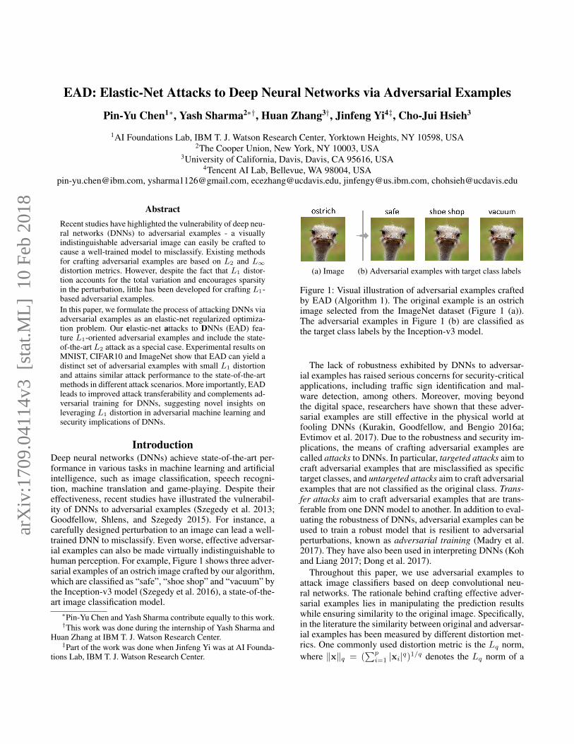
IntroductionDeep neural networks (DNNs) achieve state-of-the-art per-formance in various tasks in machine learning and artificialintelligence, such as image classification, speech recogni-tion, machine translation and game-playing. Despite theireffectiveness, recent studies have illustrated the vulnerabil-ity of DNNs to adversarial examples (Szegedy et al. 2013;Goodfellow, Shlens, and Szegedy 2015). For instance, acarefully designed perturbation to an image can lead a well-trained DNN to misclassify. Even worse, effective adversar-ial examples can also be made virtually indistinguishable tohuman perception. For example, Figure 1 shows three adver-sarial examples of an ostrich image crafted by our algorithm,which are classified as “safe”, “shoe shop” and “vacuum” bythe Inception-v3 model (Szegedy et al. 2016), a state-of-the-art image classification model.∗Pin-Yu Chen and Yash Sharma contribute equally to this work.†This work was done during the internship of Yash Sharma and

Huan Zhang at IBM T. J. Watson Research Center.‡Part of the work was done when Jinfeng Yi was at AI Founda-

tions Lab, IBM T. J. Watson Research Center.

(a) Image (b) Adversarial examples with target class labels

Figure 1: Visual illustration of adversarial examples craftedby EAD (Algorithm 1). The original example is an ostrichimage selected from the ImageNet dataset (Figure 1 (a)).The adversarial examples in Figure 1 (b) are classified asthe target class labels by the Inception-v3 model.

The lack of robustness exhibited by DNNs to adversar-ial examples has raised serious concerns for security-criticalapplications, including traffic sign identification and mal-ware detection, among others. Moreover, moving beyondthe digital space, researchers have shown that these adver-sarial examples are still effective in the physical world atfooling DNNs (Kurakin, Goodfellow, and Bengio 2016a;Evtimov et al. 2017). Due to the robustness and security im-plications, the means of crafting adversarial examples arecalled attacks to DNNs. In particular, targeted attacks aim tocraft adversarial examples that are misclassified as specifictarget classes, and untargeted attacks aim to craft adversarialexamples that are not classified as the original class. Trans-fer attacks aim to craft adversarial examples that are trans-ferable from one DNN model to another. In addition to eval-uating the robustness of DNNs, adversarial examples can beused to train a robust model that is resilient to adversarialperturbations, known as adversarial training (Madry et al.2017). They have also been used in interpreting DNNs (Kohand Liang 2017; Dong et al. 2017).

Throughout this paper, we use adversarial examples toattack image classifiers based on deep convolutional neu-ral networks. The rationale behind crafting effective adver-sarial examples lies in manipulating the prediction resultswhile ensuring similarity to the original image. Specifically,in the literature the similarity between original and adversar-ial examples has been measured by different distortion met-rics. One commonly used distortion metric is the Lq norm,where ‖x‖q = (

∑pi=1 |xi|q)1/q denotes the Lq norm of a

arX

iv:1

709.

0411

4v3

[st

at.M

L]

10

Feb

2018

p-dimensional vector x = [x1, . . . ,xp] for any q ≥ 1. Inparticular, when crafting adversarial examples, the L∞ dis-tortion metric is used to evaluate the maximum variationin pixel value changes (Goodfellow, Shlens, and Szegedy2015), while the L2 distortion metric is used to improve thevisual quality (Carlini and Wagner 2017b). However, despitethe fact that the L1 norm is widely used in problems relatedto image denoising and restoration (Fu et al. 2006), as wellas sparse recovery (Candes and Wakin 2008), L1-based ad-versarial examples have not been rigorously explored. In thecontext of adversarial examples, L1 distortion accounts forthe total variation in the perturbation and serves as a popularconvex surrogate function of the L0 metric, which measuresthe number of modified pixels (i.e., sparsity) by the pertur-bation. To bridge this gap, we propose an attack algorithmbased on elastic-net regularization, which we call elastic-net attacks to DNNs (EAD). Elastic-net regularization is alinear mixture of L1 and L2 penalty functions, and it hasbeen a standard tool for high-dimensional feature selectionproblems (Zou and Hastie 2005). In the context of attackingDNNs, EAD opens up new research directions since it gen-eralizes the state-of-the-art attack proposed in (Carlini andWagner 2017b) based on L2 distortion, and is able to craftL1-oriented adversarial examples that are more effective andfundamentally different from existing attack methods.

To explore the utility of L1-based adversarial exam-ples crafted by EAD, we conduct extensive experiments onMNIST, CIFAR10 and ImageNet in different attack scenar-ios. Compared to the state-of-the-art L2 and L∞ attacks(Kurakin, Goodfellow, and Bengio 2016b; Carlini and Wag-ner 2017b), EAD can attain similar attack success rate whenbreaking undefended and defensively distilled DNNs (Pa-pernot et al. 2016b). More importantly, we find that L1 at-tacks attain superior performance over L2 and L∞ attacksin transfer attacks and complement adversarial training. Forthe most difficult dataset (MNIST), EAD results in improvedattack transferability from an undefended DNN to a defen-sively distilled DNN, achieving nearly 99% attack successrate. In addition, joint adversarial training with L1 and L2

based examples can further enhance the resilience of DNNsto adversarial perturbations. These results suggest that EADyields a distinct, yet more effective, set of adversarial ex-amples. Moreover, evaluating attacks based on L1 distor-tion provides novel insights on adversarial machine learningand security implications of DNNs, suggesting that L1 maycomplement L2 and L∞ based examples toward furtheringa thorough adversarial machine learning framework.

Related WorkHere we summarize related works on attacking and defend-ing DNNs against adversarial examples.

Attacks to DNNsFGM and I-FGM: Let x0 and x denote the original and ad-versarial examples, respectively, and let t denote the targetclass to attack. Fast gradient methods (FGM) use the gradi-ent ∇J of the training loss J with respect to x0 for craft-ing adversarial examples (Goodfellow, Shlens, and Szegedy

2015). For L∞ attacks, x is crafted by

x = x0 − ε · sign(∇J(x0, t)), (1)

where ε specifies the L∞ distortion between x and x0, andsign(∇J) takes the sign of the gradient. For L1 and L2 at-tacks, x is crafted by

x = x0 − ε∇J(x0, t)

‖∇J(x0, t)‖q(2)

for q = 1, 2, where ε specifies the corresponding distortion.Iterative fast gradient methods (I-FGM) were proposed in(Kurakin, Goodfellow, and Bengio 2016b), which iterativelyuse FGM with a finer distortion, followed by an ε-ball clip-ping. Untargeted attacks using FGM and I-FGM can be im-plemented in a similar fashion.C&W attack: Instead of leveraging the training loss, Carliniand Wagner designed an L2-regularized loss function basedon the logit layer representation in DNNs for crafting adver-sarial examples (Carlini and Wagner 2017b). Its formulationturns out to be a special case of our EAD formulation, whichwill be discussed in the following section. The C&W attackis considered to be one of the strongest attacks to DNNs, as itcan successfully break undefended and defensively distilledDNNs and can attain remarkable attack transferability.JSMA: Papernot et al. proposed a Jacobian-based saliencymap algorithm (JSMA) for characterizing the input-outputrelation of DNNs (Papernot et al. 2016a). It can be viewed asa greedy attack algorithm that iteratively modifies the mostinfluential pixel for crafting adversarial examples.DeepFool: DeepFool is an untargeted L2 attack algorithm(Moosavi-Dezfooli, Fawzi, and Frossard 2016) based on thetheory of projection to the closest separating hyperplane inclassification. It is also used to craft a universal perturba-tion to mislead DNNs trained on natural images (Moosavi-Dezfooli et al. 2016).Black-box attacks: Crafting adversarial examples in theblack-box case is plausible if one allows querying of the tar-get DNN. In (Papernot et al. 2017), JSMA is used to traina substitute model for transfer attacks. In (?), an effectiveblack-box C&W attack is made possible using zeroth orderoptimization (ZOO). In the more stringent attack scenariowhere querying is prohibited, ensemble methods can be usedfor transfer attacks (Liu et al. 2016).

Defenses in DNNsDefensive distillation: Defensive distillation (Papernot et al.2016b) defends against adversarial perturbations by usingthe distillation technique in (Hinton, Vinyals, and Dean2015) to retrain the same network with class probabilitiespredicted by the original network. It also introduces the tem-perature parameter T in the softmax layer to enhance therobustness to adversarial perturbations.Adversarial training: Adversarial training can be imple-mented in a few different ways. A standard approach isaugmenting the original training dataset with the label-corrected adversarial examples to retrain the network. Mod-ifying the training loss or the network architecture to in-crease the robustness of DNNs to adversarial examples has

been proposed in (Zheng et al. 2016; Madry et al. 2017;Tramer et al. 2017; Zantedeschi, Nicolae, and Rawat 2017).Detection methods: Detection methods utilize statisticaltests to differentiate adversarial from benign examples(Feinman et al. 2017; Grosse et al. 2017; Lu, Issaranon, andForsyth 2017; Xu, Evans, and Qi 2017). However, 10 differ-ent detection methods were unable to detect the C&W attack(Carlini and Wagner 2017a).

EAD: Elastic-Net Attacks to DNNsPreliminaries on Elastic-Net RegularizationElastic-net regularization is a widely used technique in solv-ing high-dimensional feature selection problems (Zou andHastie 2005). It can be viewed as a regularizer that lin-early combines L1 and L2 penalty functions. In general,elastic-net regularization is used in the following minimiza-tion problem:

minimizez∈Z f(z) + λ1‖z‖1 + λ2‖z‖22, (3)

where z is a vector of p optimization variables, Z indicatesthe set of feasible solutions, f(z) denotes a loss function,‖z‖q denotes the Lq norm of z, and λ1, λ2 ≥ 0 are theL1 and L2 regularization parameters, respectively. The termλ1‖z‖1+λ2‖z‖22 in (3) is called the elastic-net regularizer ofz. For standard regression problems, the loss function f(z)is the mean squared error, the vector z represents the weights(coefficients) on the features, and the set Z = Rp. In partic-ular, the elastic-net regularization in (3) degenerates to theLASSO formulation when λ2 = 0, and becomes the ridgeregression formulation when λ1 = 0. It is shown in (Zouand Hastie 2005) that elastic-net regularization is able to se-lect a group of highly correlated features, which overcomesthe shortcoming of high-dimensional feature selection whensolely using the LASSO or ridge regression techniques.

EAD Formulation and GeneralizationInspired by the C&W attack (Carlini and Wagner 2017b),we adopt the same loss function f for crafting adversarialexamples. Specifically, given an image x0 and its correct la-bel denoted by t0, let x denote the adversarial example ofx0 with a target class t 6= t0. The loss function f(x) fortargeted attacks is defined as

f(x, t) = max{maxj 6=t

[Logit(x)]j − [Logit(x)]t,−κ}, (4)

where Logit(x) = [[Logit(x)]1, . . . , [Logit(x)]K ] ∈ RKis the logit layer (the layer prior to the softmax layer) rep-resentation of x in the considered DNN, K is the num-ber of classes for classification, and κ ≥ 0 is a confi-dence parameter that guarantees a constant gap betweenmaxj 6=t[Logit(x)]j and [Logit(x)]t.

It is worth noting that the term [Logit(x)]t is proportionalto the probability of predicting x as label t, since by thesoftmax classification rule,

Prob(Label(x) = t) =exp([Logit(x)]t)∑Kj=1 exp([Logit(x)]j)

. (5)

Consequently, the loss function in (4) aims to render the la-bel t the most probable class for x, and the parameter κcontrols the separation between t and the next most likelyprediction among all classes other than t. For untargeted at-tacks, the loss function in (4) can be modified asf(x) = max{[Logit(x)]t0 −max

j 6=t0[Logit(x)]j ,−κ}. (6)

In this paper, we focus on targeted attacks since they aremore challenging than untargeted attacks. Our EAD algo-rithm (Algorithm 1) can directly be applied to untargetedattacks by replacing f(x, t) in (4) with f(x) in (6).

In addition to manipulating the prediction via the lossfunction in (4), introducing elastic-net regularization furtherencourages similarity to the original image when craftingadversarial examples. Our formulation of elastic-net attacksto DNNs (EAD) for crafting an adversarial example (x, t)with respect to a labeled natural image (x0, t0) is as follows:

minimizex c · f(x, t) + β‖x− x0‖1 + ‖x− x0‖22subject to x ∈ [0, 1]p, (7)

where f(x, t) is as defined in (4), c, β ≥ 0 are the regular-ization parameters of the loss function f and the L1 penalty,respectively. The box constraint x ∈ [0, 1]p restricts x to aproperly scaled image space, which can be easily satisfied bydividing each pixel value by the maximum attainable value(e.g., 255). Upon defining the perturbation of x relative to x0

as δ = x−x0, the EAD formulation in (7) aims to find an ad-versarial example x that will be classified as the target classt while minimizing the distortion in δ in terms of the elastic-net loss β‖δ‖1 + ‖δ‖22, which is a linear combination of L1

and L2 distortion metrics between x and x0. Notably, theformulation of the C&W attack (Carlini and Wagner 2017b)becomes a special case of the EAD formulation in (7) whenβ = 0, which disregards the L1 penalty on δ. However, theL1 penalty is an intuitive regularizer for crafting adversarialexamples, as ‖δ‖1 =

∑pi=1 |δi| represents the total varia-

tion of the perturbation, and is also a widely used surrogatefunction for promoting sparsity in the perturbation. As willbe evident in the performance evaluation section, includingthe L1 penalty for the perturbation indeed yields a distinctset of adversarial examples, and it leads to improved attacktransferability and complements adversarial learning.

EAD AlgorithmWhen solving the EAD formulation in (7) without the L1

penalty (i.e., β = 0), Carlini and Wagner used a change-of-variable (COV) approach via the tanh transformation onx in order to remove the box constraint x ∈ [0, 1]p (Car-lini and Wagner 2017b). When β > 0, we find that the sameCOV approach is not effective in solving (7), since the corre-sponding adversarial examples are insensitive to the changesin β (see the performance evaluation section for details).Since the L1 penalty is a non-differentiable, yet piece-wiselinear, function, the failure of the COV approach in solving(7) can be explained by its inefficiency in subgradient-basedoptimization problems (Duchi and Singer 2009).

To efficiently solve the EAD formulation in (7) forcrafting adversarial examples, we propose to use the iter-ative shrinkage-thresholding algorithm (ISTA) (Beck and

Teboulle 2009). ISTA can be viewed as a regular first-order optimization algorithm with an additional shrinkage-thresholding step on each iteration. In particular, let g(x) =c·f(x)+‖x−x0‖22 and let∇g(x) be the numerical gradientof g(x) computed by the DNN. At the k+ 1-th iteration, theadversarial example x(k+1) of x0 is computed by

x(k+1) = Sβ(x(k) − αk∇g(x(k))), (8)where αk denotes the step size at the k + 1-th iteration, andSβ : Rp 7→ Rp is an element-wise projected shrinkage-thresholding function, which is defined as

[Sβ(z)]i =

{min{zi − β, 1}, if zi − x0i > β;x0i, if |zi − x0i| ≤ β;max{zi + β, 0}, if zi − x0i < −β,

(9)for any i ∈ {1, . . . , p}. If |zi − x0i| > β, it shrinks theelement zi by β and projects the resulting element to thefeasible box constraint between 0 and 1. On the other hand,if |zi − x0i| ≤ β, it thresholds zi by setting [Sβ(z)]i = x0i.The proof of optimality of using (8) for solving the EADformulation in (7) is given in the supplementary material1.Notably, since g(x) is the attack objective function of theC&W method (Carlini and Wagner 2017b), the ISTA oper-ation in (8) can be viewed as a robust version of the C&Wmethod that shrinks a pixel value of the adversarial exampleif the deviation to the original image is greater than β, andkeeps a pixel value unchanged if the deviation is less than β.

Our EAD algorithm for crafting adversarial examples issummarized in Algorithm 1. For computational efficiency, afast ISTA (FISTA) for EAD is implemented, which yieldsthe optimal convergence rate for first-order optimizationmethods (Beck and Teboulle 2009). The slack vector y(k)

in Algorithm 1 incorporates the momentum in x(k) for ac-celeration. In the experiments, we set the initial learning rateα0 = 0.01 with a square-root decay factor in k. During theEAD iterations, the iterate x(k) is considered as a success-ful adversarial example of x0 if the model predicts its mostlikely class to be the target class t. The final adversarial ex-ample x is selected from all successful examples based ondistortion metrics. In this paper we consider two decisionrules for selecting x: the least elastic-net (EN) and L1 dis-tortions relative to x0. The influence of β, κ and the decisionrules on EAD will be investigated in the following section.

Performance EvaluationIn this section, we compare the proposed EAD with thestate-of-the-art attacks to DNNs on three image classifica-tion datasets - MNIST, CIFAR10 and ImageNet. We wouldlike to show that (i) EAD can attain attack performance sim-ilar to the C&W attack in breaking undefended and defen-sively distilled DNNs, since the C&W attack is a specialcase of EAD when β = 0; (ii) Comparing to existing L1-based FGM and I-FGM methods, the adversarial examplesusing EAD can lead to significantly lower L1 distortion andbetter attack success rate; (iii) The L1-based adversarial ex-amples crafted by EAD can achieve improved attack trans-ferability and complement adversarial training.

1https://arxiv.org/abs/1709.04114

Algorithm 1 Elastic-Net Attacks to DNNs (EAD)

Input: original labeled image (x0, t0), target attack classt, attack transferability parameter κ, L1 regularization pa-rameter β, step size αk, # of iterations IOutput: adversarial example xInitialization: x(0) = y(0) = x0

for k = 0 to I − 1 dox(k+1) = Sβ(y(k) − αk∇g(y(k)))

y(k+1) = x(k+1) + kk+3 (x(k+1) − x(k))

end forDecision rule: determine x from successful examples in{x(k)}Ik=1 (EN rule or L1 rule).

Comparative MethodsWe compare EAD with the following targeted attacks, whichare the most effective methods for crafting adversarial exam-ples in different distortion metrics.C&W attack: The state-of-the-art L2 targeted attack pro-posed by Carlini and Wagner (Carlini and Wagner 2017b),which is a special case of EAD when β = 0.FGM: The fast gradient method proposed in (Goodfellow,Shlens, and Szegedy 2015). The FGM attacks using differ-ent distortion metrics are denoted by FGM-L1, FGM-L2 andFGM-L∞.I-FGM: The iterative fast gradient method proposed in (Ku-rakin, Goodfellow, and Bengio 2016b). The I-FGM attacksusing different distortion metrics are denoted by I-FGM-L1,I-FGM-L2 and I-FGM-L∞.

Experiment Setup and Parameter SettingOur experiment setup is based on Carlini and Wagner’sframework2. For both the EAD and C&W attacks, we use thedefault setting1, which implements 9 binary search steps onthe regularization parameter c (starting from 0.001) and runsI = 1000 iterations for each step with the initial learningrate α0 = 0.01. For finding successful adversarial examples,we use the reference optimizer1 (ADAM) for the C&W at-tack and implement the projected FISTA (Algorithm 1) withthe square-root decaying learning rate for EAD. Similar tothe C&W attack, the final adversarial example of EAD is se-lected by the least distorted example among all the success-ful examples. The sensitivity analysis of the L1 parameter βand the effect of the decision rule on EAD will be investi-gated in the forthcoming paragraph. Unless specified, we setthe attack transferability parameter κ = 0 for both attacks.

We implemented FGM and I-FGM using the CleverHanspackage3. The best distortion parameter ε is determined bya fine-grained grid search - for each image, the smallest εin the grid leading to a successful attack is reported. ForI-FGM, we perform 10 FGM iterations (the default value)with ε-ball clipping. The distortion parameter ε′ in eachFGM iteration is set to be ε/10, which has been shown tobe an effective attack setting in (Tramer et al. 2017). The

2https://github.com/carlini/nn robust attacks3https://github.com/tensorflow/cleverhans

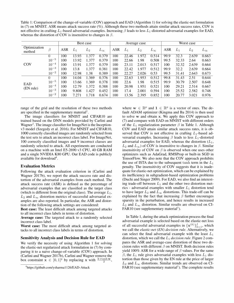
Table 1: Comparison of the change-of-variable (COV) approach and EAD (Algorithm 1) for solving the elastic-net formulationin (7) on MNIST. ASR means attack success rate (%). Although these two methods attain similar attack success rates, COV isnot effective in crafting L1-based adversarial examples. Increasing β leads to less L1-distorted adversarial examples for EAD,whereas the distortion of COV is insensitive to changes in β.

Best case Average case Worst caseOptimizationmethod β ASR L1 L2 L∞ ASR L1 L2 L∞ ASR L1 L2 L∞

COV

0 100 13.93 1.377 0.379 100 22.46 1.972 0.514 99.9 32.3 2.639 0.66310−5 100 13.92 1.377 0.379 100 22.66 1.98 0.508 99.5 32.33 2.64 0.66310−4 100 13.91 1.377 0.379 100 23.11 2.013 0.517 100 32.32 2.639 0.66410−3 100 13.8 1.377 0.381 100 22.42 1.977 0.512 99.9 32.2 2.639 0.66410−2 100 12.98 1.38 0.389 100 22.27 2.026 0.53 99.5 31.41 2.643 0.673

EAD(EN rule)

0 100 14.04 1.369 0.376 100 22.63 1.953 0.512 99.8 31.43 2.51 0.64410−5 100 13.66 1.369 0.378 100 22.6 1.98 0.515 99.9 30.79 2.507 0.64810−4 100 12.79 1.372 0.388 100 20.98 1.951 0.521 100 29.21 2.514 0.66710−3 100 9.808 1.427 0.452 100 17.4 2.001 0.594 100 25.52 2.582 0.74810−2 100 7.271 1.718 0.674 100 13.56 2.395 0.852 100 20.77 3.021 0.976

range of the grid and the resolution of these two methodsare specified in the supplementary material1.

The image classifiers for MNIST and CIFAR10 aretrained based on the DNN models provided by Carlini andWagner1. The image classifier for ImageNet is the Inception-v3 model (Szegedy et al. 2016). For MNIST and CIFAR10,1000 correctly classified images are randomly selected fromthe test sets to attack an incorrect class label. For ImageNet,100 correctly classified images and 9 incorrect classes arerandomly selected to attack. All experiments are conductedon a machine with an Intel E5-2690 v3 CPU, 40 GB RAMand a single NVIDIA K80 GPU. Our EAD code is publiclyavailable for download4.

Evaluation MetricsFollowing the attack evaluation criterion in (Carlini andWagner 2017b), we report the attack success rate and dis-tortion of the adversarial examples from each method. Theattack success rate (ASR) is defined as the percentage ofadversarial examples that are classified as the target class(which is different from the original class). The average L1,L2 and L∞ distortion metrics of successful adversarial ex-amples are also reported. In particular, the ASR and distor-tion of the following attack settings are considered:Best case: The least difficult attack among targeted attacksto all incorrect class labels in terms of distortion.Average case: The targeted attack to a randomly selectedincorrect class label.Worst case: The most difficult attack among targeted at-tacks to all incorrect class labels in terms of distortion.

Sensitivity Analysis and Decision Rule for EADWe verify the necessity of using Algorithm 1 for solvingthe elastic-net regularized attack formulation in (7) by com-paring it to a naive change-of-variable (COV) approach. In(Carlini and Wagner 2017b), Carlini and Wagner remove thebox constraint x ∈ [0, 1]p by replacing x with 1+tanhw

2 ,

4https://github.com/ysharma1126/EAD-Attack

where w ∈ Rp and 1 ∈ Rp is a vector of ones. The de-fault ADAM optimizer (Kingma and Ba 2014) is then usedto solve w and obtain x. We apply this COV approach to(7) and compare with EAD on MNIST with different ordersof the L1 regularization parameter β in Table 1. AlthoughCOV and EAD attain similar attack success rates, it is ob-served that COV is not effective in crafting L1-based ad-versarial examples. Increasing β leads to less L1-distortedadversarial examples for EAD, whereas the distortion (L1,L2 and L∞) of COV is insensitive to changes in β. Similarinsensitivity of COV on β is observed when one uses otheroptimizers such as AdaGrad, RMSProp or built-in SGD inTensorFlow. We also note that the COV approach prohibitsthe use of ISTA due to the subsequent tanh term in the L1

penalty. The insensitivity of COV suggests that it is inade-quate for elastic-net optimization, which can be explained byits inefficiency in subgradient-based optimization problems(Duchi and Singer 2009). For EAD, we also find an interest-ing trade-off between L1 and the other two distortion met-rics - adversarial examples with smaller L1 distortion tendto have larger L2 and L∞ distortions. This trade-off can beexplained by the fact that increasing β further encouragessparsity in the perturbation, and hence results in increasedL2 and L∞ distortion. Similar results are observed on CI-FAR10 (see supplementary material1).

In Table 1, during the attack optimization process the finaladversarial example is selected based on the elastic-net lossof all successful adversarial examples in {x(k)}Ik=1, whichwe call the elastic-net (EN) decision rule. Alternatively, wecan select the final adversarial example with the least L1

distortion, which we call the L1 decision rule. Figure 2 com-pares the ASR and average-case distortion of these two de-cision rules with different β on MNIST. Both decision rulesyield 100% ASR for a wide range of β values. For the sameβ, the L1 rule gives adversarial examples with less L1 dis-tortion than those given by the EN rule at the price of largerL2 and L∞ distortions. Similar trends are observed on CI-FAR10 (see supplementary material1). The complete results

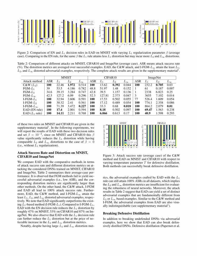
Figure 2: Comparison of EN and L1 decision rules in EAD on MNIST with varying L1 regularization parameter β (averagecase). Comparing to the EN rule, for the same β the L1 rule attains less L1 distortion but may incur more L2 and L∞ distortions.

Table 2: Comparison of different attacks on MNIST, CIFAR10 and ImageNet (average case). ASR means attack success rate(%). The distortion metrics are averaged over successful examples. EAD, the C&W attack, and I-FGM-L∞ attain the least L1,L2, and L∞ distorted adversarial examples, respectively. The complete attack results are given in the supplementary material1.

MNIST CIFAR10 ImageNetAttack method ASR L1 L2 L∞ ASR L1 L2 L∞ ASR L1 L2 L∞C&W (L2) 100 22.46 1.972 0.514 100 13.62 0.392 0.044 100 232.2 0.705 0.03FGM-L1 39 53.5 4.186 0.782 48.8 51.97 1.48 0.152 1 61 0.187 0.007FGM-L2 34.6 39.15 3.284 0.747 42.8 39.5 1.157 0.136 1 2338 6.823 0.25FGM-L∞ 42.5 127.2 6.09 0.296 52.3 127.81 2.373 0.047 3 3655 7.102 0.014I-FGM-L1 100 32.94 2.606 0.591 100 17.53 0.502 0.055 77 526.4 1.609 0.054I-FGM-L2 100 30.32 2.41 0.561 100 17.12 0.489 0.054 100 774.1 2.358 0.086I-FGM-L∞ 100 71.39 3.472 0.227 100 33.3 0.68 0.018 100 864.2 2.079 0.01EAD (EN rule) 100 17.4 2.001 0.594 100 8.18 0.502 0.097 100 69.47 1.563 0.238EAD (L1 rule) 100 14.11 2.211 0.768 100 6.066 0.613 0.17 100 40.9 1.598 0.293

of these two rules on MNIST and CIFAR10 are given in thesupplementary material1. In the following experiments, wewill report the results of EAD with these two decision rulesand set β = 10−3, since on MNIST and CIFAR10 this βvalue significantly reduces the L1 distortion while havingcomparable L2 and L∞ distortions to the case of β = 0(i.e., without L1 regularization).

Attack Success Rate and Distortion on MNIST,CIFAR10 and ImageNetWe compare EAD with the comparative methods in termsof attack success rate and different distortion metrics on at-tacking the considered DNNs trained on MNIST, CIFAR10and ImageNet. Table 2 summarizes their average-case per-formance. It is observed that FGM methods fail to yield suc-cessful adversarial examples (i.e., low ASR), and the cor-responding distortion metrics are significantly larger thanother methods. On the other hand, the C&W attack, I-FGMand EAD all lead to 100% attack success rate. Further-more, EAD, the C&W method, and I-FGM-L∞ attain theleastL1,L2, andL∞ distorted adversarial examples, respec-tively. We note that EAD significantly outperforms the exist-ingL1-based method (I-FGM-L1). Compared to I-FGM-L1,EAD with the EN decision rule reduces the L1 distortion byroughly 47% on MNIST, 53% on CIFAR10 and 87% on Im-ageNet. We also observe that EAD with the L1 decision rulecan further reduce the L1 distortion but at the price of no-ticeable increase in the L2 and L∞ distortion metrics.

Notably, despite having large L2 and L∞ distortion met-

Figure 3: Attack success rate (average case) of the C&Wmethod and EAD on MNIST and CIFAR10 with respect tovarying temperature parameter T for defensive distillation.Both methods can successfully break defensive distillation.

rics, the adversarial examples crafted by EAD with the L1

rule can still attain 100% ASRs in all datasets, which impliestheL2 andL∞ distortion metrics are insufficient for evaluat-ing the robustness of neural networks. Moreover, the attackresults in Table 2 suggest that EAD can yield a set of distinctadversarial examples that are fundamentally different fromL2 or L∞ based examples. Similar to the C&W method andI-FGM, the adversarial examples from EAD are also visu-ally indistinguishable (see supplementary material1).

Breaking Defensive DistillationIn addition to breaking undefended DNNs via adversarialexamples, here we show that EAD can also break defen-sively distilled DNNs. Defensive distillation (Papernot et al.

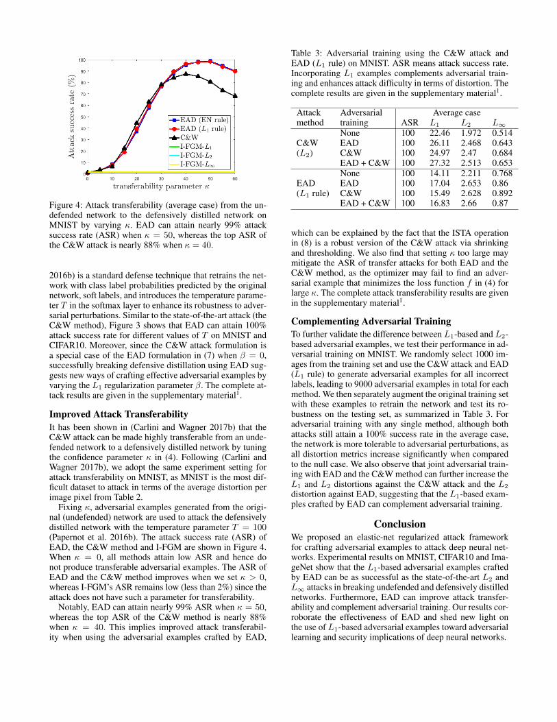
Figure 4: Attack transferability (average case) from the un-defended network to the defensively distilled network onMNIST by varying κ. EAD can attain nearly 99% attacksuccess rate (ASR) when κ = 50, whereas the top ASR ofthe C&W attack is nearly 88% when κ = 40.

2016b) is a standard defense technique that retrains the net-work with class label probabilities predicted by the originalnetwork, soft labels, and introduces the temperature parame-ter T in the softmax layer to enhance its robustness to adver-sarial perturbations. Similar to the state-of-the-art attack (theC&W method), Figure 3 shows that EAD can attain 100%attack success rate for different values of T on MNIST andCIFAR10. Moreover, since the C&W attack formulation isa special case of the EAD formulation in (7) when β = 0,successfully breaking defensive distillation using EAD sug-gests new ways of crafting effective adversarial examples byvarying the L1 regularization parameter β. The complete at-tack results are given in the supplementary material1.

Improved Attack TransferabilityIt has been shown in (Carlini and Wagner 2017b) that theC&W attack can be made highly transferable from an unde-fended network to a defensively distilled network by tuningthe confidence parameter κ in (4). Following (Carlini andWagner 2017b), we adopt the same experiment setting forattack transferability on MNIST, as MNIST is the most dif-ficult dataset to attack in terms of the average distortion perimage pixel from Table 2.

Fixing κ, adversarial examples generated from the origi-nal (undefended) network are used to attack the defensivelydistilled network with the temperature parameter T = 100(Papernot et al. 2016b). The attack success rate (ASR) ofEAD, the C&W method and I-FGM are shown in Figure 4.When κ = 0, all methods attain low ASR and hence donot produce transferable adversarial examples. The ASR ofEAD and the C&W method improves when we set κ > 0,whereas I-FGM’s ASR remains low (less than 2%) since theattack does not have such a parameter for transferability.

Notably, EAD can attain nearly 99% ASR when κ = 50,whereas the top ASR of the C&W method is nearly 88%when κ = 40. This implies improved attack transferabil-ity when using the adversarial examples crafted by EAD,

Table 3: Adversarial training using the C&W attack andEAD (L1 rule) on MNIST. ASR means attack success rate.Incorporating L1 examples complements adversarial train-ing and enhances attack difficulty in terms of distortion. Thecomplete results are given in the supplementary material1.

Attackmethod

Adversarialtraining

Average caseASR L1 L2 L∞

C&W(L2)

None 100 22.46 1.972 0.514EAD 100 26.11 2.468 0.643C&W 100 24.97 2.47 0.684EAD + C&W 100 27.32 2.513 0.653

EAD(L1 rule)

None 100 14.11 2.211 0.768EAD 100 17.04 2.653 0.86C&W 100 15.49 2.628 0.892EAD + C&W 100 16.83 2.66 0.87

which can be explained by the fact that the ISTA operationin (8) is a robust version of the C&W attack via shrinkingand thresholding. We also find that setting κ too large maymitigate the ASR of transfer attacks for both EAD and theC&W method, as the optimizer may fail to find an adver-sarial example that minimizes the loss function f in (4) forlarge κ. The complete attack transferability results are givenin the supplementary material1.

Complementing Adversarial TrainingTo further validate the difference between L1-based and L2-based adversarial examples, we test their performance in ad-versarial training on MNIST. We randomly select 1000 im-ages from the training set and use the C&W attack and EAD(L1 rule) to generate adversarial examples for all incorrectlabels, leading to 9000 adversarial examples in total for eachmethod. We then separately augment the original training setwith these examples to retrain the network and test its ro-bustness on the testing set, as summarized in Table 3. Foradversarial training with any single method, although bothattacks still attain a 100% success rate in the average case,the network is more tolerable to adversarial perturbations, asall distortion metrics increase significantly when comparedto the null case. We also observe that joint adversarial train-ing with EAD and the C&W method can further increase theL1 and L2 distortions against the C&W attack and the L2

distortion against EAD, suggesting that the L1-based exam-ples crafted by EAD can complement adversarial training.

ConclusionWe proposed an elastic-net regularized attack frameworkfor crafting adversarial examples to attack deep neural net-works. Experimental results on MNIST, CIFAR10 and Ima-geNet show that the L1-based adversarial examples craftedby EAD can be as successful as the state-of-the-art L2 andL∞ attacks in breaking undefended and defensively distillednetworks. Furthermore, EAD can improve attack transfer-ability and complement adversarial training. Our results cor-roborate the effectiveness of EAD and shed new light onthe use of L1-based adversarial examples toward adversariallearning and security implications of deep neural networks.

Acknowledgment Cho-Jui Hsieh and Huan Zhang ac-knowledge the support of NSF via IIS-1719097.

ReferencesBeck, A., and Teboulle, M. 2009. A fast iterative shrinkage-thresholding algorithm for linear inverse problems. SIAMjournal on imaging sciences 2(1):183–202.Candes, E. J., and Wakin, M. B. 2008. An introduction tocompressive sampling. IEEE signal processing magazine25(2):21–30.Carlini, N., and Wagner, D. 2017a. Adversarial examples arenot easily detected: Bypassing ten detection methods. arXivpreprint arXiv:1705.07263.Carlini, N., and Wagner, D. 2017b. Towards evaluating therobustness of neural networks. In IEEE Symposium on Se-curity and Privacy (SP), 39–57.Dong, Y.; Su, H.; Zhu, J.; and Bao, F. 2017. Towards in-terpretable deep neural networks by leveraging adversarialexamples. arXiv preprint arXiv:1708.05493.Duchi, J., and Singer, Y. 2009. Efficient online and batchlearning using forward backward splitting. Journal of Ma-chine Learning Research 10(Dec):2899–2934.Evtimov, I.; Eykholt, K.; Fernandes, E.; Kohno, T.; Li, B.;Prakash, A.; Rahmati, A.; and Song, D. 2017. Robustphysical-world attacks on machine learning models. arXivpreprint arXiv:1707.08945.Feinman, R.; Curtin, R. R.; Shintre, S.; and Gardner, A. B.2017. Detecting adversarial samples from artifacts. arXivpreprint arXiv:1703.00410.Fu, H.; Ng, M. K.; Nikolova, M.; and Barlow, J. L. 2006. Ef-ficient minimization methods of mixed l2-l1 and l1-l1 normsfor image restoration. SIAM Journal on scientific computing27(6):1881–1902.Goodfellow, I. J.; Shlens, J.; and Szegedy, C. 2015. Explain-ing and harnessing adversarial examples. ICLR’15; arXivpreprint arXiv:1412.6572.Grosse, K.; Manoharan, P.; Papernot, N.; Backes, M.; andMcDaniel, P. 2017. On the (statistical) detection of adver-sarial examples. arXiv preprint arXiv:1702.06280.Hinton, G.; Vinyals, O.; and Dean, J. 2015. Distill-ing the knowledge in a neural network. arXiv preprintarXiv:1503.02531.Kingma, D., and Ba, J. 2014. Adam: A method for stochasticoptimization. arXiv preprint arXiv:1412.6980.Koh, P. W., and Liang, P. 2017. Understanding black-boxpredictions via influence functions. ICML; arXiv preprintarXiv:1703.04730.Kurakin, A.; Goodfellow, I.; and Bengio, S. 2016a. Ad-versarial examples in the physical world. arXiv preprintarXiv:1607.02533.Kurakin, A.; Goodfellow, I.; and Bengio, S. 2016b. Adver-sarial machine learning at scale. ICLR’17; arXiv preprintarXiv:1611.01236.

Liu, Y.; Chen, X.; Liu, C.; and Song, D. 2016. Delv-ing into transferable adversarial examples and black-box at-tacks. arXiv preprint arXiv:1611.02770.Lu, J.; Issaranon, T.; and Forsyth, D. 2017. Safetynet: De-tecting and rejecting adversarial examples robustly. arXivpreprint arXiv:1704.00103.Madry, A.; Makelov, A.; Schmidt, L.; Tsipras, D.; andVladu, A. 2017. Towards deep learning models resistantto adversarial attacks. arXiv preprint arXiv:1706.06083.Moosavi-Dezfooli, S.-M.; Fawzi, A.; Fawzi, O.; andFrossard, P. 2016. Universal adversarial perturbations. arXivpreprint arXiv:1610.08401.Moosavi-Dezfooli, S.-M.; Fawzi, A.; and Frossard, P. 2016.Deepfool: a simple and accurate method to fool deep neuralnetworks. In Proceedings of the IEEE Conference on Com-puter Vision and Pattern Recognition, 2574–2582.Papernot, N.; McDaniel, P.; Jha, S.; Fredrikson, M.; Celik,Z. B.; and Swami, A. 2016a. The limitations of deep learn-ing in adversarial settings. In IEEE European Symposium onSecurity and Privacy (EuroS&P), 372–387.Papernot, N.; McDaniel, P.; Wu, X.; Jha, S.; and Swami, A.2016b. Distillation as a defense to adversarial perturbationsagainst deep neural networks. In IEEE Symposium on Secu-rity and Privacy (SP), 582–597.Papernot, N.; McDaniel, P.; Goodfellow, I.; Jha, S.; Celik,Z. B.; and Swami, A. 2017. Practical black-box attacksagainst machine learning. In ACM Asia Conference on Com-puter and Communications Security, 506–519.Parikh, N.; Boyd, S.; et al. 2014. Proximal algorithms. Foun-dations and Trends R© in Optimization 1(3):127–239.Szegedy, C.; Zaremba, W.; Sutskever, I.; Bruna, J.; Erhan,D.; Goodfellow, I.; and Fergus, R. 2013. Intriguing proper-ties of neural networks. arXiv preprint arXiv:1312.6199.Szegedy, C.; Vanhoucke, V.; Ioffe, S.; Shlens, J.; and Wojna,Z. 2016. Rethinking the inception architecture for computervision. In Proceedings of the IEEE Conference on ComputerVision and Pattern Recognition, 2818–2826.Tramer, F.; Kurakin, A.; Papernot, N.; Boneh, D.; and Mc-Daniel, P. 2017. Ensemble adversarial training: Attacks anddefenses. arXiv preprint arXiv:1705.07204.Xu, W.; Evans, D.; and Qi, Y. 2017. Feature squeezing: De-tecting adversarial examples in deep neural networks. arXivpreprint arXiv:1704.01155.Zantedeschi, V.; Nicolae, M.-I.; and Rawat, A. 2017. Ef-ficient defenses against adversarial attacks. arXiv preprintarXiv:1707.06728.Zheng, S.; Song, Y.; Leung, T.; and Goodfellow, I. 2016.Improving the robustness of deep neural networks via sta-bility training. In Proceedings of the IEEE Conference onComputer Vision and Pattern Recognition, 4480–4488.Zou, H., and Hastie, T. 2005. Regularization and variableselection via the elastic net. Journal of the Royal StatisticalSociety: Series B (Statistical Methodology) 67(2):301–320.

Supplementary MaterialProof of Optimality of (8) for Solving EAD in (3)Since the L1 penalty β‖x − x0‖1 in (3) is a non-differentiable yet smooth function, we use the proximal gra-dient method (Parikh, Boyd, and others 2014) for solvingthe EAD formulation in (3). Define ΦZ(z) to be the indica-tor function of an interval Z such that ΦZ(z) = 0 if z ∈ Zand ΦZ(z) =∞ if z /∈ Z . Using ΦZ(z), the EAD formula-tion in (3) can be rewritten as

minimizex∈Rp g(x) + β‖x− x0‖1 + Φ[0,1]p(x), (10)

where g(x) = c ·f(x, t)+‖x−x0‖22. The proximal operatorProx(x) of β‖x− x0‖1 constrained to x ∈ [0, 1]p is

Prox(x) = arg minz∈Rp

1

2‖z− x‖22 + β‖z− x0‖1 + Φ[0,1]p(z)

= arg minz∈[0,1]p

1

2‖z− x‖22 + β‖z− x0‖1

= Sβ(x), (11)

where the mapping function Sβ is defined in (9). Con-sequently, using (11), the proximal gradient algorithm forsolving (7) is iterated by

x(k+1) = Prox(x(k) − αk∇g(x(k))) (12)

= Sβ(x(k) − αk∇g(x(k))), (13)

which completes the proof.

Grid Search for FGM and I-FGM (Table 4)To determine the optimal distortion parameter ε for FGMand I-FGM methods, we adopt a fine grid search on ε. Foreach image, the best parameter is the smallest ε in the gridleading to a successful targeted attack. If the grid search failsto find a successful adversarial example, the attack is consid-ered in vain. The selected range for grid search covers thereported distortion statistics of EAD and the C&W attack.The resolution of the grid search for FGM is selected suchthat it will generate 1000 candidates of adversarial examplesduring the grid search per input image. The resolution of thegrid search for I-FGM is selected such that it will computegradients for 10000 times in total (i.e., 1000 FGM opera-tions × 10 iterations) during the grid search per input im-age, which is more than the total number of gradients (9000)computed by EAD and the C&W attack.

Table 4: Range and resolution of grid search for finding theoptimal distortion parameter ε for FGM and I-FGM.

Grid searchMethod Range Resolution

FGM-L∞ [10−3, 1] 10−3

FGM-L1 [1, 103] 1FGM-L2 [10−2, 10] 10−2

I-FGM-L∞ [10−3, 1] 10−3

I-FGM-L1 [1, 103] 1I-FGM-L2 [10−2, 10] 10−2

Comparison of COV and EAD on CIFAR10 (Table5)Table 5 compares the attack performance of using EAD (Al-gorithm 1)) and the change-of-variable (COV) approach forsolving the elastic-net formulation in (7) on CIFAR10. Sim-ilar to the MNIST results in Table 1, although COV andEAD attain similar attack success rates, we find that COVis not effective in crafting L1-based adversarial examples.Increasing β leads to less L1-distorted adversarial examplesfor EAD, whereas the distortion (L1, L2 and L∞) of COVis insensitive to changes in β. The insensitivity of COV sug-gests that it is inadequate for elastic-net optimization, whichcan be explained by its inefficiency in subgradient-based op-timization problems (Duchi and Singer 2009).

Comparison of EN and L1 decision rules in EADon MNIST and CIFAR10 (Tables 6 and 7)Figure 5 compares the average-case distortion of these twodecision rules with different values of β on CIFAR10. Forthe same β, the L1 rule gives less L1 distorted adversarialexamples than those given by the EN rule at the price oflarger L2 and L∞ distortions. We also observe that the L1

distortion does not decrease monotonically with β. In partic-ular, large β values (e.g., β = 5·10−2) may lead to increasedL1 distortion due to excessive shrinking and thresholding.Table 6 and Table 7 displays the complete attack results ofthese two decision rules on MNIST and CIFAR10, respec-tively.

Complete Attack Results and Visual Illustration onMNIST, CIFAR10 and ImageNet (Tables 8, 9 and10 and Figures 6, 7 and 8)Tables 8, 9 and 10 summarize the complete attack resultsof all the considered attack methods on MNIST, CIFAR10and ImageNet, respectively. EAD, the C&W attack and I-FGM all lead to 100% attack success rate in the averagecase. Among the three image classification datasets, Ima-geNet is the easiest one to attack due to low distortion perimage pixel, and MNIST is the most difficult one to attack.For the purpose of visual illustration, the adversarial exam-ples of selected benign images from the test sets are dis-played in Figures 6, 7 and 8. On CIFAR10 and ImageNet,the adversarial examples are visually indistinguishable. OnMNIST, the I-FGM examples are blurrier than EAD and theC&W attack.

Complete Results on Attacking DefensiveDistillation on MNIST and CIFAR10 (Tables 11and 12)Tables 11 and 12 display the complete attack results of EADand the C&W method on breaking defensive distillation withdifferent temperature parameter T on MNIST and CIFAR10.Although defensive distillation is a standard defense tech-nique for DNNs, EAD and the C&W attack can successfullybreak defensive distillation with a wide range of temperatureparameters.

Table 5: Comparison of the change-of-variable (COV) approach and EAD (Algorithm 1) for solving the elastic-net formulationin (7) on CIFAR10. ASR means attack success rate (%). Similar to the results on MNIST in Table 1, increasing β leads to lessL1-distorted adversarial examples for EAD, whereas the distortion of COV is insensitive to changes in β.

Best case Average case Worst caseOptimizationmethod β ASR L1 L2 L∞ ASR L1 L∞ L∞ ASR L1 L2 L∞

COV

0 100 7.167 0.209 0.022 100 13.62 0.392 0.044 99.9 19.17 0.546 0.06410−5 100 7.165 0.209 0.022 100 13.43 0.386 0.044 100 19.16 0.546 0.06510−4 100 7.148 0.209 0.022 99.9 13.64 0.394 0.044 99.9 19.14 0.547 0.06410−3 100 6.961 0.211 0.023 100 13.35 0.396 0.045 100 18.7 0.547 0.06610−2 100 5.963 0.222 0.029 100 11.51 0.408 0.055 100 16.31 0.556 0.077

EAD(EN rule)

0 100 6.643 0.201 0.023 99.9 13.39 0.392 0.045 99.9 18.72 0.541 0.06410−5 100 5.967 0.201 0.025 100 12.24 0.391 0.047 99.7 17.24 0.541 0.06810−4 100 4.638 0.215 0.032 99.9 10.4 0.414 0.058 99.9 14.86 0.56 0.08110−3 100 4.014 0.261 0.047 100 8.18 0.502 0.097 100 12.11 0.69 0.14710−2 100 3.688 0.357 0.085 100 8.106 0.741 0.209 100 12.59 1.053 0.351

Figure 5: Comparison of EN and L1 decision rules in EAD on CIFAR10 with varying L1 regularization parameter β (averagecase). Comparing to the EN rule, for the same β the L1 rule attains less L1 distortion but may incur more L2 and L∞ distortions.

Complete Attack Transferability Results onMNIST (Table 13 )Table 13 summarizes the transfer attack results from an un-defended DNN to a defensively distilled DNN on MNISTusing EAD, the C&W attack and I-FGM. I-FGM methodshave poor performance in attack transferability. The aver-age attack success rate (ASR) of I-FGM is below 2%. Onthe other hand, adjusting the transferability parameter κ inEAD and the C&W attack can significantly improve ASR.Tested on a wide range of κ values, the top average-caseASR for EAD is 98.6% using the EN rule and 98.1% usingthe L1 rule. The top average-case ASR for the C&W attackis 87.4%. This improvement is significantly due to the im-provement in the worst case, where the top worst-case ASRfor EAD is 87% using the EN rule and 85.8% using the L1

rule, while the top worst-case ASR for the C&W attack is30.5%. The results suggest that L1-based adversarial exam-ples have better attack transferability.

Complete Results on Adversarial Training with L1

and L2 examples (Table 14)Table 14 displays the complete results of adversarial trainingon MNIST using the L2-based adversarial examples craftedby the C&W attack and the L1-based adversarial examplescrafted by EAD with the EN or the L1 decision rule. It canbe observed that adversarial training with any single method

can render the DNN more difficult to attack in terms of in-creased distortion metrics when compared with the null case.Notably, in the average case, joint adversarial training usingL1 and L2 examples lead to increased L1 and L2 distortionagainst the C&W attack and EAD (EN), and increased L2

distortion against EAD (L1). The results suggest that EADcan complement adversarial training toward resilient DNNs.We would like to point out that in our experiments, adversar-ial training maintains comparable test accuracy. All the ad-versarially trained DNNs in Table 14 can still attain at least99% test accuracy on MNIST.

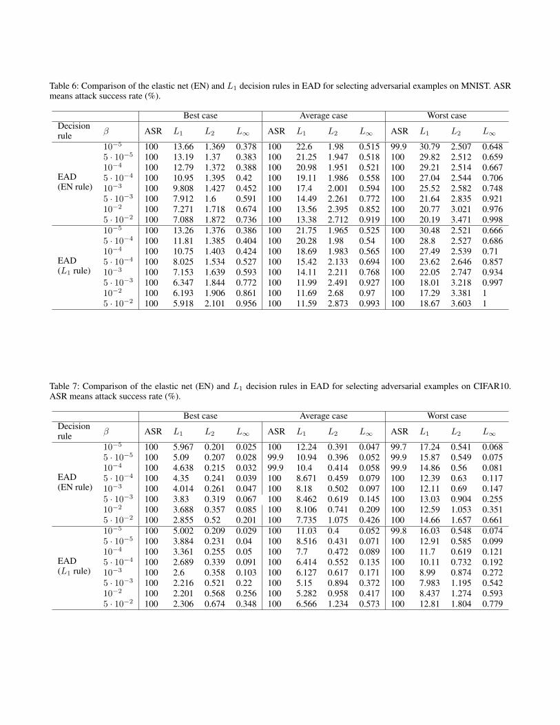
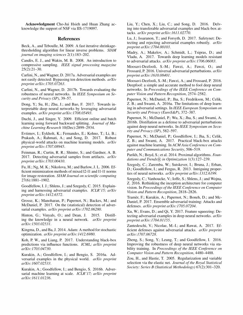
Table 6: Comparison of the elastic net (EN) and L1 decision rules in EAD for selecting adversarial examples on MNIST. ASRmeans attack success rate (%).

Best case Average case Worst caseDecisionrule β ASR L1 L2 L∞ ASR L1 L2 L∞ ASR L1 L2 L∞

EAD(EN rule)

10−5 100 13.66 1.369 0.378 100 22.6 1.98 0.515 99.9 30.79 2.507 0.6485 · 10−5 100 13.19 1.37 0.383 100 21.25 1.947 0.518 100 29.82 2.512 0.65910−4 100 12.79 1.372 0.388 100 20.98 1.951 0.521 100 29.21 2.514 0.6675 · 10−4 100 10.95 1.395 0.42 100 19.11 1.986 0.558 100 27.04 2.544 0.70610−3 100 9.808 1.427 0.452 100 17.4 2.001 0.594 100 25.52 2.582 0.7485 · 10−3 100 7.912 1.6 0.591 100 14.49 2.261 0.772 100 21.64 2.835 0.92110−2 100 7.271 1.718 0.674 100 13.56 2.395 0.852 100 20.77 3.021 0.9765 · 10−2 100 7.088 1.872 0.736 100 13.38 2.712 0.919 100 20.19 3.471 0.998

EAD(L1 rule)

10−5 100 13.26 1.376 0.386 100 21.75 1.965 0.525 100 30.48 2.521 0.6665 · 10−4 100 11.81 1.385 0.404 100 20.28 1.98 0.54 100 28.8 2.527 0.68610−4 100 10.75 1.403 0.424 100 18.69 1.983 0.565 100 27.49 2.539 0.715 · 10−4 100 8.025 1.534 0.527 100 15.42 2.133 0.694 100 23.62 2.646 0.85710−3 100 7.153 1.639 0.593 100 14.11 2.211 0.768 100 22.05 2.747 0.9345 · 10−3 100 6.347 1.844 0.772 100 11.99 2.491 0.927 100 18.01 3.218 0.99710−2 100 6.193 1.906 0.861 100 11.69 2.68 0.97 100 17.29 3.381 15 · 10−2 100 5.918 2.101 0.956 100 11.59 2.873 0.993 100 18.67 3.603 1

Table 7: Comparison of the elastic net (EN) and L1 decision rules in EAD for selecting adversarial examples on CIFAR10.ASR means attack success rate (%).

Best case Average case Worst caseDecisionrule β ASR L1 L2 L∞ ASR L1 L2 L∞ ASR L1 L2 L∞

EAD(EN rule)

10−5 100 5.967 0.201 0.025 100 12.24 0.391 0.047 99.7 17.24 0.541 0.0685 · 10−5 100 5.09 0.207 0.028 99.9 10.94 0.396 0.052 99.9 15.87 0.549 0.07510−4 100 4.638 0.215 0.032 99.9 10.4 0.414 0.058 99.9 14.86 0.56 0.0815 · 10−4 100 4.35 0.241 0.039 100 8.671 0.459 0.079 100 12.39 0.63 0.11710−3 100 4.014 0.261 0.047 100 8.18 0.502 0.097 100 12.11 0.69 0.1475 · 10−3 100 3.83 0.319 0.067 100 8.462 0.619 0.145 100 13.03 0.904 0.25510−2 100 3.688 0.357 0.085 100 8.106 0.741 0.209 100 12.59 1.053 0.3515 · 10−2 100 2.855 0.52 0.201 100 7.735 1.075 0.426 100 14.66 1.657 0.661

EAD(L1 rule)

10−5 100 5.002 0.209 0.029 100 11.03 0.4 0.052 99.8 16.03 0.548 0.0745 · 10−5 100 3.884 0.231 0.04 100 8.516 0.431 0.071 100 12.91 0.585 0.09910−4 100 3.361 0.255 0.05 100 7.7 0.472 0.089 100 11.7 0.619 0.1215 · 10−4 100 2.689 0.339 0.091 100 6.414 0.552 0.135 100 10.11 0.732 0.19210−3 100 2.6 0.358 0.103 100 6.127 0.617 0.171 100 8.99 0.874 0.2725 · 10−3 100 2.216 0.521 0.22 100 5.15 0.894 0.372 100 7.983 1.195 0.54210−2 100 2.201 0.568 0.256 100 5.282 0.958 0.417 100 8.437 1.274 0.5935 · 10−2 100 2.306 0.674 0.348 100 6.566 1.234 0.573 100 12.81 1.804 0.779

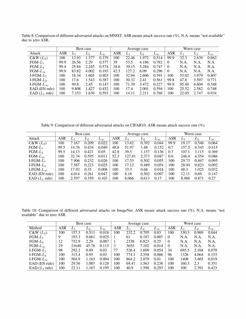
Table 8: Comparison of different adversarial attacks on MNIST. ASR means attack success rate (%). N.A. means “not available”due to zero ASR.

Best case Average case Worst caseAttack ASR L1 L2 L∞ ASR L1 L2 L∞ ASR L1 L2 L∞C&W (L2) 100 13.93 1.377 0.379 100 22.46 1.972 0.514 99.9 32.3 2.639 0.663FGM-L1 99.9 26.56 2.29 0.577 39 53.5 4.186 0.782 0 N.A. N.A. N.A.FGM-L2 99.4 25.84 2.245 0.574 34.6 39.15 3.284 0.747 0 N.A. N.A. N.A.FGM-L∞ 99.9 83.82 4.002 0.193 42.5 127.2 6.09 0.296 0 N.A. N.A. N.A.I-FGM-L1 100 18.34 1.605 0.403 100 32.94 2.606 0.591 100 53.02 3.979 0.807I-FGM-L2 100 17.6 1.543 0.387 100 30.32 2.41 0.561 99.8 47.8 3.597 0.771I-FGM-L∞ 100 49.8 2.45 0.147 100 71.39 3.472 0.227 99.9 95.48 4.604 0.348EAD (EN rule) 100 9.808 1.427 0.452 100 17.4 2.001 0.594 100 25.52 2.582 0.748EAD (L1 rule) 100 7.153 1.639 0.593 100 14.11 2.211 0.768 100 22.05 2.747 0.934

Table 9: Comparison of different adversarial attacks on CIFAR10. ASR means attack success rate (%).

Best case Average case Worst caseAttack ASR L1 L2 L∞ ASR L1 L2 L∞ ASR L1 L2 L∞C&W (L2) 100 7.167 0.209 0.022 100 13.62 0.392 0.044 99.9 19.17 0.546 0.064FGM-L1 99.5 14.76 0.434 0.049 48.8 51.97 1.48 0.152 0.7 157.5 4.345 0.415FGM-L2 99.5 14.13 0.421 0.05 42.8 39.5 1.157 0.136 0.7 107.1 3.115 0.369FGM-L∞ 100 32.74 0.595 0.011 52.3 127.81 2.373 0.047 0.6 246.4 4.554 0.086I-FGM-L1 100 7.906 0.232 0.026 100 17.53 0.502 0.055 100 29.73 0.847 0.095I-FGM-L2 100 7.587 0.223 0.025 100 17.12 0.489 0.054 100 28.94 0.823 0.092I-FGM-L∞ 100 17.92 0.35 0.008 100 33.3 0.68 0.018 100 48.3 1.025 0.032EAD (EN rule) 100 4.014 0.261 0.047 100 8.18 0.502 0.097 100 12.11 0.69 0.147EAD (L1 rule) 100 2.597 0.359 0.103 100 6.066 0.613 0.17 100 8.986 0.871 0.27

Table 10: Comparison of different adversarial attacks on ImageNet. ASR means attack success rate (%). N.A. means “notavailable” due to zero ASR.

Best case Average case Worst caseMethod ASR L1 L2 L∞ ASR L1 L2 L∞ ASR L1 L2 L∞C&W (L2) 100 157.3 0.511 0.018 100 232.2 0.705 0.03 100 330.3 0.969 0.044FGM-L1 9 193.3 0.661 0.025 1 61 0.187 0.007 0 N.A. N.A. N.A.FGM-L2 12 752.9 2.29 0.087 1 2338 6.823 0.25 0 N.A. N.A. N.A.FGM-L∞ 19 21640 45.76 0.115 3 3655 7.102 0.014 0 N.A. N.A. N.A.I-FGM-L1 98 292.2 0.89 0.03 77 526.4 1.609 0.054 34 695.5 2.104 0.078I-FGM-L2 100 315.4 0.95 0.03 100 774.1 2.358 0.086 96 1326 4.064 0.153I-FGM-L∞ 100 504.9 1.163 0.004 100 864.2 2.079 0.01 100 1408 3.465 0.019EAD (EN rule) 100 29.56 1.007 0.128 100 69.47 1.563 0.238 100 160.3 2.3 0.351EAD (L1 rule) 100 22.11 1.167 0.195 100 40.9 1.598 0.293 100 100 2.391 0.423

(a) EAD (EN rule) (b) EAD (L1 rule) (c) I-FGM-L1

(d) I-FGM-L2 (e) I-FGM-L∞ (f) C&W

Figure 6: Visual illustration of adversarial examples crafted by different attack methods on MNIST. For each method, the imagesdisplayed on the diagonal are the original examples. In each row, the off-diagonal images are the corresponding adversarialexamples with columns indexing target labels (from left to right: digits 0 to 9).

(a) EAD (EN rule) (b) EAD (L1 rule) (c) I-FGM-L1

(d) I-FGM-L2 (e) I-FGM-L∞ (f) C&W

Figure 7: Visual illustration of adversarial examples crafted by different attack methods on CIFAR10. For each method, the im-ages displayed on the diagonal are the original examples. In each row, the off-diagonal images are the corresponding adversarialexamples with columns indexing target labels.

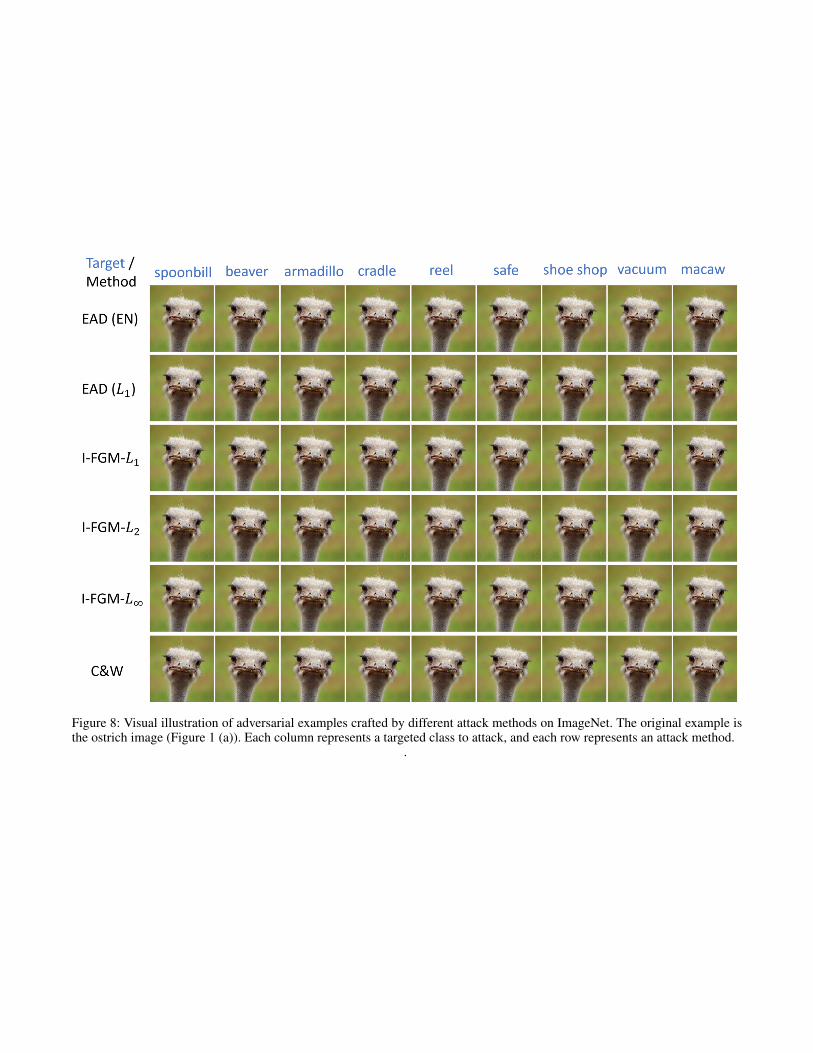
Figure 8: Visual illustration of adversarial examples crafted by different attack methods on ImageNet. The original example isthe ostrich image (Figure 1 (a)). Each column represents a targeted class to attack, and each row represents an attack method.

.

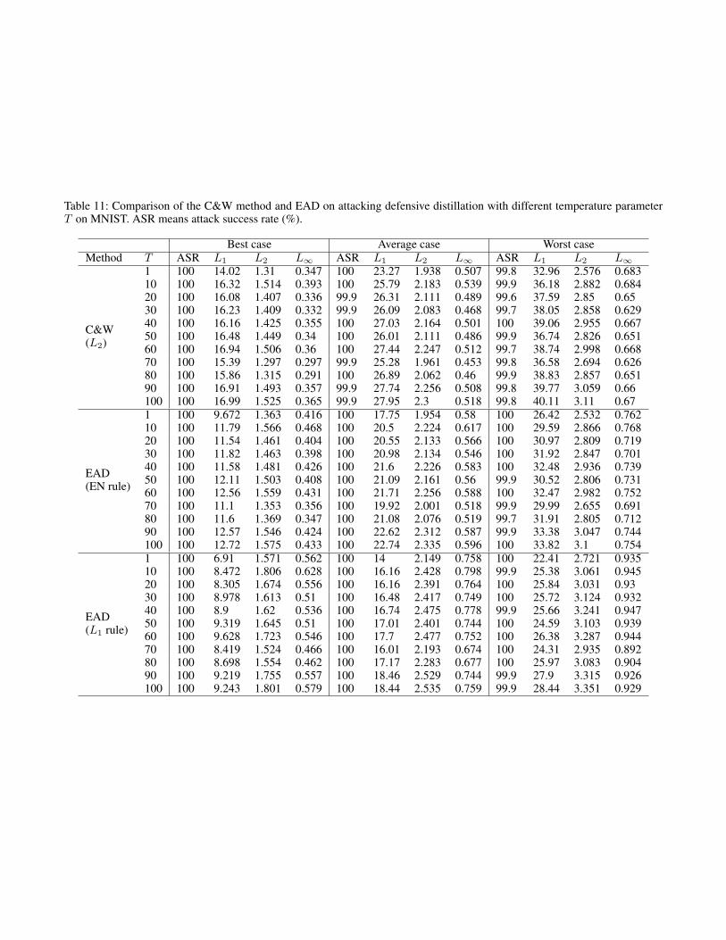
Table 11: Comparison of the C&W method and EAD on attacking defensive distillation with different temperature parameterT on MNIST. ASR means attack success rate (%).

Best case Average case Worst caseMethod T ASR L1 L2 L∞ ASR L1 L2 L∞ ASR L1 L2 L∞

C&W(L2)

1 100 14.02 1.31 0.347 100 23.27 1.938 0.507 99.8 32.96 2.576 0.68310 100 16.32 1.514 0.393 100 25.79 2.183 0.539 99.9 36.18 2.882 0.68420 100 16.08 1.407 0.336 99.9 26.31 2.111 0.489 99.6 37.59 2.85 0.6530 100 16.23 1.409 0.332 99.9 26.09 2.083 0.468 99.7 38.05 2.858 0.62940 100 16.16 1.425 0.355 100 27.03 2.164 0.501 100 39.06 2.955 0.66750 100 16.48 1.449 0.34 100 26.01 2.111 0.486 99.9 36.74 2.826 0.65160 100 16.94 1.506 0.36 100 27.44 2.247 0.512 99.7 38.74 2.998 0.66870 100 15.39 1.297 0.297 99.9 25.28 1.961 0.453 99.8 36.58 2.694 0.62680 100 15.86 1.315 0.291 100 26.89 2.062 0.46 99.9 38.83 2.857 0.65190 100 16.91 1.493 0.357 99.9 27.74 2.256 0.508 99.8 39.77 3.059 0.66100 100 16.99 1.525 0.365 99.9 27.95 2.3 0.518 99.8 40.11 3.11 0.67

EAD(EN rule)

1 100 9.672 1.363 0.416 100 17.75 1.954 0.58 100 26.42 2.532 0.76210 100 11.79 1.566 0.468 100 20.5 2.224 0.617 100 29.59 2.866 0.76820 100 11.54 1.461 0.404 100 20.55 2.133 0.566 100 30.97 2.809 0.71930 100 11.82 1.463 0.398 100 20.98 2.134 0.546 100 31.92 2.847 0.70140 100 11.58 1.481 0.426 100 21.6 2.226 0.583 100 32.48 2.936 0.73950 100 12.11 1.503 0.408 100 21.09 2.161 0.56 99.9 30.52 2.806 0.73160 100 12.56 1.559 0.431 100 21.71 2.256 0.588 100 32.47 2.982 0.75270 100 11.1 1.353 0.356 100 19.92 2.001 0.518 99.9 29.99 2.655 0.69180 100 11.6 1.369 0.347 100 21.08 2.076 0.519 99.7 31.91 2.805 0.71290 100 12.57 1.546 0.424 100 22.62 2.312 0.587 99.9 33.38 3.047 0.744100 100 12.72 1.575 0.433 100 22.74 2.335 0.596 100 33.82 3.1 0.754

EAD(L1 rule)

1 100 6.91 1.571 0.562 100 14 2.149 0.758 100 22.41 2.721 0.93510 100 8.472 1.806 0.628 100 16.16 2.428 0.798 99.9 25.38 3.061 0.94520 100 8.305 1.674 0.556 100 16.16 2.391 0.764 100 25.84 3.031 0.9330 100 8.978 1.613 0.51 100 16.48 2.417 0.749 100 25.72 3.124 0.93240 100 8.9 1.62 0.536 100 16.74 2.475 0.778 99.9 25.66 3.241 0.94750 100 9.319 1.645 0.51 100 17.01 2.401 0.744 100 24.59 3.103 0.93960 100 9.628 1.723 0.546 100 17.7 2.477 0.752 100 26.38 3.287 0.94470 100 8.419 1.524 0.466 100 16.01 2.193 0.674 100 24.31 2.935 0.89280 100 8.698 1.554 0.462 100 17.17 2.283 0.677 100 25.97 3.083 0.90490 100 9.219 1.755 0.557 100 18.46 2.529 0.744 99.9 27.9 3.315 0.926100 100 9.243 1.801 0.579 100 18.44 2.535 0.759 99.9 28.44 3.351 0.929

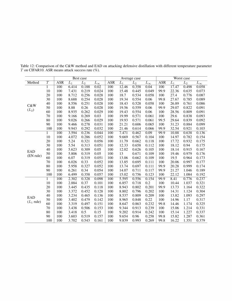
Table 12: Comparison of the C&W method and EAD on attacking defensive distillation with different temperature parameterT on CIFAR10. ASR means attack success rate (%).

Best case Average case Worst caseMethod T ASR L1 L2 L∞ ASR L1 L2 L∞ ASR L1 L2 L∞

C&W(L2)

1 100 6.414 0.188 0.02 100 12.46 0.358 0.04 100 17.47 0.498 0.05810 100 7.431 0.219 0.024 100 15.48 0.445 0.049 99.9 22.36 0.635 0.07320 100 8.712 0.256 0.028 100 18.7 0.534 0.058 100 27.4 0.776 0.08730 100 8.688 0.254 0.028 100 19.34 0.554 0.06 99.8 27.67 0.785 0.08940 100 8.556 0.251 0.028 100 18.43 0.528 0.058 100 26.89 0.761 0.08650 100 8.88 0.26 0.028 100 19.56 0.559 0.06 99.9 29.07 0.822 0.09160 100 8.935 0.262 0.029 100 19.43 0.554 0.06 100 28.56 0.809 0.09170 100 9.166 0.269 0.03 100 19.99 0.571 0.061 100 29.6 0.838 0.09380 100 9.026 0.266 0.029 100 19.93 0.571 0.061 99.5 29.64 0.839 0.09290 100 9.466 0.278 0.031 100 21.21 0.606 0.065 100 31.23 0.884 0.099100 100 9.943 0.292 0.032 100 21.46 0.614 0.066 99.9 32.54 0.921 0.103

EAD(EN rule)

1 100 3.594 0.236 0.044 100 7.471 0.462 0.09 99.9 10.88 0.638 0.13610 100 4.072 0.286 0.052 100 9.669 0.567 0.104 100 14.97 0.782 0.15420 100 5.24 0.321 0.056 100 11.79 0.662 0.118 100 17.72 0.932 0.17530 100 5.54 0.313 0.051 100 12.33 0.658 0.112 100 18.12 0.94 0.17540 100 5.623 0.309 0.05 100 12.02 0.626 0.105 100 18.14 0.915 0.16750 100 5.806 0.319 0.05 100 13 0.671 0.109 100 19.46 0.979 0.17660 100 6.07 0.319 0.051 100 13.06 0.662 0.109 100 19.5 0.964 0.17370 100 6.026 0.33 0.052 100 13.85 0.695 0.111 100 20.06 0.997 0.17780 100 5.958 0.327 0.052 100 13.74 0.697 0.111 99.9 20.28 0.999 0.17490 100 6.261 0.34 0.054 100 14.07 0.711 0.117 99.9 21.27 1.046 0.189100 100 6.499 0.358 0.057 100 15.02 0.756 0.123 100 22.12 1.084 0.192

EAD(L1 rule)

1 100 2.302 0.328 0.098 100 5.595 0.556 0.154 99.9 8.41 0.776 0.23710 100 2.884 0.37 0.101 100 6.857 0.718 0.2 100 10.44 1.037 0.32120 100 3.445 0.435 0.118 100 8.943 0.802 0.201 99.9 13.73 1.164 0.32230 100 3.372 0.452 0.128 100 8.802 0.796 0.202 100 14.31 1.124 0.30440 100 3.234 0.465 0.136 100 8.537 0.809 0.209 100 13.82 1.093 0.29750 100 3.402 0.479 0.142 100 8.965 0.848 0.22 100 14.96 1.17 0.31760 100 3.319 0.497 0.151 100 8.647 0.863 0.232 99.8 14.46 1.174 0.32570 100 3.438 0.506 0.153 100 9.344 0.913 0.239 100 15.06 1.214 0.33180 100 3.418 0.5 0.15 100 9.202 0.914 0.242 100 15.14 1.227 0.33790 100 3.603 0.519 0.157 100 9.654 0.96 0.258 99.8 15.82 1.287 0.361100 100 3.702 0.543 0.161 100 9.839 0.993 0.269 99.8 16.22 1.351 0.379

Table 13: Comparison of attack transferability from the undefended network to the defensively distilled network (T = 100) onMNIST with varying transferability parameter κ. ASR means attack success rate (%). N.A. means not “not available” due tozero ASR. There is no κ parameter for I-FGM.

Best case Average case Worst caseMethod κ ASR L1 L2 L∞ ASR L1 L2 L∞ ASR L1 L2 L∞I-FGM-L1 None 12.2 18.39 1.604 0.418 1.6 19 1.658 0.43 0 N.A. N.A. N.A.I-FGM-L2 None 9.8 17.77 1.537 0.395 1.3 17.25 1.533 0.408 0 N.A. N.A. N.A.I-FGM-L∞ None 14.7 46.38 2.311 0.145 1.7 48.3 2.44 0.158 0 N.A. N.A. N.A.

C&W(L2)

0 5.4 11.13 1.103 0.338 1.1 10.16 1.033 0.343 0 N.A. N.A. N.A.5 16.6 15.58 1.491 0.424 3.4 17.35 1.615 0.46 0 N.A. N.A. N.A.10 42.2 21.94 2.033 0.525 6.5 21.97 2.001 0.527 0 N.A. N.A. N.A.15 74.2 27.65 2.491 0.603 22.6 32.54 2.869 0.671 0.4 56.93 4.628 0.84320 92.9 29.71 2.665 0.639 44.4 38.34 3.322 0.745 2.4 54.25 4.708 0.9125 98.7 30.12 2.719 0.664 62.9 45.41 3.837 0.805 10.9 71.22 5.946 0.97230 99.8 31.17 2.829 0.69 78.1 49.63 4.15 0.847 23 85.93 6.923 0.98735 100 33.27 3.012 0.727 84.2 55.56 4.583 0.886 30.5 105.9 8.072 0.99340 100 36.13 3.255 0.772 87.4 61.25 4.98 0.918 21 125.2 9.09 0.99545 100 39.86 3.553 0.818 85.2 67.82 5.43 0.936 7.4 146.9 10.21 0.99650 100 44.2 3.892 0.868 80.6 70.87 5.639 0.953 0.5 158.4 10.8 0.99655 100 49.37 4.284 0.907 73 76.77 6.034 0.969 0 N.A. N.A. N.A.60 100 54.97 4.703 0.937 67.9 82.07 6.395 0.976 0 N.A. N.A. N.A.

EAD(EN rule)

0 6 8.373 1.197 0.426 0.6 4.876 0.813 0.307 0 N.A. N.A. N.A.5 18.2 11.45 1.547 0.515 2.5 13.07 1.691 0.549 0 N.A. N.A. N.A.10 39.5 15.36 1.916 0.59 8.4 16.45 1.989 0.6 0 N.A. N.A. N.A.15 69.2 19.18 2.263 0.651 19.2 22.74 2.531 0.697 0.4 31.18 3.238 0.84620 89.5 21.98 2.519 0.692 37 28.36 2.99 0.778 1.8 39.91 3.951 0.89725 98.3 23.92 2.694 0.724 58 34.14 3.445 0.831 7.9 49.12 4.65 0.97330 99.9 25.52 2.838 0.748 76.3 40.2 3.909 0.884 23.7 59.9 5.404 0.99335 100 27.42 3.009 0.778 87.9 45.62 4.324 0.92 47.4 70.93 6.176 0.99940 100 30.23 3.248 0.814 95.2 52.33 4.805 0.945 71.3 83.19 6.981 145 100 33.61 3.526 0.857 98 57.75 5.194 0.965 86.2 98.51 7.904 150 100 37.59 3.843 0.899 98.6 66.22 5.758 0.978 87 115.7 8.851 155 100 42.01 4.193 0.934 94.4 70.66 6.09 0.986 44.2 127 9.487 160 100 46.7 4.562 0.961 90 75.59 6.419 0.992 13.3 140.35 10.3 1

EAD(L1 rule)

0 6 6.392 1.431 0.628 0.5 6.57 1.565 0.678 0 N.A. N.A. N.A.5 19 8.914 1.807 0.728 3.2 9.717 1.884 0.738 0 N.A. N.A. N.A.10 40.6 12.16 2.154 0.773 7.5 13.74 2.27 0.8 0 N.A. N.A. N.A.15 70.5 15.39 2.481 0.809 19 18.12 2.689 0.865 0.3 23.15 3.024 0.88420 90 17.73 2.718 0.83 39.4 24.15 3.182 0.902 1.9 38.22 4.173 0.97925 98.6 19.71 2.897 0.851 59.3 30.33 3.652 0.933 7.9 45.74 4.818 0.99730 99.8 21.1 3.023 0.862 76.9 37.38 4.191 0.954 22.2 55.54 5.529 135 100 23 3.186 0.882 89.3 41.13 4.468 0.968 46.8 66.76 6.256 140 100 25.86 3.406 0.904 96.3 47.54 4.913 0.979 69.9 80.05 7.064 145 100 29.4 3.665 0.931 97.6 55.16 5.399 0.988 85.8 96.05 7.94 150 100 33.71 3.957 0.95 98.1 62.01 5.856 0.992 85.7 113.6 8.845 155 100 38.09 4.293 0.971 93.6 65.79 6.112 0.995 43.8 126.4 9.519 160 100 42.7 4.66 0.985 89.6 72.49 6.572 0.997 13 141.3 10.36 1

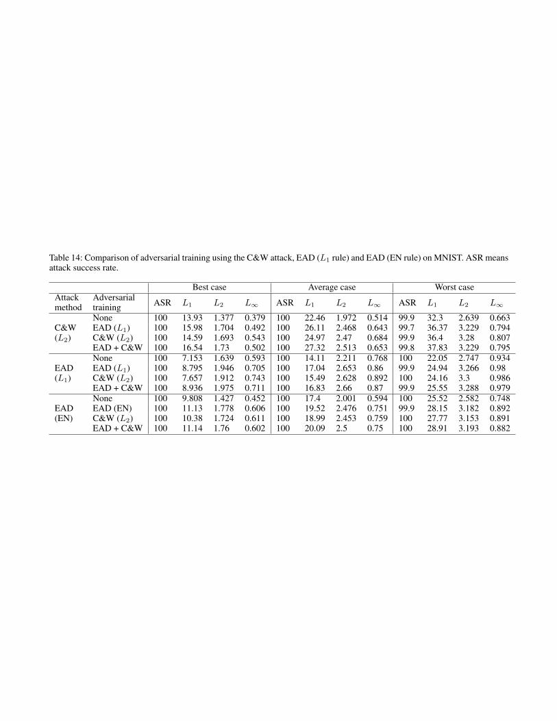
Table 14: Comparison of adversarial training using the C&W attack, EAD (L1 rule) and EAD (EN rule) on MNIST. ASR meansattack success rate.

Best case Average case Worst caseAttackmethod

Adversarialtraining ASR L1 L2 L∞ ASR L1 L2 L∞ ASR L1 L2 L∞

C&W(L2)

None 100 13.93 1.377 0.379 100 22.46 1.972 0.514 99.9 32.3 2.639 0.663EAD (L1) 100 15.98 1.704 0.492 100 26.11 2.468 0.643 99.7 36.37 3.229 0.794C&W (L2) 100 14.59 1.693 0.543 100 24.97 2.47 0.684 99.9 36.4 3.28 0.807EAD + C&W 100 16.54 1.73 0.502 100 27.32 2.513 0.653 99.8 37.83 3.229 0.795

EAD(L1)

None 100 7.153 1.639 0.593 100 14.11 2.211 0.768 100 22.05 2.747 0.934EAD (L1) 100 8.795 1.946 0.705 100 17.04 2.653 0.86 99.9 24.94 3.266 0.98C&W (L2) 100 7.657 1.912 0.743 100 15.49 2.628 0.892 100 24.16 3.3 0.986EAD + C&W 100 8.936 1.975 0.711 100 16.83 2.66 0.87 99.9 25.55 3.288 0.979

EAD(EN)

None 100 9.808 1.427 0.452 100 17.4 2.001 0.594 100 25.52 2.582 0.748EAD (EN) 100 11.13 1.778 0.606 100 19.52 2.476 0.751 99.9 28.15 3.182 0.892C&W (L2) 100 10.38 1.724 0.611 100 18.99 2.453 0.759 100 27.77 3.153 0.891EAD + C&W 100 11.14 1.76 0.602 100 20.09 2.5 0.75 100 28.91 3.193 0.882