Effective Hybrid Stochastic Local SearchAlgorithms for Biobjective Permutation

Flowshop Scheduling

Jeremie Dubois–Lacoste, Manuel Lopez-Ibanez, and Thomas Stutzle

IRIDIA, CoDE, Universite Libre de Bruxelles, Brussels, Belgiumjeremie.dl@gmail.com, {manuel.lopez-ibanez,stuetzle}@ulb.ac.be

Abstract. This paper presents the steps followed in the design of hybridstochastic local search algorithms for biobjective permutation flow shopscheduling problems. In particular, this paper tackles the three pairwisecombinations of the objectives (i) makespan, (ii) the sum of the comple-tion times of the jobs, and (iii) the weighted total tardiness of all jobs.The proposed algorithms are combinations of two local search methods:two-phase local search and Pareto local search. The design of the algo-rithms is based on a careful experimental analysis of crucial algorithmiccomponents of the two search methods. The final results show that thenewly developed algorithms reach very high performance: The solutionsobtained frequently improve upon the best nondominated solutions pre-viously known, while requiring much shorter computation times.

1 Introduction

In this paper, we tackle biobjective flowshop scheduling problems. The flowshopenvironment models problems where each job consists of a set of operations thatare to be carried on machines, and the machine order is the same for each job.Flowshops are a common production environment, for example in the chemicalor the ceramic tile industry. We consider flowshops minimizing the followingcriteria: the completion time of the last job (makespan), which has been themost intensively studied criterion for this problem [1]; the sum of completiontimes (total flowtime) of all jobs, which recently has attracted a lot of efforts[2, 3]; and the weighted tardiness, a criterion which is important in practicalapplications [4]. For an overview of the biobjective flowshop problems that resultfrom each combination of these objectives, we refer to Minella et al. [5].

At a high level, our approach is based on the hypothesis that effective stochas-tic local search (SLS) algorithms for multi-objective combinatorial optimizationproblems (MCOPs) can be obtained by (i) developing (or simply using known)very effective algorithms for the underlying single-objective problems, and (ii)using these single-objective algorithms as components of higher-level algorithmframeworks for tackling multi-objective problems. Further, multi-objective spe-cific local search routines may be examined as an alternative for reaching high-performance algorithms or as a post-processing step.

As a first step in our SLS algorithm development, we adopted the state-of-the-art SLS algorithm for the flowshop problem under makespan objective, theiterated greedy (IG) algorithm of Ruiz and Stutzle [6]. Subsequently, this algo-rithm was extended to the sum of flowtime and weighted tardiness objectivesand we fine-tuned the resulting algorithms. In a next step, we extended thesealgorithms to tackle the biobjective versions of the flowshop problem that resultfrom each of the pairwise combinations of the three above mentioned objectives.This was done by integrating the IG algorithms into the two-phase local search(TPLS) framework [7]. At the same time, we also implemented Pareto localsearch (PLS) [8] algorithms that use different neighborhood structures. A corepart of our work is the careful experimental study of the main algorithmic com-ponents of the resulting TPLS and PLS algorithms. The insights from this studywere then used to propose a hybrid SLS algorithm that combines the TPLS andthe PLS algorithms. The final experimental results with this algorithm show itsexcellent performance: It often finds better Pareto fronts than those of a refer-ence set that was extracted from the best nondominated solutions obtained bya set of 23 other algorithms.

The paper is structured as follows. In Section 2 we introduce basic notionsneeded in the following. In Section 3 we describe the single-objective algorithmsthat underlie the two-phase local search approach. Section 4 presents results ofthe various experimental studies and we conclude in Section 5.

2 Preliminaries

2.1 Multi-objective optimization

In MCOPs, (candidate) solutions are ranked according to an objective functionvector f = (f1, . . . , fd) with d objectives. If no a priori assumptions upon thedecision maker’s preferences can be made, the goal typically becomes to de-termine a set of feasible solutions that “minimize” f in the sense of Paretooptimality. If u and v are vectors in Rd, we say that u dominates v (u ≺ v) iffu 6= v and ui ≤ vi, i = 1, . . . , d; we say that u weakly dominates v (u ≤ v) iffui ≤ vi, i = 1, . . . , d. We also say that u and v are nondominated iff u ⊀ v andv ⊀ u and are (pairwise) non weakly dominated if u 6≤ v and v 6≤ u. For sim-plicity, we also say that a solution s dominates another one s′ iff f(s) ≺ f(s′).If no other s′ exists such that f(s′) ≺ f(s), the solution s is called a Paretooptimum. The goal in MCOPs typically is to determine the set of all Pareto op-timal solutions. Since this task is in many cases computationally intractable, inpractice the goal becomes to find an approximation to the set of Pareto optimalsolutions in a given amount of time that is as good as possible. In fact, any set ofmutually nondominated solutions provides such an approximation. The notionof Pareto optimality can be extended to compare sets of mutually nondominatedsolutions [9]. In particular, we can say that one set A dominates another set B(A ≺ B), iff every b ∈ B is dominated by at least one a ∈ A.

2.2 Bi-objective permutation flowshop scheduling

In the flowshop scheduling problem (FSP) a set of n jobs (J1, . . . , Jn) is given tobe processed on m machines (M1, . . . ,Mm). All jobs go through the machinesin the same order, i.e., all jobs have to be processed first on machine M1, thenon machine M2 and so on until machine Mm. A common restriction in the FSPis to forbid job passing, i.e., the processing sequence of the jobs is the same onall machines. In this case, candidate solutions correspond to permutations ofthe jobs and the resulting problem, on which we focus here, is the permutationflowshop scheduling problem (PFSP). All processing times pij for a job Ji ona machine Mj are fixed, known in advance and nonnegative. In the following,we denote by Ci the completion time of a job Ji on machine Mm. For a givenjob permutation π, the makespan is the completion time of the last job in thepermutation, i.e., Cmax = Cπ(n). For m ≥ 3 this problem is NP-hard in thestrong sense [10]. In the following, we refer to this problem as PFSP -Cmax.

The other objectives we study are the minimization of the sum of flowtimesand the minimization of the weighted tardiness. The sum of flowtimes is definedas

∑ni=1 Ci. The resulting PFSP with this objective is strongly NP-hard even

with only two machines [10]. We refer to this problem as PFSP-SFT. For theweighted tardiness objective, each job has a due date di by which it is to befinished and a weight wi indicating its priority. The tardiness is defined as Ti =max{Ci − di, 0} and the total weighted tardiness is given by

∑ni=1 wi · Ti. This

problem we denote PFSP-WT ; it is strongly NP-hard even for a single machine.In this paper, we tackle the three biobjective problems that result from the

three possible pairs of objectives. A number of algorithms have been proposedto tackle each of these biobjective problems, but rarely more than one possiblecombination of the objectives has been addressed in a paper. The algorithmicapproaches range from constructive algorithms to applications of SLS methodssuch as evolutionary algorithms, tabu search, or simulated annealing. Minella etal. [5] give a comprehensive overview of the literature on the three problems wetackle here and present the results of an extensive experimental analysis of 23algorithms, either specific or adapted for tackling the three biobjective PFSPs.They identify MOSA [11] as the best performing algorithm.

2.3 Two-phase local search and Pareto local search

In this paper, we study SLS algorithms that represent two main classes of multi-objective SLS algorithms [12]: algorithms that follow a component-wise accep-tance criterion (CWAC), and those that follow a scalarized acceptance criterion(SAC). As two paradigmatic examples of each of these classes, we use two-phaselocal search (TPLS) [7] and Pareto local search (PLS) [8].

Two-Phase Local Search. The first phase of TPLS uses an effective single-objective algorithm to find a good solution for one objective. This solution isthe initial solution for the second phase, where a sequence of scalarizations aresolved by an SLS algorithm. Each scalarization transforms the multi-objectiveproblem into a single-objective one using a weighted sum aggregation. For a

Algorithm 1 Two-Phase Local SearchInput: A random or heuristic solution ππ′ := SLS1(π);for all weight vectors λ doπ′ := SLS2(π′,λ);Add π′ to Archive;

end forFilter Archive;

given weight vector λ = (λ1, λ2), the value w of a solution s with objectivefunction vector f(s) = (y1, y2) is computed as w = (λ1 · y1) + (λ2 · y2), s.t.λ1, λ2 ∈ [0, 1] ⊂ R and λ1 + λ2 = 1. In TPLS, each run of the SLS algorithmfor solving a scalarization uses as an initial solution the best one found for theprevious scalarization. The motivation for using such a method is to exploit theeffectiveness of the underlying single-objective algorithm. Algorithm 1 gives thepseudo-code of TPLS. We denote by SLS1 the SLS algorithm to minimize thefirst single objective. SLS2 is the SLS algorithm to minimize the weighted sums.

Pareto Local Search. PLS is an iterative improvement method for solvingMCOPs that is obtained by replacing the usual acceptance criterion of iterativeimprovement algorithms for single-objective problems by an acceptance criterionthat uses the dominance relation. Given an initial archive of unvisited nondom-inated solutions, PLS iteratively applies the following steps. First, it randomlychooses an unvisited solution s from the candidate set. Then, the neighborhoodof s is fully explored and all neighbors that are not weakly dominated by s orby any solution in the archive are added to the archive. Solutions in the archivedominated by the newly added solutions are eliminated. Once the neighborhoodof s is fully explored, s is marked as visited. The algorithm stops when all solu-tions in the archive have been visited.

We also implemented the component-wise step (CW-step) procedure as apost-processing step of the solutions produced by TPLS. It adds nondominatedsolutions in the neighborhood of the solutions returned by TPLS to the archive,but it does not explore the neighborhood of these newly added solutions further.Hence, CW-step may be interpreted as a specific variant of PLS with an earlystopping criterion. Because of this early stopping criterion, the CW-step resultsin worse nondominated sets than PLS. However, compared to running a fullPLS, CW-step typically requires a very small additional computation time.

3 Single-objective SLS algorithms

The performance of the single-objective algorithms used by TPLS is crucial.They should be state-of-the-art algorithms for the underlying single-objectiveproblems and as good as possible for the scalarized problems resulting from theweighted sum aggregations. Motivated by these considerations, for PFSP -Cmax

we reimplemented in C++ the iterated greedy (IG) algorithm (IG-Cmax) by Ruiz

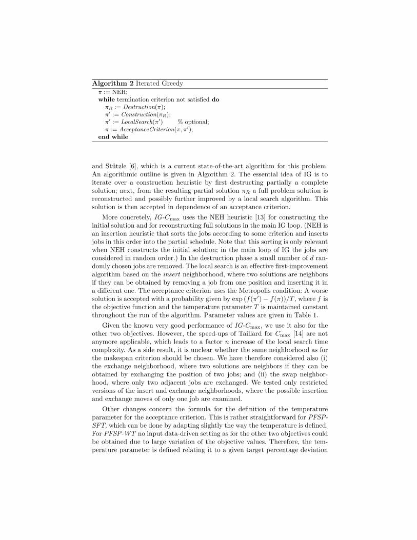
Algorithm 2 Iterated Greedyπ := NEH;while termination criterion not satisfied doπR := Destruction(π);π′ := Construction(πR);π′ := LocalSearch(π′) % optional;π := AcceptanceCriterion(π, π′);

end while

and Stutzle [6], which is a current state-of-the-art algorithm for this problem.An algorithmic outline is given in Algorithm 2. The essential idea of IG is toiterate over a construction heuristic by first destructing partially a completesolution; next, from the resulting partial solution πR a full problem solution isreconstructed and possibly further improved by a local search algorithm. Thissolution is then accepted in dependence of an acceptance criterion.

More concretely, IG-Cmax uses the NEH heuristic [13] for constructing theinitial solution and for reconstructing full solutions in the main IG loop. (NEH isan insertion heuristic that sorts the jobs according to some criterion and insertsjobs in this order into the partial schedule. Note that this sorting is only relevantwhen NEH constructs the initial solution; in the main loop of IG the jobs areconsidered in random order.) In the destruction phase a small number of d ran-domly chosen jobs are removed. The local search is an effective first-improvementalgorithm based on the insert neighborhood, where two solutions are neighborsif they can be obtained by removing a job from one position and inserting it ina different one. The acceptance criterion uses the Metropolis condition: A worsesolution is accepted with a probability given by exp (f(π′)− f(π))/T , where f isthe objective function and the temperature parameter T is maintained constantthroughout the run of the algorithm. Parameter values are given in Table 1.

Given the known very good performance of IG-Cmax, we use it also for theother two objectives. However, the speed-ups of Taillard for Cmax [14] are notanymore applicable, which leads to a factor n increase of the local search timecomplexity. As a side result, it is unclear whether the same neighborhood as forthe makespan criterion should be chosen. We have therefore considered also (i)the exchange neighborhood, where two solutions are neighbors if they can beobtained by exchanging the position of two jobs; and (ii) the swap neighbor-hood, where only two adjacent jobs are exchanged. We tested only restrictedversions of the insert and exchange neighborhoods, where the possible insertionand exchange moves of only one job are examined.

Other changes concern the formula for the definition of the temperatureparameter for the acceptance criterion. This is rather straightforward for PFSP-SFT, which can be done by adapting slightly the way the temperature is defined.For PFSP-WT no input data-driven setting as for the other two objectives couldbe obtained due to large variation of the objective values. Therefore, the tem-perature parameter is defined relating it to a given target percentage deviation

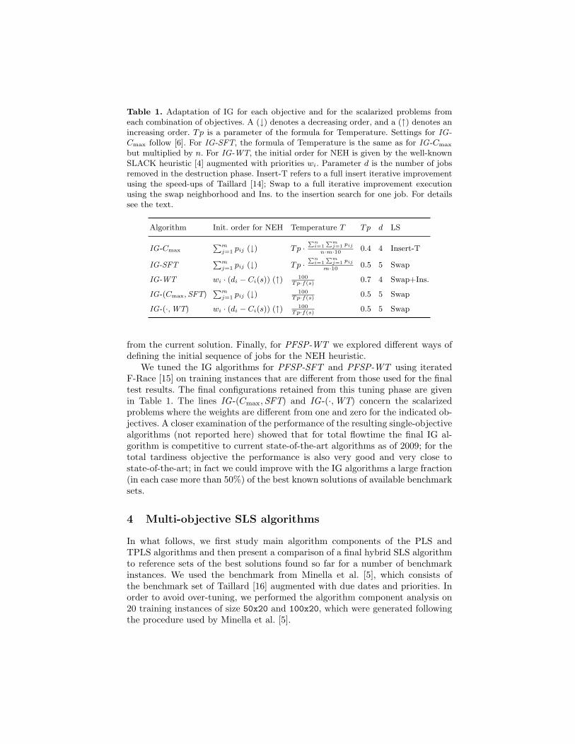
Table 1. Adaptation of IG for each objective and for the scalarized problems fromeach combination of objectives. A (↓) denotes a decreasing order, and a (↑) denotes anincreasing order. Tp is a parameter of the formula for Temperature. Settings for IG-Cmax follow [6]. For IG-SFT, the formula of Temperature is the same as for IG-Cmax

but multiplied by n. For IG-WT, the initial order for NEH is given by the well-knownSLACK heuristic [4] augmented with priorities wi. Parameter d is the number of jobsremoved in the destruction phase. Insert-T refers to a full insert iterative improvementusing the speed-ups of Taillard [14]; Swap to a full iterative improvement executionusing the swap neighborhood and Ins. to the insertion search for one job. For detailssee the text.

Algorithm Init. order for NEH Temperature T Tp d LS

IG-Cmax

Pmj=1 pij (↓) Tp ·

Pni=1

Pmj=1 pij

n·m·10 0.4 4 Insert-T

IG-SFTPm

j=1 pij (↓) Tp ·Pn

i=1Pm

j=1 pij

m·10 0.5 5 Swap

IG-WT wi · (di − Ci(s)) (↑) 100Tp·f(s)

0.7 4 Swap+Ins.

IG-(Cmax,SFT)Pm

j=1 pij (↓) 100Tp·f(s)

0.5 5 Swap

IG-(·,WT) wi · (di − Ci(s)) (↑) 100Tp·f(s)

0.5 5 Swap

from the current solution. Finally, for PFSP-WT we explored different ways ofdefining the initial sequence of jobs for the NEH heuristic.

We tuned the IG algorithms for PFSP-SFT and PFSP-WT using iteratedF-Race [15] on training instances that are different from those used for the finaltest results. The final configurations retained from this tuning phase are givenin Table 1. The lines IG-(Cmax,SFT) and IG-(·,WT) concern the scalarizedproblems where the weights are different from one and zero for the indicated ob-jectives. A closer examination of the performance of the resulting single-objectivealgorithms (not reported here) showed that for total flowtime the final IG al-gorithm is competitive to current state-of-the-art algorithms as of 2009; for thetotal tardiness objective the performance is also very good and very close tostate-of-the-art; in fact we could improve with the IG algorithms a large fraction(in each case more than 50%) of the best known solutions of available benchmarksets.

4 Multi-objective SLS algorithms

In what follows, we first study main algorithm components of the PLS andTPLS algorithms and then present a comparison of a final hybrid SLS algorithmto reference sets of the best solutions found so far for a number of benchmarkinstances. We used the benchmark from Minella et al. [5], which consists ofthe benchmark set of Taillard [16] augmented with due dates and priorities. Inorder to avoid over-tuning, we performed the algorithm component analysis on20 training instances of size 50x20 and 100x20, which were generated followingthe procedure used by Minella et al. [5].

6500 6700 6900 71003800

0040

0000

4200

00

Objectives: Cmax and ∑∑Cj

Cmax

∑∑C

j

●

●

●

random setheuristic setIG setheuristic seedsIG seeds

6600 7000 7400 78005e+

057e

+05

9e+

05

Objectives: Cmax and ∑∑wjTj

Cmax

∑∑w

jTj

●

●

●

random setheuristic setIG setheuristic seedsIG seeds

380000 400000 420000

6e+

058e

+05

1e+

06

Objectives: ∑∑Cj and ∑∑wjTj

∑∑Cj

∑∑w

jTj

●

●

●

random setheuristic setIG setheuristic seedsIG seeds

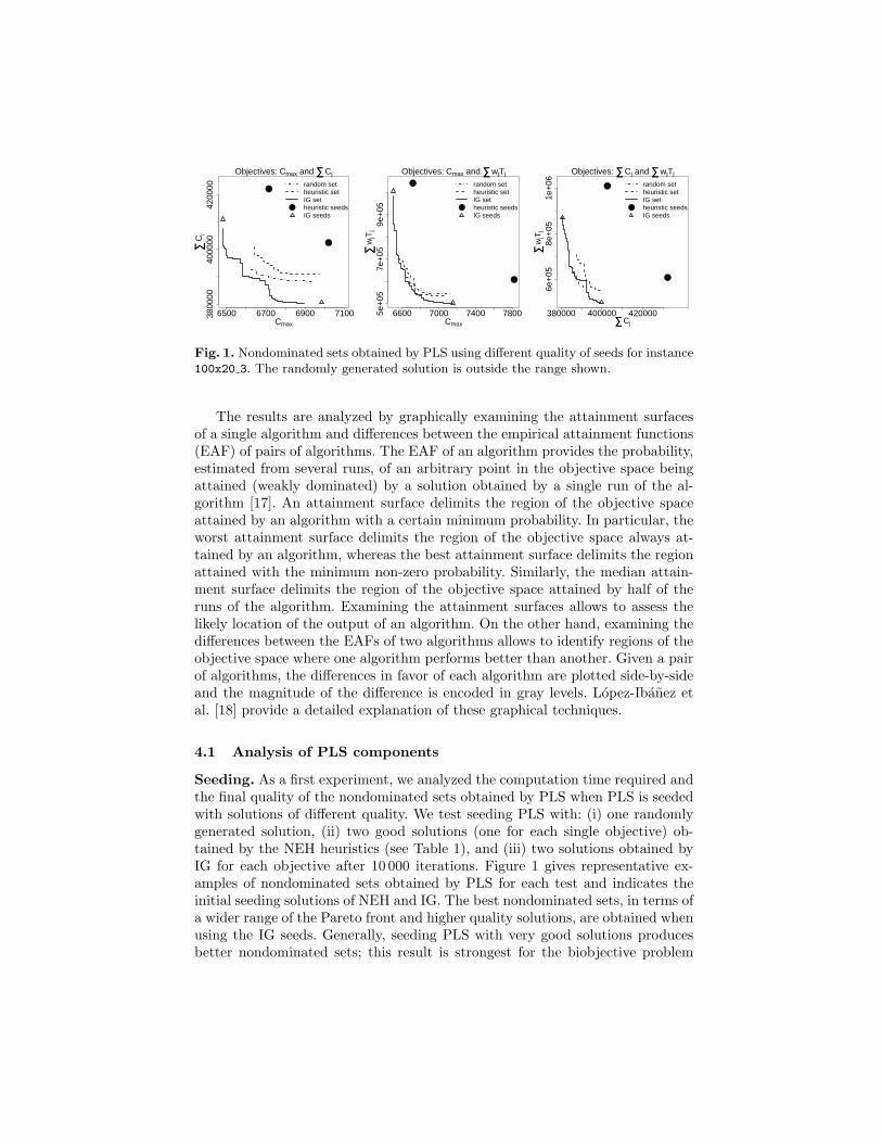
Fig. 1. Nondominated sets obtained by PLS using different quality of seeds for instance100x20 3. The randomly generated solution is outside the range shown.

The results are analyzed by graphically examining the attainment surfacesof a single algorithm and differences between the empirical attainment functions(EAF) of pairs of algorithms. The EAF of an algorithm provides the probability,estimated from several runs, of an arbitrary point in the objective space beingattained (weakly dominated) by a solution obtained by a single run of the al-gorithm [17]. An attainment surface delimits the region of the objective spaceattained by an algorithm with a certain minimum probability. In particular, theworst attainment surface delimits the region of the objective space always at-tained by an algorithm, whereas the best attainment surface delimits the regionattained with the minimum non-zero probability. Similarly, the median attain-ment surface delimits the region of the objective space attained by half of theruns of the algorithm. Examining the attainment surfaces allows to assess thelikely location of the output of an algorithm. On the other hand, examining thedifferences between the EAFs of two algorithms allows to identify regions of theobjective space where one algorithm performs better than another. Given a pairof algorithms, the differences in favor of each algorithm are plotted side-by-sideand the magnitude of the difference is encoded in gray levels. Lopez-Ibanez etal. [18] provide a detailed explanation of these graphical techniques.

4.1 Analysis of PLS components

Seeding. As a first experiment, we analyzed the computation time required andthe final quality of the nondominated sets obtained by PLS when PLS is seededwith solutions of different quality. We test seeding PLS with: (i) one randomlygenerated solution, (ii) two good solutions (one for each single objective) ob-tained by the NEH heuristics (see Table 1), and (iii) two solutions obtained byIG for each objective after 10 000 iterations. Figure 1 gives representative ex-amples of nondominated sets obtained by PLS for each test and indicates theinitial seeding solutions of NEH and IG. The best nondominated sets, in terms ofa wider range of the Pareto front and higher quality solutions, are obtained whenusing the IG seeds. Generally, seeding PLS with very good solutions producesbetter nondominated sets; this result is strongest for the biobjective problem

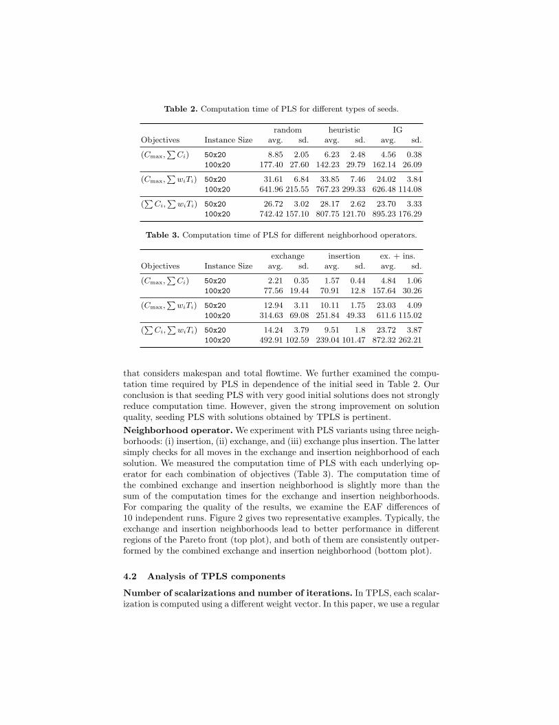
Table 2. Computation time of PLS for different types of seeds.

random heuristic IGObjectives Instance Size avg. sd. avg. sd. avg. sd.

(Cmax,PCi) 50x20 8.85 2.05 6.23 2.48 4.56 0.38

100x20 177.40 27.60 142.23 29.79 162.14 26.09

(Cmax,PwiTi) 50x20 31.61 6.84 33.85 7.46 24.02 3.84

100x20 641.96 215.55 767.23 299.33 626.48 114.08

(PCi,

PwiTi) 50x20 26.72 3.02 28.17 2.62 23.70 3.33

100x20 742.42 157.10 807.75 121.70 895.23 176.29

Table 3. Computation time of PLS for different neighborhood operators.

exchange insertion ex. + ins.Objectives Instance Size avg. sd. avg. sd. avg. sd.

(Cmax,PCi) 50x20 2.21 0.35 1.57 0.44 4.84 1.06

100x20 77.56 19.44 70.91 12.8 157.64 30.26

(Cmax,PwiTi) 50x20 12.94 3.11 10.11 1.75 23.03 4.09

100x20 314.63 69.08 251.84 49.33 611.6 115.02

(PCi,

PwiTi) 50x20 14.24 3.79 9.51 1.8 23.72 3.87

100x20 492.91 102.59 239.04 101.47 872.32 262.21

that considers makespan and total flowtime. We further examined the compu-tation time required by PLS in dependence of the initial seed in Table 2. Ourconclusion is that seeding PLS with very good initial solutions does not stronglyreduce computation time. However, given the strong improvement on solutionquality, seeding PLS with solutions obtained by TPLS is pertinent.Neighborhood operator. We experiment with PLS variants using three neigh-borhoods: (i) insertion, (ii) exchange, and (iii) exchange plus insertion. The lattersimply checks for all moves in the exchange and insertion neighborhood of eachsolution. We measured the computation time of PLS with each underlying op-erator for each combination of objectives (Table 3). The computation time ofthe combined exchange and insertion neighborhood is slightly more than thesum of the computation times for the exchange and insertion neighborhoods.For comparing the quality of the results, we examine the EAF differences of10 independent runs. Figure 2 gives two representative examples. Typically, theexchange and insertion neighborhoods lead to better performance in differentregions of the Pareto front (top plot), and both of them are consistently outper-formed by the combined exchange and insertion neighborhood (bottom plot).

4.2 Analysis of TPLS components

Number of scalarizations and number of iterations. In TPLS, each scalar-ization is computed using a different weight vector. In this paper, we use a regular

3.8e+05 3.86e+05 3.92e+05 3.98e+05∑Ci

5e+

05

6e+

05

7e+

05

8e+

05

∑w

iTi

[0.8, 1.0][0.6, 0.8)[0.4, 0.6)[0.2, 0.4)[0.0, 0.2)

3.8e+05 3.86e+05 3.92e+05 3.98e+05∑Ci

5e+

05

6e+

05

7e+

05

8e+

05

∑w

iTi

3.8e+05 3.86e+05 3.92e+05 3.98e+05∑Ci

5e+

05

6e+

05

7e+

05

8e+

05

∑w

iTi

[0.8, 1.0][0.6, 0.8)[0.4, 0.6)[0.2, 0.4)[0.0, 0.2)

3.8e+05 3.86e+05 3.92e+05 3.98e+05∑Ci

5e+

05

6e+

05

7e+

05

8e+

05

∑w

iTi

Fig. 2. EAF differences for (top) insertion vs. exchange and (bottom) exchange vs.exchange and insertion. The combination of objectives is

PCi and

PwiTi. Dashed

lines are the median attainment surfaces of each algorithm. Black lines correspond tothe overall best and overall worst attainment surfaces of both algorithms.

sequence of weight vectors from λ = (1, 0) to λ = (0, 1). If Nscalar is the num-ber of scalarizations, the successive scalarizations are defined by weight vectorsλi = (1− (i/Nscalar), i/Nscalar), i = 0, . . . , Nscalar.

For a fixed computation time, in TPLS there is a tradeoff between the numberof scalarizations to be used and the number of iterations to be given for eachof the invocations of the single-objective SLS algorithm. In fact, the number ofscalarizations (Nscalar) determines how many scalarized problems will be solved(intuitively, the more the better approximations to the Pareto front may beobtained), while the number of iterations (Niter) of IG determines decisivelyhow good the final IG solution will be. Here, we examine the trade-off betweenthe settings of these two parameters by testing all 9 combinations of the followingsettings: Nscalar = {10, 31, 100} and Niter = {100, 1 000, 10 000}.

6350 6450 6550 6650 6750 6850Cmax

3.7

5e+

05

3.8

5e+

05

3.9

5e+

05

∑C

i

[0.8, 1.0][0.6, 0.8)[0.4, 0.6)[0.2, 0.4)[0.0, 0.2)

6350 6450 6550 6650 6750 6850Cmax

3.7

5e+

05

3.8

5e+

05

3.9

5e+

05

∑C

i

6350 6500 6650 6800 6950Cmax

5e+

05

6e+

05

7e+

05

8e+

05

9e+

05

∑w

iTi

[0.8, 1.0][0.6, 0.8)[0.4, 0.6)[0.2, 0.4)[0.0, 0.2)

6350 6500 6650 6800 6950Cmax

5e+

05

6e+

05

7e+

05

8e+

05

9e+

05

∑w

iTi

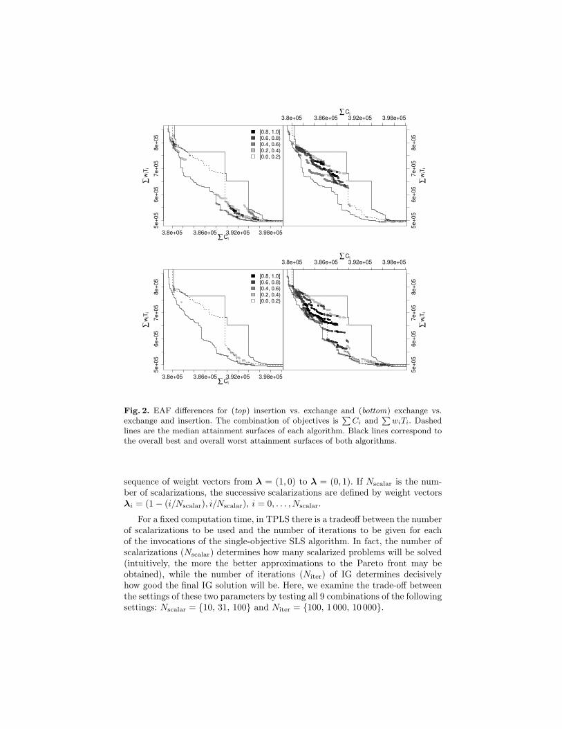
Fig. 3. EAF differences between Nscalar = 100 and Niter = 1000, versus Nscalar = 10and Niter = 10000 for two combinations of objectives: Cmax and

PCi (top) and Cmax

andPwiTi (bottom).

We first studied the impact of increasing either Nscalar or Niter for a fixedsetting of the other parameter. Although clear improvements are obtained byincreasing each of the two parameters, there are significant differences. Whilefor the number of scalarizations some type of limiting behavior without strongimprovements was observed when going from 31 to 100 scalarizations (while im-provements from 10 to 31 were considerable), increasing the number of iterationsof IG alone seems always to produce significant improvements.

Next, we compare settings that require roughly the same computation time.Figure 3 compares a configuration of TPLS using Nscalar = 100 and Niter = 1000against other configuration using Nscalar = 10 and Niter = 10000. Results areshown for two of the three combinations of objective functions. (The resultsare representative for other instances.) As illustrated by the plots, there is noclear winner in this case. A larger number of iterations typically produces bettersolutions in the extremes of the Pareto front. On the other hand, a larger number

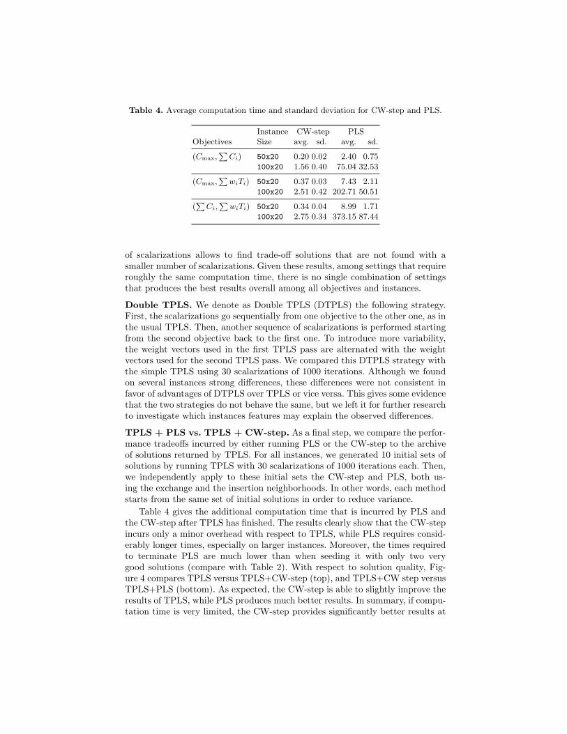
Table 4. Average computation time and standard deviation for CW-step and PLS.

Instance CW-step PLSObjectives Size avg. sd. avg. sd.

(Cmax,PCi) 50x20 0.20 0.02 2.40 0.75

100x20 1.56 0.40 75.04 32.53

(Cmax,PwiTi) 50x20 0.37 0.03 7.43 2.11

100x20 2.51 0.42 202.71 50.51

(PCi,

PwiTi) 50x20 0.34 0.04 8.99 1.71

100x20 2.75 0.34 373.15 87.44

of scalarizations allows to find trade-off solutions that are not found with asmaller number of scalarizations. Given these results, among settings that requireroughly the same computation time, there is no single combination of settingsthat produces the best results overall among all objectives and instances.

Double TPLS. We denote as Double TPLS (DTPLS) the following strategy.First, the scalarizations go sequentially from one objective to the other one, as inthe usual TPLS. Then, another sequence of scalarizations is performed startingfrom the second objective back to the first one. To introduce more variability,the weight vectors used in the first TPLS pass are alternated with the weightvectors used for the second TPLS pass. We compared this DTPLS strategy withthe simple TPLS using 30 scalarizations of 1000 iterations. Although we foundon several instances strong differences, these differences were not consistent infavor of advantages of DTPLS over TPLS or vice versa. This gives some evidencethat the two strategies do not behave the same, but we left it for further researchto investigate which instances features may explain the observed differences.

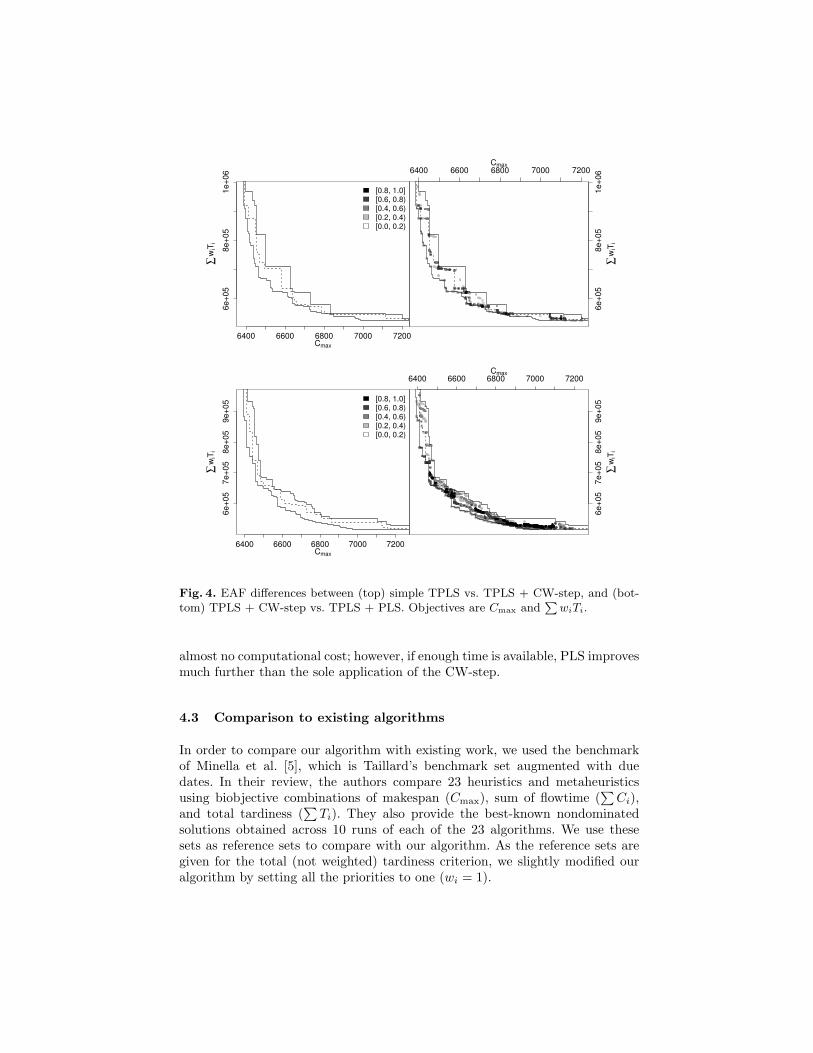
TPLS + PLS vs. TPLS + CW-step. As a final step, we compare the perfor-mance tradeoffs incurred by either running PLS or the CW-step to the archiveof solutions returned by TPLS. For all instances, we generated 10 initial sets ofsolutions by running TPLS with 30 scalarizations of 1000 iterations each. Then,we independently apply to these initial sets the CW-step and PLS, both us-ing the exchange and the insertion neighborhoods. In other words, each methodstarts from the same set of initial solutions in order to reduce variance.

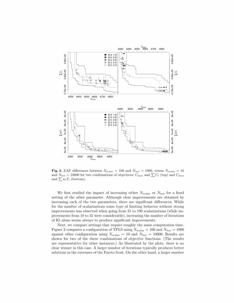
Table 4 gives the additional computation time that is incurred by PLS andthe CW-step after TPLS has finished. The results clearly show that the CW-stepincurs only a minor overhead with respect to TPLS, while PLS requires consid-erably longer times, especially on larger instances. Moreover, the times requiredto terminate PLS are much lower than when seeding it with only two verygood solutions (compare with Table 2). With respect to solution quality, Fig-ure 4 compares TPLS versus TPLS+CW-step (top), and TPLS+CW step versusTPLS+PLS (bottom). As expected, the CW-step is able to slightly improve theresults of TPLS, while PLS produces much better results. In summary, if compu-tation time is very limited, the CW-step provides significantly better results at

6400 6600 6800 7000 7200Cmax

6e+

05

8e+

05

1e+

06

∑w

iTi

[0.8, 1.0][0.6, 0.8)[0.4, 0.6)[0.2, 0.4)[0.0, 0.2)

6400 6600 6800 7000 7200Cmax

6e+

05

8e+

05

1e+

06

∑w

iTi

6400 6600 6800 7000 7200Cmax

6e+

05

7e+

05

8e+

05

9e+

05

∑w

iTi

[0.8, 1.0][0.6, 0.8)[0.4, 0.6)[0.2, 0.4)[0.0, 0.2)

6400 6600 6800 7000 7200Cmax

6e+

05

7e+

05

8e+

05

9e+

05

∑w

iTi

Fig. 4. EAF differences between (top) simple TPLS vs. TPLS + CW-step, and (bot-tom) TPLS + CW-step vs. TPLS + PLS. Objectives are Cmax and

PwiTi.

almost no computational cost; however, if enough time is available, PLS improvesmuch further than the sole application of the CW-step.

4.3 Comparison to existing algorithms

In order to compare our algorithm with existing work, we used the benchmarkof Minella et al. [5], which is Taillard’s benchmark set augmented with duedates. In their review, the authors compare 23 heuristics and metaheuristicsusing biobjective combinations of makespan (Cmax), sum of flowtime (

∑Ci),

and total tardiness (∑Ti). They also provide the best-known nondominated

solutions obtained across 10 runs of each of the 23 algorithms. We use thesesets as reference sets to compare with our algorithm. As the reference sets aregiven for the total (not weighted) tardiness criterion, we slightly modified ouralgorithm by setting all the priorities to one (wi = 1).

In particular, we compare our results with the reference sets given for acomputation time of 200 seconds and corresponding to instances from ta081 tota090 (size 100x20). These reference sets were obtained on an Intel Dual CoreE6600 CPU running at 2.4 Ghz. By comparison, our algorithms were run on aIntel Xeon E5410 CPU running at 2.33 Ghz with 6MB of cache size, under Clus-ter Rocks Linux. Both machines result in approximately similar speed, however,to be conservative, we decided to round down the quality of our results by usingonly 150 CPU seconds. For our algorithms, we used the following parametersettings. The two extreme solutions are generated by running IG for 10 secondseach. Then TPLS starts from the solution obtained for the first objective andruns 14 scalarizations of 5 seconds each. Finally, we apply PLS in the exchangeand insertion neighborhoods and stop it after 60 CPU seconds. We repeat eachrun 10 times with different random seeds.

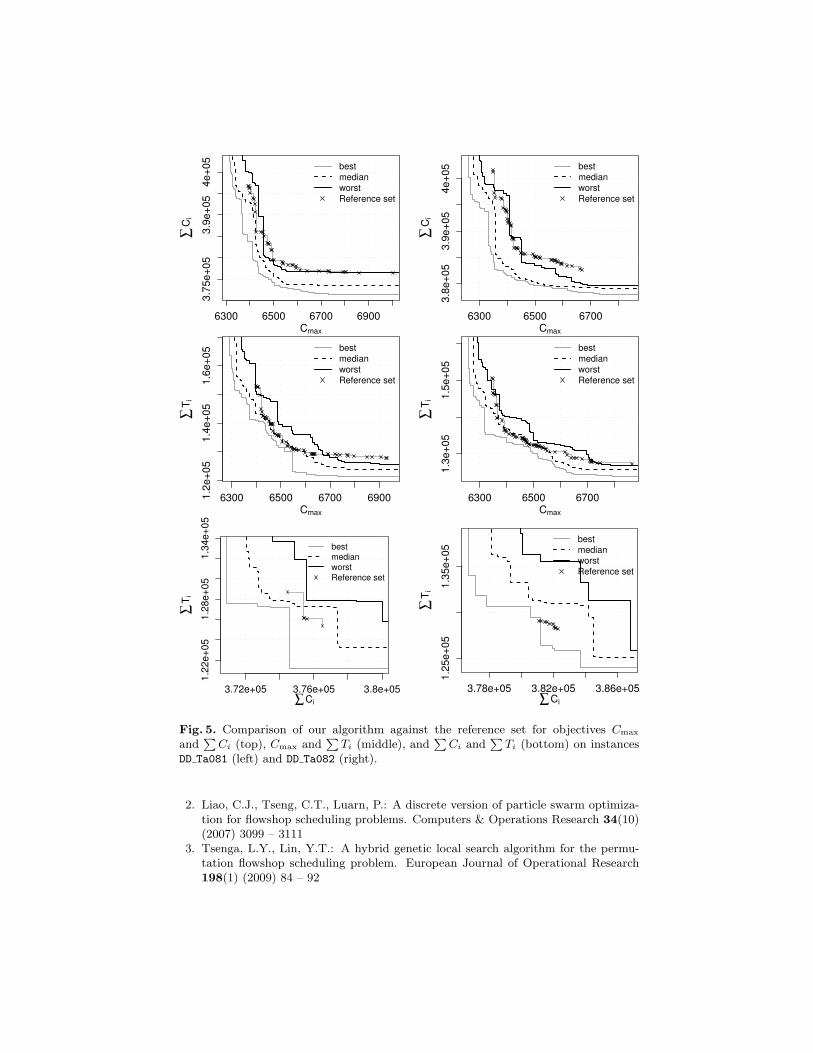
For each instance, we compare the best, median and worst attainment sur-faces obtained by our algorithm with the corresponding reference set. Figure5 shows results for the three objective combinations. In most cases, the me-dian attainment surface of our algorithm is very close to (and often domi-nates) the reference set obtained by 10 runs of 23 algorithms, each run us-ing 200 CPU seconds. Moreover, the current state-of-the-art algorithms forthese problems are among these algorithms. Therefore, we conclude that ouralgorithm is clearly competitive and probably superior to the current state-of-the-art for these problems. All the additional plots are available online athttp://iridia.ulb.ac.be/supp/IridiaSupp2009-004

5 Conclusions

In this paper, we have studied algorithmic components of the TPLS and PLS al-gorithms for three biobjective permutation flowshop problems, and we proposeda hybrid, high-performing SLS algorithm for these problems.

The final experimental results have shown that our SLS algorithms are able tosignificantly improve upon the reference sets of the nondominated solutions thathave been obtained during an extensive experimental study of 23 algorithms forthe same biobjective problems. These and other recent results in the literature[7, 19] suggest that hybrid algorithms combining the TPLS and PLS frameworkshave a large potential to improve upon the current state-of-the-art in multi-objective optimization.

Acknowledgments. This work was supported by the META-X project, anAction de Recherche Concertee funded by the Scientific Research Directorate ofthe French Community of Belgium. Thomas Stutzle acknowledges support fromthe Belgian F.R.S.-FNRS, of which he is a Research Associate.

References

1. Ruiz, R., Maroto, C.: A comprehensive review and evaluation of permutation flow-shop heuristics. European Journal of Operational Research 165 (2005) 479–494

6300 6500 6700 6900

Cmax

3.7

5e

+0

53.9

e+

05

4e

+05

∑C

i

best

median

worst

Reference set

6300 6500 6700

Cmax

3.8

e+

05

3.9

e+

05

4e+

05

∑C

i

best

median

worst

Reference set

6300 6500 6700 6900

Cmax

1.2

e+

05

1.4

e+

05

1.6

e+

05

∑T

i

best

median

worst

Reference set

6300 6500 6700

Cmax

1.3

e+

05

1.5

e+

05

∑T

i

best

median

worst

Reference set

3.72e+05 3.76e+05 3.8e+05

∑Ci

1.2

2e+

05

1.2

8e+

05

1.3

4e+

05

∑T

i

best

median

worst

Reference set

3.78e+05 3.82e+05 3.86e+05

∑Ci

1.2

5e

+0

51

.35

e+

05

∑T

i

best

median

worst

Reference set

Fig. 5. Comparison of our algorithm against the reference set for objectives Cmax

andPCi (top), Cmax and

PTi (middle), and

PCi and

PTi (bottom) on instances

DD Ta081 (left) and DD Ta082 (right).

2. Liao, C.J., Tseng, C.T., Luarn, P.: A discrete version of particle swarm optimiza-tion for flowshop scheduling problems. Computers & Operations Research 34(10)(2007) 3099 – 3111

3. Tsenga, L.Y., Lin, Y.T.: A hybrid genetic local search algorithm for the permu-tation flowshop scheduling problem. European Journal of Operational Research198(1) (2009) 84 – 92

4. Vallada, E., Ruiz, R., Minella, G.: Minimising total tardiness in the m-machineflowshop problem: A review and evaluation of heuristics and metaheuristics. Com-puters & Operations Research 35(4) (2008) 1350–1373

5. Minella, G., Ruiz, R., Ciavotta, M.: A review and evaluation of multiobjectivealgorithms for the flowshop scheduling problem. INFORMS Journal on Computing20(3) (2008) 451–471

6. Ruiz, R., Stutzle, T.: A simple and effective iterated greedy algorithm for the per-mutation flowshop scheduling problem. European Journal of Operational Research177(3) (2007) 2033–2049

7. Paquete, L., Stutzle, T.: A two-phase local search for the biobjective travelingsalesman problem. In Fonseca, C.M., et al., eds.: EMO 2003. Volume 2632 ofLNCS., Heidelberg, Springer Verlag (2003) 479–493

8. Paquete, L., Chiarandini, M., Stutzle, T.: Pareto local optimum sets in the biob-jective traveling salesman problem: An experimental study. In Gandibleux, X.,et al., eds.: Metaheuristics for Multiobjective Optimisation. Volume 535 of LNEMS.Springer Verlag (2004) 177–200

9. Zitzler, E., Thiele, L., Laumanns, M., Fonseca, C.M., Grunert da Fonseca, V.: Per-formance assessment of multiobjective optimizers: An analysis and review. IEEETransactions on Evolutionary Computation 7(2) (2003) 117–132

10. Garey, M.R., Johnson, D.S., Sethi, R.: The complexity of flowshop and jobshopscheduling. Mathematics of Operations Research 1 (1976) 117–129

11. Varadharajan, T.K., Rajendran, C.: A multi-objective simulated-annealing algo-rithm for scheduling in flowshops to minimize the makespan and total flowtime ofjobs. European Journal of Operational Research 167(3) (2005) 772–795

12. Paquete, L., Stutzle, T.: Stochastic local search algorithms for multiobjective com-binatorial optimization: A review. In Gonzalez, T.F., ed.: Handbook of Approxima-tion Algorithms and Metaheuristics. Chapman & Hall/CRC (2007) 29–1—29–15

13. Nawaz, M., Jr., E.E., Ham, I.: A heuristic algorithm for the m-machine, n-jobflow-shop sequencing problem. OMEGA 11(1) (1983) 91–95

14. Taillard, E.D.: Some efficient heuristic methods for the flow shop sequencing prob-lem. European Journal of Operational Research 47(1) (1990) 65–74

15. Balaprakash, P., Birattari, M., Stutzle, T.: Improvement strategies for the F-Racealgorithm: Sampling design and iterative refinement. In Bartz-Beielstein, T., et al.,eds.: HM 2007. Volume 4771 of LNCS., Heidelberg, Springer Verlag (2007) 108–122

16. Taillard, E.D.: Benchmarks for basic scheduling problems. European Journal ofOperational Research 64(2) (1993) 278–285

17. Grunert da Fonseca, V., Fonseca, C.M., Hall, A.: Inferential performance assess-ment of stochastic optimizers and the attainment function. In Zitzler, E., et al.,eds.: EMO 2001. Volume 1993 of LNCS., Heidelberg, Springer Verlag (2001) 213–225

18. Lopez-Ibanez, M., Paquete, L., Stutzle, T.: Exploratory analysis of stochastic localsearch algorithms in biobjective optimization. Technical Report TR/IRIDIA/2009-015, IRIDIA, Universite Libre de Bruxelles, Brussels, Belgium (May 2009)

19. Lust, T., Teghem, J.: Two-phase Pareto local search for the biobjective travelingsalesman problem. Journal of Heuristics (2009) DOI: 10.1007/s10732-009-9103-9To appear.