DZDDPZ8 Fourierova t., spectral enhancement …homel.vsb.cz/~hor10/Vyuka/DZDPZ/DZDDPZEN8.pdfDoc. Dr....
57
DZDDPZ8 – Fourierova t., spectral enhancement Doc. Dr. Ing. Jiří Horák - Ing. Tomáš Peňáz, Ph.D. Institut geoinformatiky VŠB-TU Ostrava
Transcript of DZDDPZ8 Fourierova t., spectral enhancement …homel.vsb.cz/~hor10/Vyuka/DZDPZ/DZDDPZEN8.pdfDoc. Dr....

DZDDPZ8 – Fourierova t., spectral enhancement
Doc. Dr. Ing. Jiří Horák - Ing. Tomáš Peňáz, Ph.D.
Institut geoinformatiky
VŠB-TU Ostrava
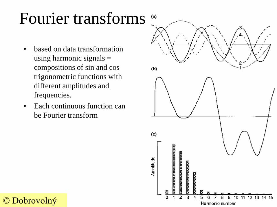
Fourier transforms
• based on data transformation
using harmonic signals =
compositions of sin and cos
trigonometric functions with
different amplitudes and
frequencies.
• Each continuous function can
be Fourier transform
© Dobrovolný

Fourier transforms
• The result can be displayed as Fourier spectrum
• identified low frequencies are recorded near the spectre centre
• high frequencies are recorded near the edges
• orientation of edges or lines in the image is also important –
they are displayed perpendicularly to the original direction
• in the Fourier spectrum, the horizontal lines appear as vertical
lines
• Shades of grey in the Fourier spectrum indicate the count of the
respective frequency.
© Dobrovolný

Procedure of Fourier transforms
• the image is transformed into the Fourier
spectrum using fast Fourier transforms (FFT)
• suitable filters are applied to this spectrum;
• the result is then transformed back into an
image using inverse Fourier transforms (IFT)
• remove noise - apply a circular filter to the
spectrum, keeping only the inner part of the
circle (low frequencies).
• to highlight high frequencies - use a circular
filter retaining the outer part of the spectrum.
• to cancel lines of a certain direction - apply a
wedge filter of perpendicular direction.
© Dobrovolný

© Dobrovolný

© Dobrovolný

© Dobrovolný

Spectral enhancement • manipulation with multi-images
• division of the image and the use of ratios of image
bands
• we can distinguish subtle spectral changes
• highlight changes in the inclination of spectral
reflectance curves regardless of the absolute values
• From n bands IT - create n*(n-1) ratios or 1/2
(regardless of order).
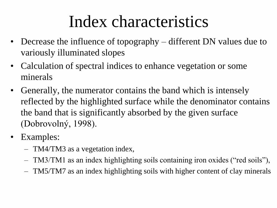
Index characteristics • Decrease the influence of topography – different DN values due to
variously illuminated slopes
• Calculation of spectral indices to enhance vegetation or some
minerals
• Generally, the numerator contains the band which is intensely
reflected by the highlighted surface while the denominator contains
the band that is significantly absorbed by the given surface
(Dobrovolný, 1998).
• Examples:
– TM4/TM3 as a vegetation index,
– TM3/TM1 as an index highlighting soils containing iron oxides (“red soils”),
– TM5/TM7 as an index highlighting soils with higher content of clay minerals

optimum index factor • Synthesis from bands with the most different information
• OIF
• sk standard deviation of the k-band
• rj correlation coefficient between two included bands
• Composition (synthesis) with the highest OIF – provide the greatest
benefit (theoretically)
• Recommendation what bands should be included

• If the final image contains only ratios for
synthesis, the information on absolute values may
be missing. If one original band is also used, we
get a hybrid synthesis.
• As with other forms of image enhancement, pre-
processing is recommended.
• Especially when using ratios, it is necessary to
remove noise such as atmospheric haze
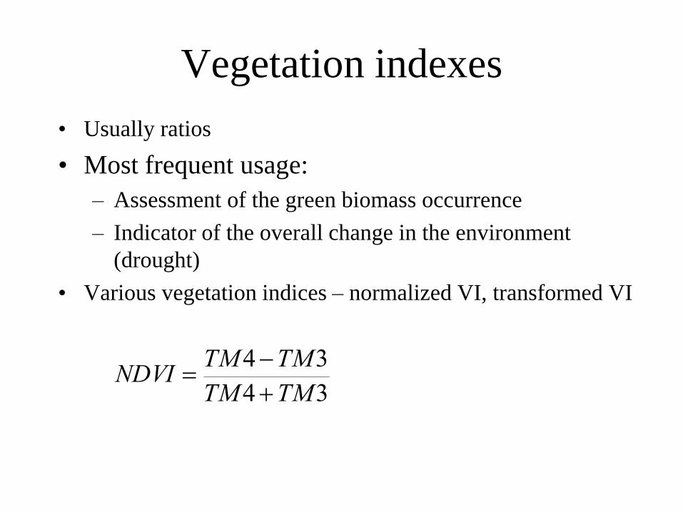
Vegetation indexes
• Usually ratios
• Most frequent usage:
– Assessment of the green biomass occurrence
– Indicator of the overall change in the environment
(drought)
• Various vegetation indices – normalized VI, transformed VI
34
34
TMTM
TMTMNDVI

Principle of the calculation of vegetation indices
• Based on
– High interaction of health vegetation with VIS and NIR
radiation
– specific spectral behaviour of vegetation (see basic course
of RS!)
– Different behaviour of other materials (land cover)

Classification of vegetation indexes
• Vegetation indexes
– empirical
– optimalized
• Vegetation indexes (Jackson, Huete, 1991)
– Slope-based
– ratio
– ortogonal
– transformed

Empirical vegetation indexes
• Detection of vegetation occurrence
• The result has no exact physical meaning
• Not quantitative assessment but only indicators
• empirical based - obtained from various experiments
• Simple and fast calculation
• Not dependent on sensor
• Sensitive to some parameters (humidity, illumination)
but they are not crucial
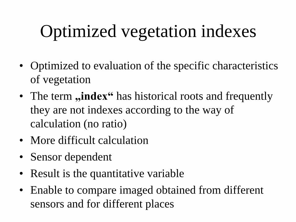
Optimized vegetation indexes
• Optimized to evaluation of the specific characteristics
of vegetation
• The term „index“ has historical roots and frequently
they are not indexes according to the way of
calculation (no ratio)
• More difficult calculation
• Sensor dependent
• Result is the quantitative variable
• Enable to compare imaged obtained from different
sensors and for different places

Slope-based vegetation indexes
• VI is based on the ratio R/NIR reflectancies which
create a semi-line from the axe origin (axes R and
NIR reflectance)

Slope-based VI
• ideally the slope of the line R-NIR should relate to
the quantity of vegetation
– β0 … free soil
– β1 … free soil, traces of vegetation
– β2 … soil dominates + vegetation occurence
– ……
– β6 … full coverage of vegetation

Ratio-based VI
• Comparison of the reflectance in R and NIR
• Various modifications
• RATIO, NDVI, RVI, NRVI, TVI, CTVI, TTVI
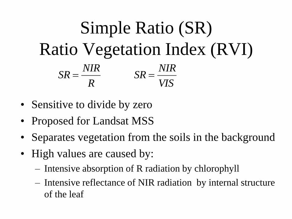
Simple Ratio (SR)
Ratio Vegetation Index (RVI)
• Sensitive to divide by zero
• Proposed for Landsat MSS
• Separates vegetation from the soils in the background
• High values are caused by:
– Intensive absorption of R radiation by chlorophyll
– Intensive reflectance of NIR radiation by internal structure
of the leaf
R
NIRSR
VIS
NIRSR

Normalized Differential Vegetation Index
NDVI
• Designed for Landsat MSS (1974), and other sensors
• Separates green vegetation from soils
• Higher values indicate massive occurence of vegetation
• Rich vegetation – positive values (0.3 - 0.8)
• Soils – small positive NDVI values (0.1 - 0.2).
• free standing water - very low positive or even slightly
negative NDVI values
• clouds and snow fields - negative values of NDVI
34
34
TMTM
TMTMNDVI
12
12
AVHRRAVHRR
AVHRRAVHRRNDVI

• NDVI in Europe.
Source: DLR

Transformed Vegetation Index TVI
• Designed as a modification of NDVI (1975)
• Express the quantity of green biomass
• Calibration required
• Partly eliminates the occurence of negative values
• linear development (normal distribution of data)
100*5,034
34
TMTM
TMTMTVI

Corrected Transformed Vegetation Index CTVI
• Proposed as a modification of TVI (1984)
• Eliminates disadvantages of NDVI and TVI caused by
negative values
• Disadvantage – overestimation of the green vegetation
occurrence

Thiam’s Transformed Vegetation Index TTVI
• navržen jako úprava CTVI (Thiam, 1999)
• eliminuje nedostatky CTVI způsobené nadhodnocováním
výskytu vegetace

Normalized Ratio Vegetation Index NRVI
• efekt normalizace se projevuje podobně jako u NDVI
– minimalizován problém variability osvětlení v důsledku
topografických vlivů
– lineární průběh stupnice
• omezuje negativní vliv atmosféry
• normální rozdělení hodnot NRVI

Orthogonal (distance-based) VI
• využívají linii půd - popisující charakteristické
příznaky odrazivosti půd pro R a NIR záření

Orthogonal (distance-based) VI
• pixely, reprezentující holé půdy, vykazují kladnou korelaci
hodnot odrazivosti pro R a NIR pásma
• výpočet rovnice linie půd metodou nejmenších čtverců

Perpendicular Vegetation Index PVI
• základ ortogonálních indexů
• z PVI odvozeny další vegetační indexy
• hlavní smyslem je:
– minimalizovat vliv míchání spektrální odezvy řídké
vegetace a půd v pozadí
– řeší problém smíšených pixelů
• použití v aridních a semi-aridních oblastech

Other (non-VI) indexes

Other (non-VI) indexes
• NDWI – normalised difference water index (vlhkost v
rostlinách), vyžadována pásma 900 a 1250 nm
• NDSI - normalised difference snow index – pásma 500 nm a
1500 nm
• NBR - normalised burn ratio – pásma 1000 nm a 2000 nm
• Hydrokarbonový index (Smejkalová)

© Dobrovolný

© Dobrovolný

© Dobrovolný

© Dobrovolný

© Dobrovolný

© Dobrovolný

• analýza hlavních komponent, dekorelační roztažení histogramu
http://web.natur.cuni.cz/ugp/main/staff/martinek/DPZda
ta/3-DPZ-ImageAnal.pdf

• PC1, PC2, PC3 jako RGB
• PC1, PC2, PC3 jako RGB – decorrelation a D-roztažení
http://web.natur.cuni.cz/ugp/main/staff/martinek/DPZda
ta/3-DPZ-ImageAnal.pdf

© Dobrovolný
© Dobrovolný

© Dobrovolný

© Kolář
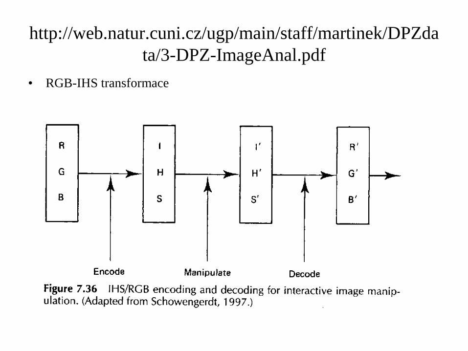
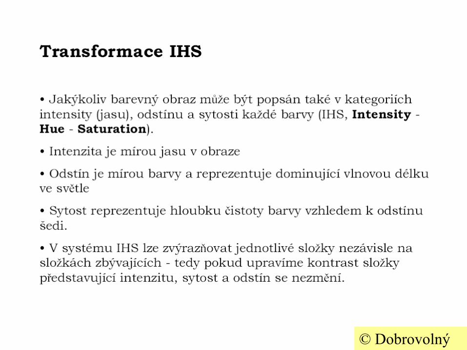
• RGB-IHS transformace
http://web.natur.cuni.cz/ugp/main/staff/martinek/DPZda
ta/3-DPZ-ImageAnal.pdf

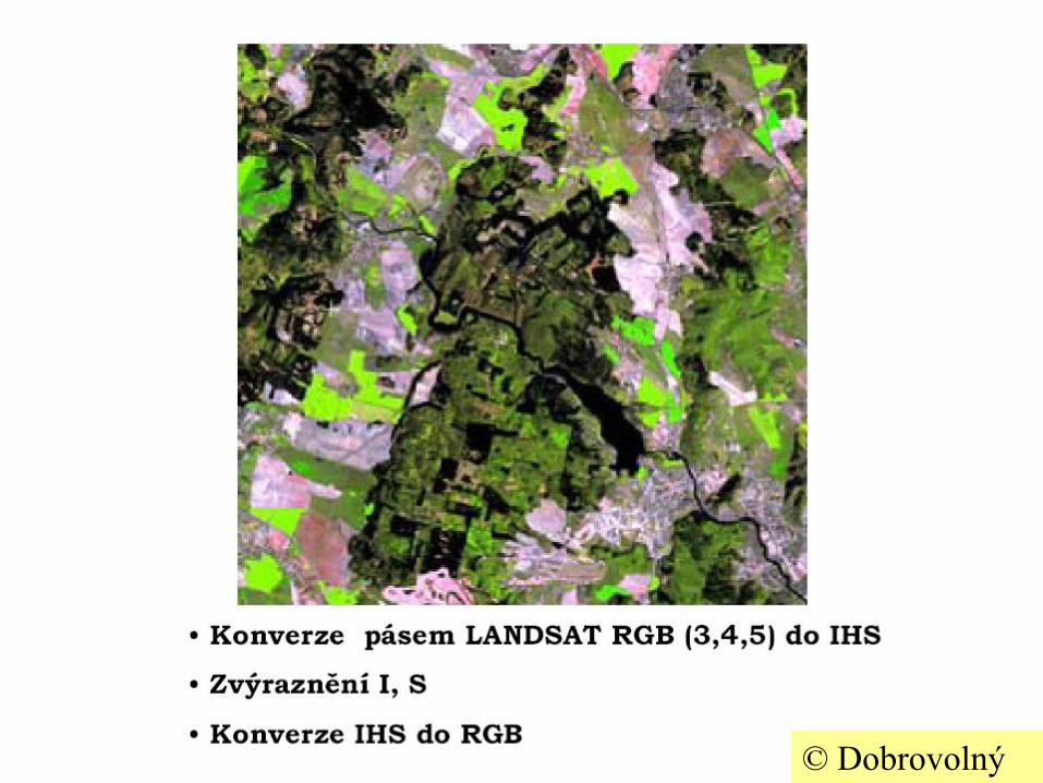
• RGB-IHS transformace
http://web.natur.cuni.cz/ugp/main/staff/martinek/DPZda
ta/3-DPZ-ImageAnal.pdf

© Dobrovolný

© Dobrovolný
© Dobrovolný

Resolution Merge
• spojení obrazů s různým rozlišením
• získání výsledného obrazu, který má prostorové a spektrální rozlišení stejné jako vyšší z obou původních vstupních obrazových záznamů
• např.:
– Landsat 7 - pásma 1-5, 7 prostorové rozlišení 30 m/pixel
– Landsat 7 - pásmo 8 prostorové rozlišení 15 m/pixel
• výsledkem tzv. PAN sharpened image

Resolution Merge

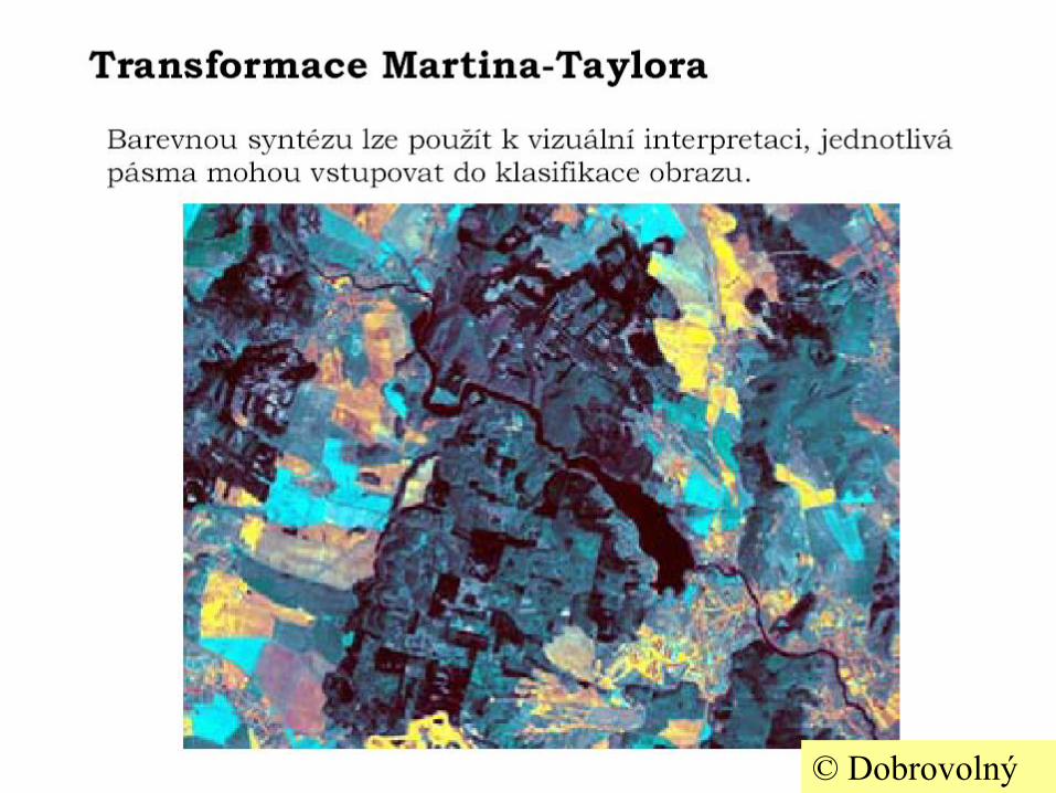
Jiné varianty využití RGB<->IHS
• Odlišení jemných změn v plochách hornin: • MSS4, MSS5, MSS7 do složky I;
• MSS5/MSS4 do H;
• MSS5/MSS6 do S;
• Pak zpětná transformace do RGB
• Podobně geologické struktury pro SEASAT
• Tvorba zavěšených map na reliéfu: • Obraz mapy do I;
• DMT do H;
• 127 do S;
• zpětná transformace do RGB
• Zvýraznění AVHRR (pouze 2 pásma). 1+2 = I; 2/1 do H; 1-2=S

• TM 5/4 3/1 5/7 jako RGB - HSI transformace
http://web.natur.cuni.cz/ugp/main/staff/martinek/DPZda
ta/3-DPZ-ImageAnal.pdf

Brovey transformation
• využívá 3 pásma multispektrálního obrazového záznamu +
obraz s vysokým prostorovým rozlišením
• např.:
[DNB1/ (DNB1+ DNB2+ DNB3)] x [DNHiResImage] = DNB1new
[DNB2/ (DNB1+ DNB2+ DNB3)] x [DNHiResImage] = DNB2new
[DNB3/ (DNB1+ DNB2+ DNB3)] x [DNHiResImage] = DNB3new
• usnadnění vizuální interpretace
• zvýšení kontrastu v oblast nejsvětlejších a nejtmavších
charakteristik (poskytuje kontrast ve stínech, v oblasti
vodních objektů, …)

© Dobrovolný
© Dobrovolný

M-T Transformation – merging
principal components
• využívá PC-1 pásmo – iluminace scény
• usnadnění vizuální interpretace
• zvýšení kontrastu v oblast nejsvětlejších a
nejtmavších charakteristik (poskytuje kontrast ve
stínech, v oblasti vodních objektů, …)

Literatura • Jackson, R. D. and Huete, A. R. (1991) Interpreting vegetation
indexes. Prev. Vet. Med. 11. pp. 185–200
• Dobrovolný P.: Dálkový průzkum Země. Digitální zpracování
obrazu. Brno 1998.
• http://www.chemagazin.cz/userdata/chemagazin_2010/file/CHE
MAGAZIN_XX_6_cl10%281%29.pdf
• IDRISI Manual, kap. 18 – Vegetation indices


![hoµ o f^v À ^v R] ]u] P] ]zfoWíU^ÇfWíU oflîìíôU Xíjiajournal.com/files/19b6deb0-d263-4517-a910-2803739d7786ss.pdf · DÜNYA 7>>m^dZdPZ> Z/ ARASINDA YERINI ALAN TÜRK SANATÇI](https://static.fdocuments.net/doc/165x107/5e123f073e3bf83d8c54c0fd/ho-o-fv-v-r-u-p-zfowufwu-oflu-x-doenya-7mdzdpz.jpg)