Dynamometer Cards
115
eProduction Solutions LOWIS User Course Beam Optimization Page 1 Dynamometer Cards (Surface and Downhole) Dynamometer Cards (Surface and Downhole) Surface Dynamometer Cards Webster defines a “dynamometer” as an instrument used to measure force. In terms of its use in the “oil patch”, a dynamometer records polished rod load in relation to polished rod position. The result is a plot of “load versus position” – commonly called the surface “dynamometer card” that measure the amount of work being done by the pumping system. Dynamometer systems allow the user to record the necessary information to generate a “surface card” – i.e., load and position data. This data can then be analyzed by any “wave equation” driven diagnostic program. Analysis results include downhole cards, load/stress calculations, counterbalance information, pump displacement, calculated fluid levels, estimated electrical costs, etc. Through the years, the polished rod dynamometer has been the principal tool for analyzing the operation of rod pumped wells. The shape of the surface dynamometer card is determined by changing downhole conditions. Ideally, these conditions would be apparent from the surface dynamometer card by visual interpretation. However, because of the complex behavior of the rod string and the great diversity of card shapes, visual diagnosis is not always possible. Though much information can be gained from visual interpretation of surface cards, success is directly linked to the skill and experience of the analyst – and even the most experienced analysts are often misled into an incorrect diagnosis. The graphic shown in the next slide illustrates how “surface card” shape relates to pump depth/size, SPM, stroke length, and rod diameter.
description
Levantamiento artificial Bombeo Mecánico
Transcript of Dynamometer Cards

eProduction Solutions LOWIS User CourseBeam OptimizationPage 1
Dynamometer Cards
(Surface and Downhole)
Dynamometer Cards (Surface and Downhole)
Surface Dynamometer Cards
Webster defines a “dynamometer” as an instrument used to measure force. In terms of its use in the “oil patch”, a dynamometer records polished rod load in relation to polished rod position. The result is a plot of “load versus position” – commonly called the surface “dynamometer card” that measure the amount of work being done by the pumping system. Dynamometer systems allow the user to record the necessary information to generate a “surface card” – i.e., load and position data. This data can then be analyzed by any “wave equation” driven diagnostic program. Analysis results include downhole cards, load/stress calculations, counterbalance information, pump displacement, calculated fluid levels, estimated electrical costs, etc. Through the years, the polished rod dynamometer has been the principal tool for analyzing the operation of rod pumped wells. The shape of the surface dynamometer card is determined by changing downhole conditions. Ideally, these conditions would be apparent from the surface dynamometer card by visual interpretation. However, because of the complex behavior of the rod string and the great diversity of card shapes, visual diagnosis is not always possible. Though much information can be gained from visual interpretation of surface cards, success is directly linked to the skill and experience of the analyst – and even the most experienced analysts are often misled into an incorrect diagnosis. The graphic shown in the next slide illustrates how “surface card” shape relates to pump depth/size, SPM, stroke length, and rod diameter.

eProduction Solutions LOWIS User CourseBeam OptimizationPage 2
Dynamometer Cards
(Surface and Downhole)
Polished Rod Load Points vs. Polished Rod Position Polished Rod Load Points vs. Polished Rod Position Points = Points = DynamometerDynamometer CardCard
The Way It The Way It Used To Be Used To Be ……

eProduction Solutions LOWIS User CourseBeam OptimizationPage 3
Dynamometer Cards
(Surface and Downhole)

eProduction Solutions LOWIS User CourseBeam OptimizationPage 4
Dynamometer Cards
(Surface and Downhole)
TodayToday’’s Load Input Devicess Load Input Devices
Position Input DevicesPosition Input Devices

eProduction Solutions LOWIS User CourseBeam OptimizationPage 5
Dynamometer Cards
(Surface and Downhole)
Raw Position and Load Values for Dynamometer Raw Position and Load Values for Dynamometer Card GenerationCard Generation
If these If these ““position pointsposition points”” are plotted against the are plotted against the ““load pointsload points”” –– what is the result?what is the result?
A surface dynamometer card A surface dynamometer card ……

eProduction Solutions LOWIS User CourseBeam OptimizationPage 6
Dynamometer Cards
(Surface and Downhole)

eProduction Solutions LOWIS User CourseBeam OptimizationPage 7
Dynamometer Cards
(Surface and Downhole)

eProduction Solutions LOWIS User CourseBeam OptimizationPage 8
Dynamometer Cards
(Surface and Downhole)

eProduction Solutions LOWIS User CourseBeam OptimizationPage 9
Dynamometer Cards
(Surface and Downhole)

eProduction Solutions LOWIS User CourseBeam OptimizationPage 10
Dynamometer Cards
(Surface and Downhole)
The following several slides are a library of “API 11L2”generated surface dynamometer cards and actual cards gathered in the field.

eProduction Solutions LOWIS User CourseBeam OptimizationPage 11
Dynamometer Cards
(Surface and Downhole)

eProduction Solutions LOWIS User CourseBeam OptimizationPage 12
Dynamometer Cards
(Surface and Downhole)

eProduction Solutions LOWIS User CourseBeam OptimizationPage 13
Dynamometer Cards
(Surface and Downhole)

eProduction Solutions LOWIS User CourseBeam OptimizationPage 14
Dynamometer Cards
(Surface and Downhole)

eProduction Solutions LOWIS User CourseBeam OptimizationPage 15
Dynamometer Cards
(Surface and Downhole)

eProduction Solutions LOWIS User CourseBeam OptimizationPage 16
Dynamometer Cards
(Surface and Downhole)

eProduction Solutions LOWIS User CourseBeam OptimizationPage 17
Dynamometer Cards
(Surface and Downhole)

eProduction Solutions LOWIS User CourseBeam OptimizationPage 18
Dynamometer Cards
(Surface and Downhole)

eProduction Solutions LOWIS User CourseBeam OptimizationPage 19
Dynamometer Cards
(Surface and Downhole)
Calculated Downhole Pump Card
Bottom Hole Analysis
In the studies of surface dynamometer cards, it is understood that one of the primary things that affect the shape of the actual dynamometer card is the load condition at the bottom of the hole. Therefore, bottomhole conditions such as crooked hole, paraffin,scale, sand, and solids all affect the loads and the shape of the card.In an effort to find out exactly what was happening at the bottom of the hole, W. E. Gilbert and others designed a bottomhole dynagraph that measured loads and displacements at the bottom of the hole. His work, and a number of bottomhole dynagraphs, was published in 1936. In 1967, Sam Gibbs received a patent on a mathematical method for simulating the sucker rod pumping system. His work and the work of others made it possibleto use a surface dynamometer card as a basis for a simulatedbottom hole card. In 1986 G. Albert designed an electronic bottomhole analyzer which measured the bottom hole conditions electronically in the same manner that W. E. Gilbert had measured them mechanically. This tool confirmed that the mathematical simulation from surface dynamometer cards does indeed give accurate bottomhole loads and displacements.

eProduction Solutions LOWIS User CourseBeam OptimizationPage 20
Dynamometer Cards
(Surface and Downhole)
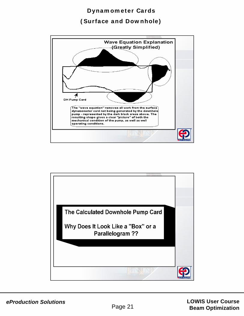
The mysterious "black magic" of an experienced surface card “dynamometer” analyst was and continues to be based on a lifetime of observation and experience. Today, with a thorough understanding of the principles involved and aided by computer simulation, an accurate analysis of the problem is possible in nearly every case.
To bridge the gap between interpretation of the surface card (“black magic”) and quantitative downhole data, today’s diagnostic programs make use of a mathematical solution based on a model of the rod pumping system, known throughout the industry as the “wave equation”. The resulting subsurface or downhole card removes personal judgment and experience from the diagnosis of downhole conditions.
eProduction Solutions LOWIS User CourseBeam OptimizationPage 21
Dynamometer Cards
(Surface and Downhole)

eProduction Solutions LOWIS User CourseBeam OptimizationPage 22
Dynamometer Cards
(Surface and Downhole)
Rod Pumping VisualizationFor Four of the Basic Downhole Pump Card Shapes
Net Pump Stroke (in.)
Load
(Lbs
)Full Pump
Load
(Lbs
) Gas Interference
orCompression Lo
ad (L
bs)
Tubing Movement
Load
(Lbs
)
Pump-Off
Click Anywhere to Continue0.2
Net Pump Stroke (in.)
Net Pump Stroke (in.)Net Pump Stroke (in.)
Rod Pumping Visualization
Traveling Valve
Standing Valve
Downhole Pump card
Pump Stroke (Inches)
Load
(Lbs
)
Pressure Above
Plunger
Pressure Below
Plunger
Click Anywhere to Continue
Tubing Anchor
Full Pump
Fluid Load On Plunger
Ball
Seat
Pump Plunger
Pump Barrel
Maximum Fluid Load
Minimum Fluid Load
Top of Stroke
F1-03
Fluid Level
PumpHold-Down
Rod String
Tubing
Casing
Polished rod in the hole – bottom of strokeBall
Seat

eProduction Solutions LOWIS User CourseBeam OptimizationPage 23
Dynamometer Cards
(Surface and Downhole)
Start of Upstroke
Net Stroke (in.)
Load
(Lbs
)SV Open – Rods Support Fluid Column (load increases)SV Closed – Tubing Supports Fluid Column (load)
Pressure Above
Plunger
Pressure Below
Plunger
Tubing Anchor
TV Closed (loads increase to maximum)
Click Anywhere to ContinueF2-04
Upstroke Completed
Net Stroke (in.)
Load
(Lbs
)
SV Open – Rods Support Fluid Column (load)
Pressure Above
Plunger
Pressure Below
Plunger
Click Anywhere to Continue
Tubing Anchor
TV Closed (load @ maximum)
F3-05
Pump moves up the hole

eProduction Solutions LOWIS User CourseBeam OptimizationPage 24
Dynamometer Cards
(Surface and Downhole)
Downstroke Begins
SV Open – Rods Support Fluid ColumnSV Will Close – Tubing Supports Fluid Column (load)
Net Stroke (in.)
Load
(Lbs
)
Pressure Above
Plunger
Pressure Below
Plunger
Click Anywhere to Continue
Tubing Anchor
TV ClosedTV Will Open (loads decrease)
F4-06
Pump Downstroke Completes
SV Closed – Tubing Supports Fluid Column (load)
Net Stroke (in.)
Load
(Lbs
)
TV Open(loads @ minimum)
Pressure Above
Plunger
Pressure Below
Plunger
Click Anywhere to Continue
Tubing Anchor
F5-07
Pump moves down

eProduction Solutions LOWIS User CourseBeam OptimizationPage 25
Dynamometer Cards
(Surface and Downhole)
Pump Stroke Complete
SV Closed – Tubing Supports Fluid Column (load)
Net Stroke (in.)
Load
(Lbs
)
TV OpenTV Will Close
Pressure Above
Plunger
Pressure Below
Plunger
Click Anywhere to Continue
Tubing Anchor
F6-08
Full Downhole Pump Card
Rod Pumping Visualization
Traveling Valve
Standing Valve
Net Stroke (in.)
Load
(Lbs
)
Pressure Above
Plunger
Pressure Below
Plunger
Click Anywhere to Continue
Tubing Anchor Gas
Interference(high pressure gas)
Downhole Pump Card
G1-09
Fluid Level

eProduction Solutions LOWIS User CourseBeam OptimizationPage 26
Dynamometer Cards
(Surface and Downhole)
Start of Upstroke
TV Closed(loads increase to maximum)
Net Stroke (in.)
Load
(Lbs
)SV Open – Rods Support Fluid Column (load increases)SV Closed – Tubing Supports Fluid Column (load)
Pressure Above
Plunger
Pressure Below
Plunger
Click Anywhere to Continue
Tubing Anchor
G2-10
Fluid Level
Pump Upstroke Completes
Net Stroke (in.)
Load
(Lbs
)
SV Open – Rods Support Fluid Column (load)
TV Closed
Pressure Above
Plunger
Pressure Below
Plunger
Click Anywhere to Continue
Tubing Anchor
G3-11
Fluid Level
Pump moves up the hole

eProduction Solutions LOWIS User CourseBeam OptimizationPage 27
Dynamometer Cards
(Surface and Downhole)
Start of Downstroke
TV Closed
SV Open – Rods Support Fluid Column (load)SV Will Close – Tubing Supports Fluid Column (load)
Net Stroke (in.)
Load
(Lbs
)
Pressure Above
Plunger
Pressure Below
Plunger
Click Anywhere to Continue
Tubing Anchor
G4-12
Gas below pump must be compressed before traveling valve can open
Fluid Level
Downstroke (cont.)
TV ClosedTV Will Open(loads decrease)
SV Closed – Tubing Supports Fluid Column (load)
Net Stroke (in.)
Load
(Lbs
)
Pressure Above
Plunger
Pressure Below
Plunger
Click Anywhere to Continue
Tubing Anchor
G5-13
Fluid Level
Gas CompressionComplete
eProduction Solutions LOWIS User CourseBeam OptimizationPage 28
Dynamometer Cards
(Surface and Downhole)
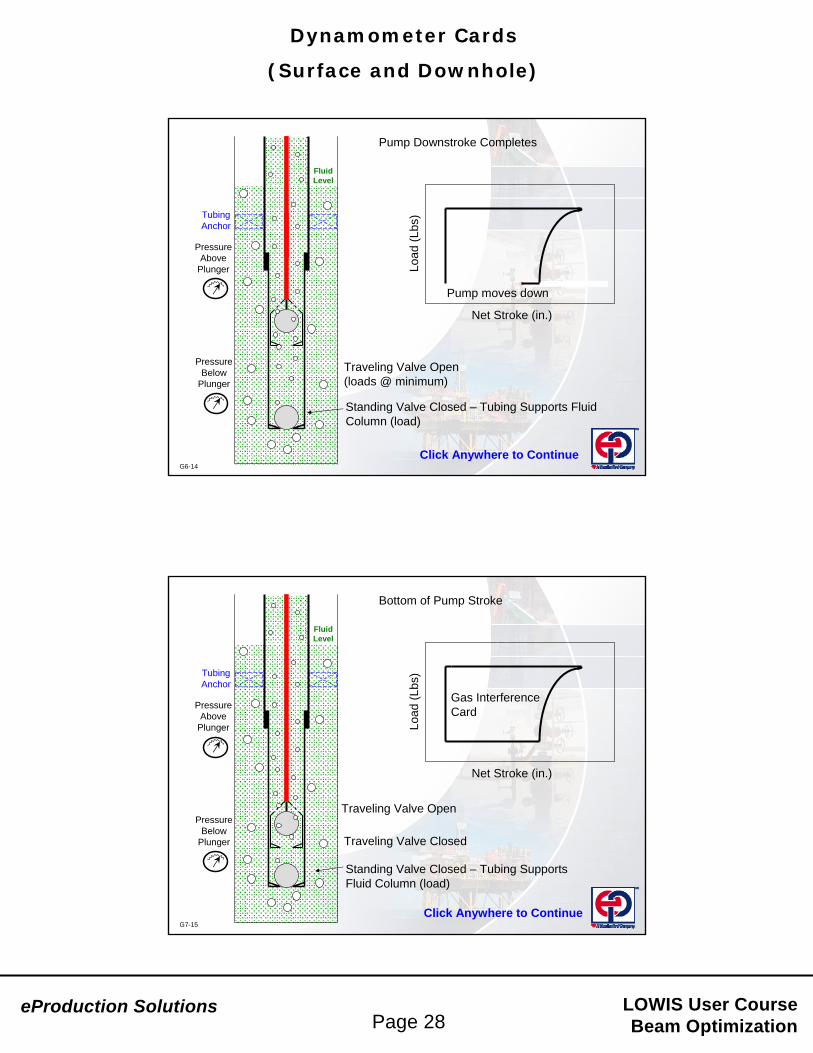
Pump Downstroke Completes
Standing Valve Closed – Tubing Supports Fluid Column (load)
Net Stroke (in.)
Load
(Lbs
)
Traveling Valve Open(loads @ minimum)
Pressure Above
Plunger
Pressure Below
Plunger
Click Anywhere to Continue
Tubing Anchor
G6-14
Fluid Level
Pump moves down
Bottom of Pump Stroke
Traveling Valve Closed
Standing Valve Closed – Tubing Supports Fluid Column (load)
Net Stroke (in.)
Load
(Lbs
)
Traveling Valve Open
Pressure Above
Plunger
Pressure Below
Plunger
Click Anywhere to Continue
Tubing Anchor
G7-15
Fluid Level
Gas InterferenceCard

eProduction Solutions LOWIS User CourseBeam OptimizationPage 29
Dynamometer Cards
(Surface and Downhole)
Rod Pump Visualization
Traveling Valve
Standing Valve
Net Stroke (in.)
Load
(Lbs
)
Pressure Above
Plunger
Pressure Below
Plunger
Click Anywhere to Continue
Tubing Anchor
Pump-Off(low pressure gas)
Downhole Pump Card
O1-16
Fluid Level
Start of Upstroke
Traveling Valve Closed (load increases to maximum)
Standing Valve Closed – Tubing Supports Fluid Column (load)
Net Stroke (in.)
Load
(Lbs
)
Standing Valve Will Open – Rods Support Fluid Column
Pressure Above
Plunger
Pressure Below
Plunger
Click Anywhere to Continue
Tubing Anchor
O2-17
Fluid Level
eProduction Solutions LOWIS User CourseBeam OptimizationPage 30
Dynamometer Cards
(Surface and Downhole)
Low Pressure
Gas
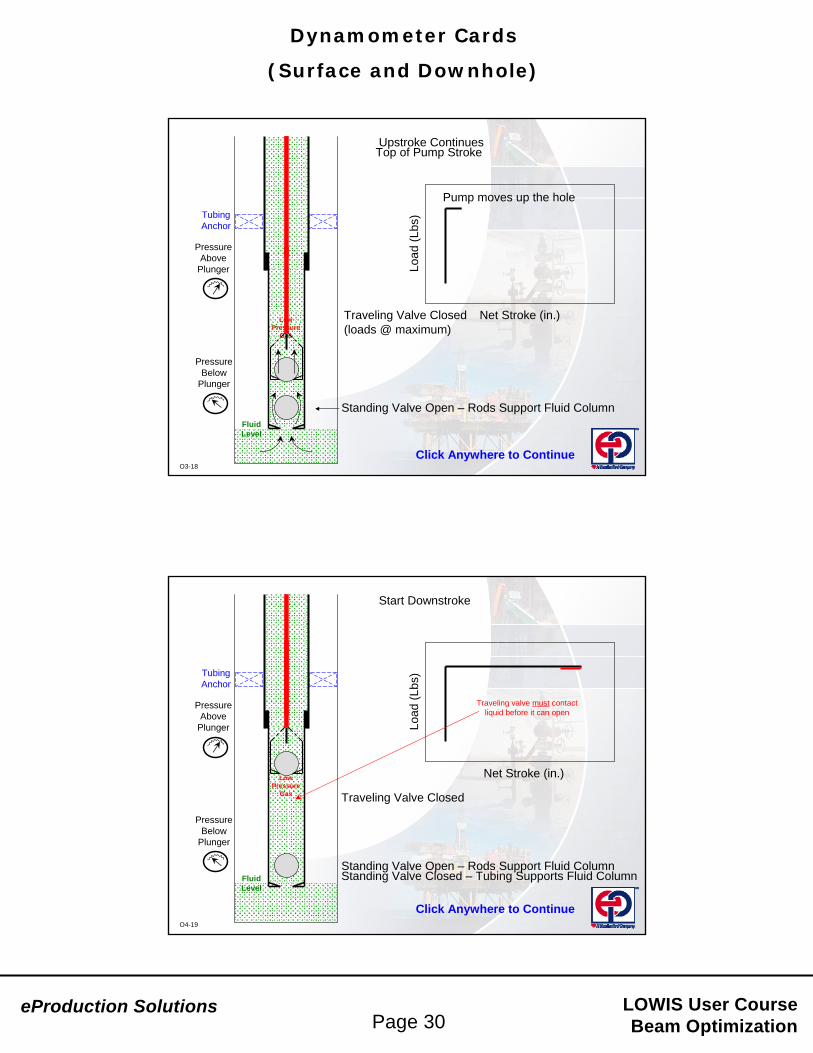
Upstroke Continues
Net Stroke (in.)
Load
(Lbs
)Standing Valve Open – Rods Support Fluid Column
Traveling Valve Closed(loads @ maximum)
Top of Pump Stroke
Pressure Above
Plunger
Pressure Below
Plunger
Click Anywhere to Continue
Tubing Anchor
O3-18
Fluid Level
Pump moves up the hole
Start Downstroke
Traveling Valve Closed
Standing Valve Open – Rods Support Fluid ColumnStanding Valve Closed – Tubing Supports Fluid Column
Net Stroke (in.)
Load
(Lbs
)
Pressure Above
Plunger
Pressure Below
Plunger
Click Anywhere to Continue
Tubing Anchor
O4-19
Low Pressure
Gas
Traveling valve must contact liquid before it can open
Fluid Level

eProduction Solutions LOWIS User CourseBeam OptimizationPage 31
Dynamometer Cards
(Surface and Downhole)
Downstroke (cont.)
Traveling Valve Closed
Standing Valve Closed – Tubing Supports Fluid Column
Net Stroke (in.)
Load
(Lbs
)
Traveling Valve Open(loads to minimum)
Pressure Above
Plunger
Pressure Below
Plunger
Click Anywhere to Continue
Tubing Anchor
O5-20
Traveling valve opens late in the downstroke
Fluid Level
Pump Downstroke Completes
Standing Valve Closed – Tubing Supports Fluid Column
Net Stroke (in.)
Load
(Lbs
)
Traveling Valve Open(loads @ minimum)
Pressure Above
Plunger
Pressure Below
Plunger
Click Anywhere to Continue
Tubing Anchor
O6-21
Fluid Level
eProduction Solutions LOWIS User CourseBeam OptimizationPage 32
Dynamometer Cards
(Surface and Downhole)
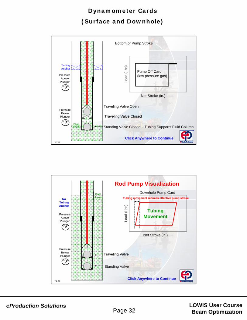
Bottom of Pump Stroke
Traveling Valve Closed
Standing Valve Closed – Tubing Supports Fluid Column
Net Stroke (in.)
Load
(Lbs
)
Traveling Valve Open
Pressure Above
Plunger
Pressure Below
Plunger
Click Anywhere to Continue
Tubing Anchor
O7-22
Fluid Level
Pump Off Card(low pressure gas)
Rod Pump Visualization
Traveling Valve
Standing Valve
Net Stroke (in.)
Load
(Lbs
)
Pressure Above
Plunger
Pressure Below
Plunger
Click Anywhere to Continue
No Tubing Anchor
Tubing Movement
Downhole Pump Card
T1-23
Tubing movement reduces effective pump strokeFluid Level

eProduction Solutions LOWIS User CourseBeam OptimizationPage 33
Dynamometer Cards
(Surface and Downhole)
Start of Upstroke
Traveling Valve Closed(loads to maximum)
Standing Valve Closed – Tubing Supports Fluid Column
Net Stroke (in.)
Load
(Lbs
)
Pressure Above
Plunger
Pressure Below
Plunger
Click Anywhere to Continue
No Tubing Anchor
T2-24
Tubing moves up due to rods now supporting the fluid load
Lost effective pump stroke
Upstroke Continues
Net Stroke (in.)
Load
(Lbs
)
Standing Valve Open – Rods Support Fluid Column
Traveling Valve Closed(loads @ maximum)
Top of Pump Stroke
Pressure Above
Plunger
Pressure Below
Plunger
Click Anywhere to Continue
No Tubing Anchor
Standing Valve Closed – Tubing Supports Fluid Column
T3-25
Pump moves up the hole

eProduction Solutions LOWIS User CourseBeam OptimizationPage 34
Dynamometer Cards
(Surface and Downhole)
Start Downstroke
Traveling Valve Closed
Standing Valve Open – Rods Support Fluid ColumnStanding Valve Closed – Tubing Supports Fluid Column
Net Stroke (in.)
Load
(Lbs
)
Pressure Above
Plunger
Pressure Below
Plunger
Click Anywhere to Continue
No Tubing Anchor
T4-26
Downstroke (cont.)
Traveling Valve Closed
Standing Valve Open – Rods Support Fluid ColumnStanding Valve Closed – Tubing Supports Fluid Column
Net Stroke (in.)
Load
(Lbs
)
Pressure Above
Plunger
Pressure Below
Plunger
Click Anywhere to Continue
No Tubing Anchor
Traveling Valve Open(loads decrease to minimum)
T5-27
Tubing moves down due to rods no longer supporting the fluid load

eProduction Solutions LOWIS User CourseBeam OptimizationPage 35
Dynamometer Cards
(Surface and Downhole)
Downstroke Completes
Standing Valve Closed – Tubing Supports Fluid Column
Net Stroke (in.)
Load
(Lbs
)
Traveling Valve Open(loads @ minimum)
Pressure Above
Plunger
Pressure Below
Plunger
Click Anywhere to Continue
No Tubing Anchor
T6-28
Pump moves down
Bottom of pump Stroke
Traveling Valve Closed
Standing Valve Closed – Tubing Supports Fluid Column
Net Stroke (in.)
Load
(Lbs
)
Traveling Valve Open
Pressure Above
Plunger
Pressure Below
Plunger
Click Anywhere to Continue
No Tubing Anchor
T7-29
Tubing MovementCard

eProduction Solutions LOWIS User CourseBeam OptimizationPage 36
Dynamometer Cards
(Surface and Downhole)
The following several slides show example calculated downhole pump cards and explanations that are the result of the “wave equation” diagnostic solution.
The shape of a downhole pump card showing full liquid fillage (with anchored tubing) is approximately rectangular.

eProduction Solutions LOWIS User CourseBeam OptimizationPage 37
Dynamometer Cards
(Surface and Downhole)
Detailed Description
1. At point “A”, the traveling valve closes and the load begins to be transferred from the tubing to the rods.
2. Between points “A” and “B”, tension in the pull rod is increasing as the rods are picking up the fluid.
3. At point “B”, the entire fluid load is borne by the rods and the standing valve opens.
4. Between points “B” and “C”, fluid is being lifted toward the surface. At the same time, the pump chamber below the traveling valve is filling completely with liquid through the open standing valve.
5. At point “C”, the top of the stroke has been reached and the downward tendency of the pump motion causes the standing valve to close.
6. Between points “C” and “D”, the fluid load is being transferred back to the tubing. Because the pump chamber has filled completely with liquid (nearly incompressible) the pump cannot move downward until the entire fluid load has been released. This is one of the reasons for the rectangular card shape. The pump remains stationary (if the tubing is anchored) while the load is being transferred back to the tubing from the rods.
7. At point “D”, the traveling valve opens and the pump begins to descend. 8. Between points “D” and “A”, the pump descends with the traveling valve open (standing valve closed) through the fluid that entered the pump chamber during the upstroke.
9. At point “A”, the traveling valve is closed by the tendency of the pump to move upward. This action begins another pumping cycle.
Important Conclusion When a pump fills completely with liquid (with anchored tubing), traveling and standing valve actuation occurs at the top and bottom of the stroke with little movement of the pump. This gives the downhole pump card a characteristic rectangular appearance.

eProduction Solutions LOWIS User CourseBeam OptimizationPage 38
Dynamometer Cards
(Surface and Downhole)
A downhole pump card with unanchored tubing (full liquid fillage) has a parallelogram shape. The amount of tubing movement (in inches) can be scaled off from the downhole card to determine the amount of pump displacement being lost to unanchored tubing.
Detailed Description
1. At point “A”, the traveling valve closes and the load begins to be transferred from the tubing to the rods.
2. Between points “A” and “B”, tension in the pull rod is increasing as the rods are picking up the fluid. The pump is moving relative to the casing as the fluid load is being picked up. The pump is stationary relative to the tubing. Since the tubing is not anchored, the tubing shortens as the load is removed from it. Because the pump is riding along with the tubing, the pump moves relative to the casing. This movement can be detected with the use of the “wave equation” diagnostic solution. The horizontal distance between points “A” and “B” is the amount of tubing “stretch” in inches.
3. At point “B”, the entire fluid load is borne by the rods and the standing valve opens.
4. Between points “B” and “C”, fluid is being lifted toward the surface. At the same time, the pump chamber below the traveling valve is filling completely with liquid through the open standing valve.
5. At point “C”, the top of the stroke has been reached and the downward tendency of the pump motion causes the standing valve to close.
6. Between points “C” and “D”, the pump load is transferred from the rods to the tubing. As the load shifts to the tubing, the tubing stretches downward relative to the casing. Thus, pump movement relative to the casing can be detected by the “wave equation” diagnostic solution.
7. At point “C”, the traveling valve opens and the pump begins to descend.8. Between points “D” and “A”, the pump descends with the traveling valve open
(standing valve closed) through the fluid that entered the pump chamber during the upstroke.
9. At point “A”, the traveling valve is closed by the tendency of the pump to move upward. This action begins another pumping cycle.

eProduction Solutions LOWIS User CourseBeam OptimizationPage 39
Dynamometer Cards
(Surface and Downhole)

eProduction Solutions LOWIS User CourseBeam OptimizationPage 40
Dynamometer Cards
(Surface and Downhole)
The shape of a downhole pump card with gas interference shows a gas compression curve in the upper portion of the downstroke (points “C” - “D”).
Detailed Description
1. At point “A”, the traveling valve closes and the load begins to be transferred from the tubing to the rods.
2. Between points “A” and “B”, tension in the pull rod is increasing as the rods are picking up the fluid. If the fluid in the lower portion of the pump chamber is compressible (very gassy), a slight upward movement of the pump may occur during the load pick-up.
3. At point “B”, the entire fluid load is borne by the rods and the standing valve opens.
4. Between points “B” and “C”, fluid is being lifted to the surface. At the same time, the pump chamber below the traveling valve is filling with a mixture of liquid and high-pressure gas through the open standing valve.
5. At point “C”, the top of the stroke has been reached and the downward tendency of the pump causes the standing valve to close.
6. Between points “C” and “D”, the fluid load is being transferred back to the tubing. Because of the compressible gas that entered the pump during the charging cycle, the load transfer takes place along a “compression curve”. The pump moves downward during load transfer – which compresses the gas in the chamber below the closed traveling valve. As the pressure in the gas below the traveling valve increases, the load is removed from the rods.
7. At point “D”, the pressure in the compressed gas in the pump chamber is high enough to offset the pressure in the tubing at which point the traveling valve opens. The pump continues to descend.
8. Between points “D” and “A”, the pump descends with the traveling valve open (standing valve closed) through the fluid that entered the pump chamber during the upstroke.
9. At point “A”, the traveling valve is closed by the tendency of the pump to move upward. This action begins another pumping cycle.

eProduction Solutions LOWIS User CourseBeam OptimizationPage 41
Dynamometer Cards
(Surface and Downhole)
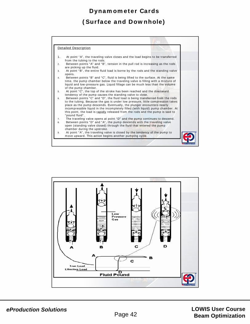
Fluid pound is a limiting case of gas interference. Pump intake pressure is low and the incompletely filled (with liquid) pump contains almost incompressible fluid. The load release thus takes place more abruptly than the gradual transfer that occurs with gas interference does.
eProduction Solutions LOWIS User CourseBeam OptimizationPage 42
Dynamometer Cards
(Surface and Downhole)
Detailed Description
1. At point “A”, the traveling valve closes and the load begins to be transferred from the tubing to the rods.
2. Between points “A” and “B”, tension in the pull rod is increasing as the rods are picking up the fluid.
3. At point “B”, the entire fluid load is borne by the rods and the standing valve opens.
4. Between points “B” and “C”, fluid is being lifted to the surface. At the same time, the pump chamber below the traveling valve is filling with a mixture of liquid and low-pressure gas. Liquid fillage can be much less than the volume of the pump chamber.
5. At point “C”, the top of the stroke has been reached and the downward tendency of the pump causes the standing valve to close.
6. Between points “C” and “D”, the fluid load is being transferred from the rods to the tubing. Because the gas is under low pressure, little compression takes place as the pump descends. Eventually, the plunger encounters nearly incompressible liquid in the incompletely filled (with liquid) pump chamber. At this point, the load is rapidly released from the rods and the pump is said to “pound fluid”.
7. The traveling valve opens at point “D” and the pump continues to descend.8. Between points “D” and “A”, the pump descends with the traveling valve
open (standing valve closed) through the fluid that entered the pump chamber during the upstroke.
9. At point “A”, the traveling valve is closed by the tendency of the pump to move upward. This action begins another pumping cycle.

eProduction Solutions LOWIS User CourseBeam OptimizationPage 43
Dynamometer Cards
(Surface and Downhole)
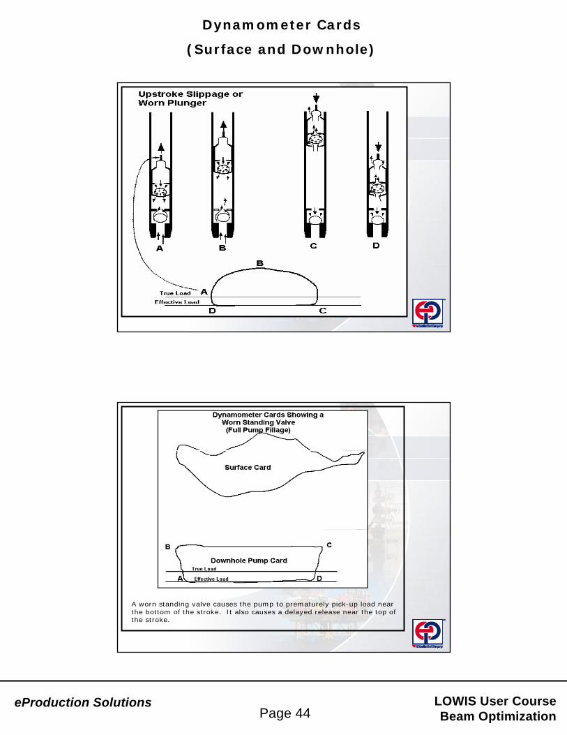
A worn traveling valve or plunger causes the pump to pick up the fluid load slowly at the bottom of the stroke and to release it prematurely at the top of the stroke.
Detailed Description
1. At point “A”, the traveling valve closes and the load begins to be transferred from the tubing to the rods.
2. Between points “A” and “B”, tension in the pull rod is increasing as the rods are picking up the fluid. The pump is moving slowly during this part of the cycle – thus its displacement rate is low. The pump slippage rate is a sizeable portion of the displacement rate. This causes the fluid load pick-up to be more gradual than usual.
3. At point “B”, the entire fluid load is borne by the rods and the standing valve opens.
4. Between points “B” and “C”, fluid is being lifted toward the surface. At the same time, the pump chamber below the traveling valve is filling completely with liquid through the open standing valve. In addition to this, fluids are slipping back around the worn traveling valve or plunger into the chamber below. This subtracts from the volume available for entry of new fluids from the reservoir.
5. At point “C”, the pump speed has again slowed down enough so that the slippage rate exceeds the displacement rate of the pump. This closes the standing valve. In a worn pump of this type, the load release begins prematurely near the top of the stroke.
6. Between points “C” and “D”, the fluid load is being transferred back to the tubing. The load is released with the pump still moving upward because of slippage. This happens because the slippage rate exceeds the pump displacement rate in this portion of the stroke.
7. At point “D”, the traveling valve opens and the pump begins to descend.8. Between points “D” and “A”, the pump descends with the traveling valve
open (standing valve closed) through the fluid that entered the pump chamber during the upstroke.
9. At point “A”, the traveling valve is closed by the tendency of the pump to move upward. This action begins another pumping cycle.
eProduction Solutions LOWIS User CourseBeam OptimizationPage 44
Dynamometer Cards
(Surface and Downhole)
A worn standing valve causes the pump to prematurely pick-up load near the bottom of the stroke. It also causes a delayed release near the top of the stroke.

eProduction Solutions LOWIS User CourseBeam OptimizationPage 45
Dynamometer Cards
(Surface and Downhole)
Detailed Description 1. At point “A”, the traveling valve closes and the load begins to be transferred from the
tubing to the rods. The load transfer begins with the pump still on the downstroke. This happens because the slippage rate past the standing valve exceeds the displacement rate of the slowly moving pump as it approaches the bottom of the stroke. This closes the traveling valve while the pump is still moving downward.
2. Between points “A” and “B”, tension in the pull rod is increasing as the rods are picking up the fluid.
3. At point “B”, the entire fluid load is borne by the rods and the standing valve opens. When the standing valve opens, slippage ceases.
4. Between points “B” and “C”, fluid is being lifted toward the surface. 5. At point “C”, the top of the stroke has been reached and the downward tendency of the
pump causes the standing valve to close. 6. Between points “C” and “D”, the fluid load is being transferred back to the tubing. The
load can be released with the pump moving down – even with complete liquid fillage. This can happen because slippage past the standing valve exceeds the displacement rate of the slowly moving pump.
7. At point “D”, the displacement rate of the pump exceeds the slippage rate of the standing valve and the traveling valve opens. The pump continues downward.
8. Between points “D” and “A”, the pump descends with the traveling valve open (standing valve closed) through the fluid that entered the pump chamber during the upstroke. Slippage past the standing valve is occurring – which decreases volumetric efficiency.
9. At point “A”, the pump has slowed down enough so that the slippage rate past the standing valve exceeds the displacement rate of the pump. This closes the traveling valve and a new pump cycle begins.

eProduction Solutions LOWIS User CourseBeam OptimizationPage 46
Dynamometer Cards
(Surface and Downhole)
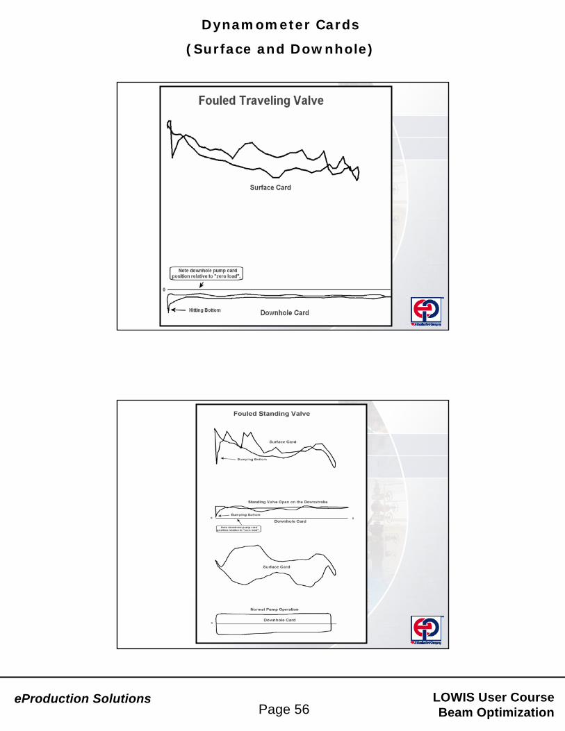
Pumps can “hit” up or down or both. This “hitting” or “bumping” condition can occur for any downhole situation – gas interference, fluid pound, unanchored tubing, etc. The case shown above has full liquid fillage.
If the pump “hits” down, a load loss (compression) will be shown at the lower left of the downhole card (at the bottom of the stroke on the downhole pump card).
If the pump “hits” up, a load increase (tension) will be shown at the top of the stroke (upper right on the downhole pump card).
Pumps that are identified as “hitting” up or down should be “re-spaced” to prevent equipment damage.

eProduction Solutions LOWIS User CourseBeam OptimizationPage 47
Dynamometer Cards
(Surface and Downhole)
Detailed Description
1. At point “A”, the plunger is below the bent section and the load on the pull rod is the same as for a full pump.
2. At point “B”, as the plunger reaches the “bend”, the load on the pull rod increases because the plunger must “squeeze” by this portion of the pump barrel.
3. At point “C”, the load reaches a maximum value and then decreases as the plunger moves away from the bend.
4. On the downstroke, the load on the pull rod is normal until the plunger reaches the “bad” spot in the barrel at point “E”.
5. The load on the pull rod decreases until the plunger reaches point “F”.
6. The pull rod load returns to normal after the plunger moves away from the bent portion of the pump barrel.

eProduction Solutions LOWIS User CourseBeam OptimizationPage 48
Dynamometer Cards
(Surface and Downhole)
Detailed Description
1. At point “A”, the plunger is below the bent section and the load on the pull rod is the same as for a full pump. 2. At point “B”, as the plunger reaches the “bend”, the load on the pull rod increases because the plunger must “squeeze” by this portion of the pump barrel. 3. At point “C”, the load reaches a maximum value and then decreases as the plunger moves away from the bend.4. On the downstroke, the load on the pull rod is normal until the plunger reaches the “bad” spot in the barrel at point “E”.5. The load on the pull rod decreases until the plunger reaches point “F”.6. The pull rod load returns to normal after the plunger moves away from the bent portion of the pump barrel.
eProduction Solutions LOWIS User CourseBeam OptimizationPage 49
Dynamometer Cards
(Surface and Downhole)
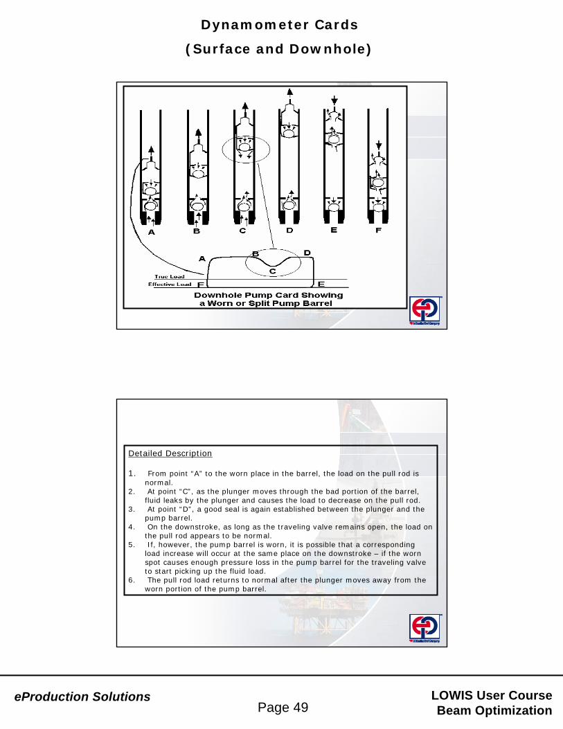
Detailed Description
1. From point “A” to the worn place in the barrel, the load on the pull rod is normal.
2. At point “C”, as the plunger moves through the bad portion of the barrel, fluid leaks by the plunger and causes the load to decrease on the pull rod.
3. At point “D”, a good seal is again established between the plunger and the pump barrel.
4. On the downstroke, as long as the traveling valve remains open, the load on the pull rod appears to be normal.
5. If, however, the pump barrel is worn, it is possible that a corresponding load increase will occur at the same place on the downstroke – if the worn spot causes enough pressure loss in the pump barrel for the traveling valve to start picking up the fluid load.
6. The pull rod load returns to normal after the plunger moves away from the worn portion of the pump barrel.

eProduction Solutions LOWIS User CourseBeam OptimizationPage 50
Dynamometer Cards
(Surface and Downhole)
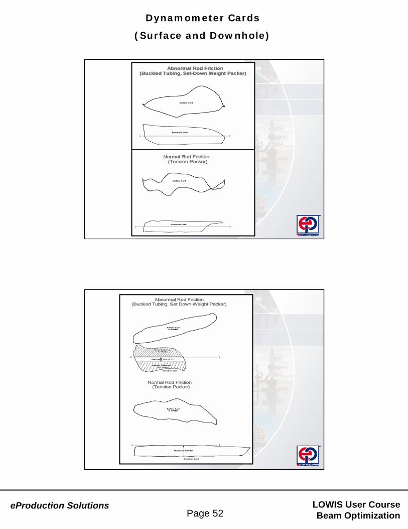
The graphic shown above helps to explain the downhole pump card shape for a full pump experiencing upstroke fluid inertia effects. This card shape is representative of wells with large plungers, of shallow depth (usually less than 4000’), and a high water cut.
Detailed Description
1. From points “A” to “B”, the inertia of the fluid in the tubing causes the load on the pull rod to increase as the plunger moves on the upstroke and “accelerates” the fluid above it.
2. At point “B”, the load on the pull rod reaches a maximum value.3. Between points “B” and “C”, the pressure “pulse” travels up the fluid
column and the pull rod drops – until the pressure “pulse” travels up the tubing and reflects back down. When this “reflected” wave reaches the plunger, it increases the pull rod load, but not as much as before.
4. The pull rod load returns to normal, assuming no further reflected “pulses” are seen by the plunger.

eProduction Solutions LOWIS User CourseBeam OptimizationPage 51
Dynamometer Cards
(Surface and Downhole)
More Downhole Pump Card Examples
Combinations of the following conditions can occur simultaneously.
eProduction Solutions LOWIS User CourseBeam OptimizationPage 52
Dynamometer Cards
(Surface and Downhole)

eProduction Solutions LOWIS User CourseBeam OptimizationPage 53
Dynamometer Cards
(Surface and Downhole)

eProduction Solutions LOWIS User CourseBeam OptimizationPage 54
Dynamometer Cards
(Surface and Downhole)

eProduction Solutions LOWIS User CourseBeam OptimizationPage 55
Dynamometer Cards
(Surface and Downhole)
eProduction Solutions LOWIS User CourseBeam OptimizationPage 56
Dynamometer Cards
(Surface and Downhole)

eProduction Solutions LOWIS User CourseBeam OptimizationPage 57
Dynamometer Cards
(Surface and Downhole)

eProduction Solutions LOWIS User CourseBeam OptimizationPage 58
Dynamometer Cards
(Surface and Downhole)

eProduction Solutions LOWIS User CourseBeam OptimizationPage 59
Dynamometer Cards
(Surface and Downhole)

eProduction Solutions LOWIS User CourseBeam OptimizationPage 60
Dynamometer Cards
(Surface and Downhole)

eProduction Solutions LOWIS User CourseBeam OptimizationPage 61
Dynamometer Cards
(Surface and Downhole)

eProduction Solutions LOWIS User CourseBeam OptimizationPage 62
Dynamometer Cards
(Surface and Downhole)

eProduction Solutions LOWIS User CourseBeam OptimizationPage 63
Dynamometer Cards
(Surface and Downhole)

eProduction Solutions LOWIS User CourseBeam OptimizationPage 64
Dynamometer Cards
(Surface and Downhole)
Things That Affect Calculated Downhole Pump Cards
Rod String Information:
Too short - Too long - Wrong length per rod - Wrong taper length – Wrong weight per foot – Wrong “Modulus of Elasticity” – Wrong “Speed of Sound” -
The examples shown in this slide and the next show what can happen to the calculated downhole pump card when input data is incorrect.
This example shows the downhole pump card shifted up and with a different shape as a result of an incorrect number of rods in each taper of a three taper rod string.

eProduction Solutions LOWIS User CourseBeam OptimizationPage 65
Dynamometer Cards
(Surface and Downhole)
The example above shows what happens to the downhole pump card when the “weight per foot” of each rod size is entered incorrectly in the database.

eProduction Solutions LOWIS User CourseBeam OptimizationPage 66
Dynamometer Cards
(Surface and Downhole)
Things That Affect Calculated Downhole Pump Cards
Incorrect Surface Loads
Strain gaugeBad calibrated load cell, load cable / connections
Poor Position Data
Position switch (TOS / Simulated Data Input)Bad “real position” device /cableImproper position device installation
• Damping Factor values control the amount of work from the surface dynamometer card that is applied to the calculated downhole pump card.
Increasing the “Damping Factors” results in smaller downhole cards/fluid loads.
Decreasing the “Damping Factors” results in larger downhole cards/fluid loads.
Note: Changing the “Damping Factors” is one way to help “model” conditions such as excessive friction or entrained gas.

eProduction Solutions LOWIS User CourseBeam OptimizationPage 67
Dynamometer Cards
(Surface and Downhole)
The example below also demonstrates the effects of increasing the “Damping Factors”:

eProduction Solutions LOWIS User CourseBeam OptimizationPage 68
Dynamometer Cards
(Surface and Downhole)
Class Exercise – Dynamometer Cards
Refer to the exercise handout. Record your observations in the space provided below each card or card pair.

eProduction Solutions LOWIS User CourseBeam OptimizationPage 69
Dynamometer Cards
(Surface and Downhole)
Extreme pump off (“gut pumped”) …
Bad pump off set-point? …
Restricted pump intake? ...
Pump off, gas compression ...

eProduction Solutions LOWIS User CourseBeam OptimizationPage 70
Dynamometer Cards
(Surface and Downhole)
Pumping unit “rolling” ...
Pumping unit “rolling” ...

eProduction Solutions LOWIS User CourseBeam OptimizationPage 71
Dynamometer Cards
(Surface and Downhole)
No pump valve action …
Tubing leak ?
TV not closing properly …
Possible “ring valve” pump ?

eProduction Solutions LOWIS User CourseBeam OptimizationPage 72
Dynamometer Cards
(Surface and Downhole)
Load cable short / connection? ...
SV hung open ...
eProduction Solutions LOWIS User CourseBeam OptimizationPage 73
Dynamometer Cards
(Surface and Downhole)
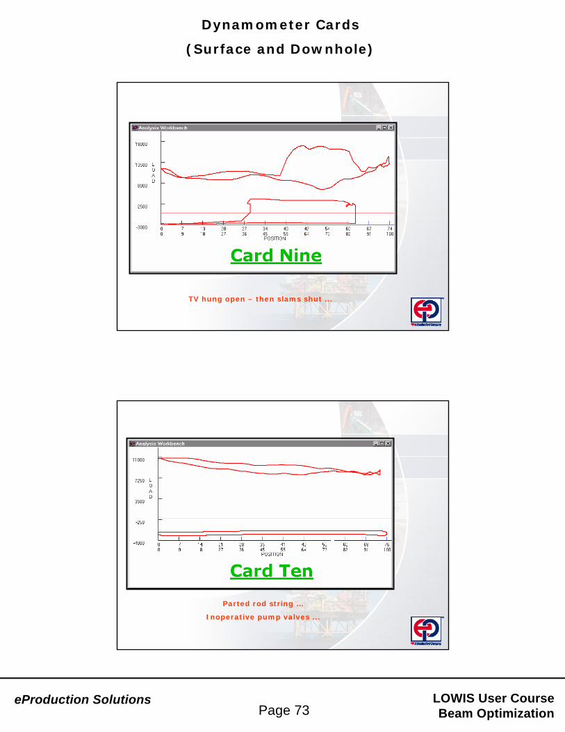
TV hung open – then slams shut ...
Parted rod string …
Inoperative pump valves ...

eProduction Solutions LOWIS User CourseBeam OptimizationPage 74
Dynamometer Cards
(Surface and Downhole)
Worn pump - upstroke leakage (TV or bbl./plunger fit) ...
SV wear, upstroke tight spot? ...

eProduction Solutions LOWIS User CourseBeam OptimizationPage 75
Dynamometer Cards
(Surface and Downhole)
Rod part ...
Stuck pump valves - trash, well not pumping ...

eProduction Solutions LOWIS User CourseBeam OptimizationPage 76
Dynamometer Cards
(Surface and Downhole)
Load cable - possible radio antenna problem ...
No tubing anchor or not enough TAC tension ...

eProduction Solutions LOWIS User CourseBeam OptimizationPage 77
Dynamometer Cards
(Surface and Downhole)
Upstroke pump wear ...
Hole in pump barrel or split pump barrel ...

eProduction Solutions LOWIS User CourseBeam OptimizationPage 78
Dynamometer Cards
(Surface and Downhole)
Upstroke pump wear ...
Timing problem – RPC SPM ...

eProduction Solutions LOWIS User CourseBeam OptimizationPage 79
Dynamometer Cards
(Surface and Downhole)
Position input problem: Proximity switch / simulated position, bad inclinometer /
potentiometer, bad real position device ...
Full pump fillage - looks good ...
eProduction Solutions LOWIS User CourseBeam OptimizationPage 80
Dynamometer Cards
(Surface and Downhole)
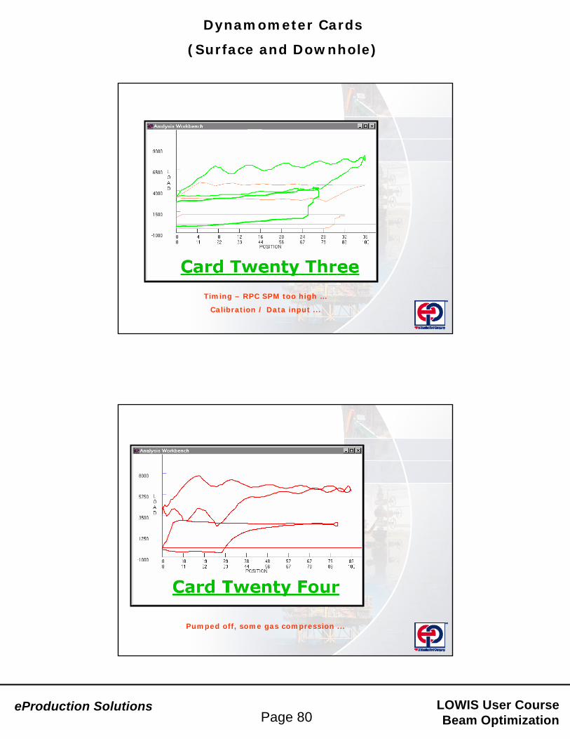
Timing – RPC SPM too high …
Calibration / Data input ...
Pumped off, some gas compression ...

eProduction Solutions LOWIS User CourseBeam OptimizationPage 81
Dynamometer Cards
(Surface and Downhole)
Sticking SV, load cable problem, load cell problem ...
Pump valves not working - trash ? ...

eProduction Solutions LOWIS User CourseBeam OptimizationPage 82
Dynamometer Cards
(Surface and Downhole)
Load cable …
Bad position input …
Tight spot in pump - sticking on downstroke ...

eProduction Solutions LOWIS User CourseBeam OptimizationPage 83
Dynamometer Cards
(Surface and Downhole)
Position input - device shaking from fluid pound or unstable foundation? ...
Bumping bottom - with reflections on upstroke ...

eProduction Solutions LOWIS User CourseBeam OptimizationPage 84
Dynamometer Cards
(Surface and Downhole)
RPC problem with “stroke” closure ? Unit rolling ?
Likely pumping unit gearbox wear ...

eProduction Solutions LOWIS User CourseBeam OptimizationPage 85
Dynamometer Cards
(Surface and Downhole)
Hitting on the upstroke …
Comments? Questions?Comments? Questions?

eProduction Solutions LOWIS User CourseBeam OptimizationPage 1
Pumping Unit Counterbalance
Pumping Unit Counterbalance
** The most overlooked component of rod pumping systems? **
Why Worry About Pumping Unit Counterbalance?
Practical field-based experience indicates that 75% of all pumping units are improperly counterbalanced. Incorrect counterbalance has two main drawbacks:
o Reduced gearbox lifeo Excessive energy usage
Remember that “balancing” a pumping unit is primarily aimed at the reduction of loading on the gearbox – and thus will not always reduce energy requirements. In some cases, energy usage may actually increase slightly. However, in cases where the unit is badly “out of balance”, energy usage will usually be reduced. One case study has shown an averageenergy use decrease of “7%-9%” per unit “balanced”. Perhaps the most important aspect of gearbox overloading caused by improper counterbalance is the effect on the life of the gearbox. A “rule of thumb” is that the life of a gearbox is reduced as the cube of the gearbox overload amount.
Example: A 320,000 in-lbs. gearbox has a calculated maximum torque of 456,000 in-lbs. (43% overload). Thus, 320000 / 456000 = (.7) cubed = 0.33 = (1/3) of the rated life of the gearbox (with ideal maintenance).
A “10%” overload reduces expected gearbox life by “25%”A “20%” overload reduces expected gearbox life by “42%”

eProduction Solutions LOWIS User CourseBeam OptimizationPage 2
Pumping Unit Counterbalance

eProduction Solutions LOWIS User CourseBeam OptimizationPage 3
Pumping Unit Counterbalance
What is “Counterbalance”?
Cranks & Counterweights (Primary / Auxiliary)

eProduction Solutions LOWIS User CourseBeam OptimizationPage 4
Pumping Unit Counterbalance
Essentially, counterbalance stores energy on the downstroke and then gives it up on the upstroke – all to reduce the required gearbox torque.
A pumping unit is said to be “weight heavy” if it has more counterbalance than is required – the weights are too big, are positioned too far out on the crank arms, or in some cases the crank arms themselves may be too large.
When referred to as “rod heavy”, a pumping unit does not have enough counterbalance – just the opposite of the “weight heavy” description.
Remember that these “out of balance” conditions or a “balanced” situation will remain constant only if the well conditions do not change because of fluid level, pump wear, downhole friction, etc. If the pumping unit is located in a waterflood or steam injection response area, changing downhole conditions mean more frequent checks and adjustments – best accomplished through the use of RPCs and central site software programs.

eProduction Solutions LOWIS User CourseBeam OptimizationPage 5
Pumping Unit Counterbalance

eProduction Solutions LOWIS User CourseBeam OptimizationPage 6
Pumping Unit Counterbalance
“Torque” is the product of a measured force (F) and the radial distance from the point of the force’s application (R) to the object rotated. (See below.)
The unit of “torque” measurement is pounds of force times inches of distance – resulting in “inch-pounds of torque”.
What is “torque” as itrelates to pumping unitgearboxes?
When considering a pumping unit gearbox, the gear reducer is subjectedto two simultaneous torques. One is the torque applied by well loads atthe polished rod transmitted through the walking beam and pittman arms.The other is the torque applied by the counterweights. (See below.)
The net torque is the algebraicsum of these two torques becausethey act in different directions. Tocomplicate matters, these appliedtorques are continually changing.

eProduction Solutions LOWIS User CourseBeam OptimizationPage 7
Pumping Unit Counterbalance
The angle of the crank is changing, thus changing the length of the moment arm of the counterbalance weights. (See below – (A) – (C).)
The angle of the walking beam at the tail bearing changes continuously(R1) and the direction that the pittman arms “pull” on the walking beam changes (R2), together causing both the lever arm length and the applied forces to change at the tail bearing. Compare “B” in the graphics above.because these forces and lever arms are changing continually, complicatedgeometrical relationships are necessary to solve them – today’s waveequation based torque analysis software programs handle this situationeasily.
Pumping unit “structural unbalance” also plays a partin determining the torque load on the gearbox.

eProduction Solutions LOWIS User CourseBeam OptimizationPage 8
Pumping Unit Counterbalance
Net Gearbox Torque (in-lbs) = TF * (W - SUB) – M SIN 0
Where –
W = Polished Rod Load (lbs.)SUB = Structural Unbalance (lbs.)TF = Torque Factor (at current crank position)M = Maximum Counterbalance (CBT, in-lbs)0 = Crank Angle (degrees)
Pumping Unit Counterbalance
“Counterbalance” can be defined as the measurement of the torque applied to a pumping unit gearbox by the unit cranks and counterweights. Basically, the term “CBE” (counterbalance effect) refers to the value of this torque as measured in the field in “pounds”. “CBT” (counterbalance torque, sometimes referred to as counterbalance “moment”) refers to this value when calculated in “in-lbs of torque”.
If a pumping unit gearbox had to supply all the force or torquenecessary to operate the entire pumping system, it would have tobe extremely large. The purpose of counterbalance (cranks and weights) is to help reduce the amount of work or torque that thegearbox has to provide to operate the system. Counterbalance helps the gearbox to handle the polished rod load on the upstroke and on the downstroke the gearbox moves the counterbalance using the rod load to help.
The Next Slide Illustrates Crank and Counterweight Counterbalance Effects

eProduction Solutions LOWIS User CourseBeam OptimizationPage 9
Pumping Unit Counterbalance

eProduction Solutions LOWIS User CourseBeam OptimizationPage 10
Pumping Unit Counterbalance

eProduction Solutions LOWIS User CourseBeam OptimizationPage 11
Pumping Unit Counterbalance

eProduction Solutions LOWIS User CourseBeam OptimizationPage 12
Pumping Unit Counterbalance
A pumping unit is said to be “balanced” when gearbox torque on the upstroke and on the downstroke is equal because the proper amount of counterbalance (cranks and counterweights) has been applied to the system.
Improperly “balanced” pumping units can and often do result in overloading the gearbox or prime mover – leading to excessive energy usage or expensive failures.
To determine if a pumping unit installation is “balanced”, use a diagnostic program that is capable of doing a torque analysis of the unit gearbox.
A less desirable method is to record the amps being using by the pumping unit on the upstroke and downstroke. Because amps are also a direct measurement of the torque requirements on the gearbox, unit “balance” or “unbalance” can be easily seen from such a measurement of amps for conventional pumping units.
Peak amp measurements are very difficult to accurately determine from “improved geometry” units (multiple peak amp readings in a single stroke).

eProduction Solutions LOWIS User CourseBeam OptimizationPage 13
Pumping Unit Counterbalance
Using data taken from an API torque analysis calculation has major advantages, especially if the information is generated by a goodcomputer analysis software program:
Counterbalance effect is easily calculated using data stored in the analysis software database - no potentially dangerous field measurements are necessary.
Counterweight placement based on calculated “optimum”counterbalance requirements eliminates "trial and error" positioning of weights when using amps as a guide. Weights are simply positioned according to analysis software calculations, greatly reducing time and cost considerations.
The risk of injury is reduced because the counterweights are “handled” only one time.
Using Measured Motor Amps vs. API Torque Analysis
Balancing beam pumped wells has traditionally been done using an amp meter or amp clamp, which requires a "trail and error" approach. This method is based on the fact that the current drawn by the electric motor is directly proportional to the work being done by the motor. The well is assumed to be balanced when the peak amps drawn on the upstroke, by the electric prime mover, is equal to the peak ampsdrawn on the downstroke. This method has several disadvantages:
It can be very time consuming (Remember, time is money) - weights may have to be adjusted several times and/or weights may have to be added or removed.
It likely will be inaccurate - the nature of using amp measurements to balance a pumping unit requires that the well be shut down for an extended period of time (likely more than once). This means a fluid level rise will occur in the casing, thus changing conditions from normal and likely causing “incorrect” amp readings. Also, improved geometry units are very difficult to balance because of multiple amp peaks during a single stroke.
It is dangerous - weights are heavy and not easy to handle, increasing the possibility of injury - especially if weights have to be removed or added to the pumping unit cranks.

eProduction Solutions LOWIS User CourseBeam OptimizationPage 14
Pumping Unit Counterbalance
When Does It Become Necessary to “Balance” a Pumping Unit?
One “rule of thumb” suggests a “10%” difference between the calculated upstroke and downstroke peak gearbox torque. This percentage should be “refined” based on torque reduction and decreased energy use for a particular operating area.
Whenever necessary to reduce unacceptable torque levels on the gearbox.
Counterbalance Measurement:
The most accurate method to measure counterbalance in the field is to use a calibrated load cell to record the polished rod load (lbs.) when a conventional pumping unit is stopped as close to “90” or “270” degrees (wellhead at the observer’s right) as possible – with the brake off. For a Mark II unit, stop the unit at the “six o’clock” position.

eProduction Solutions LOWIS User CourseBeam OptimizationPage 15
Pumping Unit Counterbalance
In most cases, however, a pumping unit will not stop in these positions and remain motionless (without using the brake) because of “unit unbalance” or other well conditions. In these situations, a chain must be used to “tie off” the polished rod to the wellhead and the unit counterbalance “propped up” or “tied off”, as appropriate, before a
measurement of counterbalance can be recorded.
Note: This method can be dangerous and should be undertaken only if absolutely required and only under the most rigorous of safe practices.
Field calculation of counterbalance is much safer, relatively simple to accomplish and provides acceptable accuracy - if the user is properly trained, and if the needed crank and weight information or counterbalance charts have been requested from the pumping unit manufacturer. There are three common scenarios that are usually encountered when “determining” counterbalance in the field.
Method One - “Formula or calculation” based counterbalance measurement:
CBT (inlbs) = CBTC (inlbs) (cranks) + CBTW (inlbs) (weights) CBTC (cranks) value is available from manufacturer information based on the individual crank identifier as observed from the cranks on each pumping unit. If this value is not provided in “inlbs.”, but in “lbs.”, use this formula to convert to “inlbs”: W (lbs.) x C.G = CBTC (inlbs.), where “W” is the weight of both cranks in pounds and “C.G” is the distance to the center of gravity of the cranks (in inches). The pumping unit manufacturer provides the “W” and “C.G” values.
CBTW (weights) = (M - X) (NW + nZ) – where …
“M” = Maximum distance from the center of the gearbox crankshaft to the center of gravity of the weight (inches)
“X” = Distance the weights are located from the long end of the cranks (inches) “N” = Number of master weights “W” = Weight of each master weight (pounds) “n” = Number of auxiliary weights “Z” = Weight of each auxiliary weight (pounds)

eProduction Solutions LOWIS User CourseBeam OptimizationPage 16
Pumping Unit Counterbalance
1. At each pumping unit, note the “ID” of each master and each auxiliary weight (if installed) and physically measure the distance from the end of the crank to the leading edge of each master weight (“X”).
2. Then, based on the “ID” of each weight – refer to the proper manufacturer’s data for the “M” distance and for the weight in pounds of each master (“W”) or auxiliary weight (“Z”).
3. Use the formula to calculate the “CBT” value of the counterweights. Add the “CBTC” (cranks) value to the “CBTW” (weights) value.
This is the “CBT” value to be entered into whatever rod pumping analysis program is being used.
Important: If more than one “size” of counterweight is used on a pumping unit, repeat the entire calculation for each different size counterweight.

eProduction Solutions LOWIS User CourseBeam OptimizationPage 17
Pumping Unit Counterbalance
Counterbalance Class Exercise 1
A Lufkin conventional pumping unit has 5456B cranks. Installed on the cranks are four # 5ARO master weights and two # 5A auxiliary weights, all measured at 6” (average distance) from the end of the cranks. From the Lufkin pumping unit catalog: “CBTC” = 70,303 inlbs., “M” = 40.1”, “W” = 913 lbs., and “Z” = 366 lbs. Calculate the “CBT” for this unit.
______________________________________________________________________________________________________________________________________________________________________________________________________________________________________________________________________________________________________________________________________________________________________________________________________

eProduction Solutions LOWIS User CourseBeam OptimizationPage 18
Pumping Unit Counterbalance
Counterbalance Class Exercise 1
A Lufkin conventional pumping unit has 5456B cranks. Located on the cranks are four # 5ARO master weights and two # 5A auxiliary weights, all measured at 6” from the end of the cranks. From the Lufkin catalog: “CBTC” = 70,303 inlbs., “M” = 40.1”, “W” = 913 lbs., and “Z” = 366 lbs. Calculate the “CBT” for this unit.
CBT (inlbs) = CBTC (inlbs) (cranks) + CBTW (inlbs) (weights)
CBTW (weights) = (M - X) (NW + nZ)CBTW = (40.1-6) * {4(913) + 2(366)}CBTW = (34.1) * {(3652) + (732)}CBTW = (34.1) * (4384)CBTW = 149,494 inlbs.
CBT = 70,303 + 149,494CBT = 219,797 inlbs.
Counterbalance Class Exercise 2
Using the same information available from exercise 1, calculate where to position the counterweights calculate (“X”) if the “optimal CBT” is 260,000 inlbs.
Was there a problem with the result?
“X” = M – {(OCBT-CBTC) / (NW + nZ)}“X” = 40.1 – {(260,000-70,303) / (4*913 + 2*366)}“X” = 40.1 – {(189,697) / (3652 + 732)} = 40.1 - {189,687 / 4384}“X” = 40.1 – 43.3“X” = - 3.2”
Yes – the negative calculation of “X” indicates that additional counterbalance needs to be added to this pumping unit in order to achieve the goal of 260,000 inlbs. of counterbalance. What is the solution?
Re-calculate “X” by adding an third auxiliary weight --
“X” = M – {(OCBT-CBTC) / (NW + nZ)}“X” = 40.1 – {(260,000-70,303) / (4*913 + 3*366)}“X” = 40.1 – {(189,697) / 3652 + 1098“X” = 40.1 – 39.9 = 0.2

eProduction Solutions LOWIS User CourseBeam OptimizationPage 19
Pumping Unit Counterbalance
Method Two – Manufacturer’s Chart-based CounterbalanceDetermination
Some pumping unit manufacturers provide counterbalance tables to enable the user to determine “CBT” (inlbs.) or “CBE” (pounds), rather than calculating CBT as explained and “exercised” in method one.
Crank and weight information still must be physically gathered from each pumping unit. Under this scenario, the cranks will have some type of “position scale” marked off on each crank.
o The counterweights will have a pointer or arrow that “points” to their position on the crank. Record the “ID” of the cranks and of each weight and weight “position” as indicated by the “pointer”. o Determine the “average” value of the position of all installed counterweights. o Then, use the appropriate manufacturer’s chart to retrieve the CBT values for the cranks and counterweights.
This is the value to be entered into an available analysis program. If the manufacturer provides only CBE (pound) charts, determine this value in the same way as described above. Analysis programs may require the conversion of CBE to CBT before calculating gearbox torque.
Once the “average” position of all installed counterweights is calculated, charts similar to those shown in the following slides can be used to determine the correct “CBT” (Maximum Moment) or “CBE” (Effective Counterbalance) value.
3.5 + 3.5 + 9.5 + 9.5 = 26 / 4 = 6.5
Average Position

eProduction Solutions LOWIS User CourseBeam OptimizationPage 20
Pumping Unit Counterbalance
CBT (in.lbs.) Counterbalance Chart
CBE (lbs.) Counterbalance Chart

eProduction Solutions LOWIS User CourseBeam OptimizationPage 21
Pumping Unit Counterbalance
Counterbalance Class Exercise 3
An American pumping unit with KA-117-53 cranks has two “RJ”master weights at position “2” and two “RJ’s” at position “10”. From the table provided on the next slide, calculate the existing “CBT”. (Note: The column labeled “Position of Counterweights” refers to the averageposition of all counterweights on the cranks.)
___________________________________________________________________________________________________________________________________________________________________________________________________________________________________________________________________________________________________________________________________________________________________________________________________________________________________________________________________________________________________________________________________

eProduction Solutions LOWIS User CourseBeam OptimizationPage 22
Pumping Unit Counterbalance
Counterbalance Class Exercise 2
An American pumping unit with KA-117-53 cranks has two “RJ” master weights at position “2” and two “RJ’s” at position “10”. From the table provided on the next slide, determine the existing “CBT”. (Note: The table column labeled “Position of Counterweights” refers to the average position of all counterweights on the cranks.)
2 + 2 + 10 + 10 = 24 / 4 = “6.0” average positionFrom the counterbalance table: “CBT” is 1,145,480 inlbs.
Note that the “CBT” and “CBE” values shown in manufacturer’s counterbalance sheets apply only to situations where there are four installed counterweights. If there are one –two – or three counterweights, these values will require adjustment based on the number of counterweights actually installed on the pumping unit.
Counterbalance Class Exercise 4
Normally, “Position of Counterweights” will very seldom be calculated as an “even” number. What changes would be required in the calculations if “average position” were calculated to be a decimal? (Ex: Not “6.0”, but “6.4”)
____________________________________________________________________________________________________________________________________________________________________________________________________________________________________________________________________________________________
From the Counterbalance Chart:
“Position 6.0” = 1,145,480 & “Position 7.0” = 1,189,4001,189,400 – 1,145,480 = 43,920 / 10 = 4,392 per decimal fraction.
Thus, an average “Position 6.4” = 1,145,480 + (4 * 4,392)“6.4” = 1,145,480 + 17,568 = 1,163,048 inlbs.

eProduction Solutions LOWIS User CourseBeam OptimizationPage 23
Pumping Unit Counterbalance
Using Counterbalance “CBE” Charts For Beam Balanced Pumping Units
Visit the wellsite and note the number and type of beam weights attached to the walking beam.
Using the correct manufacturer’s API data sheets, refer to the effective counterbalance portion of this information to determine the “CBE” value in pounds based on the number of beam weights installed.
Method Three – Host Software-based “CBT” Determination

eProduction Solutions LOWIS User CourseBeam OptimizationPage 24
Pumping Unit Counterbalance
Converting “CBE” (pounds) to “CBT” (inlbs.)
Sources of “CBE” values:
From a recent wellsite dynamometer survey measurement
From the pumping unit manufacturer’s counterbalance sheets
From “CBE” values determined by using wellsite RPC functionality
Use this formula to manually convert “CBE” to “CBT” – then enter the “CBT” value directly into an analysis program:
CBT = (CBE – SU) x TF, where -
CBT = Counterbalance torque in “inlbs.”CBE = Counterbalance effect at the polished rod in “lbs.”
SU = Structural unbalance in “lbs.” - defined as the force required at the polished rod to hold the unit walking beam in a horizontal position with the pitman arms disconnected from the crank arms. This force is “positive” when acting up on the polished rod or “negative” when exerting a downward pull. This value is included in the manufacturer’s API dimensional data sheets.
TF = Torque factor (ins.) can be defined as the number that, when multiplied by the load at the polished rod, results in the gearbox torque from that polished rod load. The pumping unit manufacturers can supply “torque factor tables” for each size unit. In addition, the number can be calculated from the unit’s geometric dimensions, but the calculations are complex and best done by a computer application.
Note: Use the “torque factor” at “90” degrees for “clockwise” unit rotation or the “torque factor” at “270” degrees for “counter-clockwise” unit rotation.

eProduction Solutions LOWIS User CourseBeam OptimizationPage 25
Pumping Unit Counterbalance
Counterbalance Class Exercise 5
Given: CBE = 17,000 lbs. TF = 68.450” SU = 480 lbs.
Calculate: CBT in “inlbs.”
CBT = (CBE – SU) x TFCBT = (17,000 – 480) * 68.450CBT = 16,520 * 68.450CBT = 1,130,794 inlbs.
This would be the value to be entered into a rod pumping analysis software program.
Field Determination of Rotaflex Counterbalance
Total CBE = Standard Minimum CBE + Auxiliary CBE
Standard Rotaflex CBE:800DX and 900 Series = 9400 lbs.1100 Series = 9800 lbs.
Auxiliary Rotaflex CBE:The auxiliary counterweights are supplied in properly
dimensioned metal blocks of varying thickness.o To calculate the weight (lbs.) of the installed auxiliary counterweights, measure each stack of auxiliary counterweights (four). Measure the height, width, and depth of each stack. (See pictures on the next slide.)
Use this formula to calculate the CBE value for eachcounterweight stack: (H” x W” x D” X 0.2833).
Add these four values together plus the “standard CBE” value for the installed Rotaflex unit size to obtain total installed CBE (lbs.).

eProduction Solutions LOWIS User CourseBeam OptimizationPage 26
Pumping Unit Counterbalance
Converting “CBE” to “CBT” in Host Analysis Software

eProduction Solutions LOWIS User CourseBeam OptimizationPage 27
Pumping Unit Counterbalance
Manual Calculations for Balancing a Pumping Unit Using Optimum Counterbalance Torque Calculations or a Counterbalance Chart
The best and most accurate method of properly balancing a pumping unit is accomplished with a diagnostic torque analysis evaluation from a “wave equation” driven analysis program. Torque analysis programs calculate the degree of “unbalance” and the increased gearbox load caused by any unit “unbalance”. Also calculated is the “optimum counterbalance torque” needed to “balance” the pumping unit, the correct weights needed, and the proper position of the counterweights.
Once “optimum counterbalance torque” value is available, the position of the weights (“X”) to achieve the “optimum counterbalance torque” can be manually calculated and thus “balance” the pumping unit.
“X” = M – {(OCBT-CBTC) / (NW + nZ)} }, where “X” is defined as the overall average distance the weights are from the end of the cranks when all weights are the same size
(Refer to the previous explanation of terms – other than “OCBT” is “optimum CBT”)
To solve for “X” when one or more of the counterweights are a different size:
“Q” = Required counterbalance torque
To move one weight:“X” = (CBTC – Q) + {M1*(W1+Z1)} + {M1*(W1+Z1)} + {M1*(W1+Z1)} ) + {M1*(W1+Z1)} (W1 + Z1)
To move two weights:“X” = (CBTC – Q) + {M1*(W1+Z1)} + {M1*(W1+Z1)} + {M1*(W1+Z1)} ) + {M1*(W1+Z1)}(W1 + Z1) + (W2 +Z2)
To move three weights:“X” = (CBTC – Q) + {M1*(W1+Z1)} + {M1*(W1+Z1)} + {M1*(W1+Z1)} ) + {M1*(W1+Z1)}(W1 + Z1) + (W2 +Z2) + (W3 + X3)
To move four weights:“X” = (CBTC – Q) + {M1*(W1+Z1)} + {M1*(W1+Z1)} + {M1*(W1+Z1)} ) + {M1*(W1+Z1)}(W1 + Z1) + (W2 +Z2) + (W3 + X3) + (W4 + Z4)
If “X” is calculated to be a negative value, add more counterweight. If “X” is calculated to be more the value of “M”, reduce the amount of counterweight.

eProduction Solutions LOWIS User CourseBeam OptimizationPage 28
Pumping Unit Counterbalance
Important:
Always move “lead” and “lag” weights to the samedistance from the end of the crank arms to prevent changing the “phase angle” of the cranks – which couldaffect gearbox torque calculation and correct counterbalance determination.
In addition, it will be necessary to use the manufacturer’s counterbalance charts when the “X” position cannot be “calculated” as indicated previously by using a formula solution.
For example:
An American pumping unit has KA-117-53 cranks with three “RJ”counterweights located at position “5” on the cranks. It has been determined that in order to “balance” the pumping unit - 1,100,000 in-lbs. of counterbalance is needed.
Where must the three counterweights be “re-positioned” to achieve this amount of counterbalance and thus “balance” the pumping unit?

eProduction Solutions LOWIS User CourseBeam OptimizationPage 29
Pumping Unit Counterbalance
From the chart above, note that the two KA-117-53 cranks and four “RJ”counterweights at position “5” have a value of 1,101,560 in-lbs. The value of the cranks alone is 551,200 in-lbs. To calculate the value of a single counterweight, subtract the value of the cranks from the total value and divide by four: (1,101,560 – 551,200) / 4 = 137,590 in-lbs. per counterweight. This means that the maximum value of the cranks and three counterweights at position “5” is: 551,200 + 3(137,590) = 963,970 in-lbs. By subtracting this number from the calculated optimum value, it can be determined how much additioncounterbalance is needed: 1,100,000 – 963,970 = 136,030 in-lbs.
Note that the counterbalance value difference between each position (“1” to “2”, “2” to “3”, “3” to “4”, etc.) is 43,920 in-lbs. To find the counterbalance value for a single counterweight, divide this number by four: 43,920 / 4 = 10,980 in-lbs.
Knowing that an additional 136,030 in-lbs. of “CBT” is needed to “balance” the unit, calculate how much “position” to add the current counterweight position of “5” for the three “RJ” counterweights: “X” = 136,030 / (3 X 10,890) = “4.1”. Therefore, “5” + “4.1” = “9.1” is the final calculated counterweight position for the three “RJ”counterweights.

eProduction Solutions LOWIS User CourseBeam OptimizationPage 30
Pumping Unit Counterbalance
API Torque Analysis Counterbalance Adjustment Benefits
Studies have shown:
☺ Peak gearbox torque is reduced an average of 17% per well
☺ Power cost is reduced an average of 8% per year
COUNTERBALANCE IS IMPORTANT !!!