Dynamics of solvency riskin life insurance liabilities∗

M.C. Christiansen† and M.A. Fahrenwaldt‡

We describe the time dynamics of the solvency level of life insurance contractsby representing the solvency level and the underlying risk sources as the solutionof a forward-backward system. This leads to an additive decomposition ofthe total solvency level with respect to time and different risk sources. Thedecomposition turns out to be an intuitive tool to study risk sensitivities. Westudy the forward-backward system and discuss two methods to obtain explicitrepresentations: via linear partial differential equations and via a Monte Carlomethod based on Malliavin calculus.

Keywords: solvency level; life insurance risk management; backward stochastic differen-tial equation; Malliavin calculus.

1. Introduction

The solvency level of insurance contracts has always been a key quantity in actuarial riskmanagement. The so-called top-down method (cf. Buhlmann (1985)) derives managementdecisions on premiums, reserves, surplus redistribution, etc. from a stability goal determinedin advance. The European solvency regime ’Solvency II’ (cf. CEIOPS (2009)) imposesa minimum 99.5% solvency probability over one year as stability criterion for insurancecompanies.

For insurers it is vital to understand and control their solvency level. While the regulatoris interested in a portfolio perspective, we focus on individual contracts, which is relevant in

∗This is an Accepted Manuscript of an article published by Taylor & Fran-cis Group in Scandinavian Actuarial Journal on 20/03/2015, available online:http://www.tandfonline.com/10.1080/03461238.2015.1020856.

†Maxwell Institute for Mathematical Sciences, Edinburgh, and Department of Actuarial Math-ematics and Statistics, Heriot-Watt University, Edinburgh, EH14 4AS, United KingdomM.C.Christiansen@hw.ac.uk

‡Institut fur Mathematische Stochastik, Leibniz Universitat Hannover, Welfengarten 1, 30167Hannover, Germany and EBZ Business School, Springorumllee 20, 44795 Bochum, Germanyfahrenw@stochastik.uni-hannover.de

1

actuarial risk management for contract design, redistribution of surplus, contract valuation,etc. Since unsystematic mortality risks are largely diversifiable by increasing the size of theinsurance portfolio, our attention is only on systematic mortality risk and financial risk.

Modern solvency risk management is a continuous effort based on monitoring of risksand reacting timely when necessary. This motivates to take a dynamic perspective withina time-continuous framework. To give an informal summary of the results, denote by thestochastic process N the net value of the contract, which we define as the difference ofretrospective reserve and prospective liabilities. Each depends on underlying demographicand economic variables (e.g. interest rate, mortality rate, etc.) modeled as vector-valueddiffusion process X. The latter process is driven by a multidimensional Brownian motionW with associated filtration (Ft)t representing the information available up to time t. Wesay that the insurance contract is solvent at time t if Nt ≥ 0. We are then able to expressthe change in the solvency probability at expiry T as

P(NT ≥ 0|Ft)−P(NT ≥ 0|F0) =

∫ t

0

U>r dMXr =

∫ t

0

Z>r dWr. (1.1)

Here, MXr is the martingale part of X according to Doob’s decomposition, representing the

random fluctuations in the underlying demographic and economic variables. The adaptedprocess U is vector-valued and represents the contributions of the different demographic andeconomic variables at each time r to the overall solvency risk. In an alternative viewpointtaken here, an adapted process Z describes the effect that the Brownian driver W has onthe solvency level.

Technically, we model the dynamics of P(Nt ≥ 0|Ft) using a forward-backward system,i.e. a combination of a forward and a backward stochastic differential equation. Besidesthis conceptual investigation we also discuss the implementation of such a scheme, whichis a nontrivial task here. First of all, the probability P(Nt ≥ 0|Ft) can be expressed as adeterministic function of Xt and the present value of the past surplus. We characterize thisfunction using a linear partial differential equation. Moreover, we sketch two approachesto numerically obtain the process Z. The first ansatz links the forward-backward systemto a linear partial differential equation as in the classical Feynman-Kac analysis albeit withtechnical difficulties. As an alternative we also present a Monte-Carlo simulation approachwith the help of Malliavin calculus that applies in more general situations at the expenseof higher technical demands.

As the actuary typically works in two pictures, namely the partial differential equationsand the stochastic analysis picture, we develop these perspectives in parallel and discusstheir relationship. We employ only basic theory of backward stochastic differential equa-tions and Malliavin calculus. However, the focus of this paper is an actuarial applicationof these techniques and not an exercise in abstract stochastic analysis.

Once the solvency probabilities P(Nt ≥ 0|Ft) are available, various further (for examplequantile-based) risk measures are within reach. Also, the formulation with the forward-backward system lends itself easily to important applications and generalizations that arebeyond the scope of the current paper. First, the class of g-expectations (cf. Peng (1997),Rosazza Gianin (2006) and references therein) leading to dynamic risk measures appliedto the solvency probability is naturally phrased in terms of our forward-backward system.

2

Second, highly topical in insurance practice is the solvency-optimal control of actuarial man-agement parameters. Our forward-backward system provides the groundwork for stochasticcontrol with solvency level objectives.

While our approach to study the dynamics of the solvency level seems to be new, thereis a rich literature on the dynamics of the expectation of life insurance liabilities. Twostrands can be distinguished by the measure they use to value liabilities. Assuming thatthe underlying demographic and economic risks are traded on a financial market, the ex-pectation with respect to a (risk-neutral) market measure describes the market value of theinsurance liabilities. For more details and further references we recommend the compre-hensive presentations in Møller & Steffensen (2007) and Delong (2013). Schilling, Bauer,Christiansen & Kling (2015) study the dynamics of the expectation with respect to the real-world measure, aiming to decompose the total randomness in the liabilities with respectto different demographic and economic variables. We follow their concept of additive riskdecomposition with respect to time and different risk sources, yet unlike them, we employFBSDE techniques and focus on non-Lipschitz terminal conditions.

The use of backward stochastic differential equations in finance is well-established, cf.El Karoui, Peng & Quenez (1997) for an early survey. Their use in actuarial mathematicsappears to be mainly in defining replicating strategies for liabilities as in Delong (2010)and finding optimal hedging strategies for them, cf. Delong (2012). Many models involvejump processes, so they are technically considerably advanced.

This paper is organised as follows. The following section contains the basic definitions ofthe solvency probability and gives actuarial examples. Section 3 describes the evolution ofthe reserves and solvency probabilities using stochastic analysis. The simulation of theseprocesses is discussed in Section 4. The final section contains a worked example based onOrnstein-Uhlenbeck processes to which the numerical methods are applied.

2. Actuarial motivation: prospective liabilities,retrospective reserve and net values in life insurance

This section motivates the definition of the solvency position of individual life insurancecontracts. Precise technical assumptions on coefficient functions are made in the latersections.

The prospective liabilities of a life insurance contract at time t can usually be describedby

V +t = f(XT ) e−

∫ Tt k(τ,Xτ ) dτ +

∫ T

t

g(s,Xs) e−∫ st k(τ,Xτ ) dτ ds, (2.1)

where T > 0 is a finite time horizon and the functions f, g, k are suitably regular. Theprocess X describes the actuarial assumptions (demographic and economic variables) andshall be an n-dimensional diffusion process of the form

dXt = µ(t,Xt) dt+ σ(t,Xt) dWt, t ∈ (0, T ]

X0 = x0

(2.2)

3

with x0 ∈ Rn. The factor exp−∫ Ttk(τ,Xτ ) dτ describes financial discounting and bio-

metric discounting, i.e. survival or decrement rates. The functions f and g correspond toa terminal payment at T and continuous payments in (0, T ), respectively. The stochasticprocess V +

t is the pathwise solution of the stochastic differential equationdV +

t =(k(t,Xt)V

+t − g(t,Xt)

)dt, t ∈ [0, T )

V +T = f(XT ).

(2.3)

As V +t depends on the future of the process X, it is not adapted to the natural filtration

generated by X.

Example 2.1 (Prospective reserve of a life insurance). Suppose that Xt =(X

(1)t , X

(2)t

)>describes an interest intensity X

(1)t = φ(t) and a mortality intensity X

(2)t = µ(a + t) of a

policyholder with initial age a at contract time t = 0. The randomness of Xt expressesthe uncertainty on future returns on investments and future systematic changes of survivalrates. Denote by T the termination time of a life insurance contract with annuity paymentrate b(t), death benefit c(t) in case of death at time t, and a lump sum survival benefit ofBT at time T . Letting

k(t, x1, x2) = x1 + x2,

g(t, x1, x2) = b(t) + c(t)x2,

f(x1, x2) = BT ,

the functional V +t has the form

V +t = BT e

−∫ Tt (φ(τ)+µ(a+τ))dτ +

∫ T

t

(b(s) + c(s)µ(a+ s)) e−∫ st (φ(τ)+µ(a+τ))dτ ds.

In classical life insurance, where φ and µ are modelled deterministically, we call V +t the

prospective reserve at time t in state alive. When modelling φ and µ stochastically, theterm ’prospective reserve’ might be misleading, since V +

t is not Ft-adapted, so that thisvalue is unknown and cannot be reserved at time t.

Solving the stochastic differential equation (2.3) with initial value v0 instead of terminalvalue f(XT ),

dV −t =(k(t,Xt)V

−t − g(t,Xt)

)dt, t ∈ (0, T ]

V −0 = v0,(2.4)

we obtain a stochastic process V −t that is explicitly given as

V −t = v0 e∫ t0 k(τ,Xτ ) dτ −

∫ t

0

g(s,Xs) e∫ ts k(τ,Xτ ) dτ ds. (2.5)

In contrast to V + the stochastic process V − is adapted to the natural filtration generatedby X.

4

Example 2.2 (Retrospective reserve of a life insurance). Let v0 = −B0, where B0 is a lumpsum premium at time t = 0. We put a negative sign to the premium since the paymentgoes in the other direction than the annuity payments, the death benefit and the survivalbenefit. In the setting of Example 2.1, the process V −t has the form

V −t = −B0 e∫ t0 (φ(τ)+µ(a+τ))dτ −

∫ t

0

(b(s) + c(s)µ(a+ s)) e∫ ts (φ(τ)+µ(a+τ))dτ ds

and represents the retrospective reserve of the contract at time t in state alive. The ret-rospective reserve corresponds to the present value of assets that belong to the insurancecontract.

For further examples from finance and insurance see Sondermann (2006) and Møller &Steffensen (2007).

Since the prospective process V +t and the retrospective process V −t can be interpreted as

the prospective liabilities at time t and the accrued assets at time t, we make the

Definition 2.3. Let the processes V + and V − be solutions of (2.2) and (2.4), respectively.We call

Nt := V −t − V +t , t ∈ [0, T ]

the net value at time t of the life insurance contract.

Note that the net valueNt differs from the concept of the ’net present value’ in accounting.The difference is that Nt depends on random future events, so that Nt is not observable attime t. In contrast, in accounting the prospective liabilities are defined as mark-to-modelor mark-to-market future payment obligations, so that the accounting value process wouldbe adapted.

The next lemma shows that the sign of Nt does not depend on time t.

Lemma 2.4. Nt = N0 e∫ t0 k(τ,Xτ ) dτ for all t ∈ [0, T ]. The random variable N0 depends on

the path of X from t = 0 until t = T . It is therefore not adapted to the natural filtrationgenerated by X.

Proof. Follows from (2.1) and (2.5).

A key question in practice is whether Nt is positive or negative, indicating if the lifeinsurance policy creates a gain or a loss. This will be the focus of our paper.

Example 2.5 (Solvency level). In insurance regulation according to Solvency II, the prob-ability over a one year period that the assets of an insurer are greater than or at least equalto the insurers liabilities shall be at least 99.5%. In banking regulation according to BaselII/III similar rules apply. By setting T = 1 and interpreting v0 as the insurers equity attime zero and f(X1) as the (market-consistent) value at time 1 of the insurers liabilities onthe timeline [1,∞), the solvency rule can be written as

P(N1 ≥ 0

∣∣X0

)≥ 0.995. (2.6)

In order to check that condition, we need to find a way to calculate the conditional proba-bility in (2.6).

5

Note that Solvency II imposes (2.6) on the portfolio level, while we focus on individualcontracts. The individual perspective, however, is significant in actuarial risk managementas it helps to understand how each contract contributes to the overall solvency situation.Insurance companies have only limited tools for their capital management so that a risk-based strategic management needs the individual perspective to direct its underwritingactivities to business that matches the available capital.

The focus of this paper is to develop and discuss the representation (1.1). Due to theMarkovian nature of the processes involved, we have

P(NT ≥ 0

∣∣Ft) = P(NT ≥ 0

∣∣Xt, V−t

).

We note an immediate corollary of the latter equation.

Lemma 2.6. The distribution function of V +t conditional on Xt is given by

P(V +t ≤ v

∣∣Xt = x)

= P(NT ≥ 0

∣∣Xt = x, V −t = v)

for all t ∈ [0, T ], x ∈ R.

Proof. The assertion follows from the equality of the events NT ≥ 0 = Nt ≥ 0 accord-ing to Lemma 2.4, from the equality of the events Nt ≥ 0 = V +

t ≤ v conditional onV −t = v, and from the Markov property of the process X.

Lemma 2.6 adds another motivation for calculating (1.1): the conditional distributionfunction of V +

t is of key importance in accounting when the prospective liabilities V +t are

to be evaluated by some (for example quantile-based) risk measure. Our results for (1.1)will also allow to calculate the conditional distribution function of V +

t .

3. The evolution of retrospective and prospectiveprocesses and the net value

The aim of this section is to formulate the behaviour of the solvency probability P(NT ≥0|Ft) as the solution of a forward-backward system. We proceed in steps and first givea forward-backward system for the dynamics of the prospective liabilities, a stochasticdifferential equation (SDE) for the pair (Xt, V

−t ), and then construct a backward stochastic

differential equation (BSDE) with terminal condition 1(NT ≥ 0) to study the dynamics andregularity of the solvency process. We then obtain the desired probability P(NT ≥ 0|Ft)as E(1(NT ≥ 0)|Ft).

We make the following overarching assumptions valid throughout the paper.Let (Ω,F ,P) be a probability space on which there is an n-dimensional Brownian motion

denoted by Wt = (W(1)t , . . . ,W

(n)t )> with corresponding filtration Ft.

Assumption 3.1. Suppose that there are Borel measurable functions µ : [0, T ]×Rn → Rn

and σ : [0, T ] × Rn → Rn×n with σ matrix-valued. Assume that µ and σ are globally

Lipschitz and at most of linear growth at infinity:

||µ(s, x)− µ(s, y)||+ ||σ(s, x)− σ(s, y)|| ≤ K||x− y||,||µ(s, x)||2 + ||σ(s, x)||2 ≤ K2

(1 + ||x||2

),

6

for every s ∈ [0, T ] and x, y ∈ Rn and some constant K > 0. Here, || · || denotes theEuclidean norm.

To describe the evolution of the prospective liabilities and the retrospective reserve weneed further assumptions.

Assumption 3.2. Let k and g be Borel measurable functions [0, T ]× Rn → R such that

||k(s, x)− k(s, y)||+ ||g(s, x)− g(s, y)|| ≤ K||x− y||,||g(s, x)|| ≤ K(1 + ||x||),||k(s, x)|| ≤ K

for some constant K, all s ∈ [0, T ] and x, y ∈ Rn.

Remark 3.3. Note that the function k in Example 2.1 is not bounded. Restricting itto the class of bounded functions means that we impose lower and upper bounds for theinterest rate and the mortality rate. However, the bounds may be chosen arbitrarily large,so this is an insignificant restriction from the perspective of insurance practice.

3.1. Backward stochastic differential equations

We briefly recall the notion of a BSDE with precise technical details to follow below. BS-DEs were introduced in the linear case in Bismut (1973) and the theory has found applica-tions in stochastic optimal control, PDEs (Pardoux & Peng (1992)), financial mathematics(El Karoui et al. (1997)) and nonlinear expectations (Peng (1997)). We refer the reader toPardoux & Rascanu (2014) for detailed references.

Loosely speaking, a solution of a BSDE is a pair of adapted stochastic processes (Y, Z)with the terminal condition YT = ξ such that

−dYs = F (s, Ys, Zs) ds− Z>s dWs

YT = ξ

or equivalently Ys = ξ+∫ TsF (r, Yr, Zr) dr−

∫ TsZ>r dWr whereW denotes a multidimensional

Brownian motion. The function F is called the driver of the BSDE. The process Z is alsomultidimensional and is commonly known as the control process.

To illustrate the application in mathematical finance for example in the pricing of deriva-tives: the process Ys reflects the value of the contingent claim at time s and Zs can be viewedas the portfolio process of the hedging strategy, cf. El Karoui et al. (1997). For insuranceapplications—which appear to be much rarer—we refer the reader to Delong (2013) fordetailed examples.

We specialize to the case where the driver is zero and the terminal condition is a functionof X. The BSDE is called Markovian in this case. It is expressed as a forward-backwardsystem of an SDE and a BSDE and naturally leads to a PDE.

By the solution of a BSDE we mean a pair of processes (Ys, Zs) such that Ys|s ∈ [0, T ]is a continuous R-valued adapted process and Zs|s ∈ [0, T ] is an Rn-valued predictable

process satisfying∫ T

0||Zs||2ds <∞, P-a.s.

7

3.2. A forward-backward system for the prospective liabilities

For completeness and to indicate the role of the usual Thiele equation for the prospectiveliabilities, we describe the evolution of the liabilities by a forward-backward system. Thisalso yields a novel perspective on the dynamics of the liabilities not yet discussed in theliterature.

Recall that the prospective liabilities were given by a process

V +(t,x)s = f

(X

(t,x)T

)e−∫ Ts k

(τ,X

(t,x)τ

)dτ

+

∫ T

s

g(r,X(t,x)

r

)e−∫ rs k(τ,X

(t,x)τ

)dτdr. (3.1)

By the superscript (t, x) we mean that the process X starts at x at time t. Intuitively, theprospective liabilities should be formulated as a BSDE with suitable terminal condition atleast modulo a control process. The BSDE for V

+(t,x)s is given by (cf. (2.3))

Ys = f(XT ) +

∫ T

s

(−k(r,Xr)Yr + g(r,Xr)) dr −∫ T

s

Z>r dWr. (3.2)

The combination of (2.2) and (3.2) is commonly known as an (uncoupled) forward-backward system, cf. El Karoui (1997), Pontier (1997), Ma & Yong (1999).

We seek a unique solution of the BSDE (3.2) in a suitable function space. DefineH

2T (Rd) to be the space of all predicable processes Ψ : Ω × [0, T ] → R

d such that

E

(∫ T0||Ψt||2dt <∞

). We call these processes square-integrable.

Proposition 3.4. Suppose that Assumptions 3.1 and 3.2 hold. Then the forward-backwardsystem

dXs = µ(s,Xs)ds+ σ(s,Xs)dWs, Xt = x, t ≤ s ≤ T−dYs = (−k(s,Xs)Ys + g(s,Xs)) ds− Z>s dWs, YT = f(XT ), t ≤ s ≤ T

has a unique square-integrable solution(X

(t,x)s , Y

(t,x)s , Z

(t,x)s

). Also, the prospective liabilities

are given by

V +(t,x)s = Y (t,x)

s +

∫ T

s

e−∫ rs k(τ,X

(t,x)τ )dτZ(t,x)

r

>dWr. (3.3)

Proof. Existence and uniqueness follows from Pardoux & Peng (1990). The second assertionconcerning the form of the solution is a consequence of the linearity of the BSDE, cf. Remark5.38 of Pardoux & Rascanu (2014).

A consequence is the

Corollary 3.5. The process Y(t,x)t is deterministic and can be represented by a function

u(t, x) := Y(t,x)t = E

(Y

(t,x)t

)= E

(V

+(t,x)t

).

Proof. The fact that Y(t,x)t is deterministic follows from the iterative construction of the

BSDE solution, cf. Pardoux & Peng (1992) so that Y(t,x)t = E

(Y

(t,x)t

). Since the expecta-

tion of the Ito integral in (3.3) is zero, the claim u(t, x) = E

(V

+(t,x)t

)follows.

8

The control process Z is obtained by the martingale representation theorem as the uniquesquare-integrable process such that

f(X

(x,t)T

)= E

(f(X

(x,t)T

))+

∫ T

t

Z(t,x)s

>dWs.

This is a mere existence result that does not yield exact information on Z. However, dueto the Markovian nature of our setting we can express (Y, Z) by measurable functions of(X, V −). In certain circumstances which we describe later these functions can be obtainedas a PDE solution and its gradient, respectively.

Proposition 3.6 (El Karoui et al. (1997), Theorem 4.1). There exist two measurabledeterministic functions u : [0, T ]×Rn → R and d : [0, T ]×Rn → R

n+1 such that

Y (t,x)s = u

(s,X(t,x)

s

),

Z(t,x)s = σ

(s,X(t,x)

s

)>d(s,X(t,x)

s

).

It is profitable to interpret (3.3) actuarially. Applying Proposition 3.6 and assuming thatthe probability measure corresponds to a (risk-neutral) market measure, one can view (3.3)as

V +(t,x)s︸ ︷︷ ︸

prospective liabilities

= Y (t,x)s︸ ︷︷ ︸

present value of theprospective liabilities

+

∫ T

s

e−∫ rs k(τ,X

(t,x)τ

)dτd(r,X(t,x)

r

)>︸ ︷︷ ︸hedging strategy

σ(r,X(t,x)

r

)dWr︸ ︷︷ ︸

market price changesin the underlyings

.

Under the real world probability measure, one can view (3.3) as

V +(t,x)s︸ ︷︷ ︸

prospective liabilities

= Y (t,x)s︸ ︷︷ ︸

best estimate for theprospective liabilities

+

∫ T

s

e−∫ rs k(τ,X

(t,x)τ

)dτ︸ ︷︷ ︸

discounting factor

d(r,X(t,x)

r

)>︸ ︷︷ ︸sensitivity factor

σ(r,X(t,x)

r

)dWr︸ ︷︷ ︸

random fluctuationsin the underlyings

.

It makes indeed sense to interpret Y(t,x)s as a best estimate for the prospective liabilities

given all the information available at time s, since Y(t,x)s = E

(V

+(t,x)s

∣∣∣Fs). The Ito integral

describes the random fluctuations around the best estimate and consists of the followingparts:

• A discounting factor e−∫ rs k(τ,X

(t,x)τ

)dτ

. In Example 2.1 this factor includes both, afinancial discounting and a biometrical discounting (the survival rate).

• A sensitivity factor d(s,X

(t,x)s

)that describes the monetary effect that the random

fluctuations of X have on the prospective liabilities.

• The martingale part σ(s,X

(t,x)s

)dWr of the integrator dXr, describing the random

fluctuations of the underlying process X.

9

Example 3.7. Following the ideas in the previous remark, for Example 2.1 we obtain

V +(t,x)s = E

(V +(t,x)s

∣∣Fs)+

∫ T

s

e−∫ rs φ(τ)dτ︸ ︷︷ ︸

financial discounting

e−∫ rs µ(a+τ)dτ︸ ︷︷ ︸

survival rate

d(r,X(t,x)

r

)>︸ ︷︷ ︸sensitivity factor

d

(Mµ(a+ r)

Mφ(r)

)︸ ︷︷ ︸

random fluctuationsin the underlyings

,

(3.4)

where Mµ(a+ r) and Mφ(r) denote the martingale parts of the diffusion processes µ(a+ r)and φ(r).

The above risk decomposition under the real world probability measure equals the lim-iting case of the risk decomposition presented by Schilling et al. (2015) as the portfoliosize goes to infinity. Schilling et al. (2015) define the risk decomposition with the help ofthe martingale representation theorem and calculate more explicit formulas by employingMalliavin calculus and Ito’s formula, assuming regularity of the diffusion matrix and differ-entiability of the terminal condition. Our approach avoids the latter two conditions, whichwill be essential for decomposing the solvency probability later on. Note that Schillinget al. (2015) also offer a comprehensive discussion on why the risk decomposition conceptof above is extremely useful in actuarial risk management. Formula (3.4) has also simi-larities with the classical surplus decomposition formula: Let (φ, µ) be a best estimate for

(φ, µ) and write V+

s for the prospective reserve calculated on the basis of (φ, µ). Accordingto Norberg (2001) the surplus decomposition formula yields here

V +s = V

+

s +

∫ T

s

e−∫ rs φ(τ)dτ︸ ︷︷ ︸

financial discounting

e−∫ rs µ(a+τ)dτ︸ ︷︷ ︸

survival rate

(c(r)− V +

r

−V +

r

)>︸ ︷︷ ︸

sensitivity factor

(µ(a+ r)− µ(a+ r)

φ(r)− φ(r)

)dr︸ ︷︷ ︸

deviationsin the underlyings

.

In (3.4) the integrator describes the instantaneous improvements and deteriorations ofµ and φ at time r, whereas in the surplus decomposition formula the integrator (µ(a +r) − µ(a + r), φ(r) − φ(r))>dr includes all improvements and deteriorations on the wholeinterval [0, r]. So formula (3.4) better allows to separate the risk contributions of differenttime intervals.

A similar multiplicative decomposition of the reserves into risk types is obtained inFahrenwaldt (2015) using semigroup theory and representing different risks by linear oper-ators.

To study the regularity of u and d, we can link the evolution of the prospective liabilitiesto the well-known Thiele differential equation (cf. Norberg (1991), Steffensen (2000), Møller& Steffensen (2007)). In our case it is given by

∂tu(t, x) +Au(t, x) + (−k(t, x)u(t, x) + g(t, x)) = 0

u(T, x) = f(x),(3.5)

where the partial differential operator A is defined as

A = 12

n∑i,j=1

[σσ>

]ij

(t, x)∂xi∂xj +n∑i=1

µi(t, x)∂xi .

10

Here, ∂t = ∂∂t

and ∂xi = ∂∂xi

for i = 1, . . . , n.To state this link we briefly recall the notion of a viscosity solution, cf. Crandall, Ishii

& Lions (1992) or Fleming & Soner (2006). Consider the general terminal value problem−∂tu(t, x) + F (t, x,Dxu(t, x), D2

xu(t, x)) = 0, (t, x) ∈ [0, T )×Rd

u(T, x) = ψ(x), x ∈ Rd.(3.6)

for some bounded function ψ. Here, Dxu stands for the collection of first derivatives ∂xiuand D2

x for the collection of second-order derivatives ∂xi∂xju.

Definition 3.8. Let F be a continuous function. We say that u is a

(i) viscosity subsolution of (3.6) if for each w ∈ C∞([0, T )×Rn),

−∂tw(t0, x0) + F(t0, x0, Dxw(t0, x0), D2

xw(t0, x0))≤ 0

at every (t0, x0) ∈ [0, T )×Rn that is a strict maximizer of u−w on [0, T ]×Rn withu(t0, x0) = w(t0, x0);

(ii) viscosity supersolution of (3.6) if for each w ∈ C∞([0, T )×Rn),

−∂tw(t0, x0) + F(t0, x0, Dxw(t0, x0), D2

xw(t0, x0))≥ 0

at every (t0, x0) ∈ [0, T )×Rn that is a strict minimizer of u− w on [0, T ]×Rn withu(t0, x0) = w(t0, x0);

(iii) viscosity solution if it is both a viscosity subsolution and a viscosity supersolution.

Standard BSDE theory then yields the desired link between BSDE and PDE.

Proposition 3.9. Under the Assumptions 3.1 and 3.2, the following holds.

(i) The function u is continuous in (t, x) ∈ [0, T ] × Rn and it is the unique viscositysolution of the partial differential equation (3.5) which grows at most polynomially atinfinity.

(ii) If the coefficients σ, µ, k, g and the terminal condition f are three times continuouslydifferentiable with bounded derivatives, then u is a classical solution of (3.5) andbelongs to C1,2([0, T ]×Rn).

(iii) In the latter case, the solution of the BSDE (3.2) is given by Y(t,x)s = u

(s,X

(t,x)s

)and Z

(t,x)s = σ

(s,X

(t,x)s

)>∇u(s,X

(t,x)s

)for any t ≤ s ≤ T where ∇ = (∂x1 , . . . , ∂xn)

is the gradient operator.

Proof. The assertion on the viscosity solution is Theorem 5.37 of Pardoux & Rascanu(2014). The second assertion on the classical solution is Theorem 3.2 of Pardoux & Peng(1992). The third assertion is Corollary 4.1 of (El Karoui et al. 1997).

11

Remark 3.10. Vice versa, if u ∈ C1,2([0, T ] × Rn) is a classical solution of (3.5) then

Ito’s Lemma shows that Y(t,x)s = u

(s,X

(t,x)s

)and Z

(t,x)s = σ

(s,X

(t,x)s

)>∇u(s,X

(t,x)s

),

cf. Proposition 4.3 of El Karoui et al. (1997). At inception of the contract we have

Y(t,x)t = u(t, x) and Z

(t,x)t = σ(t, x)>∇u(t, x).

Indeed, we recover the usual Feynman-Kac theorem in the form

V+(t,x)t = E

[f(X

(t,x)T

)e−∫ Tt k

(τ,X

(t,x)τ

)dτ

+

∫ T

t

g(r,X(t,x)

r

)e−∫ Tt k

(τ,X

(t,x)τ

)dτ

dr

]at the inception of the contract.

The solutions of the Thiele equation (3.5) can now be further analyzed using functionalanalytic tools, cf. Christiansen (2008) or Fahrenwaldt (2015).

3.3. An SDE for the economic variables and the retrospective reserve

The evolution of the retrospective reserve can be represented by a forward SDE. Thisis the forward component of the forward-backward system constructed in the subsequentsubsection.

Proposition 3.11. Suppose that Assumptions 3.1 and 3.2 hold. Then for every choice ofinitial condition (t, x, v) ∈ [0, T ]×Rn ×R the stochastic differential equation(

Xs

V −s

)=

(xv

)+

∫ s

t

(µ (τ,Xτ )

k (τ,Xτ )V−τ − g (τ,Xτ )

)dτ +

∫ s

t

(σ (τ,Xτ )

0

)dWτ , (3.7)

where 0 ≤ t ≤ s ≤ T , has a unique strong solution(X

(t,x)s , V

−(t,x,v)s

)>which is square

integrable.

Proof. This is Theorem 2.9 in Chapter 5 of Karatzas & Shreve (1991).

In the more compact differential notation, we can express the SDE (3.7) asd(Xs, V

−s

)>= µ(s,Xs, V

−s )ds+ σ(s,Xs)dWs, 0 ≤ t ≤ s ≤ T

(Xt, V−t )> = (x, v)>

with

µ(s, x, v) =

(µ(s, x)

k(s, x)v − g(s, x)

)∈ Rn+1,

σ(s, x) =

(σ(s, x)

0

)∈ R(n+1)×n.

(3.8)

We will work with these matrix valued functions from now on.

12

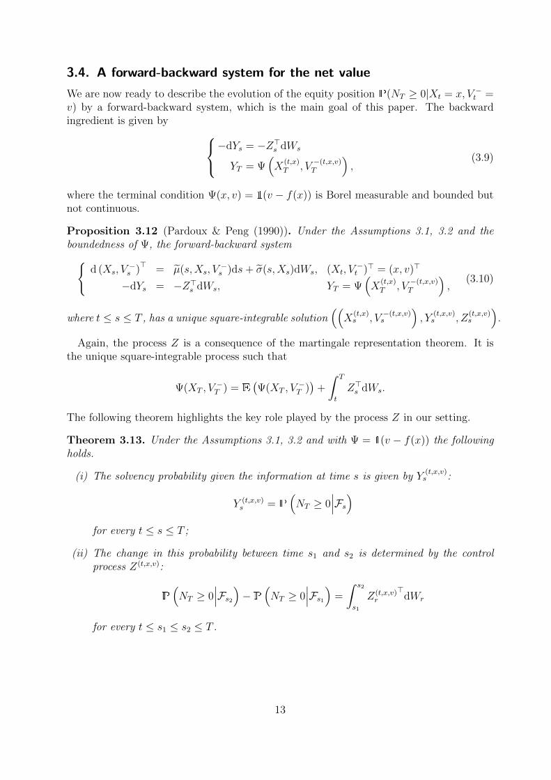
3.4. A forward-backward system for the net value

We are now ready to describe the evolution of the equity position P(NT ≥ 0|Xt = x, V −t =v) by a forward-backward system, which is the main goal of this paper. The backwardingredient is given by −dYs = −Z>s dWs

YT = Ψ(X

(t,x)T , V

−(t,x,v)T

),

(3.9)

where the terminal condition Ψ(x, v) = 1(v − f(x)) is Borel measurable and bounded butnot continuous.

Proposition 3.12 (Pardoux & Peng (1990)). Under the Assumptions 3.1, 3.2 and theboundedness of Ψ, the forward-backward system

d (Xs, V−s )>

= µ(s,Xs, V−s )ds+ σ(s,Xs)dWs, (Xt, V

−t )> = (x, v)>

−dYs = −Z>s dWs, YT = Ψ(X

(t,x)T , V

−(t,x,v)T

),

(3.10)

where t ≤ s ≤ T , has a unique square-integrable solution((X

(t,x)s , V

−(t,x,v)s

), Y

(t,x,v)s , Z

(t,x,v)s

).

Again, the process Z is a consequence of the martingale representation theorem. It isthe unique square-integrable process such that

Ψ(XT , V−T ) = E

(Ψ(XT , V

−T ))

+

∫ T

t

Z>s dWs.

The following theorem highlights the key role played by the process Z in our setting.

Theorem 3.13. Under the Assumptions 3.1, 3.2 and with Ψ = 1(v − f(x)) the followingholds.

(i) The solvency probability given the information at time s is given by Y(t,x,v)s :

Y (t,x,v)s = P

(NT ≥ 0

∣∣∣Fs)for every t ≤ s ≤ T ;

(ii) The change in this probability between time s1 and s2 is determined by the controlprocess Z(t,x,v):

P

(NT ≥ 0

∣∣∣Fs2)−P(NT ≥ 0∣∣∣Fs1) =

∫ s2

s1

Z(t,x,v)r

>dWr

for every t ≤ s1 ≤ s2 ≤ T .

13

Proof. (i) Note that due to the driver of the BSDE being zero we can explicitly give the

solution Y(t,x,v)s as

Y (t,x,v)s = E(Ψ(X

(t,x)T , V

−(t,x,v)T |Fs), (3.11)

which we interpret as P(NT ≥ 0|Fs) as V−(t,x,v)T − f(X

(t,x)T ) = V −T − V

+T = NT .

(ii) We find from the integral version of (3.9) that

Y (t,x,v)s = Ψ(X

(t,x)T , V

−(t,x,v)T )−

∫ T

s

Z(t,x,v)r

>dWr

for every t ≤ s ≤ T . So using (3.11) one has

Y (t,x,v)s2

− Y (t,x,v)s1

=

(Ψ(X

(t,x)T , V

−(t,x,v)T )−

∫ T

s2

Z(t,x,v)r

>dWr

)−(

Ψ(X(t,x)T , V

−(t,x,v)T )−

∫ T

s1

Z(t,x,v)r

>dWr

)=

∫ s2

s1

Z(t,x,v)r

>dWr

which is precisely the assertion.

Analogously to Corollary 3.5, according to Proposition 3.6 there exists a deterministicfunction u such that we can rephrase Theorem 3.13 as follows.

Corollary 3.14. (i) There exists a measurable deterministic function u : [0, T ] ×Rn ×R → R such that the solvency probability given the information at time s has therepresentation

P

(NT ≥ 0

∣∣∣Fs) = u(s,X(t,x)

s , V −(t,x,v)s

)for every t ≤ s ≤ T .

(ii) We can interpret u as giving the probability that the terminal theoretical equity positionis nonnegative given the information at time s:

u(s, x′, v′) = P

(NT ≥ 0

∣∣∣X(t,x)s = x′, V −(t,x,v)

s = v′).

(iii) We can interpret u as the distribution function of the prospective liabilities V +t con-

ditional on the information at time s:

u(s, x′, v′) = P

(V

+(t,x,v)t ≤ v′

∣∣∣X(t,x)s = x′

).

(iv) There exists a measurable deterministic function d : [0, T ] × Rn × R → Rn+1 such

that the change in probability between time s1 and s2 has the representation

P

(NT ≥ 0

∣∣∣Fs2)−P(NT ≥ 0∣∣∣Fs1) =

∫ s1

s2

d(r,X(t,x)r , V −(t,x,v)

r )>σ(r,X(t,x)r )dWr

for every t ≤ s1 ≤ s2 ≤ T .

14

Proof. We only need to prove (ii) and (iii). Concerning (ii), by using (2.1) we obtain

V−(t,x,v)T − f

(X

(t,x)T

)= V −T − V

+T = NT . Statement (iii) follows from Lemma 2.6.

We now explain more in detail why Corollary 3.14 is such a useful result for actuarialrisk management. Under the real world probability measure, we may read the result fromabove as

1NT ≥ 0︸ ︷︷ ︸solvency status

= P(NT ≥ 0

∣∣∣Fs)︸ ︷︷ ︸estimate for thesolvency status

+

∫ T

s

d(r,X(t,x)

r , V −(t,x,v)r

)>︸ ︷︷ ︸sensitivity factor

σ(r,X(t,x)

r

)dWr︸ ︷︷ ︸

random fluctuationsin the underlyings

.

The solvency status at time T is a FT -measurable Bernoulli variable, where 1 and 0 meansolvent and non-solvent, respectively. The probability of the solvency status conditionalon the information at time s is an estimate for the solvency status, giving the currentsolvency level. The Ito integral describes the dynamics of the solvency level and consist ofthe following parts:

• The integrator σ(r,X

(t,x)r

)dWr corresponds to the martingale part of dX

(t,x)r and

describes the random fluctuations in the underlying process X.

• The sensitivity factor d(r,X

(t,x)r , V

−(t,x,v)r

)>describes the effect that random fluctu-

ations of X have on the solvency risk.

Thus, the function d shows us where the risk of having a negative balance sheet stems from.The greater the absolute of d(r, x, v), the more do an economic-demographic status of xand a retrospective reserve of v at time r contribute to the total solvency risk. The Ito

integral has an expectation of zero, so the estimate P (NT ≥ 0∣∣∣Fs) for the solvency status

is unbiased.The function u(s, x′, v′) represents both, the solvency level at time s and the distribution

function of the prospective liabilities given the information till time s. The latter propertyis in particular useful if the prospective liabilities shall be evaluated by some risk measure.As Corollary 3.14 and Theorem 3.13 do not tell us how to find the functions u, d, and thecontrol process Z, their calculation will be discussed in the next section.

Remark 3.15. Following Zhang (2005) one could try and analyze the regularity of thefunction u. One would expect u to be of class C0,1([0, T ] ×Rn ×R) on certain open setsthat can be characterized in terms of the vanishing of σ along certain characteristics. Therequired analysis would, however, go much beyond the scope of this paper.

For completeness we point out that the function u(t, x, v) = Y(t,x,v)t is also the natural

candidate for a (discontinuous) viscosity solution of the degenerate terminal value problem∂tw(t, x, v) +Aw(t, x, v) + (k(t, x)v − g(t, x)) ∂vw(t, x, v) = 0

w(T, x, v) = Ψ(x, v),(3.12)

15

where

Au(t, x) =n∑i=1

µi(t, x) ∂xiu(t, x) + 12

n∑i,j=1

[σ(t, x)σ(t, x)>

]ij∂xixju(t, x).

We do, however, not pursue this line of inquiry in this paper. Moreover, by the verydefinition of viscosity solutions this will not yield any information on the control processZ so that this approach is only useful when one is solely interested in Y . In section 4.2 weindicate how to regularize the PDE so that it can serve as the basis for numerical studies.

4. Numerical methods for the control process

We sketch two approaches for the numerical study of BSDE solution (Y, Z). The firstmethod requires the PDE (3.12) to have a fundamental solution which of course is relatedto the existence of a density for (X, V −); this allows to express Y and Z in terms of the PDEsolution and its gradient, respectively. The second method is a Monte Carlo based approachfor Z that represents Z as a conditional expectation obtained by Malliavin calculus.

4.1. A PDE method

Provided that (3.12) has a classical solution and the terminal condition Ψ is continuouslydifferentiable, a simple application of Ito’s Lemma shows that Ys = u(s,Xs, V

−s ) and Zs =

σ(s,Xs)>∇u(s,Xs, V

−s ) is the solution of the BSDE. This allows to use PDE-based methods

in order to analyze the control process Z.The differentiability of Ψ is required as Ito’s Lemma relies on a Taylor expansion of

u(s, x, v) − u(0, x, v). In our case, the terminal condition is not differentiable so thatthe connection between the PDE (3.12) and the forward-backward system (3.10) is moredelicate.

We establish this connection in the case when the process (Xs, V−s )> has a probability

density. The existence of such a density is nontrivial as σ is not invertible and thus the PDE(3.12) is degenerate in the sense that it is not uniformly elliptic. In general, we considerthe differential operator

L = 12

n∑i,j=1

[σ(t, x)σ(t, x)>]ij ∂xixj +n∑i=1

µi(t, x) ∂xiu(t, x) + (k(t, x)v − g(t, x)) ∂v, (4.1)

with the coefficient functions as before. The operator acts on C∞(Rn × R) and an becontinuously extended to other function spaces. We rewrite the PDE (3.12) as

−∂tu = Lu. (4.2)

and recall the notion of a fundamental solution, cf. Chapter 5.7 of Karatzas & Shreve(1991). A fundamental solution of this PDE is a nonnegative function p(t, x, v; s, ξ, η)defined for 0 ≤ t < s ≤ T , x, ξ ∈ Rn and v, η ∈ R such that for every f ∈ C(Rn×R) withcompact support, and t ∈ (0, T ] the function

u(t, x, v) =

∫Rn+1

p(t, x, v; s, ξ, η)f(ξ, η)dξdη

16

is bounded, of class C1,2, satisfies (4.2) and

limt→s

u(t, x, v) = f(x, v)

for any x ∈ Rn and v ∈ R. We further require that for fixed (t, x, v) the map (s, ξ, η) 7→p(t, x, v; s, ξ, η) is of class C1,2 and that for fixed (s, ξ, η) the map (t, x, v) 7→ p(t, x, v; s, ξ, η)is also of class C1,2. These maps are fundamental solutions of the Kolmogorov backwardand forward equations, respectively.

Finally, we require the boundedness of the first-order spatial derivatives with respect tox and v in the sense that∣∣∂xjp(t, x, v; s, ξ, η)

∣∣ , |∂vp(t, x, v; s, ξ, η)| ≤ (s− t)αΓ(t, x, v; τ, ξ, η) (4.3)

for some α < 0 and a function Γ such that∫Rn+1 |Γ(t, x, v; s, ξ, η)|dξdη < ∞ uniformly in

x, v and t, s. Typically, this condition is obtained via Aronson-type estimates where Γ isderived from the fundamental solution of the heat equation, cf. Corollary 3.25 of Kusuoka& Stroock (1985) for example.

The function p is then the transition density of the process (X, V −) in the sense that

P((X(t,x)s , V −(t,x,v)

s

)∈ A

)=

∫A

p(t, x, v; s, ξ, η)dξdη

for Borel measurable A ⊆ Rn ×R.Centering on the Malliavin covariance matrix, one can formulate conditions that guar-

antee the existence of a suitable density at least in the case of time-independent diffusionand drift coefficients. We refer the reader to the discussion in Kusuoka & Stroock (1985)for technical details. Examples where such a probability density exists include uniformlyelliptic operators L or time-independent operators satisfying Hormander’s condition, cf.Section 5.

Given such a density we obtain a Feynman-Kac type result.

Theorem 4.1. Suppose that (4.2) has a fundamental solution p such that the boundednesscondition from (4.3) holds. Assume that u ∈ C1,2([t, T )×Rn ×R) ∩ L∞([t, T ]×Rn ×R)is a classical solution of the PDE (4.2) with terminal condition Ψ ∈ L∞(Rn × R). Then

Y(t,x,v)s = u

(s,X

(t,x)s , V

−(t,x,v)s

)for s ∈ [t, T ] and Z

(t,x,v)s = σ>

(s,X

(t,x)s

)∇u(s,X

(t,x)s , V

−(t,x,v)s

)for s ∈ [t, T ).

Proof. We partly follow the ideas of Step 2 of the proof of Theorem 3.2 of Zhang (2005).The claim follows on the parabolic cylinder [t, T − δ] × Rn × R by Ito’s Lemma. So sett = T − δ for some small δ > 0. To simplify the notation we omit the initial condition (t, x)and (t, x, v) on the processes.

1. Choose a sequence of bounded functions Ψk ∈ C∞(Rn × R) such that Ψk(x, v) ↑Ψ(x, v) as k → ∞ pointwise (hence almost everywhere with respect to Lebesgue measureon Rn ×R). Then we claim that Ψk

(XT , V

−T

)→ Ψ

(XT , V

−T

)almost surely with respect

17

to P. Indeed, letting O = (x, v) ∈ Rn ×R|Ψk(x, v) 6→ Ψ(x, v) we have

P(Ψk

(XT , V

−T

)6→ Ψ

(XT , V

−T

))=P

(ω ∈ Ω|Ψk

(XT (ω), V −T (ω)

)6→ Ψ

(XT (ω), V −T (ω)

))=

∫O

p(t, x, v;T, x′, v′)dx′dv′

and the latter integral is zero due to O having Lebesgue measure zero and p being contin-uous.

2. Let (Y ks , Z

ks ) be the unique solution of the forward-backward system

d(Xs, V−s ) = µ(s,Xs, V

−s ) + σ(s,Xs)dWs, (Xt, V

−t )> = (x, v), t ≤ s ≤ T

−dY ks = −Zk

s>dWs, Y k

T = Ψk(XT , V−T ), t ≤ s ≤ T.

Let uk ∈ C1,2([0, T ]×Rn+1) be the unique classical solution of the PDE (3.12) with terminalcondition Ψk. This u exists as there is a fundamental solution p and it is given explicitlyas

u(t, x, v) =

∫Rn×R

p(t, x, v;T, x′, v′)Ψk(x′, v′)dx′dv′.

By classical Feynman-Kac type results (e.g., Theorem 4.3 of El Karoui et al. (1997)) wecan express Y k

s = uk(s,Xs, V−s ) and Zk

s = σ(s,Xs, V−s )>∇uk(s,Xs, V

−s ) for any t ≤ s ≤ T .

3. Denoting by (Ys, Zs) the unique BSDE solution with terminal condition Ψ we haveby standard continuity results (e.g., Theorem 5.11 of Pardoux & Rascanu (2014)) that

limk→∞

E

(supt≤s≤T

∣∣Y ks − Ys

∣∣+

∫ T

t

∣∣Zks − Zs

∣∣2 ds) = 0. (4.4)

4. By Proposition 3.6 there are measurable functions u and d such that Ys = u(s,Xs, V−s )

and Zs = σ>(s,Xs)d(s,Xs, V−s ) for any t ≤ s ≤ T . We want to show that u = u and

d = ∇u.5. By (4.4), we have uk → u pointwise. However, as Ψk ↑ Ψ pointwise we can apply the

dominated convergence theorem to get

u(t, x, v) = limk→∞

uk(t, x, v)

= limk→∞

∫p(t, x, v;T, x′, v′)Ψk(x

′, v′)dx′dv′

=

∫p(t, x, v;T, x′, v′)Ψ(x′, v′)dx′dv′

= u(t, x, v).

6. As for Zs, the same arguments as above show that ∇u → d pointwise and using thefact that ∇p is bounded in powers of 1/(T − t) by the bounds in (4.3) the claim follows fort < T .

18

4.2. A Malliavin perturbation method

For BSDEs with continuous terminal condition and continuous coefficients there are well-established and efficient schemes that allow the numerical simulation of the solution (Y, Z),cf. the discussion in Chapter 5 of Delong (2013) for comprehensive references. If one isonly interested in the Y -process one could then use methods based on viscosity solutions,cf. Barles (1997) for a seminal paper.

However, in our case there is a discontinuous terminal condition and we are particularlyinterested in the control process Z. We thus adjust the Mε-method set out in Section 5 ofCvitanic, Ma & Zhang (2003) to our situation. This scheme was developed to compute thehedging portfolios of digital options thus corresponding ideally to our situation.

The main idea is to find a suitable representation of Zs that lends itself easily to simula-tions. The key problem here is that the defining forward-backward system has two sourcesof degeneracy: the diffusion coefficient σ is not positive definite and the terminal conditionΨ is discontinuous. The idea now is to regularize the diffusion coefficient and then find arepresentation of the control process in the form

Z(t,x)s = σε

(t,Xε,(t,x)

s

)>E

(Ψ(Xε,(t,x)T , V

−ε,(t,x,v)T

)Uε,s,(t,x,v)T

),

where U is a suitable process that can easily be simulated, (Xε, V −ε) are approximationsto (X, V −) and σε approximates σ. The above representation formula is proved usingMalliavin calculus, cf. Malliavin & Thalmaier (2006) or Nualart (2010).

Assumption 4.2. A standing assumption in this section is that the coefficients µ and σ areof class C0,1, i.e. continuous in time and continuously differentiable in the space variable.For simplicity we also assume that the matrix σ is uniformly positive definite.

We only sketch the construction and refer to the cited literature for details as this is notthe main thrust of our paper.

1. Augmented Brownian motion. Let (W ′s)t≤s≤T be a one-dimensional Brownian motion

independent of Ws defined on the probability space (Ω,F ,P). Define an (n+1)-dimensional

Brownian motion by Ws =

(Ws

W ′s

). Denote the corresponding filtration by Ft.

2. Regularization of the diffusion coefficient. We introduce a square matrix

σ0(t, x) =

(σ(t, x) 0

0 0

)∈ R(n+1)×(n+1)

and define

σε(t, x) =

(σ(t, x) 0

0 ε

),

where ε > 0. We then have that σε(t, x) > 0 is positive definite for any (t, x) ∈ [0, T ]×Rn.Moreover, σε(t, x)→ σ0(t, x) uniformly.

19

3. Perturbation of the BSDE. Consider the perturbed version of the forward-backwardsystem

(Xεs, V

−,εs )> = (x, v)> +

∫ s

t

µ(τ,Xετ , V

−,ετ )dτ +

∫ s

t

σε(τ,Xετ )dWτ

Y εs = Ψ(Xε

T , V−,εT )−

∫ T

s

Zετ>dWτ .

(4.5)

To simplify the presentation we leave out the initial condition (t, x, v) for the time beingand denote the solution of (4.5) by (Xε, Y ε, Zε). Also introduce the forward-backwardsystem

(X0s , V

−,0s )> = (x, v)> +

∫ s

t

µ(τ,X0τ , V

−,0τ )du+

∫ s

t

σ0(τ,X0τ )dWτ

Y 0s = Ψ(X0

T , V−,0T )−

∫ T

s

Z0τ>

dWτ

(4.6)

with solution (X0, Y 0, Z0). For later use we write Zε =

(Zε,1

Zε,2

)with Zε,1 taking values

in Rn and Zε,2 taking values in R.4. Limit behaviour for ε→ 0. We have the following limit behaviour as ε→ 0:

E

(supt≤s≤T

∣∣∣∣Xεs −X0

s

∣∣∣∣2)→ 0

E

(supt≤s≤T

∣∣Y εs − Y 0

s

∣∣2)+E

(∫ T

t

∣∣∣∣Zεs − Z0

s

∣∣∣∣2 ds)→ 0,

where the first limit follows from classical continuity results for SDEs and the second limitfollows from analogous BSDE results, e.g. Theorem 5.11 of Pardoux & Rascanu (2014).

As we have σ0(t,X0s )dWs = σ(t,X0

s )dWs and since SDE solutions are unique under ourassumptions, we must have Xs = X0

s for t ≤ s ≤ T almost surely.

Since the solutions of the BSDE are unique, Z0 must be of the form Z0s =

(Zs0

)with

Zs being the solution of (3.9).This means that (4.6) is the same as

(Xs, V−s )> = (x, v)> +

∫ s

t

µ(τ,Xτ , V−τ )dτ +

∫ s

t

σ(τ,Xτ )dWτ

Ys = Ψ(XT , V−T )−

∫ T

s

Zτ>dWτ

which we had before in (3.10).5. Approximation of Zs. The upshot of this is that

E

(∫ T

t

∣∣∣∣Zε,1s − Zs

∣∣∣∣2 ds)→ 0

as ε → 0. This is the desired approximation of the process Zs, at least in a qualitativesense. Precise convergence estimates would have to be obtained in concrete cases.

20

6. Computation of Zε,1. Using Malliavin calculus, the process Zε,1 can be represented ina way that is suitable for numerical experiments:

Zε,1s = σε (s,Xε

s)>E(Ψ(Xε

T , V−εT )U ε,s

T

∣∣Fs) , (4.7)

where

U ε,sT = (∇Xε

s)−1>

[1

T − s

∫ T

s

([σε(τ,X

ετ )]−1∇Xε

τ

)>dWτ

](4.8)

and ∇Xε = (∇1Xε, . . . ,∇n+1X

ε) ∈ R(n+1)×(n+1) with column vectors ∇iXε ∈ R(n+1) for

i = 1, . . . , n+ 1. Each column vector satisfies the linear SDE

∇iXεs = ei +

∫ s

t

grad µ(τ,Xετ )∇iX

ετdτ +

n+1∑j=1

∫ s

t

[grad σjε (τ,X

ετ )]∇iX

ετdWτ,j, (4.9)

where ei = (0, . . . , 1, . . . , 0)> is a column vector with 1 in the ith row and σjε denotes thejth column of σε.

The above formulae are made more transparent in a concrete example in Section A.The representation (4.7) is a consequence of equation (3.4) in the proof of Theorem 3.2

of Zhang (2005). The argument goes through even though our coefficients σ and µ are notbounded (cf. also Remark 5.4 in the cited paper).

Remark 4.3. The forward-backward system (4.5) naturally corresponds to a non-degeneratepartial differential equation

−∂tuε =n+1∑i,j=1

[σεσ

>ε

]ij∂i∂juε +

n+1∑i=1

µ∂iuε

uε(T, x, v) = Ψ(x, v).

If the terminal condition Ψ is not regular, one typically approximates this also by a sequenceof smooth functions Ψε and considers the limit ε → 0 in a suitable function space. ThisPDE can then be analyzed using standard methods such as the variational methods orsemigroup approaches for differential operators with unbounded coefficients. We obtainthe solution (Y ε

s , Zεs) = (uε(s,Xs, V

−s ), σε(s,Xs)∇uε(s,Xs, V

−s )) of the BSDE part of (4.5)

as before. The PDE analysis is, however, beyond the scope of this paper.

5. Numerical example: PDE approach for anOrnstein-Uhlenbeck process

In this section we apply the approximation methods from the previous section to illustrateour framework in a numerical example. The point is not to investigate a real life insurancecontract but rather to illustrate the PDE analysis in a toy model.

To this end, we consider a one-dimensional process for the economic variables representingthe mortality intensity. The dynamics of this are described by an Ornstein-Uhlenbeckprocess:

dXs = γdWs + (θ − κXs) ds

21

where W is a Brownian motion and γ > 0, θ and κ are constants. We will have θ = 0 andκ < 0 so that the process is not mean-reverting. Such processes were successfully used formodelling mortality intensities, cf. Luciano & Vigna (2008) and subsequent papers.

We fix a bounded smooth function k : R → R and let g : R → R be smooth. Forsimplicity we set t = 0 (inception of the contract) and let (x, v) ∈ R2. We then have

µ(s, x, v) =

(θ − κx

k(x)v − g(x)

)and σ(s, x) =

(γ0

)in the notation of (3.8). The forward-backward system (3.10) becomes d

(Xs

V −s

)=

(θ − κXs

k(X)V −s − g(X)

)ds+

(γ0

)dWs,

(Xt

V −t

)=

(xv

)−dYs = −ZsdWs, YT = Ψ

(X

(t,x)T , V

−(t,x,v)T

).

(5.1)

We want to analyze the unique solution (Y, Z) of this forward-backward system.

5.1. Analytic setup

The aim is to solve the PDE (3.12), which becomes∂tu(t, x) + Lu(t, x) = 0

u(T, x) = Ψ(x),(5.2)

whereL = 1

2γ2∂2

x + (θ − κx)∂x + (k(x)v − g(x)) ∂v.

This operator can be expressed as a sum of squares of vector fields, namely

L = 12L2

1 + L0

with

L1 = γ∂x,

L0 = (θ − κx)∂x + (k(x)v − g(x)) ∂v.

Since the present exposition is not an exercise in abstract stochastic analysis we tryto be as concrete as possible. Thus, we assume that the partial differential operator Lsatisfies the so-called Hormander condition (also familiar from financial mathematics) thatguarantees the existence of a fundamental solution of L and probability density of (X, V −)which is given by the fundamental solution of L.

We recall Hormander’s condition, cf. Chapter 22.2 of Hormander (1983) or ChapterII.5 of Treves (1980). So let L0, L1, . . . , LN be smooth vector fields on Rn, i.e. differentialoperators of the form Lj =

∑ni=1 αij(x)∂i for smooth functions αij with bounded derivatives.

The Lie bracket is defined as [Lj, Lk] = LjLk −LkLj. We define Lie(L0, . . . , LN) to be thereal vector space of smooth vector fields that contains the Lj and is spanned by successiveLie brackets of the Lj’s. Fixing x and evaluating the coefficient functions αij at x, we canview this as a subspace of the tangent space TxR

n.

22

Definition 5.1. We say that the vector fields L0, . . . , LN satisfy Hormander’s condition iffor every x ∈ Rn we have Lie(L0, . . . , LN) = TxR

n, i.e. the vector space Lie(L0, . . . , LN)has full rank.

The consequence is that the operator L = 12

∑Ni=1 L

2i + L0 is hypoelliptic on Rn, i.e.

Lu ∈ C∞(Rn) implies that u ∈ C∞(Rn). An immediate consequence of this is the followingtheorem originally from Hormander (1967).

Theorem 5.2. Suppose that the vector fields L0, . . . , LN satisfy Hormander’s condition.Then the partial differential operator L = 1

2

∑Ni=1 L

2i + L0 possesses a smooth fundamental

solution.

Proof. The hypoellipticity is Theorem 22.2.1 of Hormander (1983). The existence of thesmooth fundamental solution follows by considering L0 + ∂t instead of L0. The existenceof a probability density, i.e. a solution of the Kolmogorov forward equation, follows fromconsidering the adjoint operator L>.

Note also the detailed discussion of the role of the Hormander condition in relation to theMalliavin covariance matrix following Corollary 8.18 in Kusuoka & Stroock (1985). Thisshows that the boundedness condition formulated in (4.3) is also satisfied if Hormander’scondition is met.

We want to show that Hormander’s condition is satisfied at every (x, v) ∈ R2 so thatthe Cauchy problem (5.2) has a smooth fundamental solution. In our case Hormander’scondition can easily be satisfied with actuarially sensible assumptions.

Assumption 5.3. We make the following hypothesis.

1. for every x ∈ R there is an l ∈ N with l ≥ 2 and k(l)(x) 6= 0; and

2. g(x) = a+ bx for constants a, b ∈ R and b 6= 0.

The first assumption is a technical requirement that means that for every point x ∈ Rthere is a higher-order derivative of k that does not vanish at x. A concrete and actuariallyrelevant example that satisfies this condition is the function k(x) = tanh x which for smallx is roughly equal to x. Since in practice, mortality intensities are very small, this is asensible approximation to the linear k from Example 2.1. The second condition is simplya time-independent version of the benefit payments from Example 2.1.

We then have the

Lemma 5.4. Under Assumption 5.3 the Hormander condition is satisfied, i.e. the Liealgebra generated by L0 and L1 has full rank everywhere.

Proof. We calculate a number of elements of the Lie algebra generated by L0 and L1 directlyas follows:

L2 = [L0, L1] = κL1 − γ (k′(x)v − b) ∂v,L3 = [L1, L2] = −γ2k′′(x)v∂v,

L4 = [L1, L3] = −γ3k(3)(x)v∂v,

...

Ll+1 = [L1, Ll] = −γlk(l)(x)v∂v

23

for any integer l ≥ 3.Now fixing (x, v) ∈ R2, we want to show that Lie(x,v)(L0, L1) = T(x,v)R

2. We distinguishtwo cases:

(i) Case v = 0. Here we have L2 = [L0, L1] = κL1+γb∂v so that clearly Lie(x,v)(L0, L1) =T(x,v)R

2.

(ii) Case v 6= 0. We assumed that for any given x there is an l ∈ N with l ≥ 2 suchthat k(l)(x) 6= 0. As Ll+1 = −γlk(l)(x)v∂v belongs to Liex(L0, L1), the Lie algebra hasagain full rank.

These cases cover all combinations (x, v) so that the Hormander condition is satisfiedeverywhere.

An immediate corollary is that we can apply Theorem 4.1 to describe the processes(Y, Z).

Corollary 5.5. Under Assumption 5.3, the solution of the forward-backward system (5.1)can be represented by a function u : [0, T ] × R2 → R such that upon omitting the initialcondition (t, x, v) everywhere we have

Ys = u(s,Xs, V−s ),

Zs =(γ 0

)(∂xu(s,Xs, V−s )

∂vu(s,Xs, V−s )

)= γ∂xu(s,Xs, V

−s )

for t ≤ s < T .This means in particular that

P(NT ≥ 0|Fs) = u(s,Xs, V−s ),

P(NT ≥ 0|Fs2)−P(NT ≥ 0|Fs1) = γ

∫ s2

s1

∂xu(r,Xr, V−r )dWr

for t ≤ s1 ≤ s2 < T .

5.2. Numerical illustration

We now present the numerical solution of the above model with the following parametriza-tion:

(i) Expiry of the contract at T = 1;

(ii) Ornstein-Uhlenbeck process with parameters γ = 0.7%, θ = 0, κ = −10%, broadlybased on Table 1 (males born in 1945) of Luciano & Vigna (2008);

(iii) Benefit payments: we assume terminal benefits (lump sum) of B = 3 and set g(x) =a + bx with zero annuity benefits a = 0 and constant death benefits at any timet ∈ [0, T ] of b = 1; and

24

(iv) Discounting: k(x) = x. Formally this is unbounded but is justified as we work on abounded x-domain. We can think of this k as coming from a smooth bounded functionsatisfying Assumption 5.3 by extending k suitably outside the considered range of x.

The expiry and the payments are scaled so as to allow for better convergence of the nu-merical scheme. The PDE (5.2) itself is solved using Mathematica.

Boundary conditions are given by the numerical solution of the PDE for the deterministiccase, i.e. when γ = 0. Here, we used the fact that u(t, x, v) = P(V +

t ≤ v|Xt = x) and onecan explicitly solve Xt = x0e

κt + θ/a(eκt − 1) and plug this into (2.1).The discontinuous terminal condition was smoothed using a Fermi function F (v, h) =

1/ (1 + exp(−v/h)) for h = 0.00116.Figure 5.1 and Figure 5.2 illustrate the resulting u and its spatial gradient ∂xu. Inter-

preting ∂xu = d according to Section 3.4 as the sensitivity to fluctuations of the economic-demographic environment X, from Figure 5.2 we can conclude that the solvency risk largelystems from the beginning of the contract period, whereas the sensitivity is close to zerotowards the end of the contract period. Moreover, Figure 5.2 shows which specific valuesfor (Xt, V

−t ) imply a significant uncertainty.

: , , ,

, , >

Figure 5.1: The function u for t = 0, . . . , 1 in steps of 0.2.

Suppose that x0 = 0.01 which roughly corresponds to the mortality intensity of a 65 yearold born in 1945 shown in Table 1 of Luciano & Vigna (2008). Then the minimal initialcapital V −0 = v0 that is needed for satisfying the solvency condition (2.6) is approximately

minv ∈ R

∣∣P(N1 ≥ 0|X0 = x0, V−

0 = v) ≥ 0.995

= minv ∈ R|u(0, 0.01, v) ≥ 0.995≈ 2.985.

25

: , , ,

, , >

Figure 5.2: The gradient ∂xu for t = 0, . . . , 1 in steps of 0.2.

Because of Corollary 3.14 this is also the solution for the Value at Risk V aR0.995(V +0 ) of the

prospective liabilities V +0 at time zero with confidence level 0.995. Further risk measures

of V +0 can also be easily derived from the numerical solution of u(0, x0, v).

References

Barles, G. (1997), Convergence of numerical schemes for degenerate parabolic equationsarising in finance theory, in L.Rogers & D.Talay, eds, ‘Numerical methods in finance’,Cambridge University Press, pp. 1–21.

Bismut, J.-M. (1973), ‘Conjugate convex functions in optimal stochastic control’, J. Math.Anal. Appl. 44(2), 384–404.

Buhlmann, H. (1985), ‘Premium calculation from top down’, Astin Bull. 15(2), 89–101.

CEIOPS (2009), ‘Final CEIOPS Advice for Level 2 Implementing Measures on Solvency II:Technical Provisions – Article 86 (d) Calculation of the Risk Margin QIS 5 TechnicalSpecifications’.

Christiansen, M.C. (2008), ‘A sensitivity analysis concept for life insurance with respect toa valuation basis of infinite dimension’, Insurance Math. Econom. 42(2), 680–690.

Crandall, M.G., H. Ishii & P.-L. Lions (1992), ‘Users guide to viscosity solutions of secondorder partial differential equations’, Bull. Amer. Math. Soc. 27(1), 1–67.

26

Cvitanic, J., J. Ma & J. Zhang (2003), ‘Efficient computation of hedging portfolios foroptions with discontinuous payoffs’, Math. Finance 13(1), 135–151.

Delong, L. (2010), ‘An optimal investment strategy for a stream of liabilities generated by astep process in a financial market driven by a levy process’, Insurance Math. Econom.47(3), 278–293.

Delong, L. (2012), ‘No-good-deal, local mean-variance and ambiguity risk pricing and hedg-ing for an insurance payment process’, Astin Bulletin 42(01), 203–232.

Delong, L. (2013), Backward Stochastic Differential Equations with Jumps and Their Ac-tuarial and Financial Applications, EAA Series, Springer-Verlag.

El Karoui, N. (1997), Backward stochastic differential equations: a general introduction,in N.El Karoui & L.Mazliak, eds, ‘Backward Stochastic Differential Equations’, Vol.364 of Pitman Res. Notes Math. Ser., Longman, Harlow, pp. 7–26.

El Karoui, N., S. Peng & M. Quenez (1997), ‘Backward stochastic differential equations infinance’, Math. Finance 7(1), 1–71.

Fahrenwaldt, M.A. (2015), ‘Sensitivity of life insurance reserves via Markov semigroups’,Scand. Act. J 2015(2), 124–140.

Fleming, W.H. & H.M. Soner (2006), Controlled Markov Processes and Viscosity Solutions,Vol. 25 of Stochastic Modelling and Applied Probability, second edn, Springer-Verlag.

Hormander, L. (1967), ‘Hypoelliptic second order differential equations’, Acta Math.119(1), 147–171.

Hormander, L. (1983), The Analysis of Linear Partial Differential Operators III, Vol. 274of Grundlehren der mathematischen Wissenschaften, Springer-Verlag.

Karatzas, I. & S.E. Shreve (1991), Brownian Motion and Stochastic Calculus, Vol. 113 ofGraduate Texts in Mathematics, second edn, Springer-Verlag.

Kusuoka, S. & D. Stroock (1985), ‘Applications of the Malliavin calculus, Part II’, J. Fac.Sci. Univ. Tokyo 32, 1–76.

Luciano, E. & E. Vigna (2008), ‘Mortality risk via affine stochastic intensities: calibrationand empirical relevance’, Belgian Actuarial Bulletin 8(1), 5–16.

Ma, J. & J. Yong (1999), Forward-backward stochastic differential equations and their ap-plications, Vol. 1702 of Lecture Notes in Mathematics, Springer.

Malliavin, P. & A. Thalmaier (2006), Stochastic calculus of variations in mathematicalfinance, Springer Finance, Springer-Verlag.

Møller, T. & M. Steffensen (2007), Market-valuation methods in life and pension insurance,International Series on Actuarial Science, Cambridge University Press.

27

Norberg, R. (1991), ‘Reserves in life and pension insurance’, Scand. Act. J 1991(1), 3–24.

Norberg, R. (2001), ‘On bonus and bonus prognoses in life insurance’, Scand. Act. J2001(2), 126–147.

Nualart, D. (2010), The Malliavin calculus and related topics, Probability and Its Applica-tions, second edn, Springer-Verlag.

Pardoux, E. & A. Rascanu (2014), Stochastic Differential Equations, Backward SDEs,Partial Differential Equations, Vol. 69 of Stochastic Modelling and Applied Probability,Springer-Verlag.

Pardoux, E. & S. Peng (1990), ‘Adapted solution of a backward stochastic differentialequation’, Systems Control Lett. 14(1), 55–61.

Pardoux, E. & S. Peng (1992), Backward stochastic differential equations and quasilinearparabolic partial differential equations, in ‘Stochastic partial differential equations andtheir applications’, Vol. 176 of Lecture Notes in Control and Inform. Sci., Springer-Verlag, pp. 200–217.

Peng, S. (1997), Backward SDE and related g-expectation, in N.El Karoui & L.Mazliak,eds, ‘Backward Stochastic Differential Equations’, Vol. 364 of Pitman Res. Notes Math.Ser., Longman, Harlow, pp. 141–160.

Pontier, M. (1997), Solutions of forward-backward stochastic differential equations, inN.El Karoui & L.Mazliak, eds, ‘Backward Stochastic Differential Equations’, Vol. 364of Pitman Res. Notes Math. Ser., Longman, Harlow, pp. 39–46.

Rosazza Gianin, E. (2006), ‘Risk measures via g-expectations’, Insurance Math. Econom.39(1), 19–34.

Schilling, K., D. Bauer, M.C. Christiansen & A. Kling (2015), ‘Decomposing life insuranceliabilities into risk factors’, Preprint Series, University of Ulm .

Sondermann, D. (2006), Introduction to stochastic calculus for finance: a new didacticapproach, Vol. 579 of Lecture Notes in Economics and Mathematical Systems, Springer-Verlag.

Steffensen, M. (2000), ‘A no arbitrage approach to Thiele’s differential equation’, InsuranceMath. Econom. 27(2), 201–214.

Treves, F. (1980), Introduction to Pseudodifferential and Fourier Integral Operators Volume1: Pseudodifferential Operators, Plenum Press.

Zhang, J. (2005), ‘Representation of solutions to BSDEs associated with a degenerateFSDE’, Ann. Appl. Probab. 15(3), 1798–1831.

28

A. Groundwork for the Monte Carlo simulation for theOrnstein-Uhlenbeck process

As an additional benefit to the reader we describe the ingredients of the representation (4.7)as concretely as possible. To this end we need to approximate the matrix σ and computethe matrix grad µ. For simplicity, we set t = 0.

First of all we regularize the diffusion matrix as explained in section 4.2. So set

σε(s, x) =

(γ 00 ε

),

from where it follows that0 = grad σ1

ε = grad σ2ε .

Moreover,

grad µ(s, x) =

(−κ 0

k′(x)v − g′(x) k(x)

).

We can then compute the components of ∇Xε from (4.9). Let

∇Xεs =

(∇11X

εs ∇12X

εs

∇21Xεs ∇22X

εs

).

So (4.9) becomes in matrix notation(∇11X

εs ∇12X

εs

∇21Xεs ∇22X

εs

)=

(1 00 1

)+

∫ s

0

(−κ 0

k′(Xετ )V

−ετ − g′(Xε

τ ) k(Xετ )

)(∇11X

ετ ∇12X

ετ

∇21Xετ ∇22X

ετ

)dτ

=

(1 00 1

)

+

∫ s

0

−κ∇11Xετ −κ∇12X

ετ[

(k′(Xετ )V

−ετ − g′(Xε

τ ))∇11Xετ

+k(Xετ )∇21X

ετ

] [(k′(Xε

τ )V−ετ − g′(Xε

τ ))∇12Xετ

+k(Xετ )∇22X

ετ

] du.

We can solve this set of equations componentwise:

∇11Xεs = 1− κ

∫ s

0

∇11Xετdτ,

∇12Xεs = −κ

∫ s

0

∇12Xετdτ,

which leads to explicit solutions by inspection

∇11Xεs = exp (−κs) ,

∇12Xεs = 0.

29

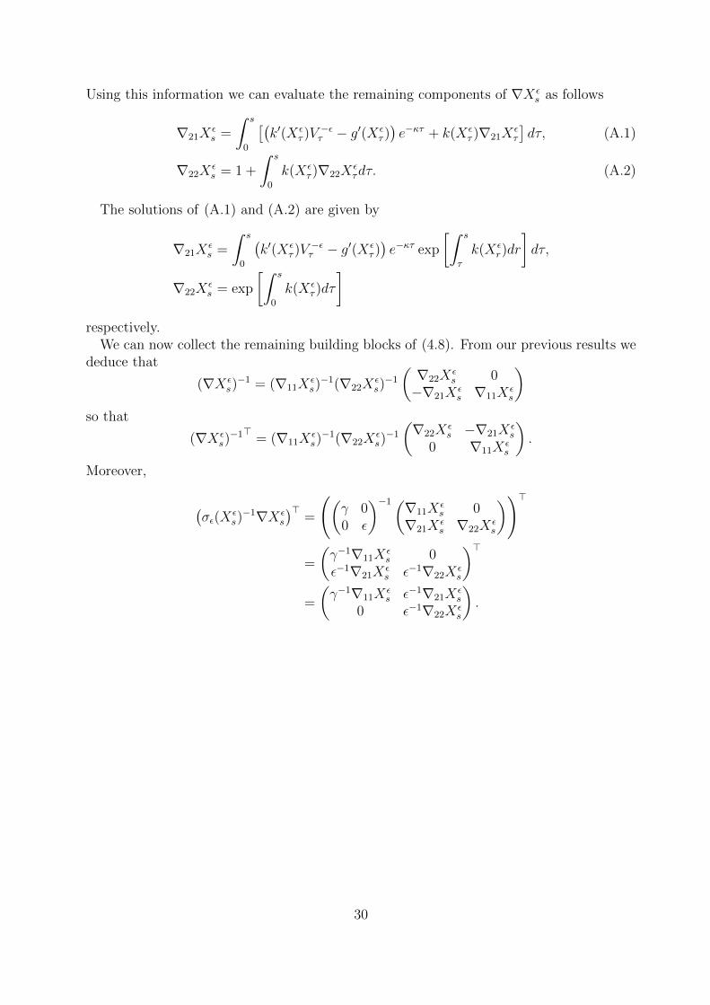
Using this information we can evaluate the remaining components of ∇Xεs as follows

∇21Xεs =

∫ s

0

[(k′(Xε

τ )V−ετ − g′(Xε

τ ))e−κτ + k(Xε

τ )∇21Xετ

]dτ, (A.1)

∇22Xεs = 1 +

∫ s

0

k(Xετ )∇22X

ετdτ. (A.2)

The solutions of (A.1) and (A.2) are given by

∇21Xεs =

∫ s

0

(k′(Xε

τ )V−ετ − g′(Xε

τ ))e−κτ exp

[∫ s

τ

k(Xεr)dr

]dτ,

∇22Xεs = exp

[∫ s

0

k(Xετ )dτ

]respectively.

We can now collect the remaining building blocks of (4.8). From our previous results wededuce that

(∇Xεs)−1 = (∇11X

εs)−1(∇22X

εs)−1

(∇22X

εs 0

−∇21Xεs ∇11X

εs

)so that

(∇Xεs)−1> = (∇11X

εs)−1(∇22X

εs)−1

(∇22X

εs −∇21X

εs

0 ∇11Xεs

).

Moreover,

(σε(X

εs)−1∇Xε

s

)>=

((γ 00 ε

)−1(∇11Xεs 0

∇21Xεs ∇22X

εs

))>

=

(γ−1∇11X

εs 0

ε−1∇21Xεs ε−1∇22X

εs

)>=

(γ−1∇11X

εs ε−1∇21X

εs

0 ε−1∇22Xεs

).

30