Dynamics of smallholder participation in horticultural export chains

–Evidence from Ecuador-

By Cristina Romero* and Meike Wollni,

Department of Agricultural Economics and Rural Development and Research Training Group

“GlobalFood”, University of Göttingen, Platz der Göttinger Sieben 5, 37073 Göttingen, Germany

In this paper we study the dynamics of smallholder participation in export value

chains focusing on the example of small-scale broccoli producers in the highlands of

Ecuador. We analyze the extent of participation over an 11-year time period using

correlated random effects and diff-GMM models and explain the hazards of dropping

out of the export chain based on a multi-spell cox duration model. The empirical

results suggest that small-scale farmers' exit from the export sector is accelerated by

hold-ups experienced in the past and that family ties play an important role in

farmers' marketing decisions. Negative external shocks – such as the global financial

crisis starting in 2007 that was associated with the bankruptcy of the main buyer in

our case study – represent a major threat towards the sustainability of smallholder

inclusion in high-value chains.

Acknowledgement: The financial support of the German Research Foundation (DFG) is gratefully

acknowledged.

1. Introduction

During the past three decades the agri-food industry has undergone rapid structural changes. The

growing demand for innocuous and high quality food has led to the modernization of

procurement systems inducing a shift from spot market transactions to vertical coordination

(Reardon et al. 2009). These structural supply and demand side changes have opened up new

marketing opportunities for small-scale farmers in developing countries. Farmers' inclusion in

global agri-food markets through producer groups and contract farming schemes is often

considered a promising way to increase farm incomes and thus foster rural development (Braun,

Hotchkiss, and Immink 1989; Kydd et al. 2004; Hernández, Reardon, and Berdegué 2007;

Maertens and Swinnen 2009). Based on the argument that participation in high-value markets

can provide an avenue out of poverty in rural areas, promoting and linking small farmers to these

markets has become a main focus of donors and NGOs in recent years (Altenburg 2006).

While the export of fresh products from developing to high-income countries has increased over

the past decades, smallholders often face major barriers in their access to high-value markets

(Dolan and Humphrey 2000; Henson et al. 2005; Schuster and Maertens 2013). An extensive set

of literature dealing with the determinants of smallholder participation in modern food markets

offers mixed results. Berdegué et al. (2005), Dolan and Humphrey (2000), Reardon et al. (2007),

Schuster and Maertens (2013), and Rao and Qaim (2011) show evidence for the exclusion of

small-scale farmers from high-value markets and reveal that export companies or local

supermarkets source only a small percentage of their produce from smallholders. In contrast,

Bellemare (2012), Henson et al. (2005), Maertens and Swinnen (2009), Minten et al. (2009),

Reardon et al. (2009), and Schipmann and Qaim (2010) describe successful cases of smallholder

inclusion that rely on institutional innovations, such as contract farming schemes.

While these studies provide some evidence on the determinants of participation at a particular

point in time, little research has been done on the sustainability of smallholder inclusion in high-

value chains over time. This is of particular relevance as some evidence suggests that contract

farming schemes regularly lose participants or collapse entirely (Barrett et al. 2012). Therefore,

the dynamics of participation may be much more complex than suggested by cross-sectional

studies and may also explain to some extent seemingly contradictory results. A few recent

studies have investigated the dynamics of market participation focusing on domestic

supermarkets in Kenya (Andersson et al. 2015), export-related standard adoption in Thailand

(Holzapfel and Wollni 2014), and the disadoption of horticultural export crops in Guatemala

(Carletto et al. 2010). However, due to the difficulty of obtaining consistent data on farmers'

marketing choices over several years, these studies rely on two-year panel or recall data. These

data are usually too short or not precise enough to reveal the complex dynamics of (multiple)

entries and exits from a high-value chain and the relative importance of transaction risks for

contract performance.

The aim of this study is to address this research gap by analyzing the factors influencing

smallholders' decision to deliver their produce to the export market as well as the decision to

remain a supplier or to drop out temporarily or permanently from the export chain. We place

particular emphasis on the role of transaction risks (i.e. payment delays and product rejections)

that may influence and shape the farmers' marketing decisions. We thus investigate the effects of

household characteristics and past experiences in the supply chain on the extent of participation

(measured in terms of the quantity delivered to the export chain). Furthermore, we analyze the

determinants of withdrawal from the export chain, taking into consideration that farmers may

enter and exit the chain multiple times.

Our analyses are based on a unique data set consisting of original household survey data

collected in 2012 and the records of a collection center to which all broccoli from small-scale

farmers destined for the export market is delivered. The records of the collection center contain

transaction level information for every transaction of all the suppliers during the past eleven

years (i.e. since it was established). Our data shows that a large percentage of small-scale farmers

do not participate continuously in the high-value export market channel, but instead decide to

abandon it temporarily or completely and return to the local market. Using panel data we can

investigate the dynamic relationships within the supply chain while controlling for unobserved

heterogeneity of farmers and for yearly shocks that may affect production levels (e.g. weather

shocks, price shocks, etc.).

The article is organized as follows. The next section gives background information on the

broccoli sector in Ecuador. The third section discusses the conceptual framework for the

empirical analysis. Section four provides information on data collection and develops the

econometric models. Finally, section five and six present the results and section seven concludes.

2. The broccoli market in Ecuador

Broccoli was introduced as a crop in Ecuador in the 1990's and since then its cultivation has

spread rapidly until it became the country's second most important non-traditional export

product. In 2008, Ecuador became the 6th

largest exporting country of broccoli and cauliflower

(5th

in value exported) with around 60 thousand tons sent to North American and European

markets representing around 57 million dollars (FAOSTAT, 2013). However, in the following

years exports started to decrease, and by 2010 Ecuador was relegated to the 11th

place (34

thousand tons and 35.5 million dollars). Figure 1 presents export prices and quantities of broccoli

and cauliflower1 since 1992, showing a constant and significant increase in quantity until 2009

and after that a constant drop until present times (National Central Bank, 2013)2. During the

1 Data for broccoli alone are not available.

2 The price/ton depicted in the graph was obtained dividing total broccoli and cauliflower exported per year by total

income received obtained from national statistics. Therefore, it is the average of the price obtained in the

same time, prices have been relatively stable spiking in 1996 and then again since 2007 showing

an increasing tendency.

FIGURE 1

Initially, broccoli was only cultivated on large plantations and exported by a few processors, but

since the year 2001 small-scale farmers from the Chimborazo province3 were linked to the export

market. A few years later, small-scale farms4 represented one-third of the total broccoli area

planted for the international market and the remaining two-thirds were cultivated by medium and

large-scale farms as well as by the same exporting firms in vertically integrated production units5

(Gall 2009).

Small-scale farmers were linked to the export market through a producer organization that served

as an intermediary between farmers and the export firm. The producer organization established a

collection center in the village in order to assemble the broccoli and send it to a private

processing-exporting firm (from here on referred to as exporter). This firm cut the broccoli into

small pieces, froze it and exported it to international markets. The first eight months only

members of the association supplied the export sector through the collection center. Over the

following years, the number of members of the association remained constant and no new

members were admitted. However, hundreds of producers from neighboring villages joined the

chain as suppliers6.

Between the exporter and the producer organization a written contract was signed, in which the

volume, a fixed price, quality and payment conditions were specified. The producer organization

relied on verbal agreements with smallholder farmers regarding the quantity and quality

specifications of broccoli deliveries. A typical production contract system was put into operation

with the exporter providing the plants through the collection center and facilitating access to

inputs, credit, market and technical information. The farmers on the other hand were in charge of

growing broccoli on their land under the firm's technical direction and had to deliver the product

to the collection center in order to pay for the services received.

international market, which increased over the years, but it does not necessarily represent the price paid by exporting

firms to local producers. 3Small-scale farmers were supported by a local NGO to form a producer group and produce broccoli for the export

market. 4 Defined as farmers owning less than 20 ha (Gall, 2009).

5 Large and medium scale plantations are located in the province of Cotopaxi and were not included in our analysis.

6 For more insights on the advantages of working with smallholders in this specific case refer to Gall (2009).

In summary, the broccoli harvest and post-harvest process consists of the following stages: i)

prior to the harvest, the farmer has to decide where to sell his product according to its quality,

which is assessed by a collection center's worker, ii) the broccoli going to the export sector is

delivered to the collection center, where it undergoes a first grading process in the presence of

the farmer, iii) the broccoli meeting the quality criteria at the collection center is further sent to

the exporter, where a second grading process takes place, this time in the absence of the farmer7.

Until 2010, the broccoli from different farmers was sent to the exporter in separate bins. As the

overall quantity delivered by smallholders has decreased, the broccoli from different producers is

nowadays mixed in the same container and sent to the firm. Therefore, since 2010 the quantity

rejected by the exporter is divided equally among the farmers who sent their product with that

specific shipment (on average one truck is dispatched every working day from the collection

center to the firm). Finally, iv) the product meeting the exporting firm's quality requirements is

accepted and the payment is made two weeks later according to the terms of the contract. Due to

the fact that broccoli for the export market is harvested differently than that for the local market

and due to its high perishability, the broccoli rejected at the exporter level can no longer be sold

in the local market and thus represents a monetary loss to the farmer8.

Nowadays, twelve years after the inclusion process started, a large percentage of small-scale

suppliers have abandoned the scheme and the collection center faces a shortage of broccoli

supplies. In consequence of the global financial crisis starting in 2007, the export broccoli chain

underwent a major crisis in 2009, when the exporting firm sourcing from the collection center

went bankrupt and left the scene without paying for the product delivered over several months.

As a consequence, the collection center faced a liquidity crisis, and payments to farmers were

delayed for extended time periods. Formal legal institutions have not solved the problem so far

and the farmers' collection center still has a large debt to recover from the exporter. After their

original buyer went out of business, the farmers' collection center established a new marketing

contact with one of the remaining broccoli processors-exporters in the country. This exporter

agreed to source from the collection center to supplement its own estate production. The contract

scheme outlined above still applies in this new marketing relationship, and is re-negotiated on an

annual basis.

In personal interviews, the exporters have emphasized the existing demand for Ecuadorian

broccoli in the international market and the constant need for new and efficient suppliers given

land constraints that hinder the expansion of their own plantations. Yet, they have also pointed

out their reluctance to work with smallholders because of the associated coordination problems,

especially since there is a shortage of suppliers. When the collection center was booming with

7 The rejection data in our data set refer to the rejections at the exporter level, and do not take into account rejections

at the collection center where the farmer can assist and verify the process. 8 When harvested for the export market only the head of the broccoli is cut and the rest of the plant is left in the

field, while for the intermediaries and local market the head has to be covered by several plant leafs.

suppliers, trucks were filled faster and dispatched to the processing plant immediately. In

addition, traceability was easier to implement since the broccoli from different farmers could be

kept in separate bins. Nowadays, it takes longer for the truck to fill and the waiting time affects

the quality of the product. Moreover, planning is difficult, because the exporter cannot rely on

certain volumes being delivered by the collection center.

Fig. 2 shows the dynamics of broccoli supplies to the collection center during the last decade.

The amount of broccoli delivered to the export sector drastically declined in 2009 and since then

has been further decreasing. Suppliers have joined and abandoned the supply chain at different

points in time. The total number of farmers who have ever participated in the export sector is

around 630 from eight different villages located in the province of Chimborazo. The largest

number of suppliers (403 smallholder farmers) was registered in 2005. Nowadays, there are only

108 active suppliers of which only 47 are members of the producer organization.

FIGURE 2

3. Conceptual framework

Broccoli producers in Ecuador can choose between two alternative marketing channels to sell

their produce: 1.) The spot market: coordinated by price and characterized by nonrecurring

transactions with no prior arrangements and no promise of repeating the transaction in the future.

It takes place at the local market or at small market points close to each community. There are

multiple buyers and multiple sellers and payment is usually made at the moment of the

transaction. 2.) The export market: characterized by vertical coordination between the parties to

supply a fixed quantity of broccoli with certain characteristics, during a certain time period and

at a constant price. The payment is usually made 15 days after delivery and the closer

relationship between the parties can facilitate the flow of information. While large-scale farmers

are offered individual contracts directly with the exporting firm, small-scale farmers can only

access the export market through verbal agreements with the collection center managed by the

farmers' group under study.

In order to participate in the export marketing channel, farmers have to fulfill stringent

requirements related to the quality, quantity and timing of deliveries. The farmer's ability to meet

these conditions determines the probability and extent of participation. In principle, we assume

that farmers decide to participate in the export market if their utility derived from participation is

higher than their utility derived from non-participation, or in other words, higher than their

opportunity costs of participation (Barrett et al. 2012). The farmer's utility associated with

participation in the export chain is influenced by several factors including revenues and

production costs as well as the transaction risks associated with selling broccoli in the export

sector. Based on the framework proposed by Williamson (1979) and extended by Hobbs and

Young (2000), Table 1 summarizes the transaction risks associated with the commercialization

of broccoli in the export chain compared to the alternative, i.e., the local market.

TABLE 1

While certain types of risks are typically reduced through contract farming arrangements that

link smallholders to export markets similar to the one studied here, other types of risks can be

exacerbated (Barrett et al. 2012). Uncertainty related to the price and to finding a suitable buyer

is usually lower compared to transactions in the local market, given that a purchase agreement

exists with a secure buyer and the price is negotiated ex-ante, thus allowing farmers to plan

production costs accordingly. However, new uncertainties may be introduced, e.g., related to the

farmer's ability to meet strict quality requirements. Furthermore, even though an ex-ante

agreement exists, the exporter may renege on the agreement9, e.g. by rejecting produce

inappropriately or by delaying or defaulting on the final payment10 (Barrett et al. 2012). When

high quality requirements are defined, as in the export market, uncertainty surrounding the

compliance with these quality criteria increases (in particular when criteria are difficult to

determine objectively and depend on subjective assessment). As a result, the grading process,

often performed in the absence of the farmer, is characterized by asymmetric information and

can be susceptible to opportunistic behavior (as reported e.g. by Saenger et al. 2014).

Furthermore, the threat of opportunistic behavior is exacerbated by relationship-specific

investments incurred by farmers producing for the export market. In the broccoli sector, these

become especially relevant after harvest, due to distinct harvesting technologies between the two

markets. Thus, once the product has been harvested for the export market, the farmer is locked

into the marketing relationship with the exporter, given that his second best option of marketing

the broccoli elsewhere now tends towards zero11. We expect that the realization of these

transaction risks, i.e., to what extent the exporter takes advantage of holdup opportunities,

determines the gains accruing to farmers, and thus, in the long term the dynamics of smallholder

participation in the export market. In particular, past holdups experienced by the farmer threaten

the sustainability of the chain by reducing the farmer's willingness to invest, and thus the

9 This refers to both situations in which the exporter is experiencing a negative shock and is therefore unable to

fulfill his contract obligations as well as situations in which the exporter is behaving opportunistically. 10

When payments are delayed, the contracting firm is effectively extracting rents from its suppliers by getting

access to interest-free loans. Suppliers on the other hand experience economic losses and can face cash-flow

shortages, especially if they are credit-constrained. 11

In the local market, asset specificity is lower, because multiple buyers exist. Accordingly, even if one buyer turns

down the produce, other equally good marketing options exist in the spot market.

quantity of produce delivered, and – if transaction risks become too high – can even induce a

farmer to drop out of the export market entirely.

4. Empirical Analysis

4.1. Data collection

In order to disentangle the dynamics of small-scale farmers supplying the export market we

collected quantitative as well as qualitative data on the marketing decisions of broccoli producers

in Ecuador. Qualitative methods were used to collect general information on broccoli production

and on the organization of the broccoli sector in the province of Cotopaxi – where the processing

firms and large-scale farms are located – and in the province of Chimborazo. In a first step, we

conducted semi-structured interviews with members of the farmers' group, exporting firms and

government entities supporting inclusive business12 in order to understand the structure of the

sector, its development since the 90's and the current state of the value chain. Subsequently,

quantitative research was carried out in the province of Chimborazo, where the small-scale

farmers are located. The farmers' association under study is the only organized group of

smallholders producing broccoli for the export sector in the country. It has supplied exporting

firms through contract farming for over a decade13. A household survey was carried out from

November 2012 to February 2013 in nine villages of the province of Chimborazo. We covered

all eight villages where former and active suppliers of the collection center live. In addition, we

interviewed farmers who never participated in the export market living in the same eight villages

and from a ninth village located in the same province (with the same infrastructure and climatic

characteristics).

Three categories of farmers were identified for the analysis: Active suppliers of the export

market (current participants, n=108), former participants who stopped supplying the export

market channel (former participants, n=522) and farmers who have always supplied the local

market (non-participants, n= approx. 1500). A stratified random sample was used to select

farmers for the interviews. Given their comparatively small number, we decided to over-sample

current suppliers in order to ensure sufficient observations for analysis. Current and former

participants were randomly chosen from a complete list of active and former producers provided

by the association. If producers were not available or did not agree to participate in the

interviews, they were replaced with the next person on the list. Non-participants were selected

using a random walk sampling approach. In order to obtain a comparable control group,

households were chosen only if they have been producing broccoli during the last 12 months.

12

The main purpose of inclusive business is to link small/poor producers to the market in a sustainable way. 13

Nowadays, smallholders can only access the export chain through a farmers' group given that firms do not sign

individual contracts with small-scale producers. Sporadic participation in the export chain of non-organized small-

scale suppliers was possible during the 90s and early 2000s.

The final sample is composed of 401 farmers: 88 farmers who still participate in the export

chain, 195 farmers who have dropped out of the scheme, and 118 farmers who have always

grown broccoli exclusively for the local market. A structured questionnaire was used to collect

information on socio-economic and farm characteristics, agricultural production and marketing,

group memberships, family ties and household assets. Information on farm size and on family

members who have worked in the collection center was obtained for the past eleven years using

recall data. The respondent's attitude towards risk was measured using an experimental risk

lottery designed by Binswanger (1980), where real payoffs were offered. Enumerators visited

each household and conducted a face-to-face interview of approximately 1.5 hours with a

household member involved in the cultivation and commercialization of broccoli. The data

collected for the current and former suppliers of the export chain was merged with records

provided by the farmers' association containing data on the quantity of broccoli delivered from

2002 to 2012, the days to payment, and the quantity rejected by the exporter per delivery.

4.2. Model specification

4.2.1. Extent of participation

Each year farmers have to decide how much of their broccoli they allocate to the export sector

and how much they sell in the local market. We model this marketing decision by analyzing the

factors influencing the extent of participation in the export chain specifying the following model:

𝑄𝑖𝑡 = 𝛼𝑄𝑖(𝑡−1) + 𝛽𝑇𝑅𝑖(𝑡−1) + 𝜃𝑿𝑖𝑡 + 𝜋𝒁𝑖 + 𝑐𝑖 + 𝜇𝑖𝑡

The extent of participation is measured as the quantity Q that farmer i delivers to the export

market in year t14. Qit is specified as a function of previous deliveries Qi(t-1), the transaction risks

experienced by the household in the previous period TRi(t-1), a vector of other time variant

covariates Xit, and a vector of time invariant covariates Zi potentially influencing the marketing

decision. The error term is composed of a time constant unobserved heterogeneity term (ci)

reflecting the unobserved characteristics of each individual (e.g. management ability, motivation,

cognitive ability, etc.), and a time varying error term (μit), which reflects external shocks that are

non-systematic. If the farmer does not deliver any broccoli to the export market during a specific

year, Qit is set to zero, i.e. the observation enters the analysis. However, transaction risks are not

observed during years in which the farmer does not participate in the export market, resulting in

missing values in the subsequent year, and thus giving our panel an unbalanced structure.

There are three potential sources of endogeneity in our estimation: i) The decision to participate

each year may be correlated with the constant unobserved characteristics of each individual (ci)

(e.g. loyal individuals may participate more consistently, while others decide to participate only

14

Qit equals zero if the farmer does not deliver any broccoli to the export market in a specific year.

sporadically). ii) ci may be correlated with the independent variables (e.g. the motivation of a

farmer can influence the quantity delivered to the export sector, but also the quality of the

broccoli and thus the quantity rejected). iii) Controlling for persistence in supplying behavior

may cause endogeneity, because the lag term of the dependent variable Qi(t-1) is likely to be

positively correlated with the error term (due to ci) (Bond 2002). Even though we are not

interested in the effect of Qi(t-1), Bond (2002) states the necessity to control for possible

autoregressive dynamics in order to obtain consistent estimates of the remaining parameters. We

propose two estimation techniques to address these problems: a) a Correlated Random Effects

model for unbalanced panel data to control for unobserved heterogeneity (ci), and b) a First-

Differenced General Method of Moments model, which eliminates ci and controls for the

endogeneity of Qi(t-1).

Correlated random effects (CRE) model for unbalanced panels

With panel data, one way of controlling for time constant unobserved heterogeneity (ci) is to use

Fixed Effects estimators. This removes, however, all time constant explanatory variables (Zi)

from the analysis, which are often of interest for understanding the drivers and barriers to

participation. This disadvantage can be overcome using the Mundlak-Chamberlain approach,

which controls for fixed effects by including a correlated random effects (CRE) estimator.

Wooldridge (2010) show that this method is also valid for obtaining unbiased estimators with

unbalanced panels, as long as we can assume that selection is not correlated with the time

varying error term (μit).

The CRE model allows for linear correlation between the unobserved heterogeneity term ci and

the observed explanatory variables by including a vector of variables containing the means of all

time-varying covariates for each household as indicated in the following equation:

𝑄𝑖𝑡 = 𝛼𝑄𝑖(𝑡−1) + 𝛽𝑿𝑖𝑡 + 𝜋𝒁𝑖 + 𝜉𝑋�̅� + 𝑎𝑖 + 𝜇𝑖𝑡

where Xit contains all time-varying covariates including TRi(t-1), and 𝑋�̅� is a vector of variables

containing the means of the time-varying covariates including the time dummies (Wooldridge

2010). In unbalanced panels, the calculation of means is based only on the selected observations

that enter the estimation in the specific year (Wooldridge 2010). With this approach we

eliminate the problem of self-selection based on ci and the endogeneity caused by possible

correlation between covariates and ci. The model is estimated using Random Effects and

standard errors are clustered at the household level to obtain estimates robust to

heteroskedasticity and correlation among the disturbances as recommended by Wooldridge

(2010).

Generalized Method of Moments

The second estimation strategy is First-Diff GMM developed by Arellano and Bond (1991). It

uses first differences to eliminate the unobserved heterogeneity term (ci) and an instrumental

variable approach to eliminate the endogeneity of the lagged dependent variable (Qi(t-1)). For this

purpose, further lags of Qi(t-1) in levels are used as instruments. The final model to be estimated is

specified in the following equation:

∆𝑄𝑖𝑡 = 𝛼∆𝑄𝑖(𝑡−1) + 𝛽∆𝑿𝑖𝑡 + ∆𝜇𝑖𝑡 |𝛼| < 1

where ΔXit contains all differences of the time-variant covariates including TRi(t-1). First

difference GMM is expected to perform poorly if the series used in the estimation are random

walks or highly persistent (Bond 2002). A necessary assumption for the model is that the time-

varying errors are not serially correlated. This implies that Qi(t-2) and past lagged levels are not

correlated with Δμit and therefore can be used as instruments for ΔQi(t-1). The assumption of no

serial correlation is fulfilled if there is no second-order serial correlation in the first-differenced

residuals15. The validity of the instruments can be tested using the Sargan test of over-identifying

restrictions.

An indication of the consistency of α can be obtained by comparing the first-differenced GMM

results with those obtained with OLS and Fixed Effects. Since Qi(t-1) is correlated with the

individual effects (ci), the OLS estimate is expected to be biased upwards. On the other end, the

Fixed Effects estimate will be biased downwards, because of the negative correlation introduced

between the transformed lagged dependent variable and the transformed error term. Therefore, a

consistent estimator of α is expected to lie between the ones obtained with OLS and FE (Bond,

Hoeffler, and Temple 2001; Bond 2002).

4.2.2. Dropping out of a high-value chain

Time duration models estimate the probability that an individual switches from one stage to

another given that he has not done so in the previous period (Dadi, Burton, and Ozanne 2004).

We model the farmer's decision to withdraw from the export marketing channel, by estimating

the probability that the farmer changes his position from participation to non-participation at the

beginning of time period t, given that he has not done so before t. We organize our data in a

discrete time fashion, where each farmer has eleven observations, one for each year of the time

period under study (2002 – 2012). Given that the withdrawal from the export sector is

conditional on previous participation, we exclude those farmers who never participated in the

export sector from the analysis. The event of withdrawal is called failure, and we denote the

discrete time to failure with T. The dependent variable is a dummy variable that equals zero in

15

First order serial correlation is expected in the first-differenced residuals even if the disturbances are serially

uncorrelated. When using System GMM, second order correlation is present, therefore we limit our model to using

only Difference-GMM.

every year that the farmer supplies the export sector and one in the year he stops supplying

(failure). Multiple spells are allowed, which means that farmers can decide to participate a

second or third time after withdrawing. The spell or time of duration starts when the farmer starts

supplying the export market and finishes when he decides to withdraw. A vector of time variant

covariates (Xit) is included, which is fixed within the interval t and speeds up or delays the

failure time of the individual. A vector of time invariant covariates (Zt) is also observed, which is

constant over the whole period under study.

The hazard function (αi), which characterizes T, is given by the conditional probability for the

risk of failure in interval t (Fahrmeir 1997) given that the individual has not failed before t and is

expressed by:

αi(t|Xit, 𝑍𝑡) = Pr(Ti = t|Ti ≥ t, Xit, 𝑍𝑖) , t = 1, … , q

Where Ti = t denotes failure within interval t, Ti ≥ t denotes survival up to time t for individual i,

Xit is a vector of time varying covariates including TRi(t-1), and Zi is a vector of time invariant

covariates.

The hazard function can also be expressed as a function of time (baseline hazard) combined with

a vector of covariates acting multiplicatively on the baseline hazard and shifting it proportionally

(Burton, Rigby, and Young 2003). Semi-parametric approaches in duration analysis, such as the

Cox model, do not require any assumption on the distribution of the errors, and thus of the

baseline hazard. Instead they rank the occurrence of failures and conduct a binary analysis on

each observation, exclusively using the ranking of survival times (Cleves et al., 2008). The

proportional hazard model, which we will estimate using the Cox model approach, is specified

as:

𝛼𝑖𝑗(𝑡) = 𝛼0(𝑡)𝑒𝑥𝑝(𝛽𝑋𝑖𝑗 + 𝛾𝑍𝑖 + 𝑣𝑗)

Where α0(t) is the unspecified baseline hazard, 𝑣𝑗 corresponds to the error term (frailty) of the

model, i.e., a latent random effect within groups that enters multiplicatively on the hazard

function. Given that in our data we have multiple observations per individual (multiple spells),

we can expect that the failing times for each farmer are not independent from each other and thus

the standard errors should be adjusted to account for this possible correlation. The option of

shared frailty is used to account for this potential correlation, which is measured by θ and is

assumed to have a gamma distribution (Cleves et al., 2008). As we consider time discrete (yearly

data), it is likely that more than one observation fails at the same time (tied failures) and as a

result the order of failures within this year cannot be established as required for the simple Cox

model. Cleves et al. (2008) mention three ways of handling such tied failures, of which we use

the Efron's method16.

4.2.3. Potential determinants

Among the variables potentially explaining the extent of participation as well as the decision to

drop out of the export sector, we are particularly interested in the effect of transaction risks. In

particular, hold-ups experienced in previous periods might increase the perceived risk of the

transaction and thus have a strong negative effect on participation. Transaction risks are captured

by the variables: a) payment delay(t-1) which is the average number of days the farmer had to wait

for payment from the exporter in the previous year, and b) log_kg rejected(t-1) which represents

the total kilograms rejected by the exporting firm in the previous year in logs17. We consider

these variables strictly exogenous, which means that feedback from current or past external

unobserved shocks has been ruled out.

Regarding other transaction characteristics, the price per kilogram paid by the exporter to the

collection center at time t is included in the model (price export market). This value represents a

fixed price that is negotiated between the farmers' group and the exporter on an annual basis. In

addition, we include a dummy that equals one if during 2012 the average price obtained by the

farmer in the local market was below the fixed export market price of 2012. We use this variable

as a proxy for low bargaining power in the local market. As we only have farmer-specific local

market prices for 2012 and not for the full study period, we implicitly assume that individual

bargaining power remained invariable throughout the analyzed time period.

Furthermore, we consider three distinct proxies for social networks and information access. First,

we include a dummy variable that equals one if the farmer has family ties with workers of the

collection center. Given that family ties play an important role in Latin American rural societies

(Carlos and Sellers 1972), farmers may feel more obliged to meet their commitment and deliver

their produce to the collection center, if a family member is working there. On the other hand, for

the case of Madagascar, Fafchamps and Minten (2001) show that contracts are handled more

flexibly among kin and thus deviations from the original agreement are observed more

frequently. Second, we follow Moser and Barrett (2006) using the aggregate quantity delivered

per village (aggregate village supplies(t-1)) as a proxy for community behavior and expectations.

Moser and Barrett (2006) describe how the pressure to conform to behavioral norms established

16

Efron's method is an approximation to the exact marginal calculation method for tied failures, where all the

possible orders of failures within a group failing at the same t are taken into account for the final probability of

failure at that specific time t. In Efron’s method the risk set used as denominator contains all the observations failing

at time t, but is corrected using probability weights (Cleves et al. 2002). 17

In the duration model, we do not control for the total amount of broccoli delivered in the previous time period, and

therefore, instead of the absolute quantity rejected we include the percentage of produce rejected in the previous

time period.

within a community can affect individual decisions. Therefore, if many village members are

active suppliers of the export market and village leaders encourage participation, individual

farmers might associate higher social acceptance with that particular marketing channel. In

addition, higher levels of aggregate village supplies can also result in better access to information

and lower costs of transportation for individual farmers. In the econometric estimation we

consider this variable as pre-determined (it may be influenced by past external shocks) and use

lagged aggregate village supplies to minimize endogeneity problems resulting from reverse

causality. Third, membership in the farmers' group operating the collection center can facilitate

access to information, e.g. regarding the conditions of export market participation, and to the

services provided by the organization such as access to technical support and credit. In addition,

members made monetary contributions to the initial investments of the organization and

therefore have a stake in the business, which also makes them more likely to patronize the

collection center. It is important to note that farmers became members of the farmers’ group

when it was founded in 2001, and in the following years no new members were admitted.

While often unobserved in empirical studies due to the difficulty of measurement, we also

include the farmer's attitude towards risk as a potential determinant. This is particularly

important in the context of our study, given that the farmer's risk attitude is likely to influence his

subjective perception and evaluation of transaction risks. We played an experimental game with

real payoffs proposed by Binswanger (1980) to obtain a measure of risk attitude. Six different

gambling options were presented to each farmer at the end of the interview, each option with a

different partial risk aversion coefficient ranging from extreme risk-averse (if option 1 was

preferred) to neutral or negative risk-averse (if option 6 was preferred). Given that many of the

interviewed farmers were illiterate, for each of the six options we presented them a picture of the

sum of money they could win. The partial risk aversion coefficient was then calculated

according to the farmer's choice as explained in Binswanger (1980) and normalized to a scale

from 0 (low risk aversion) to 1 (high risk aversion). We expect that more risk-averse farmers

prefer the market channel associated with lower risk. Accordingly, risk-averse farmers may be

more likely to participate in the export chain offering them a secure market and a secure price.

On the other hand, if there is mounting evidence of increasing transaction risks, such as payment

delays or product rejections, risk-averse farmers may be the first to drop out of the chain.

To capture poverty, we use a dummy variable that equals one if the household received a

governmental cash transfer (cash transfer), which is targeted to the poorest households in the

country. Other variables capturing household and farm characteristics are included as controls,

such as age, gender and education of the household head, number of household members, lagged

farm size, and distance to the collection center in kilometers. In most specifications, we include

interaction terms between a dummy variable for the period 2009 – 2012 and our main variables

of interest in order to control for the time span after the negative external shock caused by the

bankruptcy of the buyer. Long payment delays and payment defaults during this time may have

jeopardized the trust of smallholder suppliers, negatively affecting their participation in the value

chain. Year and village dummies are also included to control for year-specific macroeconomic

effects and shocks as well as village-specific characteristics.

5. Descriptive results

Descriptive statistics for the covariates included in the models are presented in Table 2 as well as

in Table A1 in the Appendix. Table 2 compares the characteristics for the year 2012 of farmers

currently supplying the export market (current participants), farmers who dropped out of the

export market (former participants) and farmers who have never supplied the export market

(non-participants). Descriptive results indicate that while most of the household characteristics

do not differ significantly between the three groups, current participants have less education but

more farming experience than former participants and in particular than non-participants.

Geographically, current participants are located closer to the collection center and further away

from the local market, compared to both former and non-participants. We find no significant

difference in the size of owned land (in 2012) between the three categories of farmers; only when

taking into account rented and shared plots the total land size of non-participants is slightly

bigger than that of current participants (significant at the 10% level). Yet, current participants are

more specialized in terms of the area dedicated to broccoli production. Nevertheless, when

looking at the income derived from broccoli production, we find no significant difference

between the three groups. Furthermore, income differences, even though slightly lower for

current participants, are not significantly different between the groups. According to our proxy

for wealth (cash transfer), however, we do find evidence that current participants are

significantly poorer than non-participants. Finally, we find significant differences between the

groups with respect to social networks. A significantly larger share of current participants is

member of the farmers' group and has family ties with workers at the collection center.

Compared to non-participants, both current and former participants have a larger number of

relatives producing broccoli for the local market and in particular for the export market.

Large differences also exist between the three groups of farmers regarding the characteristics of

the market transactions. First of all, we observe that only 22% of the current participants

exclusively sell their broccoli to the export market. The majority of current participants, besides

delivering to the export market, also deliver some of their produce to the local market. Yet, when

compared to former and non-participants, their income obtained from local market sales is

significantly lower, because some of their produce was destined to the export sector.

TABLE 2

With respect to the transaction risks, we can observe stark differences between the two

marketing channels. In the export market farmers had to wait on average 38 days for their

payment in 2012, whereas in the local market payment was made on average within two to four

days after delivery. Similarly, stringent quality requirements result in relatively high rejection

rates in the export sector. On the average, 11.5% of produce delivered by current participants

was rejected in the high-value chain, while in the local market produce rejections are not an

issue. In the export market, farmers received a fixed price of 0.25 US$/kg throughout the whole

year (of which the collection center kept 0.02 US$/kg to cover their costs), but in the local

market farmers faced extremely volatile prices ranging from 0.04 US$/kg to 1.43 US$/kg (mean:

0.40 USD/kg, standard deviation: 0.24).

When current and former participants were asked about the problems experienced in the export

sector, over 70% reported payment delays and 30% mentioned that they were not paid at all,

because the exporter defaulted on the payment (see Figure 3). Furthermore, around 35%

experienced produce rejections. This reflects the high levels of uncertainty to which farmers in

the export sector are exposed. Both delayed/lack of payment as well as produce rejections

negatively affect the cash flow and/or income of smallholder farmers, which often do not possess

the means and liquidity to compensate such losses. Finally, low prices and high quality

requirements were considered a problem by 25% and 10% of the current and former participants,

respectively.

FIGURE 3

In spite of the perceived problems, over 60% of the entire sample (including non-participants)

would be willing to produce broccoli for the export market and join a contract scheme, if it was

supported by a legal document18 (Figure 4). The conditions that are critical for them to sign an

agreement include secure payment (85%) and higher prices (50%). Less than 16% of the farmers

mentioned the provision of inputs, training or credit as a condition to participate in the export

market, thus providing some evidence for the existence of functioning factor markets in the area.

FIGURE 4

18

No particular buyer was specified in the question.

6. Econometric results

When investigating the determinants of the quantities delivered to the export market or the

factors influencing the withdrawal from the export chain, those farmers who never participated in

the export chain (non-participants) are not considered in the analyses, given that participation is

a pre-requisite for the subsequent decision of product allocation and withdrawal from the chain19.

Nonetheless, we are interested to know whether there are systematic differences between those

farmers who at some stage supplied the export market and those farmers who have never done

so. To test for potential selection bias, we estimate a Heckman selection model based on the full

sample (non-participants, former and current participants). In the first stage, a probit model is

used to predict the probability of ever participating in the export market. In the second stage, for

those farmers who have ever supplied the export sector the quantity delivered during their first

year of participation is predicted. Estimation results are reported in Table A3 in the appendix.

Rho is not statistically significant, indicating that sample selection is not an issue and farmers

who participate in the export sector are not systematically different from those who supply the

local market. In the following sections, those farmers who have never entered the export sector

are not further regarded in the analyses.

6.1. Extent of participation

Table 3 presents the estimates from the Correlated Random Effects and First-Differenced GMM

models on the determinants of the extent of participation. Models (1) and (2) include interaction

terms of various potential explanatory variables with the time dummy 2009-2012 to control for

the possibility of a structural break induced by the external financial shock. For comparison,

columns (3) to (5) report additional model specifications and alternative estimators. Column (3)

provides CRE estimates without interaction effects. Comparing results in columns (2) and (3)

illustrates the importance of controlling for the structural break that is associated not only with

changes in the magnitude but even in the sign of several coefficients before and after the external

shock. Accordingly, the data provides strong evidence that supply patterns were adjusted in

response to the crisis. Finally, OLS and Fixed Effects estimates are reported in columns (4) and

(5).

TABLE 3

19

In the model on the extent of participation, non-participants could enter the analysis by setting their amount

delivered equal to zero. However, if they never participated in the export chain, they never experienced any

transaction risks and accordingly drop out of the analysis due to missing values. Setting their transaction risk values

equal zero would be misleading, because it suggests that they experienced no problems, when in reality they simply

did not perform any transactions in the export sector.

In the Diff-GMM model (column (1)) we address the endogeneity of the lagged dependent

variable kg delivered(t-1) by using lags two to five as instruments. A Fisher-type unit root test for

panel data rules out the existence of random walks in the series used in the model confirming its

validity (results are reported in Table A4 in the appendix). The Sargan and Hansen tests also

show that the instruments used are exogenous to the lagged dependent variable and therefore

valid for the estimation (results are reported in Table A5 in the appendix). Additionally, we find

no autocorrelation of second order in the model using the Arellano-Bond test for

autocorrelation20. Autocorrelation of first order is expected in first differences because Δµt and

Δµt-1 share a common term (results are reported in Table A6 in the appendix). Controlling for

potential endogeneity, the Diff-GMM estimates show that the amount of broccoli delivered in the

previous period has a significantly positive effect on the amount of broccoli delivered in the

current period. The coefficient estimate obtained from the Diff-GMM model lies between the

OLS and Fixed Effects estimates, which confirms its consistency. The path dependency or

persistence of deliveries reflected in this coefficient is in line with other studies that have

reported a strong positive correlation between lagged and current horticultural export volumes

(e.g. Schuster and Maertens (2015) for the Peruvian asparagus sector).

Regarding transaction risks, we find – consistently across both models (columns (1) and (2)) – a

strongly negative effect of past produce rejections on the extent of participation. According to

the CRE model estimates, a one percent increase in the amount rejected in the previous year

leads to a decrease in current deliveries of 4.6 kg. This effect is even further exacerbated by the

crisis, after which a one percent increase in rejection rate is associated with a decrease in the

delivered quantity by 17.6 kg. Once we adequately control for the endogeneity of lagged product

deliveries, the Diff-GMM model predicts an even stronger effect of product rejections ranging

from a reduction in deliveries of 23.3 kg before the crisis to 32.7 kg after the crisis. Regarding

payment delays, results are also consistent across both models, indicating a negative effect that is

statistically significant at the 10% level. Accordingly, each additional day of payment delay in

the previous period decreases current product deliveries by 9.8 kg. The effect of payment delays

on product deliveries remains unaltered after the external shock.

The CRE model further allows us to investigate the relationship between potential time-invariant

determinants and the extent of participation. First of all, a strong and significantly positive

correlation is identified for membership in the farmers’ group. On the average, membership

increases deliveries by as much as 1758 kg compared to non-members. This positive effect,

however, reverses with the event of the negative external shock to the supply chain. After the

crisis, members on the average deliver 1469 kg less to the collection center than non-members.

This may be due to members having better access to information regarding the performance of

the organization and thus being more aware of the difficult situation faced by the supply chain

20

The existence of autocorrelation of second order would invalidate the use of lags as instruments.

and reacting accordingly by reducing their produce allocated to the export market. Besides

membership in the farmers’ group, the other social network variables (aggregate village

supplies21 and family ties) do not seem to play an important role in farmers’ product allocation

decisions among alternative market outlets.

Finally, we observe that the quantity delivered increases with farm size, and that poor farmers

deliver significantly less compared to non-poor households. These relationships are affected,

however, by the negative external shock. After the supply chain is struck by the crisis in 2009,

farmers with larger farm sizes reduce their produce allocation to the export market, even though

the overall effect of farm size remains positive. On the other hand, the difference between poor

and non-poor farmers becomes insignificant in the post-crisis period (joint significance of the

coefficients on cash transfer and the interaction term: p= 0.1327). Finally, farmers with higher

risk aversion respond to the crisis delivering significantly less compared to farmers with low risk

aversion in the post-crisis period.

6.2. Dropping out of a high-value chain

Table 4 shows estimation results from the Cox model of proportional hazards analyzing the

decision of current and former participants to exit the export market. The coefficients represent

the change in the log odds of the outcome variable for a one-unit increase in the independent

covariate, holding all other covariates constant. For easier interpretation, the hazard ratios are

also provided, which were calculated by exponentiating the coefficients. A negative coefficient

implies a negative change in the log odds of the outcome variable, which means a decrease in the

hazards of dropping out of the export sector (hazard ratio < 1). On the contrary, a positive

coefficient reflects an increase in the log odds of the outcome variable, meaning an increase in

the hazards of dropping out (hazard ratio > 1). The empirical hazard function is visualized in

Figure A1 (in the appendix). It represents the conditional probability of dropping out in each

time period, given that the farmer did not drop out in the previous time period, but without taking

potential multiplicative effects of covariates into account. Figure A1 suggests that the baseline

hazard of dropping out increases during the early years of participation, stays relatively constant

between years five to seven, and then increases sharply after year eight.

TABLE 4

21

In the Diff-GMM model we instrument for the pre-determined variable Aggregate village supply(t-1) using the

lags seven to ten as instruments. Sargan and Hansen test results are reported in the appendix and confirm the validity

of the instruments.

Column (1) in Table 4 provides full results from the Cox model of proportional hazards,

including interaction effects and thus allowing for changes in magnitude and size of the

coefficients after the structural break induced by the financial crisis. For comparison, we also

report results without interaction terms in column (2). As in the extent of participation model, for

several variables we observe substantial changes in the effects, both in terms of effect size and

direction, after the structural break.

The results of the full model (column (1)) show that the coefficients of the transaction risks

variables regarding payment delays and rejections are positive and significant. Both a larger

number of days to payment and a higher percentage of rejection in the previous period increase

the speed of withdrawal from the export chain. Specifically, for each additional day the farmer

had to wait for payment, the individual hazard rate increases by 0.42 percentage points. This can

become an important risk factor considering that for the period 2004 - 2009 farmers had to wait

for more than 60 days on the average for their payment (see Table A2 in the appendix).

Moreover, for each additional percentage point of rejection (in relation to the quantity delivered),

the hazard rate of withdrawal increases by 6.27 percentage points. These effects remain

unchanged after the supply chain shock. Finally, we find that, everything else held constant,

farmers with low bargaining power in the local market tend to drop out of the export market

more slowly, which is intuitive given that they have less attractive outside options. On the

average, low bargaining power in the local market decreases the hazard rate of withdrawal by 75

percentage points.

We further find that having a family member who works at the collection center speeds up the

process of withdrawal from the export chain, increasing the hazard rate by 223 percentage points.

While this is unlike expected, it is likely that the enforcement of the existing agreement is

hampered by family ties to the extent that farmers do not fear strong punishment when diverting

their product entirely to the local market. Our results also confirm the findings of Fafchamps and

Minten (2001), who explain that agreements are handled more flexibly, when actors are related

through kinship. However, after the crisis (2009-2012) the effect of family ties reverses,

decreasing the overall hazard rate of withdrawal by 28 percentage points22. Thus, farmers with

family ties, while often pursuing short-term benefits in the period before the crisis, tended to

support the collection center during difficult times. This may be a rational strategy, if farmers

maximize family level (rather than individual level) utility and therefore seek to prevent the

collection center from going bankrupt and loosing income from wage employment at the center.

Membership in the farmers’ group has a negative effect on the log odds of dropping out of the

export chain, decreasing the hazard rate of withdrawal by almost 91 percentage points, when

compared to non-members in normal times. This result can be explained by the fact that

22

To calculate the effect of a variable in the period 2009-2012 the coefficients before and after this period are added

and then exponentiated.

members are also the owners of the collection center and thus hold shares of the enterprise.

Nonetheless, the negative external shock also significantly affected the members of the

association. Overall, after the crisis (2009-2012) the effect of being a member on the speed of

withdrawal is still negative, but to a lesser extent. In this period, membership decreases the

hazard rate by only 49 percentage points. This provides evidence of how the event of a negative

external shock, in this case resulting in the bankruptcy of the main buyer, increases uncertainty

in the supply chain and affects the loyalty of small-scale suppliers in the upstream segment of the

chain.

Furthermore, the speed of dropping out of the export sector is correlated with household-specific

characteristics. We find that poor and female-headed households drop out faster from the export

chain. For poor households, the hazard rate of withdrawal is 50 percentage points higher

compared to non-poor households. Similarly, for female-headed households the hazard rate is

100 percentage points higher compared to male-headed households. Interestingly, after the crisis

the effect reverses for female-headed households, who now tend to remain longer in the export

chain compared to their male counterparts. Compared to male-headed households, the hazard

rate of withdrawal is 12 percentage points lower for female-headed households in the period

2009-2012. This marked difference between the two periods is likely to be related to the different

transaction costs associated with the two market channels and the perceptions thereof of

vulnerable population groups, such as female-headed households. For example, the bankruptcy

of the main buyer led to large outstanding debts of the collection center towards farmers. More

vulnerable households may be more inclined to stay in the export chain hoping to recover at least

some of their payments.

7. Conclusions

This study combines cross-sectional and panel data to analyze the determinants of smallholder

participation in the broccoli export market. We focus on the effects of transaction risks on the

extent of participation and on the timing of withdrawal from a high-value chain. While previous

studies have investigated the factors influencing participation in high-value markets and contract

schemes, we add to the current literature by using longitudinal data, which allows us to identify

the threats to the long-term sustainability of smallholder inclusion in high-value export chains

controlling for unobserved heterogeneity of the farmers. Given that linking smallholder farmers

to high-value markets is considered a promising tool for lifting rural households out of poverty,

the identification of such threats is of paramount importance for designing and promoting

sustainable value chains for rural development.

Results of our analyses reveal that hold-ups experienced in the export chain substantially

increase the uncertainty associated with market transactions in the chain and thus have a negative

influence on farmers' participation. In particular, we find that farmers are especially sensitive to

product rejections, which reduce the amount delivered to the export market in the following year

and increase the risk of dropping out entirely. Delay in payments, although having a smaller

effect, can also become an important source of uncertainty, in particular, when farmers are

exposed to long payment delays. Our results further show that family ties play an important role

in the farmers' decision to participate in or drop out of the export chain, however, the relationship

is complex. On the one hand, if farmers have family members working at the collection center,

they appear to be less loyal and take advantage of short-term benefits when these can be realized

in the local market. On the other hand, after the collection center was affected by the bankruptcy

of its main buyer, farmers with family ties proved to be more committed staying with the

collection center during difficult economic times. This behavior could be explained, if farmers

maximize household welfare, rather than the returns from broccoli sales.

Association membership can increase the extent of participation and slow down withdrawal, but

is no guarantee for farmers' loyalty during difficult economic times. In our analysis we find that

farmers who are members of the association deliver significantly less in the aftermath of the

crisis, possibly because they have better access to information and are more aware of the difficult

situation faced by the enterprise. In our case study, members holding a share in the collection

center are unlikely to be expelled from the farmers' group even when they decide to market their

produce elsewhere. Furthermore, members may still derive other benefits from the organization

besides having a market outlet for their produce, such as preferential access to credit, training

and external support even when they reduce the quantity delivered to their association.

While we find no particular evidence for the exclusion of small-scale farmers from the export

sector, we do find that poorer households and female-headed households tend to drop out faster,

especially as long as the sector is still prospering. After the sector is struck by the crisis, female-

headed households drop out more slowly and larger-scale farmers reduce their supplies to the

export sector more drastically than small-scale farmers. This suggests that those farmers, who

have better outside options, retire from a crisis-struck sector more immediately, while

disadvantaged households may get trapped more easily in less profitable market arrangements.

Based on our results, we derive some policy recommendations aiming to improve the long-term

sustainability in high-value chains. As high rejection rates in the export sector have strong

economic implications for farmers and thus negatively influence their participation, it is

important to increase the transparency regarding the reasons for rejections. Saenger, Torero, and

Qaim (2014) e.g. propose the implementation of a third-party control mechanism to increase

transparency in the grading process. This could also be useful in the Ecuadorian broccoli sector,

where non-transparent product rejections provoke farmers' mistrust in downward actors of the

value chain.

Furthermore, it should be a priority to reduce the risk of external shocks caused by the sudden

retirement of an export firm and the consequent default in payment borne by farmers. There is an

urgent necessity for a stronger legal framework regulating the finances in contract farming and

the participation of small farmers' businesses in such schemes. In particular, adequate safeguards

could be demanded from export firms to reduce opportunistic behavior and protect small-scale

farmers from bearing the consequences of downstream actors' financial problems.

Finally, farmers' businesses and organizations should be placed in a real network environment.

Policy attention needs to shift from supporting and regulating particular organizations towards a

whole value chain perspective. The debate about smallholder participation in high-value markets

needs to graduate from the initial focus on facilitating access to a focus on how to make these

business relationships viable and beneficial in the long term. For donors and practitioners this

means for example that it is not sufficient to provide incentives for participation, but that more

long-term business assistance is needed, for example improving bargaining skills and providing

support to conduct legal actions when farmer association are affected by the opportunistic

behavior of downstream actors of the value chain.

8. References

Altenburg, T., 2006. Governance Patterns in Value Chains and their Development Impact. Eur. J. Dev. Res. 18, 498–521. doi:10.1080/09578810601070795

Andersson, C.I.M., Chege, C.G.K., Rao, E.J.O., Qaim, M., 2015. Following Up on Smallholder Farmers and Supermarkets in Kenya. Am. J. Agric. Econ. aav006. doi:10.1093/ajae/aav006

Arellano, M., Bond, S., 1991. Some Tests of Specification for Panel Data: Monte Carlo Evidence and an Application to Employment Equations. Rev. Econ. Stud. 58, 277–297. doi:10.2307/2297968

Barrett, C.B., Bachke, M.E., Bellemare, M.F., Michelson, H.C., Narayanan, S., Walker, T.F., 2012. Smallholder Participation in Contract Farming: Comparative Evidence from Five Countries. World Dev. 40, 715–730. doi:10.1016/j.worlddev.2011.09.006

Bellemare, M.F., 2012. As You Sow, So Shall You Reap: The Welfare Impacts of Contract Farming World Dev. 40(7): 1418-1434..

Berdegué, J.A., Balsevich, F., Flores, L., Reardon, T., 2005. Central American supermarkets’ private standards of quality and safety in procurement of fresh fruits and vegetables. Food Policy 30, 254–269. doi:10.1016/j.foodpol.2005.05.003

Binswanger, H.P., 1980. Attitudes Toward Risk: Experimental Measurement in Rural India. Am. J. Agric. Econ. 62, 395–407. doi:10.2307/1240194

Bond, S.R., 2002. Dynamic panel data models: a guide to micro data methods and practice. Port. Econ. J. 1, 141–162. doi:10.1007/s10258-002-0009-9

Bond, S.R., Hoeffler, A., Temple, J.R.W., 2001. GMM Estimation of Empirical Growth Models (SSRN Scholarly Paper No. ID 290522). Social Science Research Network, Rochester, NY.

Braun, J.V., Hotchkiss, D., Immink, M.D.C., 1989. Nontraditional Export Crops in Guatemala: Effects on Production, Income, and Nutrition. Intl Food Policy Res Inst.

Burton, M., Rigby, D., Young, T., 2003. Modelling the adoption of organic horticultural technology in the UK using Duration Analysis. Aust. J. Agric. Resour. Econ. 47, 29–54. doi:10.1111/1467-8489.00202

Carlos, M.L., Sellers, L., 1972. Family, Kinship Structure, and Modernization in Latin America. Lat. Am. Res. Rev. 7, 95–124.

Carletto, C., Kirk, A., Winters, P., Davis, B.. 2010. “Globalization and Smallholders: The Adoption, Diffusion, and Welfare Impact of Non-Traditional Export Crops in Guatemala.” World Dev. 38 (6): 814–27. doi:10.1016/j.worlddev.2010.02.017.

Cleves et al., 2008. An Introduction to Survival Analysis Using Stata, Second Edition, Third. ed. Stata Press.

Dadi, L., Burton, M., Ozanne, A., 2004. Duration Analysis of Technological Adoption in Ethiopian Agriculture. J. Agric. Econ. 55, 613–631. doi:10.1111/j.1477-9552.2004.tb00117.x

Dolan, C., Humphrey, J., 2000. Governance and Trade in Fresh Vegetables: The Impact of UK Supermarkets on the African Horticulture Industry. J. Dev. Stud. 37, 147–176. doi:10.1080/713600072

Fafchamps, M., Minten, B., 2001. Property Rights in a Flea Market Economy. Econ. Dev. Cult. Change 49, 229–267. doi:10.1086/edcc.2001.49.issue-2

Fahrmeir, Ludwig. 1997. “Discrete failure time models” Sonderforschungsbereich 386. Paper 9.

Universität München

FAO Stat 2013. http://193.43.36.221/site/342/default.aspx. Retrieved : 28.04.2013

Gall, J.L., 2009. El brócoli en Ecuador: la fiebre del oro verde. Cultivos no tradicionales, estrategias campesinas y globalización. Anu. Am. Eur. 261–288.

Henson, S., Masakure, O., Boselie, D., 2005. Private food safety and quality standards for fresh produce exporters: The case of Hortico Agrisystems, Zimbabwe. Food Policy 30, 371–384. doi:10.1016/j.foodpol.2005.06.002

Hernández, R., Reardon, T., Berdegué, J., 2007. Supermarkets, wholesalers, and tomato growers in Guatemala. Agric. Econ. 36, 281–290. doi:10.1111/j.1574-0862.2007.00206.x

Hobbs, J.E., Young, L.M., 2000. Closer vertical co-ordination in agri-food supply chains: a conceptual framework and some preliminary evidence. Supply Chain Manag. Int. J. 5, 131–143. doi:10.1108/13598540010338884

Holzapfel, S., Wollni, M., 2014. Is GlobalGAP Certification of Small-Scale Farmers Sustainable? Evidence from Thailand. J. Dev. Stud. 50, 731–747. doi:10.1080/00220388.2013.874558

Kydd, J., Dorward *, A., Morrison, J., Cadisch, G., 2004. Agricultural development and pro‐poor economic growth in sub‐Saharan Africa: potential and policy. Oxf. Dev. Stud. 32, 37–57. doi:10.1080/1360081042000184110

Maertens, M., Swinnen, J.F.M., 2009. Trade, Standards, and Poverty: Evidence from Senegal. World Dev. 37, 161–178. doi:10.1016/j.worlddev.2008.04.006

Minten, B., Randrianarison, L., Swinnen, J.F.M., 2009. Global Retail Chains and Poor Farmers: Evidence from Madagascar. World Dev. 37, 1728–1741. doi:10.1016/j.worlddev.2008.08.024

Moser, C.M., Barrett, C.B., 2006. The complex dynamics of smallholder technology adoption: the case of SRI in Madagascar. Agric. Econ. 35, 373–388. doi:10.1111/j.1574-0862.2006.00169.x

National Central Bank, Ecuador (Banco Central del Ecuador) 2013. http://www.bce.fin.ec/contenido.php?CNT=ARB0000203. Retrieved: 15.04.2013.

Rao, E.J.O., Qaim, M., 2011. Supermarkets, Farm Household Income, and Poverty: Insights from Kenya. World Dev. 39, 784–796. doi:10.1016/j.worlddev.2010.09.005

Reardon, T., Barrett, C.B., Berdegué, J.A., Swinnen, J.F.M., 2009. Agrifood Industry Transformation and Small Farmers in Developing Countries. World Dev. 37, 1717–1727. doi:10.1016/j.worlddev.2008.08.023

Reardon, T., Henson, S., Berdegué, J., 2007. “Proactive fast-tracking” diffusion of supermarkets in developing countries: implications for market institutions and trade. J. Econ. Geogr. 7, 399–431. doi:10.1093/jeg/lbm007

Saenger, C., Torero, M., Qaim, M., 2014. Impact of Third-party Contract Enforcement in Agricultural Markets—A Field Experiment in Vietnam. Am. J. Agric. Econ. aau021. doi:10.1093/ajae/aau021

Schipmann, C., Qaim, M., 2010. Spillovers from modern supply chains to traditional markets: product innovation and adoption by smallholders. Agric. Econ. 41, 361–371. doi:10.1111/j.1574-0862.2010.00438.x

Schuster, M., Maertens, M., 2015. The Impact of Private Food Standards on Developing Countries’ Export Performance: An Analysis of Asparagus Firms in Peru. World Dev. 66, 208–221. doi:10.1016/j.worlddev.2014.08.019

Schuster, M., Maertens, M., 2013. Do private standards create exclusive supply chains? New evidence from the Peruvian asparagus export sector. Food Policy 43, 291–305. doi:10.1016/j.foodpol.2013.10.004

Williamson, O.E., 1979. Transaction-Cost Economics: The Governance of Contractual Relations. J. Law Econ. 22, 233–261.

Wooldridge, J., 2010. “Correlated Random Effects Models with Unbalanced Panels”.

Manuscript. Department of Economics. Michigan State University.

9. Figures

Figure 1: Prices and quantities exported by Ecuador during the past decade.

Source: National Central Bank, 2013

Figure 2: Number of suppliers and quantity delivered per year to the collection center

Source: Farmers' collection center records

0

200

400

600

800

1000

1200

1400

0

10000

20000

30000

40000

50000

60000

70000

1990 1995 2000 2005 2010 2015

USD

Me

tric

To

nn

es

Year

TONS PRICE/TON

Figure 3: Problems experienced by farmers in the export sector a

aSub-sample of 283 surveyed farmers who ever delivered broccoli to the export sector.

Figure 4: Farmer's conditions for signing a new contract a

aSubsample of 254 farmers willing to sign a new contract.

0 10 20 30 40 50 60 70 80 90 100

Quality requirements

Low payment

No payment

High rejection

Delay payment

Percentage

Total Current participants Former participants

0 10 20 30 40 50 60 70 80 90 100

Provision of credit

Provision of training

Provision of inputs

Higher prices

Secure payments

Percentage

Total Non-participants Current participants Former participants

10. Tables

Table 1: Transaction risks associated with export market participation

Transaction risks related to:

Exposure in export market

(compared to local market)

Price uncertainty

Timing of payment uncertainty

Buyer uncertainty

Quality uncertainty

Relationship-specific investments

(and related exposure to opportunistic behavior)

Lower (annually fixed price)

Higher (frequent delays)

Lower (secure buyer)

Higher (frequent product rejections)

Higher (in particular after harvest)

Table 2: Household, farm and transaction characteristics in 2012, by participation status a

Variable a. Current

part.

b. Former

part.

c. Non-

part. Sig. differences

(no. obs) 88 195 118 ab bc ac

Household characteristics

Risk aversion 0.247 0.211 0.267

HH members 4.17 4.18 4.32

HH head age 48.35 47.23 46.58

HH member off-farm 0.72 0.64 0.74 *

HH head secondary education 0.19 0.23 0.35 ** ** **

Farming experience 10.23 9.59 8.14 ** **

Farm characteristics

Distance to collection center (km) 1.37 4.51 10.02 *** *** ***

Distance to local market (km) 13.25 12.05 9.91 *** *** ***

Total area (solar)b 4.21 5.13 6.50 *

Own area (solar) 3.73 4.3 5.07

Broccoli area (solar) 2.61 1.95 2.07 ** ** ***

Wealth related variables

Cash transfer 0.70 0.6 0.52 * ***

Total income (USD) 6412.09 7766.7 8576.87 **

Total farm income (USD) 2740.10 2777.32 3214.68

Social Networks

Membership farmers' group 0.48 0.24 0.00 *** *** ***

Family ties 0.34 0.10 0.01 *** *** ***

Relatives in local market 5.17 5.42 4.02 *** **

Relatives in export market 4.0 1.64 0.43 *** *** ***

Characteristics of the transaction

Broccoli income total 1117.91 1014.33 1101.99

Broccoli income local market 635.12 904.72 1067.05 **

Collection center only 0.22 0 0 *** **

Payment delay (local market) 4.2 2.65 1.81 *** * ***

Payment delay (export market) 38.54 - -

% rejection (in export market) 11.5 - -

a Mean values calculated from survey data. An explanation of each variable can be found in Table A1 in the appendix. b Area is measured in solar. 1 solar = 1700m2 (approximately)

*Significant at the 10% level ** Significant at the 5% level *** Significant at the 1% level

Table 3: Results on the extent of participation in the export sector

(1) (2) (3) (4) (5)

VARIABLES Diff-

GMM CRE CRE OLS FE

Kg delivered(t-1) 0.504** 0.378*** 0.406*** 0.554*** 0.224***

(0.225) (0.0408) (0.0409) (0.0432) (0.0507)

Transaction characteristics

Payment delay(t-1) -9.749* -9.781* -3.267 -8.742** -8.868*

(5.880) (5.221) (2.621) (3.548) (4.884)

Log kg rejected(t-1) -2,330*** -460.3* -1,099*** 109.2 221.0

(822.2) (262.5) (178.2) (244.6) (275.4)

Price export market 88.38 2,349 3,263** 452.4 -170.4

(518.0) (1,665) (1,502) (514.2) (411.5)

Low bargaining local market

213.8 147.3

(425.9) (243.5) Social networks

Family ties 651.5 -648.2 -1,309 1,032 228.7

(1,283) (1,225) (846.8) (947.6) (1,313)

Aggregate village supplies(t-1) 2.439 0.111 1.517*** 0.565 1.723***

(2.127) (0.709) (0.579) (0.463) (0.647)

Membership farmers’group

1,758*** 454.7

(586.5) (360.2)

Other control variables

Risk aversion

643.3 -142.1

(551.2) (301.3)

HH members 225.2 -1,664** -1,348* -3.644 -1,855**

(1,046) (776.5) (765.7) (90.56) (780.7)

HH head female

-16.97 204.0

(482.7) (359.5)

HH head age -786.6*** -895.6 -407.7 14.24 137.8

(286.7) (1,365) (1,273) (12.08) (223.8)

HH head secondary education

-185.3 -222.8

(325.2) (319.9)

Distance to collection center

7.124 -19.47

(66.69) (69.01)

Own area(t-1) 731.2** 696.9** 528.0* 166.4** 665.0**

(361.2) (277.5) (289.0) (65.33) (321.0)

Cash transfer

-777.0** -295.1

(386.6) (223.9)

Total years of participation

615.7*** 539.3***

(85.04) (84.81)

Period 2009 - 2012

2009-2012 x payment delay(t-1) 4.400 7.495 7.922* 5.370

(6.492) (5.875)

(4.148) (5.253)

2009-2012 x log kg rejected(t-1) -935.8** -1,296*** -1,042*** -1,352***

(430.3) (311.0)

(258.0) (310.8)

2009-2012 x Low bargaining local market

-282.2

(610.7)

2009-2012 x family ties -1,323 -553.9

-1,036 -2,427*

(1,750) (1,307)

(1,080) (1,462)

2009-20012 x aggregate village supplies(t-1) -1.717 0.873 -0.827* -0.0818

(1.108) (0.587)

(0.489) (0.463)

2009-2012 x membership farmers' group

-3,227***

(798.1)

2009-2012 x risk aversion

-1,780**

(784.5)

2009-2012 x HH head female

732.8

(615.3)

2009-2012 x own area(t-1) -43.39 -204.6*** -61.37 -229.2***

(142.4) (71.51)

(82.99) (86.69)

2009-2012 x cash transfer

914.1*

(542.7)

Constant

-65,257 -77,014* -7,480 9,519

(49,953) (46,588) (10,307) (14,358)

Observations 1,108 1,480 1,480 1,483 1,483

R-squared 0.5939 0.5717 0.498 0.430

Robust standard errors in parenthesis; *** p<0.01, ** p<0.05, * p<0.1

Dummies for years and villages included in both models.

Means for the time-variant covariates included in the CRE model.

Probability weights are used to correct for sampling stratification in models 1, 4, 5.

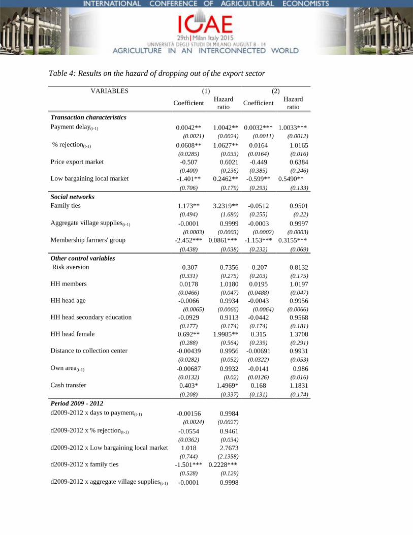
Table 4: Results on the hazard of dropping out of the export sector

VARIABLES (1) (2)

Coefficient Hazard

ratio Coefficient

Hazard

ratio

Transaction characteristics

Payment delay(t-1) 0.0042** 1.0042** 0.0032*** 1.0033***

(0.0021) (0.0024) (0.0011) (0.0012)

% rejection(t-1) 0.0608** 1.0627** 0.0164 1.0165

(0.0285) (0.033) (0.0164) (0.016)

Price export market -0.507 0.6021 -0.449 0.6384

(0.400) (0.236) (0.385) (0.246)

Low bargaining local market -1.401** 0.2462** -0.599** 0.5490**

(0.706) (0.179) (0.293) (0.133)

Social networks

Family ties 1.173** 3.2319** -0.0512 0.9501

(0.494) (1.680) (0.255) (0.22)

Aggregate village supplies(t-1) -0.0001 0.9999 -0.0003 0.9997

(0.0003) (0.0003) (0.0002) (0.0003)

Membership farmers' group -2.452*** 0.0861*** -1.153*** 0.3155***

(0.438) (0.038) (0.232) (0.069)

Other control variables

Risk aversion -0.307 0.7356 -0.207 0.8132

(0.331) (0.275) (0.203) (0.175)

HH members 0.0178 1.0180 0.0195 1.0197

(0.0466) (0.047) (0.0488) (0.047)

HH head age -0.0066 0.9934 -0.0043 0.9956

(0.0065) (0.0066) (0.0064) (0.0066)

HH head secondary education -0.0929 0.9113 -0.0442 0.9568

(0.177) (0.174) (0.174) (0.181)

HH head female 0.692** 1.9985** 0.315 1.3708

(0.288) (0.564) (0.239) (0.291)

Distance to collection center -0.00439 0.9956 -0.00691 0.9931

(0.0282) (0.052) (0.0322) (0.053)

Own area(t-1) -0.00687 0.9932 -0.0141 0.986

(0.0132) (0.02) (0.0126) (0.016)

Cash transfer 0.403* 1.4969* 0.168 1.1831

(0.208) (0.337) (0.131) (0.174)

Period 2009 - 2012

d2009-2012 x days to payment(t-1) -0.00156 0.9984

(0.0024) (0.0027)

d2009-2012 x % rejection(t-1) -0.0554 0.9461

(0.0362) (0.034)

d2009-2012 x Low bargaining local market 1.018 2.7673

(0.744) (2.1358)

d2009-2012 x family ties -1.501*** 0.2228***

(0.528) (0.129)

d2009-2012 x aggregate village supplies(t-1) -0.0001 0.9998

(0.0002) (0.0003)

d2009-2012 x membership farmers' group 1.787*** 5.9721***

(0.495) (3.019)

d2009-2012 x Risk aversion 0.111 1.1176

(0.411) (0.5069)

d2009-2012 x HH head female -0.822** 0.4395**

(0.419) (0.191)

d2009-2012 x own area(t-1) -0.0181 0.9821

(0.0259) (0.031)

d2009-2012 x Cash transfer -0.392 0.6756

(0.262) (0.185)

θ 1.03 e-7 1.03 e-7

Observations 1538

1538

Number of groups 278 278

Log-likelihood -1174.67 -1188.75

Standard errors in parenthesis: *** p<0.01, ** p<0.05, * p<0.1

Dummies for years and villages included.

Likelihood-ratio test of θ: p=0.498 for both models.

11. Appendix

Table A1. Explanation of variables

Variable Specification

% rejection Percentage of produce rejected by the exporter; calculated

as kg rejected/kg delivered*100

Aggregate village supplies Total sum of broccoli supplies delivered to the collection

center by village members; measured in metric tons

Broccoli area Total land area cultivated with broccoli in 2012, in solar

Broccoli income local market Income from broccoli sold in the local market in USD for

2012

Broccoli income total Total income from broccoli in USD for 2012 (calculated

based on survey data)

Cash transfer 1 if household is eligible for government cash transfer

program targeting poor households

Collection center only 1 if farmer sold broccoli exclusively to the collection

center in 2012

Distance to collection center Distance to the collection center in km

Distance to local market Distance to the nearest local market in km

Family ties 1 if family member works at the collection center

Farming experience Number of years the household has grown broccoli

HH head age Age of the household head in years

HH head female 1 if household head is female

HH head secondary education 1 if household head has obtained secondary education

HH member off-farm 1 if household head has off-farm employment

HH members Number of household members

Kg delivered Quantity of broccoli delivered to the export market in kg

Kg rejected Quantity rejected by the exporter in kg

Low bargaining local market 1 if average price obtained in the local market is lower

than export market price in 2012

Membership farmers' group 1 if household is a member of the farmers' group

Own area Total land area owned by the household in 2012, in solar

Payment delay Number of days after delivery until payment was received

(in 2012)

Price export market Price per kilogram paid by the exporter to the collection

center in USD

Relatives in export market Number of relatives delivering broccoli to the export

market

Relatives in local market Number of relatives delivering broccoli to the local market

Risk aversion

Partial risk aversion coefficient calculated according to

Binswanger (1980); normalized to a scale from 0 (low risk

aversion) to 1 (high risk aversion)

Total area

Total land area cultivated by the household in 2012

(owned, rented, and under sharecropping), in solar

Total farm income Total farm income in 2012 in USD

Total income

Total household income in 2012 in USD (incl. farm

income, off-farm income, remittances, cash transfers,

rents)

Total years of participation Number of years household has participated in the export

market

Note: Land area is measured in solar: 1 solar = approx. 1700m2

Table A2. Descriptive statistics for export market transaction variables per year

Year Variable Obs Mean

Std.

Dev. Min Max

2002

Kg delivered 112 5996.5 6056.514 127 30543

Kg rejected 112 514.4375 471.3525 4 2511

% rejection 112 0.095804 0.037142 0.02 0.2

Days to payment 111 47.04505 13.62577 17 96

2003

Kg delivered 166 8587.723 7437.829 280 34066

Kg rejected 166 594.5964 497.4679 11 2587

% rejection 166 0.073133 0.02071 0.03 0.14

Days to payment 166 27.21687 14.34345 6 101

2004

Kg delivered 164 9057.701 8087.636 160 34672

Kg rejected 164 334.3841 328.599 2 1454

% rejection 164 0.037744 0.028096 0.01 0.28

Days to payment 164 68.52439 14.35759 23 153

2005

Kg delivered 168 9607.327 8490.575 203 34500

Kg rejected 167 409.6048 376.4703 8 1724

% rejection 168 0.042619 0.013939 0 0.14

Days to payment 168 74.79762 12.74323 21 148

2006

Kg delivered 150 9049.487 7728.636 284 34109

Kg rejected 150 638.5467 608.9711 15 3064

% rejection 150 0.064867 0.024184 0.03 0.18

Days to payment 148 68.53378 11.45082 37 115

2007 Kg delivered 171 10736.37 7757.177 432 34947

Kg rejected 171 801.0058 1601.17 11 20261

% rejection 171 0.070175 0.043811 0.03 0.43

Days to payment 168 80.32143 34.4238 34 489

2008

Kg delivered 176 10588.84 8275.709 478 35275

Kg rejected 176 1773.614 1932.781 21 11507

% rejection 176 0.06125 0.021478 0.02 0.17

Days to payment 176 144.8636 24.67396 66 236

2009

Kg delivered 154 6019.455 5909.05 191 28781

Kg rejected 152 406.9934 430.0803 11 2673

% rejection 153 0.066994 0.032969 0.03 0.22

Days to payment 120 200.575 94.74634 0 388

2010

Kg delivered 146 4495.548 3892.135 111 19194

Kg rejected 146 389.2877 358.2424 10 1797

% rejection 146 0.089795 0.044029 0.03 0.42

Days to payment 145 49.62069 41.68184 0 367

2011

Kg delivered 132 4799.97 4512.431 152 23891

Kg rejected 132 592.7121 539.3078 27 2794

% rejection 132 0.133182 0.062362 0.05 0.55

Days to payment 132 52.34848 35.7472 0 217

2012

Kg delivered 88 1999.545 1881.352 119 10232

Kg rejected 88 229.8636 230.6466 6 1223

% rejection 88 0.115 0.046312 0.01 0.23

Days to payment 85 38.54118 26.77354 0 155 Note: Calculations based on data obtained from the collection center's records. Only the households included in the household

survey were used for calculating these values.

Table A3. Heckman model estimates of initial export market participation and extent of

participation

Variable

Probability of ever

supplying export

market

Quantity delivered

to export market in

first year (kg)

Distance to collection center -0.110***

(0.0132)

Family ties -0.0379 954.7

(0.813) (1,748)

Aggregate village supplies -0.000141 0.650

(0.0002) (0.700)

Risk aversion -0.0261 291.7

(0.307) (948.6)

HH members -0.183** 97.55

(0.0724) (163.0)

HH head secondary education -0.182 306.5

(0.272) (807.1)

HH head female -0.574* -1,802**

(0.347) (771.6)

Own area 0.0162** 163.3**

(0.00744) (79.12)

Cash transfer 0.106 -643.8

(0.256) (623.3)

Membership farmers' group 7.260*** 2,655***

(0.837) (819.0)

Price export market 2.281*** 163.4***

(0.292) (43.56)

Rho

-0.0151

(0.071)

Constant -41.15***

(5.341)

Observations 401 401 Robust standard errors in parentheses *** p<0.01, ** p<0.05, * p<0.1

Wald test for rho: p=0.1816

In the first stage probit model on the decision to ever participate in the export sector, we use the

distance to the collection center as exclusion restriction. The coefficient is statistically

significant, indicating that farmers located further away from the collection center are less likely

to participate in the export chain. Furthermore, female-headed households and larger households

(family size) have a lower probability to enter the export sector. On the other hand, land size

(owned area), membership in farmers' group and export market price positively influence the

decision to participate in the export market. The parameter 𝜌 is not statistically significant

indicating that there is no systematic unobserved differences between export sector participants

and non-participants.

Table A4. Fisher-type unit root test for panel data

Ho: All panels contain unit roots Number of panels = 283

Ha: At least one panel is stationary Avg. number of periods = 5.75

AR parameter: Panel-specific Asymptotics: T -> Infinity

Statistic p-value

Kg delivered

Inverse chi-squared(128) 205.3834 0

Inverse normal -5.3951 0

Inverse logit t(324) -5.1144 0

Modified inv. chi-squared 4.8365 0

Kg rejected

Inverse chi-squared(126) 261.311 0

Inverse normal -8.0771 0

Inverse logit t(319) -7.7579 0

Modified inv. chi-squared 8.5238 0

Payment delay

Inverse chi-squared(128) 182.1162 0.0012

Inverse normal -4.1785 0

Inverse logit t(324) -3.8992 0.0001

Modified inv. chi-squared 3.3823 0.0004

Table A5. Sargan/Hansen test

Sargan test of overid. restrictions Prob> chi2 = 0.415

(Not robust, but not weakened by many

instruments)

Hansen test of overid. restrictions Prob> chi2 = 0.164

(Robust, but weakened by many instruments.)

Difference in Hansen tests of exogeneity of instruments subsets

gmm(kg delivered(t-1), collapse lag(2 7))

Hansen test excluding group:

Prob > chi2 = 0.444

Difference (null H = exogenous): Prob > chi2 = 0.130

gmm(aggregate village supplies(t-1),

collapse lag(7 10))

Hansen test excluding group:

Prob > chi2 = 0.695

Difference (null H = exogenous): Prob > chi2 = 0.041

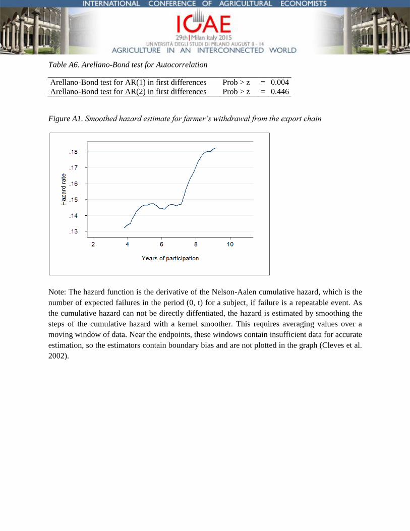
Table A6. Arellano-Bond test for Autocorrelation

Arellano-Bond test for AR(1) in first differences Prob > z = 0.004

Arellano-Bond test for AR(2) in first differences Prob > z = 0.446

Figure A1. Smoothed hazard estimate for farmer’s withdrawal from the export chain

Note: The hazard function is the derivative of the Nelson-Aalen cumulative hazard, which is the

number of expected failures in the period (0, t) for a subject, if failure is a repeatable event. As

the cumulative hazard can not be directly diffentiated, the hazard is estimated by smoothing the

steps of the cumulative hazard with a kernel smoother. This requires averaging values over a

moving window of data. Near the endpoints, these windows contain insufficient data for accurate

estimation, so the estimators contain boundary bias and are not plotted in the graph (Cleves et al.

2002).