Dynamics of Coupled Double Pendulums - TEAM … · Dynamics of Coupled Double Pendulums by ... The...
54
Transcript of Dynamics of Coupled Double Pendulums - TEAM … · Dynamics of Coupled Double Pendulums by ... The...

Technical University of Lodz
International Faculty of Engineering
Katedra Dynamiki Maszyn
Master of Science Thesis
Dynamics of Coupled Double
Pendulums
by
Mateusz Kubacki
Supervisor: Prof. dr hab. in». Tomasz Kapitaniak
�ód¹, 2011

Contents
1 Introduction 1
1.1 Aim of the thesis . . . . . . . . . . . . . . . . . . . . . . . . . . . . . 21.2 De�nitions . . . . . . . . . . . . . . . . . . . . . . . . . . . . . . . . 21.3 Methods of analysis of the system's dynamics . . . . . . . . . . . . . . 11
2 Creation of Model 12
2.1 Examined system: two double pendulums coupled by a sti� beam . . . 122.2 Derivation of the model . . . . . . . . . . . . . . . . . . . . . . . . . 13
3 Numerical Analysis 19
3.1 Simulation . . . . . . . . . . . . . . . . . . . . . . . . . . . . . . . . 193.2 Diagrams and analysis . . . . . . . . . . . . . . . . . . . . . . . . . . 21
4 Conclusions 46
Bibliography 47
List of Figures 49
i


Chapter 1
Introduction
The word pendulum comes form a Latin word pendulus which means "hanging". Thependulum has played great role in development of Western science and culture. Firstscienti�c observations of pendulum are often associated with Galileo Galilei (1554-1642). According to the story told (being perhaps apocryphal) Galileo observed themotion of swinging chandeliers in the cathedral of Pisa and using his heartbeat as atime measure noticed that even though the amplitude was diminishing the time of eachswing was consistent[2]. Since that times the scienti�c observations of pendulum andits application in mechanisms, such as clocks or metronome (the example of reversedpendulum), progressed.
Although a single pendulum seems like a simple system a set of pendulums canexhibit very complex behaviour. A double pendulum is an example of such a system,being in its nature a simple dynamical system but also being capable of exhibitingcomplex behaviour, including chaos.
With a set of two or more pendulums a phenomena of synchronization can beobserved. A word synchronization comes from a greek root sunkhronos that means"to share a common time". Historically the analysis of synchronization within thedynamical systems area has been studied since the earlier days of physics. It startedin 17th century with the �nding of Huygens that two pendulum clocks, coupled byhanging on the same beam become synchronised in phase.[4] He originally thought thatthe synchronization occurs due to air currents shared by both pendulums, but laterafter several tests attributed the occurrence of the phenomena to the imperceptiblemotion of the beam from which both of the pendulum clocks were suspended.[3]Recently, the search of synchronization has moved to chaotic systems. In order toperform the analysis, the model of the system must be derived.
Achievements of Lagrange and Hamilton among the others make it possible toconstruct very complicated models describing behaviour of di�erent mechanical devicesor physical phenomena. The models then can be calculated, often numerically allowingto test the systems without need to build the physical model and risk its damage incase of failures.
1

1.1 Aim of the thesis
The aim of the thesis is to investigate the process of synchronization of two doublependulums coupled through elastic structure. The analysis of the behaviour of theconsidered system is performed basing on the bifurcation diagrams, phase portraitsand Poincar'e maps. Numerical calculations are performed by written beforehandC++ program. Equations of the system motion is derived by mean of the Lagrangemethod. The purpose of the analysis is to the system's behaviour for di�erent fre-quency and amplitude of the excitation. Finally, the in�uence of parameters changeson synchronization of the pendulums is investigated.
1.2 De�nitions
In this section de�nitions of terms used in this thesis will be presented.
De�nition 1. Considering a following set of di�erential equations
dx
dt= f(x), x(t0) = x0, (1.1)
where vector functionf : D → Rn,
is continuos with respect to time t and variable x, D is an open subset Rn+1, x ∈Rn, t ∈ R. Equation set 1.1 is called n-dimensional autonomous set of equa-
tions, because time does not occur explicitly on the right hand side of equations.Similarly the set of equations
dx
dt= f(x, t), x(t0) = x0, (1.2)
in which time occurs explicitly on the right hand side of the equations, is calledn-dimensional autonomous set of equations. The subset D is called a phasespace. If there exists T>0 such, that
f(x, t) = f(x, t = T )
for every x and to, then the set of equations 1.2 is called periodic with a periodof T [5].
De�nition 2. A dynamical system described by set of equations 1.1 is themapping
Φ : R×D → Rn,
de�ned by solution x(t) of the set of equations 1.1 [5].
De�nition 3. A function f representing the right hand side of the set of equations1.1 de�nes the mapping f
f : D → Rn,
de�ning the vector �eld in Rn In order to show the dependancy of solution of setof equations 1.1 on the initial condition in an explicit way, the solution is oftenwritten in the form Φt(x0) [5].
2

De�nition 4. The mapping
Φt : D → Rn
is called the phase �ow [5].
De�nition 5. Consider the autonomous case of the equation 1.1 written in thefollowing form
dx1
dt= fi(x), i = 1, 2, ..., n.
If f1(x) 6= 0, then the x1 component of the vector x can be taken as a new inde-pendent variable. The following set of equations will be obtained
dx2
dx1
=f2(x)
f1(x)
...
dxndx1
=fn(x)
f1(x)
(1.3)
The solution of the equations 1.3 in a phase space is called the trajectory (anorbit) of a system.[5]
De�nition 6. A minimal subset A in phase space of an equation f : Rn × R →Rn, t ∈ R, which is reachable asymptotically by the trajectory x(t), when t →∞(t → −∞), is called an attractor (negative attractor). The concept of at-tractor is shown on the Figure 1.1. For every attractor A there exists subset b(A),such that for ever x0 ∈ b(A) the phase trajectory x(t) that begins in x0 tends to Awhen t → ∞. Subset b(A) is called the basin of attraction of attractor A. Fornegative attractor b(A) has the aforementioned property for t→ −∞. [5]
Figure 1.1: Attractor A and its basin of attraction b(A)
De�nition 7. The subset A is called asymptotically stable attractor, if for everysu�ciently small neighbourhood U(A) exist such neighbourhood V (A), that forevery x0 ∈ U(A), the phase trajectory x(t) thet begins in x0 stays in V (A) forevery t, and the distance of the point x(t) from the attractor A tends to zero fort→∞. The de�nition of asymptotical stability of the attractor A shows, that thebasin of attraction of such attractor contains its neighbourhood. The di�erencebetween stable and statically stable attractor shows the picture 1.2. [5]
3

Figure 1.2: Attractors: a) stable; b) asymptotically stable
De�nition 8. In a general case let x = Φ(t) be the solution of the system 1.1 andlet there be such constant T , that
Φ(t) = Φ(t+ T )
for every t, then Φ(t) is called the periodical solution of a period T . The closedcurve in the phase space corresponds to the periodical solution, and such closedphase trajectory implies the periodical solution. [5]
De�nition 9. The periodical solution of the autonomous system 1.1, that areattractors or negative attractors, are called also limit cycles. If a limit cycle isavailable through the solution when t → ∞, then it is statical and an attractor.If the limit cycle has this property for t → −∞, then it is unstable and is anunstable, negative attractor. [5]
De�nition 10. Iterations of the map mapping given interval on the same intervalare the simplest examples of nonlinear, dissipative dynamical systems. Iterationsof a form
xn → xn+1 = f(xn), (1.4)
where f : [−1, 1] → [−1, 1], n = 1, 2, ..., and x0 is given throughout the initialcondition x0 can be treated as discrete time equivalent of dynamical systems withcontinuous time. In mapping 1.4 - n corresponds to the variable describing time[5].
Figure 1.3: Poincaré map construction
4
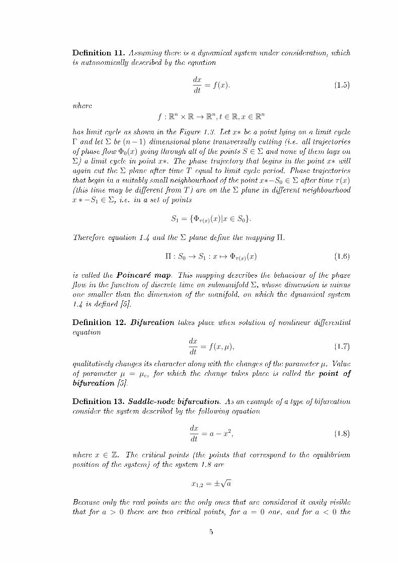
De�nition 11. Assuming there is a dynamical system under consideration, whichis autonomically described by the equation
dx
dt= f(x). (1.5)
where
f : Rn × R→ Rn, t ∈ R, x ∈ Rn
has limit cycle as shown in the Figure 1.3. Let x∗ be a point lying on a limit cycleΓ and let Σ be (n−1)-dimensional plane transversally cutting (i.e. all trajectoriesof phase �ow Φ0(x) going through all of the points S ∈ Σ and none of them lays onΣ) a limit cycle in point x∗. The phase trajectory that begins in the point x∗ willagain cut the Σ plane after time T equal to limit cycle period. Phase trajectoriesthat begin in a suitably small neighbourhood of the point x∗−S0 ∈ Σ after time τ(x)(this time may be di�erent from T ) are on the Σ plane in di�erent neighbourhoodx ∗ −S1 ∈ Σ, i.e. in a set of points
S1 = {Φτ(x)(x)|x ∈ S0}.
Therefore equation 1.4 and the Σ plane de�ne the mapping Π,
Π : S0 → S1 : x 7→ Φτ(x)(x) (1.6)
is called the Poincaré map. This mapping describes the behaviour of the phase�ow in the function of discrete time on submanifold Σ, whose dimension is minusone smaller than the dimension of the manifold, on which the dynamical system1.4 is de�ned [5].
De�nition 12. Bifurcation takes place when solution of nonlinear di�erentialequation
dx
dt= f(x, µ), (1.7)
qualitatively changes its character along with the changes of the parameter µ. Valueof parameter µ = µc, for which the change takes place is called the point of
bifurcation [5].
De�nition 13. Saddle-node bifurcation. As an example of a type of bifurcationconsider the system described by the following equation
dx
dt= a− x2, (1.8)
where x ∈ Z. The critical points (the points that correspond to the equilibriumposition of the system) of the system 1.8 are
x1,2 = ±√a
Because only the real points are the only ones that are considered it easily visiblethat for a > 0 there are two critical points, for a = 0 one, and for a < 0 the
5

equation 1.8 has no critical points. The equation 1.8 can be analytically integratedcan by presented in a form
x(t) =
√ax0 +
√a tanh(
√at)√
a+ x0 tanh(√at)
,
x0
1 + x0t,
√−ax0 −
√−a tanh(
√−at)√
−a+ x0 tanh(√−at)
,
for a > 0
for a = 0
for a < 0
(1.9)
In the equation 1.9 x0 = x(0) is the initial condition. Analysing the course of thevariability of the function of solution of x(t) it can be noticed, that
limt→∞
x(t) =√a, when: a > 0, x0 > −
√a
limt→∞
x(t) = −√a, when: a > 0, x0 < −
√a
limt→∞
x(t) = 0, when: a = 0, x0 > 0,
andlimt→ 1
x0
x(t) = −∞, when: a = 0, x0 < 0
limt→√a arctanh
−√
ax0
x(t) = −∞, when: a > 0, x0 < −√a
limt→√−a arctanh
−√−a
x0
x(t) =∞, when: a > 0, x0 < 0.
The properties of the solution 1.9 are presented on the Figure 1.4 From the above
Figure 1.4: Saddle-node bifurcation
analysis it results, that the number of critical points changes, when the value ofparameter a goes through 0, and that the stability of the critical points changes,when x = ±
√a goes through zero. This type of bifurcation is called the saddle-
node bifurcation. [5]
6

De�nition 14. The Hopf bifurcation occurs when a critical point loses its sta-bility, resulting in occurrence of periodic solution (limit cycle). Such bifurcationcan be explained by an exemplary set of di�erential equations
dx
dt= −y + (a− x2 − y2)x
dy
dt= x+ (a− x2 − y2)y
(1.10)
where a ∈ R. Assumingdx
dt=dy
dt= 0
it can be shown, that (x, y) = (0, 0) is the critical point. By linearisation of theequation 1.10 in the neighbourhood of the critical point gives
dx
dt= −y + ax
dy
dt= x+ ay
(1.11)
The solution of linearised system 1.11 is the linear combination of the functions
x(t) = eλtu
y(t) = eλtv,
that ful�l the equationAu = su,
where s is an eigenvalue, u = [u, v]T are eigenvectors, and A is a matrix of theform
A =
[a −11 a
].
Therefore
0 = det(A− sI) =
∣∣∣∣ a− s −11 a− s
∣∣∣∣ = (a− s)2 + 1, (1.12)
THe solution x = y = 0 of the linearised system is stable, when
Re(s1,2) < 0,
i.e. when a < 0, and unstable when a > 0. The form of set of equations 1.10was chosen in such a way, so that it is possible to obtain an analytical solution.Introducing polar coordinates x = r cos Θ, y = r sin Θ for r > 0 it can be easilyshown, that x+ iy = r exp iΘ. Multiplying second one of equations 1.10 by i, andsubsequently adding it to the �rst equation, the following formula is obtained
d(reiΘ)
dt=dx
dt+ i
dy
dt= −y + ix+ (a− x2 − y2)(x+ iy) (1.13)
or (dr
dt+ ir
dΘ
dt
)eiΘ = ireiΘ + (a− r2)reiΘ.
7

Dividing both sides of this equation by exp(iΘ) and comparing the real and imag-inary parts on both sides of the equation the yields
dr
dt= r(a− r2)
dΘ
dt= 1
(1.14)
Hence
r2(t) =
ar02
r02+(a−r02)e−2at
r02
1+2r02t
a 6= 0
a = 0,(1.15)
and
Θ = t+ Θ0, r0 = r(0), Θ0 = Θ(0).
The solution 1.15 can be presented in a form of phase trajectory
x = (x(t), y(t))
on a plane, assuming the Cartesian coordinate system. For a 6 0, all phasetrajectories x(t) → 0, when t → ∞ and the point x(0, 0) is the attractor. Thebehaviour of the trajectories in this case is shown on the Figure 1.5 However for
Figure 1.5: The behaviour of the phase trajectories before Hopf bifurcation
a > 0 point x(0, 0) becomes a negative attractor and new stable solution being alimit cycle appears
x =√a cos(t+ Θ0)
y =√a sin(t+ Θ0)
Such solution is shown on the Figure 1.6 All phase trajectories that begin in anarbitrary point of the phase space other than x(0, 0) tend to the periodic trajectory,in this case described by
x2 + y2 = a.
Described Hopf bifurcation is the supercritical bifurcation, i.e. stable limit cyclesubstitutes stable critical point, when a goes through 0. In case of this bifurcationthe real part of the couple of complex eigenvalues λ1,2 changes the sign from minusto plus, when a goes through the critical value a0 and as a result the critical pointbecomes substituted by the limit cycle, as shown on the Figure 1.7.[5]
8

Figure 1.6: The behaviour of the phase trajectories after Hopf bifurcation
Figure 1.7: Limit cycle created as a result of Hopf bifurcation
De�nition 15. Neimark-Sacker bifurcation is the birth of a closed invariantcurve from a �xed point in dynamical systems with discrete time (iterated maps),when the �xed point changes stability via a pair of complex eigenvalues with unitmodulus.
Consider a mapx 7→ f(x, α), x ∈ Rn (1.16)
depending on the parameter α ∈ R, where f is smooth. Suppose that for allsu�ciently small |α| the system has a family of �xed points x0(α). Further Assumethat it's Jacobian matrix A(α) = fx(x
0(α), α) has one pair of complex eigenvaluesλ1,2(α) = r(α)e±iθ(α) on the unit circle when α = 0, i.e., r(0) = 1 and 0 <θ(0) < π. Then, generically as α passes through α = 0, the �xed point changesstability and a unique closed invariant curve bifurcates from it. This bifurcationis characterized by a single bifurcation condition |λ1,2| = 1 (has codimension one)and appears generically in one-parameter families of smooth maps.
De�nition 16. Synchronization of chaos refers to the process where two (ormore) chaotic systems, which are either equivalent or non-equivalent, adjust agiven property of their motion to a common behaviour due to coupling or a ex-citation (periodical or noisy). There are many di�erent synchronization statesdistinguished [4].
De�nition 17. Complete synchronization [4] is the perfect hooking of thetrajectories of two systems, achieved by means of a coupling signal, in sauch a
9

way that they remain in step with each other in the course of time. Assumingthat two systems are represented by phase trajectories x(t) and y(t), the completesynchronization takes place if the following relation is true for all t > 0:
limt→∞|x(t)− y(t)| = 0. (1.17)
De�nition 18. Phase synchronization [4] is reached when a locking of phaseis produced, when correlation of amplitudes remain weak. By the de�nition phasesynchronization takes place when two systems represented by the phases ϕ1,2 withratio n : m (n and m are integers) of two systems are locked, which means that
|nϕ1 −mϕ2| < const. (1.18)
As a result of phase synchronization, the frequencies ωi = ϕi are also locked, i.e.
nω1 −mω2 = 0.
10

1.3 Methods of analysis of the system's dynamics
There is a number of methods that can be useful when it comes to analysis of thedynamics systems. The ones employed to analysis of this systems are:
• Phase portrait
• Poincaré Map
• Bifurcation Diagram
Phase portrait is simply a projection of phase trajectory (de�nition 5) on thephase plane. The shape of the phase portrait gives information about system be-haviour. The closed loop shape of the phase portrait indicates the periodic behaviourof the system whereas non regular open shape may suggest chaotic behaviour.
Poincaré map, as de�ned previously (see de�nition 11), supplies informationhelpful in recognising whether the behaviour of the system under consideration isperiodic, quasiperiodic or (hyper)chaotic. The single point plotted on a map impliesperiodic behaviour. If the map presents a closed loop shape, the system's behaviouris quasiperiodic. Chaotic behaviour may be suggested by a fractal structure created inthe plot, hyperchaotic behaviour is indicated by irregular points.
Bifurcation diagram can be described as a collection of Poincaré maps for chang-ing bifurcation (or control) parameter. The Poincaré maps are projected on a x − ycoordinate system, where x-axis corresponds to the values of the control parameterand on y-axis is a selected variable which describes the system. The analysis of thebifurcation diagram is analogical as for Poincaré maps. Single point for a given controlparameter value means that the behaviour is periodic. A collection of points distributedregularly implies quasiperiodic behaviour whereas an irregularly distributed collectionof points can suggest (hyper)chaos.
11
Chapter 2
Creation of Model
2.1 Examined system: two double pendulums cou-
pled by a sti� beam
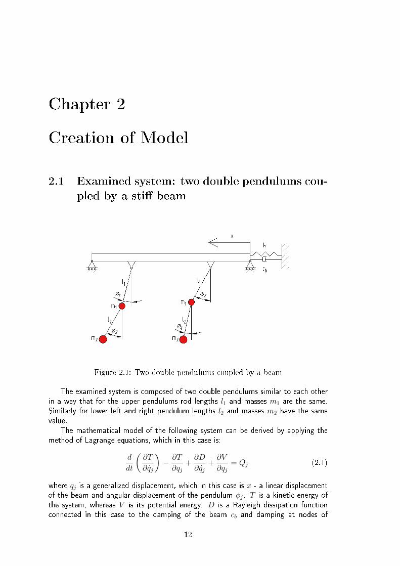
Figure 2.1: Two double pendulums coupled by a beam
The examined system is composed of two double pendulums similar to each otherin a way that for the upper pendulums rod lengths l1 and masses m1 are the same.Similarly for lower left and right pendulum lengths l2 and masses m2 have the samevalue.
The mathematical model of the following system can be derived by applying themethod of Lagrange equations, which in this case is:
d
dt
(∂T
∂qj
)− ∂T
∂qj+∂D
∂qj+∂V
∂qj= Qj (2.1)
where qj is a generalized displacement, which in this case is x - a linear displacementof the beam and angular displacement of the pendulum φj. T is a kinetic energy ofthe system, whereas V is its potential energy. D is a Rayleigh dissipation functionconnected in this case to the damping of the beam cb and damping at nodes of
12
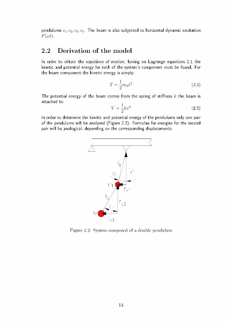
pendulums c1, c2, c3, c4. The beam is also subjected to horizontal dynamic excitationF (ωt).
2.2 Derivation of the model
In order to obtain the equations of motion, basing on Lagrange equations 2.1 thekinetic and potential energy for each of the system's component must be found. Forthe beam component the kinetic energy is simply:
T =1
2m3x
2 (2.2)
The potential energy of the beam comes from the spring of sti�ness k the beam isattached to:
V =1
2kx2 (2.3)
In order to determine the kinetic and potential energy of the pendulums only one pairof the pendulums will be analysed (Figure 2.2). Formulae for energies for the secondpair will be analogical, depending on the corresponding displacements.
Figure 2.2: System composed of a double pendulum
13

Analysing the �rst pendulum, the general formula of kinetic energy is:
T =1
2mr2 (2.4)
where r is a displacement. In case of the pendulum, the displacement can bedecomposed into two displacement vectors, horizontal rjx and vertical rjy. In thiscase, because
rj =√rjx2 + rjy2
and
rj =√r2jx + r2
jy
the equation 2.4 takes the following form:
Tj =1
2mj(r
2jx + r2
jy) (2.5)
In case of the upper pendulum, resulting from the trigonometric dependancies, andalso taking into consideration a horizontal displacement x of a beam the pendulum isattached to:
r1x = x+ l1 sinφ1 (2.6)
r1y = l1 cosφ1 (2.7)
The displacement components for lower pendulum have to be taken in respect topoint of attachment of the �rst pendulum, hence the r1x and r2y have to be addedrespectively:
r3x = r1x + l2 sinφ3
r3y = r1y + l2 cosφ3
After substitution the equations take the following form:
r3x = x+ l1 sinφ1 + l2 sinφ3 (2.8)
r3y = l1 cosφ1 + l2 cosφ3 (2.9)
After di�erentiation the velocity components for those pendulums can be obtained:
r1x = x+ l1φ1 cosφ1
r1y = −l1φ1 sinφ1
r3x = x+ l1φ1 cosφ1 + l2φ3 cosφ3
r3y = −l1φ1 sinφ1 − l2φ3 sinφ3
(2.10)
For the second pair of pendulums the velocity components have analogical form, onlywith corresponding angles φ2 and φ4 instead of φ1 and φ3.
Since the kinetic energy of the system is equal to sum of kinetic energies of indi-vidual components, the kinetic energy of this system has the following form:
T =1
2
[m1
(r2
1x + r21y + r2
2x + r22y
)+m2
(r2
3x + r23y + r2
4x + r24y
)+m3x
](2.11)
After substituting velocity components of pendulums into equation 2.11 the fol-lowing formula is obtained:
T = 12m3x
2 +m1x2 +m1xl1φ1 cosφ1 + 1
2m1l
21φ
21 +m1xl1φ2 cos Φ2 + 1
2m1l
21φ
22+
+m2x2 +m2x
2l1φ1 cosφ1 +m2xl2φ3 cosφ3 + 12m2l
21φ
21 +m2l1l2φ1φ3 cos(φ1 − φ3)+
+12m2l
22φ
23 +m2xl1φ2 cosφ2 +m2xl2φ4 cosφ4 + 1
2m2l
21φ
22 +m2l1l2φ2φ4 cos(φ2 − φ2)+
+12m2l2φ4
(2.12)
14

Figure 2.3: System composed of two pendulums - potential energy
Next step is �nding the potential energy for pendulums and the beam. In case ofthe beam it is a potential energy of the spring, which is equal to
Vb =1
2kx2
As for the pendulums, one again only one pair will be considered for now and the energyfor the second pair will be derived by analogy. The potential energy for pendulumswill be derived from well known equation:
V = mgh
In case of upper pendulum, the height h1, as visible on Figure 2.3 is equal to:
h1 = l1 − l1 cosφ1
Hence the potential energy for the �rst pendulum is equal to:
V1 = m1gl1(1− cosφ1) (2.13)
Analogically, h3 of the second pendulum is equal to:
h3 = l2 − l2 cosφ3
Taking into consideration h1 the formula for potential energy is as follows:
V3 = m2g(l1 − l1 cosφ1 + l2 − l2 cosφ3) (2.14)
Analogically, for the second pair of pendulums:
V2 = m1gl1(1− cosφ2), (2.15)
V4 = m2g(l1 − l1 cosφ2 + l2 − l2 cosφ4) (2.16)
15

Hence, the total potential energy of the whole system is equal to:
V = m1gl1(1− cosφ1) +m2g(l1 − l1 cosφ1 + l2 − l2 cosφ3)++m1gl1(1− cosφ2) +m2g(l1 − l1 cosφ2 + l2 − l2 cosφ4) + 1
2kx2 (2.17)
Having the potential and kinetic energy calculated, in order to construct equations ofmotion according to the formula 2.1 a series of derivatives must be found. Namely,derivatives of potential energy over all of the displacements ∂V
∂qj, derivatives of kinetic
energy over all of the displacements ∂T∂qj
and velocities ∂T∂qj
as well as theirs derivatives
over time ddt
(∂T∂qj
)After di�erentiating kinetic energy with respect to all displacements
the following formulae are obtained:
∂T∂φ1
= −m1xl1φ1 sinφ1 −m2xl1φ1 sinφ1 −m2l1l2φ1φ3 sin (−φ3 + φ1) ,∂T∂φ2
= −m1xl1φ2 sinφ2 −m2xl1φ2 sinφ2 −m2l1l2φ2φ4 sin (−φ4 + φ2) ,∂T∂φ3
= −m2xl2φ3 sinφ3 +m2l1l2φ1φ3 sin(−φ3 + φ1),∂T∂φ4
= −m2xl2φ4 sinφ4 +m2l1l2φ2φ4 sin(−φ4 + φ2),∂T∂x
= 0
(2.18)
Then, after di�erentiation of kinetic energy with respect to the velocities and thenwith respect to time, the following formulae are obtained:
ddt
(∂T∂φ1
)= m1xl1 cosφ1 −m1xl1φ1 sinφ1 +m1l
21φ1+
+m2xl1 cosφ1 −m2xl1φ1 sinφ1 +m2l21φ1 +m2l1l2φ3 cos(−φ3 + φ1)+
+m2l1l2φ3(−φ3 + φ1) sin(−φ3 + φ1),ddt
(∂T∂φ2
)= m1xl1 cosφ2 −m1xl1φ1 sinφ2 +m1l
21φ2+
+m2xl1 cosφ2 −m2xl1φ2 sinφ1 +m2l21φ2 +m2l1l2φ4 cos(−φ4 + φ2)+
+m2l1l2φ4(−φ4 + φ2) sin(−φ4 + φ2),ddt
(∂T∂φ3
)= m2xl2 cosφ3 −m2xl2φ3 sinφ3 +m2l1l2φ1 cos(−φ3 + φ1)−
−m2l1l2φ1(−φ3 + φ1) sin(−φ3 + φ1) +m2l22φ3,
ddt
(∂T∂φ4
)= m2xl2 cosφ4 −m2xl2φ4 sinφ4 +m2l1l2φ2 cos(−φ4 + φ2)−
−m2l1l2φ2(−φ4 + φ2) sin(−φ4 + φ2) +m2l22φ4,
ddt
(∂T∂x
)= m3x+ 2m1x−m1l1φ
21 sinφ1 +m1l1φ1 cosφ1−
−m1l1φ22 sinφ2 +m1l1φ2 cosφ2 + 2m2x−m2l1φ
21 sinφ1+
+m2l1φ1 cosφ1 −m2l2φ23 sinφ3 +m2l2φ3 cosφ3 −m2l1φ
22 sinφ2+
+m2l1φ2 cosφ2 −m2l2φ24 sinφ4 +m2l2φ4 cosφ4
(2.19)
The derivatives of potential energy with respect to all the displacements are equal to:
∂V∂φ1
= m1gl1 sinφ1 +m2gl1 sinφ1,∂V∂φ2
= m1gl1 sinφ2 +m2gl1 sinφ2,∂V∂φ3
= m2gl2 sinφ3,∂V∂φ4
= m2gl2 sinφ4,∂V∂x
= kx
(2.20)
16
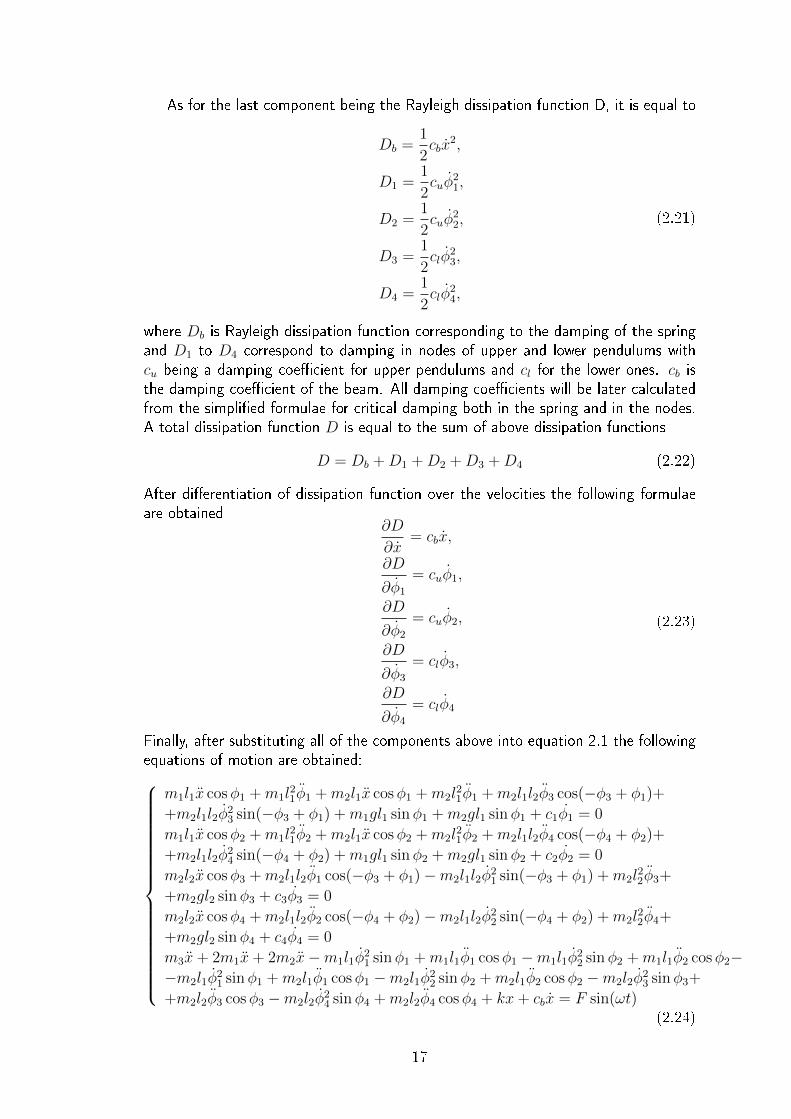
As for the last component being the Rayleigh dissipation function D, it is equal to
Db =1
2cbx
2,
D1 =1
2cuφ
21,
D2 =1
2cuφ
22,
D3 =1
2clφ
23,
D4 =1
2clφ
24,
(2.21)
where Db is Rayleigh dissipation function corresponding to the damping of the springand D1 to D4 correspond to damping in nodes of upper and lower pendulums withcu being a damping coe�cient for upper pendulums and cl for the lower ones. cb isthe damping coe�cient of the beam. All damping coe�cients will be later calculatedfrom the simpli�ed formulae for critical damping both in the spring and in the nodes.A total dissipation function D is equal to the sum of above dissipation functions
D = Db +D1 +D2 +D3 +D4 (2.22)
After di�erentiation of dissipation function over the velocities the following formulaeare obtained
∂D
∂x= cbx,
∂D
∂φ1
= cuφ1,
∂D
∂φ2
= cuφ2,
∂D
∂φ3
= clφ3,
∂D
∂φ4
= clφ4
(2.23)
Finally, after substituting all of the components above into equation 2.1 the followingequations of motion are obtained:
m1l1x cosφ1 +m1l21φ1 +m2l1x cosφ1 +m2l
21φ1 +m2l1l2φ3 cos(−φ3 + φ1)+
+m2l1l2φ23 sin(−φ3 + φ1) +m1gl1 sinφ1 +m2gl1 sinφ1 + c1φ1 = 0
m1l1x cosφ2 +m1l21φ2 +m2l1x cosφ2 +m2l
21φ2 +m2l1l2φ4 cos(−φ4 + φ2)+
+m2l1l2φ24 sin(−φ4 + φ2) +m1gl1 sinφ2 +m2gl1 sinφ2 + c2φ2 = 0
m2l2x cosφ3 +m2l1l2φ1 cos(−φ3 + φ1)−m2l1l2φ21 sin(−φ3 + φ1) +m2l
22φ3+
+m2gl2 sinφ3 + c3φ3 = 0
m2l2x cosφ4 +m2l1l2φ2 cos(−φ4 + φ2)−m2l1l2φ22 sin(−φ4 + φ2) +m2l
22φ4+
+m2gl2 sinφ4 + c4φ4 = 0
m3x+ 2m1x+ 2m2x−m1l1φ21 sinφ1 +m1l1φ1 cosφ1 −m1l1φ
22 sinφ2 +m1l1φ2 cosφ2−
−m2l1φ21 sinφ1 +m2l1φ1 cosφ1 −m2l1φ
22 sinφ2 +m2l1φ2 cosφ2 −m2l2φ
23 sinφ3+
+m2l2φ3 cosφ3 −m2l2φ24 sinφ4 +m2l2φ4 cosφ4 + kx+ cbx = F sin(ωt)
(2.24)
17

Before the equations can be inserted into program however, all of the components ofacceleration have to go on the left side of equations forming an inertia matrix, whileall the rest goes on the right side of equations:
x(m1l1 cosφ1 +m2l1 cosφ1) + φ1(m1l21 +m2l
21) +m2l1l2φ3 cos(−φ3 + φ1) =
= −m2l1l2φ23 sin(−φ3 + φ1)−m1gl1 sinφ1 −m2gl1 sinφ1 − c1φ1
x(m1l1 cosφ2 +m2l1 cosφ2) + φ2(m1l21 +m2l
21) +m2l1l2φ4 cos(−φ4 + φ2) =
= −m2l1l2φ24 sin(−φ4 + φ2)−m1gl1 sinφ2 −m2gl1 sinφ2 − c2φ2
m2l2x cosφ3 +m2l1l2φ1 cos(−φ3 + φ1) +m2l22φ3 = m2l1l2φ
21 sin(−φ3 + φ1)−
−m2gl2 sinφ3 − c3φ3
m2l2x cosφ4 +m2l1l2φ2 cos(−φ4 + φ2) +m2l22φ4 = m2l1l2φ
22 sin(−φ4 + φ2)−
−m2gl2 sinφ4 − c4φ4
(2m1 + 2m2 +m3)x+ φ1(m1l1 cosφ1 +m2l1 cosφ1) + φ2(m1l1 cosφ2 +m2l1 cosφ2)+
+m2l2φ3 cosφ3 +m2l2φ4 cosφ4 = F sin(ωt) +m1l1φ21 sinφ1 +m1l1φ
22 sinφ2+
m2l1φ21 sinφ1 +m2l1φ
22 sinφ2 +m2l2φ
23 sinφ3 +m2l2φ
24 sinφ4 − kx− cbφb
(2.25)Equations prepared in this form are ready to be put into the program which performsnumerical computations based on them.
18

Chapter 3
Numerical Analysis
In this the results of numerical computations based on the equations included in chapter2 will be presented. The program was written in C++ language and slightly modi�edto ful�l the needs of the task described. The program is designed to be run underMicrosoft Windows environment. The equations were brought down to the form visiblein equation 2.25 and the put into the program and subsequently solved using 4th orderRunge-Kutta method with �xed time step. The time step used for this simulation wasequal to T/3600 with T being the period of excitation. Three versions of the programswere in use as three di�erent diagram types were needed for the analysis - phaseportraits, Poincaré maps and bifurcation diagrams. As a result of the calculations theprogram produced text �les containing the parameters needed for the diagrams in aform ready to be imported into workbook based programs like MS Excel.
3.1 Simulation
The parameters of the system had to be chosen in a way that they are reasonable fromthe mechanical point of view. The parameters of the system chosen for the simulationwere as follows:
m1 = 1 [kg],m2 = 0.5 [kg],m3 = 3 [kg],l1 = 1.5 [m],l2 = 1 [m]
The system was analysed for four di�erent amplitudes of excitation: 200, 250, 300and 350 N. The coe�cient of sti�ness of the spring was assumed to be:
k = 850
[N
m
]
The damping coe�cients for the beam cb and at the nodes of upper c1,c2 and lowerc3,c4 pendulums are, as mentioned before, based on the values of critical dampingcoe�cients and diminished by an appropriate factor:
19

cb = 0.3(√m3k)
[kg · Nm
],
c1 = 0.1(√gl1)
[m2
s2
],
c2 = 0.1(√gl1)
[m2
s2
],
c3 = 0.1(√gl2)
[m2
s2
],
c4 = 0.1(√gl2)
[m2
s2
].
The initial conditions for the simulation were as follows:
x = 0.1 [m],φ1 = π
6[rad],
φ2 = −π4[rad],
φ3 = π8[rad],
φ4 = −π4[rad].
The system was investigated for four di�erent values of excitation amplitude - 200 [N],250 [N], 300 [N], 350[N].
After the software calculations the text �les containing the results were importedinto a workbook in order to produce bifurcation diagrams, phase portraits and Poincarémaps (see chapter 1.3) helpful in analysis of the systems behaviour.
20

3.2 Diagrams and analysis
In order to analyse the synchronization of the pendulums it would be very convenientto introduce two new variables e1 and e2, such that
e1 = φ1(t)− φ2(t),e2 = φ3(t)− φ4(t)
(3.1)
Those variables de�ne the distance between conjugated trajectories of the subsystemsφ1(t) and φ2(t) for the �rst one and φ3(t) with φ4(t) for the second one in thephase plane. They will be later called the phase di�erences. Such variables make�nding a complete synchronization of pendulums easier as according to the de�nition17 the complete synchronization occurs when the phase di�erence is equal to zero.Instead of introducing those variables into Lagrange equations, they were calculated ina workbook based software by simply subtracting columns with results correspondingto φ1, φ2, φ3 and φ4 in order to obtain values of e1 and e2 respectively.
The anti-phase synchronization (with opposite phases for which the sums φ1 + φ2
or φ3 + φ4 would be equal to zero) was not observed at all for given range of controlparameter and initial conditions.
The areas on bifurcation diagrams for e1 and e2 (Figures 3.1 and 3.2) where valueof phase di�erence is equal to zero mean that system synchronises completely forthose values of control parameter. It is clearly visible that pendulums are in completesynchronization (upper and lower ones with respect to each other respectively) inmost part of the investigated ω range. It is so for all investigated values of excitationamplitude except for 350 [N] which corresponds to Figures 3.1.D and 3.2.D.
It can be noticed that along with the incrementation of the excitation amplitudethe range of ω values for which the complete synchronization does not occur increasesas well. It is also worth mentioning that the graphs for e1 = φ1 − φ2 and e2 =φ3 − φ4 are similar for respective excitation amplitude values. In all cases occurs lackof synchronization for ω equal to around 2.5 [Hz]. Also for excitation frequency higherthan 2.5 [Hz] the lack of synchronization of both upper and lower pendulums occursfor similar ω values for respective excitation amplitude F values.
The relationship between system's behaviour (periodic, quasiperiodic and chaotic)and pendulums synchronization will be later analysed. It will be very useful to de-termine wether the synchronization of pendulum or lack thereof corresponds to someparticular systems behaviour. This could be done by comparing bifurcation diagramsfor angular displacements of pendulums with ω taken as a control parameter withFigures 3.1 and 3.2. Also phase portraits will be useful to determine the nature ofsystem's behaviour for chosen control parameter values.
21
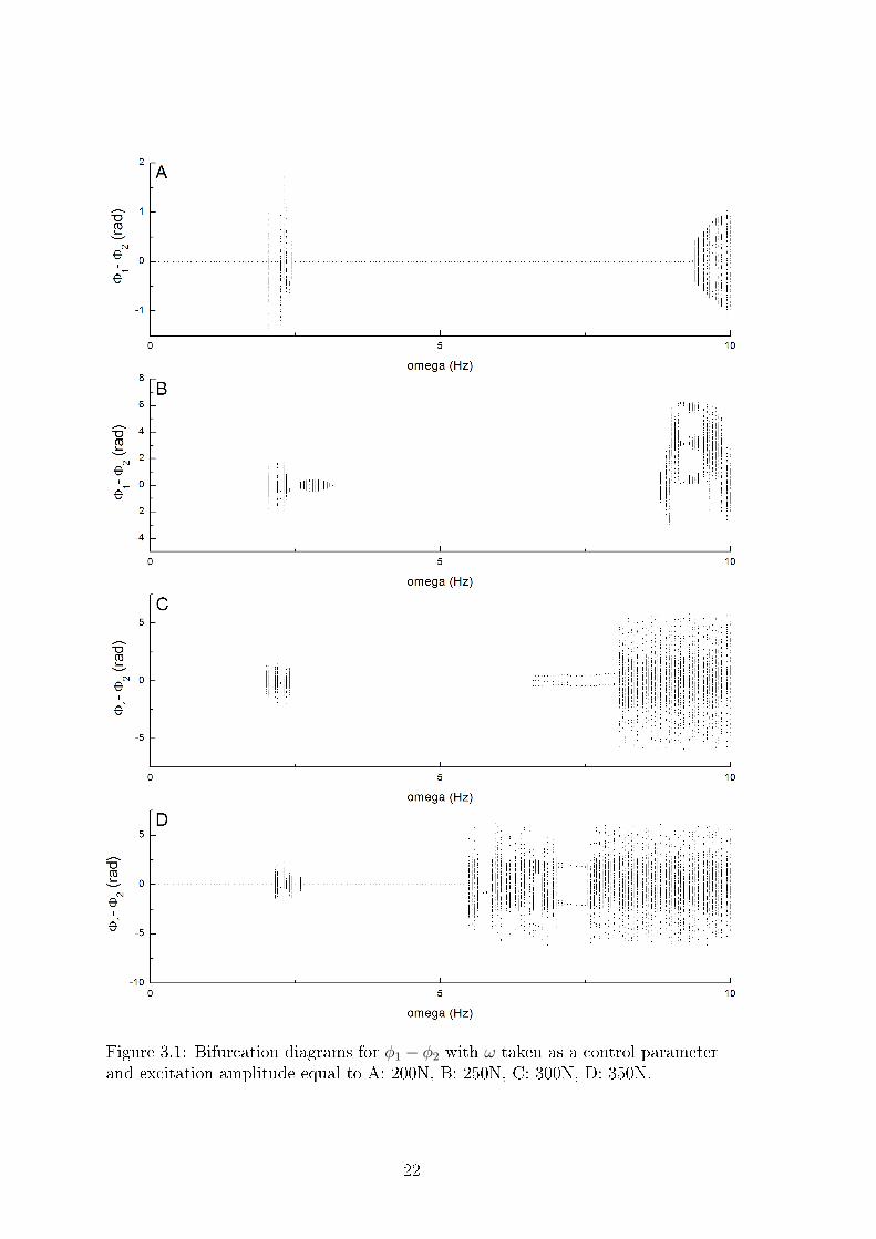
Figure 3.1: Bifurcation diagrams for φ1 − φ2 with ω taken as a control parameterand excitation amplitude equal to A: 200N, B: 250N, C: 300N, D: 350N.
22

Figure 3.2: Bifurcation diagrams for φ3 − φ4 with ω taken as a control parameterand excitation amplitude equal to A: 200N, B: 250N, C: 300N, D: 350N.
23

Figure 3.3: Bifurcation diagrams for φ1 to φ4 and x with ω taken as a controlparameter and amplitude of excitation F = 200 [N]
24
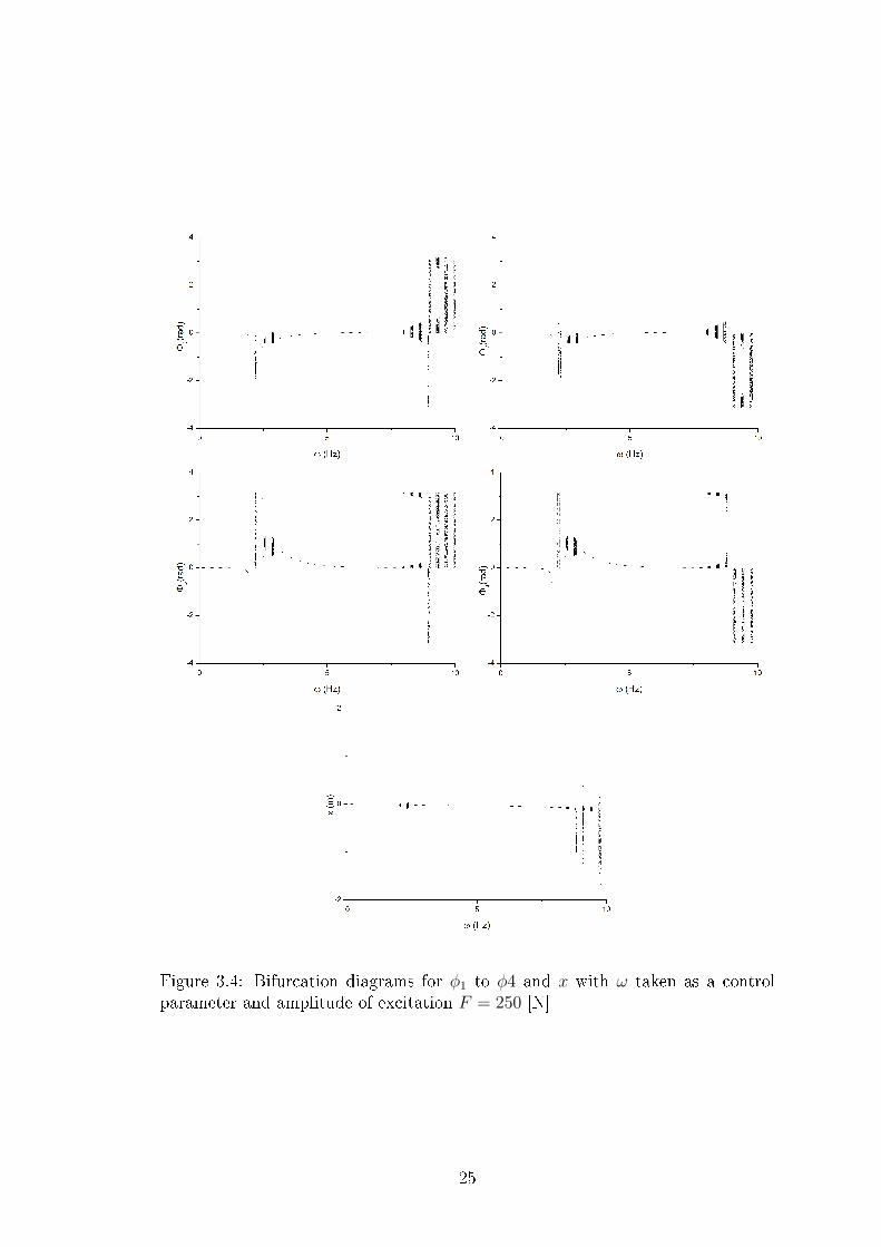
Figure 3.4: Bifurcation diagrams for φ1 to φ4 and x with ω taken as a controlparameter and amplitude of excitation F = 250 [N]
25

Figure 3.5: Bifurcation diagrams for φ1 to φ4 and x with ω taken as a controlparameter and amplitude of excitation F = 300 [N]
26

Figure 3.6: Bifurcation diagrams for φ1 to φ4 and x with ω taken as a controlparameter and amplitude of excitation F = 350 [N]
27
Comparing the bifurcation diagrams for φ1 and φ2 for ω control parameter aswell as the ones for φ3 and φ4 (Figures 3.3, 3.4, 3.5, 3.6) with Figures 3.1 and 3.2respectively, it is noticeable that the range for which the synchronization occurs is therange where the system's behaviour is periodic. The periodic behaviour of the systemis observed when for the given control parameter there is only one point visible onthe bifurcation diagram. This results in a single line if the periodic behaviour occursfor a subsequent control parameter values. When the system behaviour changes intowhat is represented by a regular shape on the bifurcation diagram the pendulums fallout of a complete synchronization. The nature of system's behaviour in those regionswere examined throughly by a set of phase diagrams and Poincaré maps which willbe presented for excitation amplitude F = 250 [N]. The presented phase diagramsand maps were prepared for the regions corresponding to ω = 2.85 [Hz], 8.4 [Hz] and9.5 [Hz]. This will allow to determine wether in for those values of ω the system'sbehaviour is quasiperiodic or chaotic.
The shape of the bifurcation diagram for F = 250 [N] (Figure 3.4) for ω = 2.5[Hz] to ω = 3.1 [Hz] implies the existence of Neimark-Sacker bifurcation, thereforethe phase diagrams and Poincaré maps for ω = 2.85 [Hz]. Subsequently, for the ωvalue over 3.1 [Hz], until 8 [Hz] system seems to be returning to periodic behaviour bymeans of inverse Neimarck-Sacker bifurcation and afterwards once again probably theNeimark-Sacker bifurcation occurs and following the bifurcation the system presumablyfalls into chaotic behaviour by destruction of 3-D Torus, hence the diagrams and mapsfor control parameter equal to 8.4 [Hz] and 9.5 [Hz].
Point ω = 2.85 [Hz] lays in the region of suspected Neiman-Sacker bifurcation.Phase portraits show thick toruses (Figure 3.7). The Poincaré maps in turn showclosed loops (Figure 3.8). This is su�cient to state that at this point the systembehaves in a quasiperiodic way. Quasiperiodic motion at this point con�rms that thechange of system's behaviour visible on the bifurcation diagram for ω in range from2.5 to 3.1 [Hz] is in fact a Neiman-Sacker or as it is also referred to a secondary Hopfbifurcation. This kind of bifurcation can be seen on bifurcation diagrams concerningboth upper (displacements φ1, φ2), and lower (displacements φ3, φ4) pendulums, butnot for the beam.
28

Figure 3.7: Phase portraits for ω=2.85 [Hz] with excitation amplitude F=250 [N]
29

Figure 3.8: Poincaré maps for ω=2.85 Hz with excitation amplitude F=250 N
30

Figure 3.9: Phase portraits for ω=8.4 Hz with excitation amplitude F=250 N
31
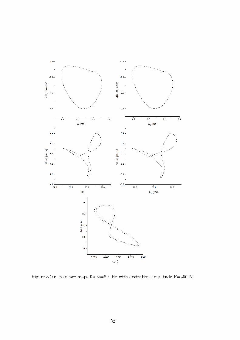
Figure 3.10: Poincaré maps for ω=8.4 Hz with excitation amplitude F=250 N
32

Figure 3.11: Phase portraits for ω=9.5 Hz with excitation amplitude F=250 N
33

Figure 3.12: Poincaré maps for ω=9.5 Hz with excitation amplitude F=250 N
34

Next point, which corresponds to ω = 8.4 [Hz] also lies in the area of suspectedNeiman-Sacker bifurcation and once again, the quasiperiodic motion at this pointwould con�rm this kind of bifurcations. The Poincaré maps for this excitation fre-quency (Figure 3.10) show closed loops for upper and lower pendulum's displacementswhile phase portraits show quite complicated loops. In this case it is also a su�cientproof that there is a quasiperiodic motion at this point, which in turn proves the as-sumption that the change of system's behaviour, visible on bifurcation diagrams forthe displacements of pendulums (Figure 3.4), for a control parameter in range from 8[Hz] to around 8.65 [Hz] is the Neiman-Sacker bifurcation.
The next point was taken for the value ω = 9.5 [Hz] which corresponds to thearea on bifurcation diagrams which can suggest the chaotic behaviour of the system.Phase portrait for this point shows very complicated shape and Poincaré map presentscollection of irregularly distributed points. This can mean that for values of ω higherthan 8.65 system starts to behave hyperchaotically because there is no fractal structurein the plot.
This also con�rms that system stops being in complete synchronization for anypair of the pendulums when it is behaving chaotically for F = 250 [N].
Next step in the analysis of this system was to perform bifurcation diagrams withmass of the upper pendulums (m1) as a control parameter, for chosen values of exci-tation frequency ω. For all excitation amplitude values it was 4 [Hz], additionally 9.8[Hz] for F = 200 [N], 9.4 [Hz] for F = 250 [N], 9 [Hz] for F = 300 [N], 6.3 and 7.3for F = 350 [N].
It can be noticed that for ω = 4HZ, the bifurcation diagrams sets for all of theexcitation amplitudes given (Figures 3.13, 3.15, 3.17 and 3.19) look similar. For thisexcitation frequency doesn't in�uence the system's behaviour for any of the analysedexcitation amplitude, as it is clearly visible that for any angular displacement there isnot more than one point for any chosen value of control parameter. Therefore systemis behaving periodically for excitation frequency ω = 4 [Hz] regardless of mass andexcitation frequency within analysed range.
On the bifurcation diagrams set for ω = 9.8 Hz and F = 200 [N] (Figure 3.14)it can be seen that system behaves periodically only for a small range of controlparameter. Around m1 = 0.7 kg system's behaviour changes and then changes againafter m1 equal to around 1.5 kg into presumably a quasiperiodic behaviour. Also,for lower pendulums, for m1 after around 4.3 kg it falls into what could be a chaoticbehaviour. The further study of this and all of the further cases could fully determinethe behaviour of the system after the changes in the bifurcation diagrams.
For ω = 9.4 and F = 250 [N] (Figure 3.16) the bifurcation diagrams show thatfor those conditions the system can behave periodically but only for a short rangeof upper pendulums mass. System also can behave in a quasiperiodic way for upperpendulums which can be visible for example for m1 > 1.2 kg up until around 5 kg. Forthe lower pendulums system almost instantly falls into presumably chaotic behaviourand remains in this state for the whole range of analysed control parameter.
Analysing the bifurcation diagram for ω = 9 [Hz] and F = 300 [N] (Figure 3.18)it can be noticed that after short region of periodic behaviour for a very light upperpendulums the system falls into supposed chaotic behaviour and remains chaotic forthe whole rest of the control parameter range.
35
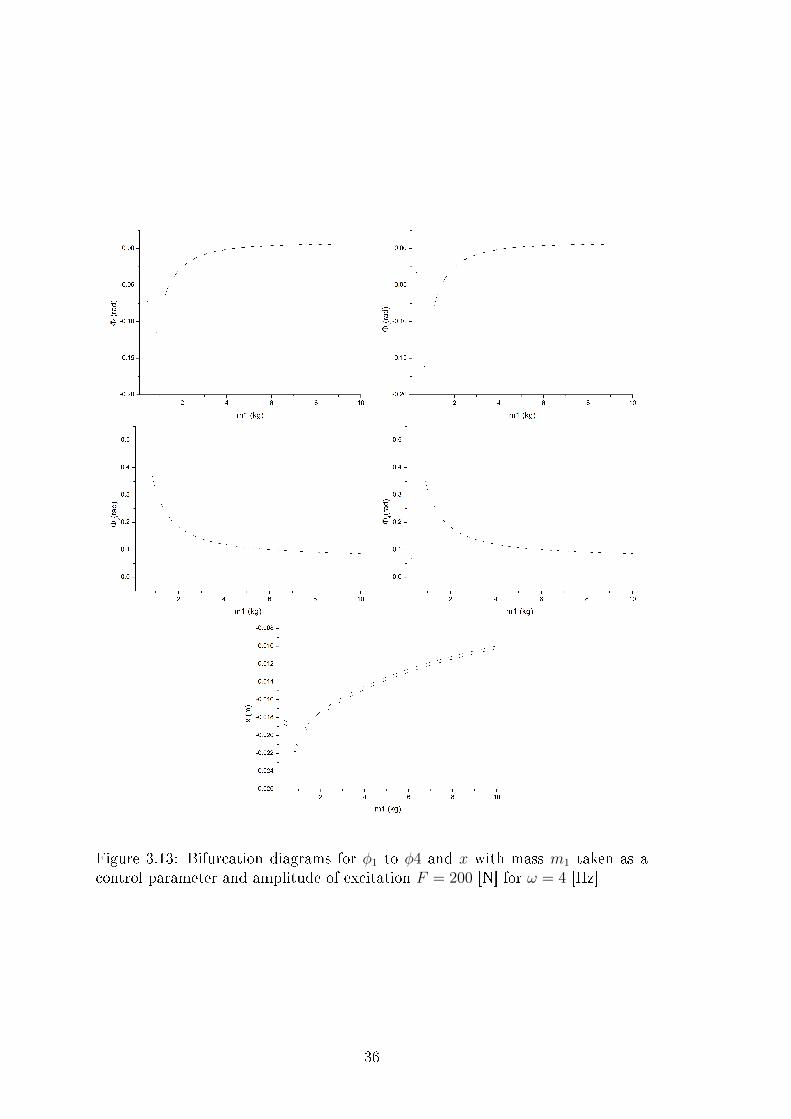
Figure 3.13: Bifurcation diagrams for φ1 to φ4 and x with mass m1 taken as acontrol parameter and amplitude of excitation F = 200 [N] for ω = 4 [Hz]
36

Figure 3.14: Bifurcation diagrams for φ1 to φ4 and x with mass m1 taken as acontrol parameter and amplitude of excitation F = 200 [N] for ω = 9.8 [Hz]
37

Figure 3.15: Bifurcation diagrams for φ1 to φ4 and x with mass m1 taken as acontrol parameter and amplitude of excitation F = 250 [N] for ω = 4 [Hz]
38

Figure 3.16: Bifurcation diagrams for φ1 to φ4 and x with mass m1 taken as acontrol parameter and amplitude of excitation F = 250 [N] for ω = 9.4 [Hz]
39

Figure 3.17: Bifurcation diagrams for φ1 to φ4 and x with mass m1 taken as acontrol parameter and amplitude of excitation F = 300 [N] for ω = 4 [Hz]
40

Figure 3.18: Bifurcation diagrams for φ1 to φ4 and x with mass m1 taken as acontrol parameter and amplitude of excitation F = 300 [N] for ω = 9 [Hz]
41

Figure 3.19: Bifurcation diagrams for φ1 to φ4 and x with mass m1 taken as acontrol parameter and amplitude of excitation F = 350 [N] for ω = 4 [Hz]b
42

Figure 3.20: Bifurcation diagrams for φ1 to φ4 and x with mass m1 taken as acontrol parameter and amplitude of excitation F = 350 [N] for ω = 6.3 [Hz]
43
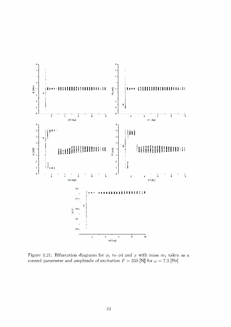
Figure 3.21: Bifurcation diagrams for φ1 to φ4 and x with mass m1 taken as acontrol parameter and amplitude of excitation F = 350 [N] for ω = 7.3 [Hz]
44
As for the analysis of the diagrams concerning the highest analysed excitationamplitude, F = 350 [N], the bifurcation diagrams for ω = 6.3 (Figure 3.20), whichcorresponds to the chaotic behaviour on the bifurcation diagrams with ω taken asa control parameter (Figure 3.6, show that system also presents periodic behaviourfor very light pendulums and subsequently, after what probably is a Neimark-Sackerbifurcation it exhibits a chaotic behaviour for all the angular displacements.
Lastly, the bifurcation diagrams for ω = 7.3 [Hz] and F = 350 [N], which corre-sponds to the window with period two on the Figure 3.6, shows that system behavesin a quasiperiodic way most of the time, whereas at the beginning of the tested range,after brief period of periodic motion and supposed Neimark-Sacker bifurcation fallsinto chaotic behaviour for a short range of m1.
45

Chapter 4
Conclusions
The system under consideration was a set of two double pendulums connected by singledegree of freedom beam excited horizontally. The system has �ve degrees of freedom -horizontal displacement of the beam x and four angular displacements corresponding tofour pendulums (φ1 to φ4). The system analysis was performed using phase portraits,Poincaré maps and bifurcation diagrams, based on the results of numerical calculationsby a program written in C++.
The aim of those analysis was to check the system's behaviour undergoes alongwith the change of the excitation frequency and pendulums mass. The analysis ofsystem's synchronization dependency on excitation was also performed. Both analysiswere performed for four di�erent excitation amplitudes.
For the tested range of control parameter (ω from 0.1 to 10 [Hz]) the synchroniza-tion of the system was changing in a signi�cant way. Although for lower excitationamplitudes both pendulum pairs stayed completely synchronised for most part of theconsidered range, it started to fall out of synchronization for higher ω values. For thehighest excitation amplitude (F = 350 [N]) the system desynchronized slightly afterthe middle of the tested range of control parameter.
The examined system presented di�erent types of behaviour - periodic, quasiperi-odic and chaotic. The type of system's behaviour was checked using bifurcationdiagrams and, additionally, phase portraits and Poincaré maps in order to con�rm thenature of systems behaviour where bifurcation diagrams were not enough. The systemwas throughly analysed for excitation amplitude F = 250 [N] and ω taken as a controlparameter, where all three types of behaviour could be observed. The quasiperiodicbehaviour of the system for this excitation amplitude and control parameter indicatesthe Neimark-Sacker bifurcation. After analysis and comparison of bifurcation dia-grams for angular displacements and phase di�erences it is possible to state that forthis conditions the system is in complete synchronization when it is behaving in aperiodic way and loses synchronization when the system starts to behave chaoticallyor hyperchaotically.
Apart from bifurcation diagrams with excitation frequency the ones with mass ofthe upper pendulums taken as a control parameter were performed. The analysis ofthose digrams shows that although the system's behaviour for ω = 4 [Hz] stays periodicfor the whole analysed range of pendulums mass (0.1 to 10 [kg]). For higher values ofexcitation frequency the system can exhibit periodic, quasiperiodic and (hyper)chaoticbehaviour.
46
Bibliography
[1] Kuznetsov Yuri A. and Sacker Robert J. Neimark sacker bifurcation. Website, 2008.http://www.scholarpedia.org/article/Neimark-Sacker_bifurcation.
[2] Baker L. G. and Blackburn A. J. The pendulum: a case study in physics. Oxford UniversityPress, 2005.
[3] Czolczynski K., Perlikowski P., Stefanski A., and Kapitaniak T. Huygens' odd sympathy
experiment revisited. World Scienti�c Publishing Company, 2010.
[4] Boccaletti S., Kurths J., Osiponov G., Valladeres D. L., and Zhou C. S. The synchro-
nization of chaotic systems. Elsevier, 2000.
[5] Kapitaniak T. and Wojewoda J. Bifurkacje i chaos. Politechnika �ódzka, Wydawnictwonaukowe PWN, 2000.
47

48

List of Figures
1.1 Attractor A and its basin of attraction b(A) . . . . . . . . . . . . . . . 31.2 Attractors: a) stable; b) asymptotically stable . . . . . . . . . . . . . . 41.3 Poincaré map construction . . . . . . . . . . . . . . . . . . . . . . . . 41.4 Saddle-node bifurcation . . . . . . . . . . . . . . . . . . . . . . . . . 61.5 The behaviour of the phase trajectories before Hopf bifurcation . . . . 81.6 The behaviour of the phase trajectories after Hopf bifurcation . . . . . 91.7 Limit cycle created as a result of Hopf bifurcation . . . . . . . . . . . 9
2.1 Two double pendulums coupled by a beam . . . . . . . . . . . . . . . 122.2 System composed of a double pendulum . . . . . . . . . . . . . . . . 132.3 System composed of two pendulums - potential energy . . . . . . . . . 15
3.1 Bifurcation diagrams for φ1 − φ2 with ω taken as a control parameterand excitation amplitude equal to A: 200N, B: 250N, C: 300N, D: 350N. 22
3.2 Bifurcation diagrams for φ3 − φ4 with ω taken as a control parameterand excitation amplitude equal to A: 200N, B: 250N, C: 300N, D: 350N. 23
3.3 Bifurcation diagrams for φ1 to φ4 and x with ω taken as a controlparameter and amplitude of excitation F = 200 [N] . . . . . . . . . . 24
3.4 Bifurcation diagrams for φ1 to φ4 and x with ω taken as a controlparameter and amplitude of excitation F = 250 [N] . . . . . . . . . . 25
3.5 Bifurcation diagrams for φ1 to φ4 and x with ω taken as a controlparameter and amplitude of excitation F = 300 [N] . . . . . . . . . . 26
3.6 Bifurcation diagrams for φ1 to φ4 and x with ω taken as a controlparameter and amplitude of excitation F = 350 [N] . . . . . . . . . . 27
3.7 Phase portraits for ω=2.85 [Hz] with excitation amplitude F=250 [N] . 293.8 Poincaré maps for ω=2.85 Hz with excitation amplitude F=250 N . . 303.9 Phase portraits for ω=8.4 Hz with excitation amplitude F=250 N . . . 313.10 Poincaré maps for ω=8.4 Hz with excitation amplitude F=250 N . . . 323.11 Phase portraits for ω=9.5 Hz with excitation amplitude F=250 N . . . 333.12 Poincaré maps for ω=9.5 Hz with excitation amplitude F=250 N . . . 343.13 Bifurcation diagrams for φ1 to φ4 and x with mass m1 taken as a
control parameter and amplitude of excitation F = 200 [N] for ω = 4[Hz] . . . . . . . . . . . . . . . . . . . . . . . . . . . . . . . . . . . . 36
3.14 Bifurcation diagrams for φ1 to φ4 and x with mass m1 taken as acontrol parameter and amplitude of excitation F = 200 [N] for ω = 9.8[Hz] . . . . . . . . . . . . . . . . . . . . . . . . . . . . . . . . . . . . 37
3.15 Bifurcation diagrams for φ1 to φ4 and x with mass m1 taken as acontrol parameter and amplitude of excitation F = 250 [N] for ω = 4[Hz] . . . . . . . . . . . . . . . . . . . . . . . . . . . . . . . . . . . . 38
49

3.16 Bifurcation diagrams for φ1 to φ4 and x with mass m1 taken as acontrol parameter and amplitude of excitation F = 250 [N] for ω = 9.4[Hz] . . . . . . . . . . . . . . . . . . . . . . . . . . . . . . . . . . . . 39
3.17 Bifurcation diagrams for φ1 to φ4 and x with mass m1 taken as acontrol parameter and amplitude of excitation F = 300 [N] for ω = 4[Hz] . . . . . . . . . . . . . . . . . . . . . . . . . . . . . . . . . . . . 40
3.18 Bifurcation diagrams for φ1 to φ4 and x with mass m1 taken as acontrol parameter and amplitude of excitation F = 300 [N] for ω = 9[Hz] . . . . . . . . . . . . . . . . . . . . . . . . . . . . . . . . . . . . 41
3.19 Bifurcation diagrams for φ1 to φ4 and x with mass m1 taken as acontrol parameter and amplitude of excitation F = 350 [N] for ω = 4[Hz] . . . . . . . . . . . . . . . . . . . . . . . . . . . . . . . . . . . . 42
3.20 Bifurcation diagrams for φ1 to φ4 and x with mass m1 taken as acontrol parameter and amplitude of excitation F = 350 [N] for ω = 6.3[Hz] . . . . . . . . . . . . . . . . . . . . . . . . . . . . . . . . . . . . 43
3.21 Bifurcation diagrams for φ1 to φ4 and x with mass m1 taken as acontrol parameter and amplitude of excitation F = 350 [N] for ω = 7.3[Hz] . . . . . . . . . . . . . . . . . . . . . . . . . . . . . . . . . . . . 44
50