Quantum Motion on Shape Space and the Gauge Dependent Emergence ofDynamics and Probability in Absolute Space and Time

Detlef Durr,1 Sheldon Goldstein,2 and Nino Zanghı3

1Mathematisches Institut der Universitat Munchen, Theresienstraße 39, 80333 Munchen, Germany2Departments of Mathematics and Physics, Hill Center, Rutgers University,

110 Frelinghuysen Road, Piscataway, NJ 08854-8019, USA3Dipartimento di Fisica, Universita di Genova,

Via Dodecaneso 33, 16146 Genova, Italy& Istituto Nazionale di Fisica Nucleare (Sezione di Genova)

(Dated: August 30, 2019)

Relational formulations of classical mechanics and gravity have been developed by Julian Barbourand collaborators. Crucial to these formulations is the notion of shape space. We indicate here thatthe metric structure of shape space allows one to straightforwardly define a quantum motion, aBohmian mechanics, on shape space. We show how this motion gives rise to the more or lessfamiliar theory in absolute space and time. We find that free motion on shape space, when lifted toconfiguration space, becomes an interacting theory. Many different lifts are possible correspondingin fact to different choices of gauges. Taking the laws of Bohmian mechanics on shape space asphysically fundamental, we show how the theory can be statistically analyzed by using conditionalwave functions, for subsystems of the universe, represented in terms of absolute space and time.

Dedicated to Joel Lebowitz, an invaluable friend and colleague

CONTENTS

I. Introduction 2

II. Shape Space 4A. Shapes 4B. Metrics on Shape Space 4C. Best-Matching 5D. Conformal Factors 5

III. Classical Motion on Shape Space 6A. Geodesic Motion 6B. Motion in a Potential 6

IV. Quantum Motion on Shape Space 6A. Bohmian Mechanics 6B. Bohmian Motion on a Riemannian

Manifold 7C. Bohmian Motion on Shape Space 7

V. The Emergence of Absolute Space and Time inthe Classical Case 8A. Gauge Freedom in the Classical Case 8B. Classical Motion in the Newton Gauge 8C. Some Remarks on Relational Space and

Relational Time 9D. Newtonian Gravitation 10E. Gauge Freedom, Symmetry Breaking, and

Newton’s Bucket 10

VI. The Emergence of Absolute Space and Time inthe Quantum Case 10A. Gauge Freedom in the Quantum Case 10B. The Schrodinger Gauge 10

C. Proofs of the Transitions to the DifferentHamiltonians 12

D. Remarks on the Bohmian Motion in theVarious Gauges 14

E. Derivation of the Shape Jacobian 14F. Computation of the Shape Jacobian 16G. More Gauge Freedom 17H. The Canonical Conformal Factor 17

VII. Subsystems 18A. Conditional Wave Functions 18B. Subsystems and the Role of Projectivity 18C. The Emergence of Metrical Time 19

VIII. Probability 19A. Bohmian Mechanics and Probability 19B. The Problem of Non-Normalizable

Measures 19C. The Fundamental Conditional Probability

Formula for Evolving Wave Functions 20D. The Physical Significance of the Conditional

Distribution for Stationary WaveFunctions 22

E. The Association Between Measures on PathSpace and on Configuration Space 23

F. A Conditional Probability Formula for PathSpace Measures 24

G. The Fundamental Conditional ProbabilityFormula for Stationary Wave Functions 24

H. Typicality 24

IX. Outlook 25

Acknowledgments 26

arX

iv:1

808.

0684

4v2

[qu

ant-

ph]

29

Aug

201

9

2

Appendix: Some facts about second-orderpartial differential operators 26

References 26

I. INTRODUCTION

Julian Barbour and Bruno Bertotti, in a very inspiringand influential paper published at the beginning of theeighties [3] (for a recent overview, see [5], [20] and refer-ences therein, see also [1]), transformed a long standingphilosophical controversy about the nature of space andtime into a well-defined physical problem. The philo-sophical issue dates back to the dispute between IsaacNewton, who favored and argued for the need of an ab-solute theory of space and time, and Gottfried WilhelmLeibniz, who insisted upon a relational approach, alsodefended by Ernst Mach in the 19th century. The physi-cal problem put forward by Barbour and Bertotti can beexplained by means of a very elementary and simplifiedmodel of the universe.

Suppose we are given the configuration of a universeof N particles. And suppose we translate every particleof the configuration in the same direction by the sameamount. From a physical point of view it seems rathernatural to take the relational point of view that the twoconfigurations of the universe so obtained are physicallyequivalent or identical. Similarly for any rotation. Go-ing one step further, one regards two configurations ofthe universe differing only by a dilation, i.e. by a uni-form expansion or contraction, as representing in factthe same physical state of the universe. The space ofall genuinely physically different possible configurationsso obtained—taking into account translations, rotations,and dilations—is usually called shape-space. The nameshape-space is indeed natural: only the shape of a con-figuration of particles is relevant, not its position or ori-entation or overall size.

Given a kinematics based on shapes, the next questionto be addressed is that of their dynamics. In their sem-inal paper, Barbour and Bertotti proposed a dynamicalprinciple based on what they called the intrinsic deriva-tive and Barbour now calls best matching, which allowsone to compare two shapes intrinsically, without any ref-erence to the external space in which the particles areembedded. While the intrinsic comparison of shapes iscompatible with positing an absolute Newtonian time asin classical mechanics, it naturally leads to a relationalnotion of time in which global changes of speed of thehistory of the universe give physically equivalent repre-sentations. Then the dynamics can be reduced to ge-ometry in the following sense: a history of the universeis just a curve in shape space without any reference toa special parametrization of the curve given by absoluteNewtonian time.

The goal of the present paper is to extend the forego-ing to the quantum case. We shall do this by considering

the toy model mentioned above in which the universeis modelled as an N -particle system. This will sufficeto highlight the general feature of a relational quantumtheory of the universe. However, we shall do so not byappealing to standard quantization schemes (see e.g., [2],[14]), but by relying on the precise formulation of quan-tum theory provided by Bohmian mechanics [7–9, 11, 12].Steps in this direction have been taken by Vassallo andIp [22] and by Koslowski [17].

Bohmian mechanics is a theory providing a descrip-tion of reality, compatible with all of the quantum for-malism, but free of any reference to observables or ob-servers. In Bohmian mechanics a system of particles isdescribed in part by its wave function, evolving accordingto Schrodinger’s equation, the central equation of quan-tum theory. However, the wave function provides onlya partial description of the system. This description iscompleted by the specification of the actual positions ofthe particles. The latter evolve according to the “guidingequation,” which expresses the velocities of the particlesin terms of the wave function. Thus in Bohmian me-chanics the configuration of a system of particles evolvesvia a deterministic motion choreographed by the wavefunction.

Given the primary role of configurations, as opposed tooperators and canonical quantization relations, it shouldnot come as a surprise that Bohmian mechanics can bevery easily formulated on shape space: a wave functionon shape space will govern the motion of a shape accord-ing to a guiding law analogous to the one of standardBohmian mechanics. And to express the guiding law, aswell as to write down Schrodinger’s equation on shapespace, all one needs is a metric on shape space.

Surprisingly (or maybe not), the properties of metricson shape space have been investigated by applied mathe-maticians before the paper of Barbour and Bertotti, andfor completly different reasons. What in physics is a con-figuration of N particles, in statistics is a set of data,and data analysis often requires that all information in adata set about its location, scale, and orientation be re-moved, so that the information that remains provides anintrinsic description of the shape of the data. Indeed, thename “shape space” is due to the mathematicians thathave been working on these problems of data analysis. Inparticular David G. Kendall, whose early work on shapespace dates back to the 1970s, was concerned with shapein archaeology and astronomy and also considered themotion of shapes formed by independent Brownian par-ticles [15], while Fred Bookstein at about the same timebegan to study shape-theoretic problems in the particu-lar context of zoology. Both recognized that the space ofshapes can be represented by Riemannian manifolds (see[16, 21] for more background). We shall briefly reviewhow to construct a metric on shape space in Sect. II.

Not only in Bohmian mechanics, but also in the clas-sical theory of Barbour and Bertotti, a metric on shapespace plays a pivotal role in the formulation of the the-ory. Indeed, it turns out that Barbour’s best-matching

3

principle is equivalent to a characterization of the dynam-ics as geodesic motion in shape space. Though this factwas acknowledged by the authors in their original paper(and also in more recent publications by Barbour andcollaborators), we think that sufficient emphasis has notbeen given to it. Usually, classical motion on shape spaceis characterized by means of Lagrangian or Hamiltonianformulations with constraints (see, e.g., [4]). While weagree that such methods of analytical mechanics couldbe useful in the analysis of the theory, we think thatthey obscure the geometrical structure of the theory. Soin Sect. III we shall provide a self-contained presenta-tion of the classical theory by emphasizing its geometricalcontent, in particular that the dynamics of shapes (evenin presence of interactions) is geodesic motion on shapespace. In Sect. IV we shall develop the Bohmian theoryof motion and highlight the similarities and differencesbetween the classical case and the quantum case.

An important point that we think has not been givensufficient emphasis is that the fundamental formulationsof the theories—classical or quantum —are in shapespace. And when the theories are formulated in shapespace, one should consider first the simplest ones, namelythe “free” theories based only on the geometrical struc-tures provided by the metric, without invoking any po-tential. This is in contrast with theories formulated inabsolute space, for which free theories can’t begin to ac-count for the experimental data. It is then natural to ask:when we represent the theories in absolute space, whatform do the laws of motion take? Is the representationunique or are there various representations yielding dif-ferent looking laws of motion, some unfamiliar and somemore or less familiar? Moreover do interacting theoriesemerge with nontrivial interactions, although in shapespace the motion is free?

To answer these questions it is helpful to represent ab-solute configuration space in geometrical terms as a fiberbundle, with shape space as base manifold and the fibersgenerated by the similarity group, i.e, by translations,rotations and dilations, which acting on configurationsyields, from a relational point of view, physically equiv-alent states. A representation in absolute configurationspace of the motion in shape space is then given by a“lift” of the motion from the base into the fibers.

Such lifts can rightly be called gauges. In the classicalcase it turns out that in some gauges the law looks un-familiar but there is (at least) one gauge in which, afterperforming a time change (representing indeed anothergauge freedom when also time is seen as relational), thelaw of motion is Newtonian with a potential appearing.The potential depends on the choice of the invariant met-ric (invariant under the action of the similarity group)in absolute configuration space, which we introduce inSect. II, where various possibilities for invariant metricsare given. The classical case is dealt with in Sect. V.

More or less the same is true for the quantum case,where however the gauge yielding ordinary Bohmian me-chanics in absolute configuration space—which we call

the Schrodinger gauge—emerges only for a stationary,i.e. time-independent, wave function (such as with theWheeler-DeWitt equation) on shape space. This again isin line with regarding time as being relational, with anexternal absolute time playing no physical role.

Also here, while the fundamental physics is givenby a free Bohmian dynamics in shape space, in theSchrodinger gauge potential terms appear. One poten-tial term is determined by the scalar curvature inducedby the invariant metric on absolute configuration space.Another potential term arises from the gauge freedomwe have to lift the Laplace-Beltrami operator from shapespace to absolute configuration space, where an extragauge freedom arises from allowing transformations ofthe lifted wave function. To see the Schrodinger gaugearise, we invoke some mathematical facts from differen-tial geometry. The details are in Sect. VI.

Regarding the motion in shape space as physically fun-damental, we may well conclude from Sect.s V and VIthat the gauge freedom forces us to recognize that whatwe have traditionally regarded as fundamental might infact be imposed by us through our choice of gauge. Thisgauge freedom thus imparts a somewhat Kantian aspectto physical theory.

We next turn to the issue of probability, given by thequantum equilibrium measure |Ψ|2 on shape space. Inassessing the relationship between probability on shapespace and the usual Born-rule probabilities on absoluteconfiguration space (associated with the natural lifts ofthe shape space dynamics to absolute space), we en-counter several problems. First of all, since wave func-tions lifted from shape space are translation and scalinginvariant, they fail to be normalizable. Another source ofnon-normalizability is the transition to the Schrodingergauge. For this gauge to be viable, as stated earlier, thewave function must be time-independent, and such wavefunctions typically fail, as with those of the Wheeler-DeWitt equation, to be normalizable.

So what could the associated non-normalizable “prob-abilities” physically mean? Moreover, the physical mean-ing of these measures would be obscure even if they werenormalizable, since the absolute space degrees of freedomthat transcend the relational ones are not observable, andthe configuration Qt of the universe at “time t,” whosedistribution is supposed to be given by the Born rule, is,as we argue, not physically meaningful.

We address these questions in Sect. VIII, in whichwe examine what should be physically and observation-ally meaningful, and find that the relevant probabilitiesfor these are in fact given by a fundamental conditionalprobability formula (see [11] for its meaning in the fa-miliar Bohmian mechanics), as normalized conditionalprobabilities arising from the non-normalizable quantumequilibrium measure on absolute configuration space. Forthis we use the notion of the wave function of a subsys-tem of shape space, a somewhat tricky business that isdealt with in Sect. VII.

We find in fact, somewhat to our surprise, that the

4

−1 1

z

z

x

y

FIG. 1. Representation of the shape space of 3 particles interms of point z in the complex upper half plane. Note thatthe complex conjugate z represents the same triangle since itcan be obtained from that of z by a rotation in 3-dimensionalEuclidean space.

non-normalizability of the wave function of the universeof quantum cosmology is, from a relational Bohmian per-spective, a virtue rather than a vice.

II. SHAPE SPACE

A. Shapes

The totality of configurations q = (~q1, . . . ,~qN ) of Npoints in Euclidean three-dimensional space forms theconfiguration space QQQ = q = R3N of an N -particlesystem. We shall call QQQ the absolute configuration space.On QQQ act naturally the similarity transformations of Eu-clidean space, namely rotations, translations and dila-tions, since each of them acts naturally on each compo-nent of the configuration vector. The totality of suchtransformations form the group G of similarity transfor-mations of Euclidean space. Since the shape of a config-uration is “what is left” when the effects associated withrotations, translations and dilations are filtered away, thetotality of shapes, i.e., the shape space, is the quotientspace Q ≡ QQQ/G, the set of equivalence classes with re-spect to the equivalence relations provided by the simi-larity transformations of Euclidean space.

As such, shape space is not in general a manifold.To transform it into a manifold some massaging isneeded (e.g., by excluding from QQQ coincidence points andcollinear configurations), but we shall not enter into this.1

Here, we shall assume that the appropriate massaging of

1 For more details on this issue, see, e.g., [18] and reference therein.

QQQ has been performed and that Q is a manifold. Sincethe group of similarity transformations has dimension 7(3 for rotations + 3 for translations + 1 for dilations),the dimension of Q ≡ QQQ/G is 3N − 7.

For N = 1 and N = 2 shape space is trivial (it containsjust a single point). N = 3 corresponds to the simplestnot trivial shape space; it has dimension 3×3−7 = 2. Itis worthwhile to give some details about this latter case.Three points in Euclidean space form a triangle, so shapespace is the space of all triangle shapes, with “triangleshape” meaning now what is usually meant in elemen-tary Euclidean geometry. A nice representation of thisspace is in terms of points in the complex plane (calledBookstein-coordinates in [21]). On the real axis, fix twopoints, say −1 and 1, and put them in correspondencewith two vertices of the triangle. Then the third vertex isin one-to-one correspondence with a complex number inthe upper half plane, as shown in Fig. 1. Note that thetriangles in the lower half plane are equivalent to thosein the upper half plane by a suitable rotation in three di-mensions. The real axis is the boundary of the manifoldand its points represent degenerate collinear triangles.The point at infinity represents the degenerate triangu-lar shape with two coinciding vertices. So the space oftriangle shapes (allowing two coincident vertices but notthree) can be put in correspondence with the the ex-tended half upper complex plane, which, by stereographicprojection, is topologically equivalent to a hemisphere.For N > 3 the topological structure is more complicated(see, e.g., [18]).

B. Metrics on Shape Space

Topology, of course, does not fix a metric. A met-ric should provide more, namely a natural notion of dis-tance on Q. And since each point in Q represents a classof configurations of N particles related by a similaritytransformation, the distance between two elements of Qinduced by the metric should not recognize any absoluteconfigurational difference due to an overall translation, orrotation, or dilation. In other words, it should provide ameasure of the intrinsic difference between two absoluteconfigurations (that is, not involving any considerationregarding how such configurations are embedded in Eu-clidean space).

Although the construction of such a metric is wellknown in the mathematical literature on random shapes[18], we prefer to give a self-contained presentation moresuited for the physical applications. The bottom line isthis: a metric on absolute configuration space QQQ that isinvariant under the group G of similarity transformationsof Euclidean space, given by a suitable “conformal factor”(to be explained below), defines canonically a metric onshape space Q.

To understand why this is so, observe first that ab-solute configuration space QQQ can be regarded as a fiberbundle with each fiber being homeomorphic to G and Q

5

dq

dq?

dqk

dq

q

q q + dq

q + dq

q + dq?

Q

Q

1

FIG. 2. Absolute configuration space QQQ and shape space Q

(for a system of three particles). The fiber above shape qconsists of absolute configurations differing by a similaritytransformation of Euclidean space and thus representing thesame shape q. Real change of shape occurs only by a dis-placement to a neighboring fiber q + dq. Only the orthogonalcomponent dq⊥ of dq represents real change, while the ver-tical displacement dq‖ does not contribute; q + dq⊥ is theabsolute configuration in the fiber above q+dq closest to q inthe sense of the gB-distance (best matching).

being its base space (see Fig. 2). So, if g is a metricinvariant under any element of G, the tangent vectorsat each point q ∈ QQQ are naturally split into “vertical”and “horizontal,” where by “naturally” we mean thatthe splitting itself is invariant under the action of G. Thevertical ones correspond to (infinitesimal) displacementsalong the fiber through q and the horizontal ones arethose that are orthogonal to the fiber, i.e., to the verticalones, according to the relation of orthogonality definedby g. More precisely, if dq is an infinitesimal displace-ment at q, we have

dq = dq‖ + dq⊥ with g(dq‖, dq⊥) = 0

(see Fig. 2), with dq‖ vertical and dq⊥ horizontal.The corresponding Riemannian metric on Q is defined

as follows. Let q be a shape, q be any absolute configu-ration in the fiber above q, and dq be any displacementat q. Since g is invariant under the group G, the lengthof dq⊥ has the same value for all absolute configurationsq above q. Then we may set the length of dq equal tothat of dq⊥ and hence obtain the Riemannian metric gBon Q

gB(dq, dq) = g(dq⊥, dq⊥) . (1)

The subscript B stands for Barbour and Bertotti (as wellas base and best matching, see below).

We shall now outline how to construct an invariantmetric on QQQ. Let ge be the mass-weighted Euclideanmetric on QQQ with positive weights mα, α = 1, . . . , N ,(the masses of the particles), in particle coordinates q =(~q1, . . . ,~qα, . . . ,~qN ) given by

ds2 =

N∑α=1

mαd~qα · d~qα , (2)

i.e., with [ge]ij = mαiδij , where the i-th component refersto the αi-th particle. The corresponding line element is

|dq| =

√√√√ N∑α=1

mαd~qα · d~qα . (3)

The metric defined by (2) is invariant under rotations andtranslations, but not under a dilation q → λq, whereλ is a positive constant. Invariance under dilations isachieved by multiplying |dq|2 by a scalar function f(q)that is invariant under rotations and translations andis homogeneous of degree −2. We call f the conformalfactor. So, for any choice of f ,

g = fge , i.e, g(dq, dq) = f(q)|dq|2 , (4)

is an invariant metric on QQQ, yielding the metric on shapespace

gB(dq, dq) = f(q)|dq⊥|2 . (5)

For the associated line element we shall write

ds = |dq| =√gB(dq, dq) =

√f(q) |dq⊥| . (6)

C. Best-Matching

The distance on Q induced by gB is exactly the oneresulting from applying Barbour’s best matching proce-dure. Consider two infinitesimally close shapes, q andq+ dq, and let q be any absolute representative of q, i.e.,any point in the fiber above q. The gB-distance betweenthese shapes is then given by the g-length of the vectordq such that (i) dq is orthogonal to the fiber above qand (ii) q+ dq is an absolute representative of q+ dq. Itfollows that q + dq is the absolute configuration closestto q in the fiber above q + dq. Thus the gB-distance isthe “best matching” distance.

D. Conformal Factors

Many choices of conformal factors are possible. Onethat was originally suggested by Barbour and Bertotti

6

is2

f(q) = fa(q) ≡

∑α<β

mαmβ

|~qα − ~qβ |

2

. (7)

Another example is

f(q) = fb(q) ≡ L−2 , (8)

where

L2 =∑α

mα~qα2 =

1∑αmα

∑α<β

mαmβ |~qα − ~qβ |2 (9)

with ~qα = ~qα−~qcm , the coordinates relative to the centerof mass

~qcm =

∑αmα~qα∑αmα

. (10)

I ≡ L2 is sometimes called (but the terminology is notuniversal) the moment of inertia of the configuration qabout its center of mass. This quantity is half the traceof the moment of inertia tensor M,

L2 =1

2TrM . (11)

We recall that M = M(q), the tensor of inertia of theconfiguration q about any orthogonal cartesian systemx,y,z with origin at the center of mass of the configurationq, has matrix elements given by the standard formula

Mij =

N∑α=1

mα(ρ2αδij − ραiραj) , (12)

where i, j = x, y, z, ραx ≡ xα, ραy ≡ yα, ραz ≡ zα, andρ2α = x2

α + y2α + z2

α.A choice of conformal factor that has not been consid-

ered in the literature is

f(q) = fc(q) ≡ L−87 (detM)−

17 . (13)

Since detM scales as L6, f(q) given by (13) scales asit should, namely, as L−2. Though at first glance thischoice does not seem natural, it is in fact so natural—once the motion of shapes is analyzed from a quantumperspective, see Sect. VI H—that we shall call fc thecanonical conformal factor.

Finally, we give other two examples:

f(q) = fd(q) ≡∑α<β

mαmβ

|~qα − ~qβ |2(14)

f(q) = fg(q) ≡ L−1∑α<β

mαmβ

|~qα − ~qβ |. (15)

The first one corresponds to a natural modification ofthe Newtonian gravitational potential and the second,discussed in [4], corresponds to a dynamics very close tothat of Newtonian gravity (see Sect. V B and Sect. V D).

2 Here and in the following examples the conformal factors aremodulo dimensional factors.

III. CLASSICAL MOTION ON SHAPE SPACE

A. Geodesic Motion

The metric gB on shape space directly yields a law offree motion on shape space, that is, geodesic motion withconstant speed. More explicitly, this is the motion Q =Q(t) at constant speed along the path that minimizes thelength ∫ q2

q1

|dq| =∫ q2

q1

√f(q) |dq⊥| (16)

over all possible paths connecting two shapes q1 and q2

(if they are sufficiently close). Note that the variationalproblem determines only the path of the motion, but notthe motion in time.

Equivalently, a geodesic motion Q = Q(t) is a motionthat parallel-transports its own tangent vector, so

DQ(t)Q(t) = 0 , (17)

where DQ(t) is the covariant derivative with respect to

the metric gB along the curve Q = Q(t). Given the

initial conditions Q(0) and Q(0), the motion will run at

constant speed v = |Q(0)|.

B. Motion in a Potential

Motion under the effect of the potential V = V (q) isgiven by the obvious modification of (17), namely New-ton’s equation

DQ(t)Q(t) = −∇gBV (Q) , (18)

where ∇gB is the gradient with respect to the metric gB .This is equivalent to a characterization of the motion interms of the Lagrangian

L =1

2gB

(dq

dt,dq

dt

)− V (q) =

1

2

∣∣∣∣dqdt∣∣∣∣2 − V (q). (19)

IV. QUANTUM MOTION ON SHAPE SPACE

A. Bohmian Mechanics

Various quantization schemes have been put forwardin order to provide a quantum theory of motion on shapespace; for a thorough overview, see [1]. These schemesare mostly based on Dirac quantization of classical con-strained systems or on Feynman path integration [14].We shall follow here a novel approach based on Bohmianmechanics. Bohmian mechanics is a completely deter-ministic—but distinctly non-Newtonian—theory of par-ticles in motion, with the wave function itself guiding thismotion. We shall explain below how this theory can be

7

naturally formulated on shape space, after a brief reviewof the main features of the theory.

Bohmian mechanics is the minimal completion ofSchrodinger’s equation, for a non-relativistic system ofparticles, to a theory describing a genuine motion ofparticles. For Bohmian mechanics the state of a sys-tem of N particles is described by its wave functionΨ = Ψ(~q1, . . . ,~qN ) = Ψ(q), a complex- (or spinor-) val-ued function on the space of possible configurations q ofthe system, together with its actual configuration Q de-

fined by the actual positions ~Q1, . . . , ~QN of its particles.The theory is then defined by two evolution laws. One isSchrodinger’s equation

i~∂Ψ

∂t= HΨ , (20)

for Ψ = Ψt, the wave function at time t, where H isthe non-relativistic (Schrodinger) Hamiltonian, contain-ing the masses mk, k = 1, . . . , N , of the particles and apotential energy term V . For spinless particles, it is ofthe form

H = −N∑α=1

~2

2mα

~∇2α + V , (21)

where ~∇α = ∂∂~qα

is the gradient with respect to the posi-

tion of the α-th particle. The other law is the the guidinglaw, which, for spinless particles, is given by the equa-tion3

d~Qαdt

=~mα

Im~∇αΨ

Ψ(~Q1, . . . , ~QN ) (22)

for Q = Q(t), the configuration at time t. For an N -particle system these two equations, together with thedetailed specification of the Hamiltonian H, completelydefine the Bohmian motion of the system. For sake ofsimplicity, we shall consider here just Bohmian mechanicsfor spinless particles, with Hamiltonian (21) and guidinglaw (22). For more details on the formulation of Bohmianmechanics for particles with spin or other internal degreesof freedom, see [12].

While the formulation of Bohmian mechanics doesnot involve the notion of quantum observables, as givenby self-adjoint operators—so that its relationship tothe quantum formalism may at first appear somewhatobscure—it can in fact be shown that Bohmian mechan-ics not only accounts for quantum phenomena, but also

3 The general form of the guiding equation is

d~Qα

dt=

~mα

ImΨ∗ ~∇αΨ

Ψ∗Ψ(~Q1, . . . , ~QN ) .

If Ψ is spinor-valued, the products in numerator and denomina-tor should be understood as scalar products. If external mag-netic fields are present, the gradient should be understood as thecovariant derivative, involving the vector potential.

embodies the quantum formalism itself as the very ex-pression of its empirical import [12, Ch.2 and 3].

It is worth noting that the guiding equation (22) is

intimately connected with the de Broglie relation ~p = ~~k,proposed by de Broglie in late 1923, the consideration ofwhich quickly led Schrodinger to the discovery of his waveequation. The de Broglie relation connects a particleproperty, momentum ~p = m~v, to a wave property, the

wave vector ~k of a plane wave Ψ(~q) = ei~k·~q. From this

one can easily guess the guiding equation as the simplestpossibility for an equation of motion for Q for the caseof a general wave function Ψ.

B. Bohmian Motion on a Riemannian Manifold

Note that, given V , the Bohmian mechanics definedby equations (20), (21), and (22) depends only upon theRiemannian structure g = ge given by (2). In terms ofthis Riemannian structure, the evolution equations (21)and (22) become

dQ

dt= ~ Im

∇gΨΨ

(23)

i~∂Ψ

∂t= −~2

2∆gΨ + VΨ , (24)

where ∆g and ∇g are, respectively, the Laplace-Beltramioperator and the gradient on the configuration spaceequipped with this Riemannian structure. But there isnothing special about this particular Riemannian struc-ture. Indeed, equations (23) and (24) as such hold verygenerally on any Riemannian manifold. Thus, the formu-lation of a Bohmian dynamics on a Riemannian manifoldrequires only as basic ingredients the differentiable andmetric structure of the manifold.

C. Bohmian Motion on Shape Space

Equations (23) and (24) define immediately Bohmianmotion on shape space with Riemannian metric g = gBas the motion on shape space given by the evolution equa-tions

dQ

dt= ~ Im

∇BΨ

Ψ(25)

i~∂Ψ

∂t= −~2

2∆BΨ + V Ψ , (26)

where ∆B and ∇B are, respectively, the Laplace-Beltrami operator and the gradient on the configurationspace equipped with the Riemannian metric (5). Thisis all there is to say about the formulation of Bohmianmechanics on shape space. (This should be contrastedwith more involved approaches as in, e.g., [22].)

8

V. THE EMERGENCE OF ABSOLUTE SPACEAND TIME IN THE CLASSICAL CASE

A. Gauge Freedom in the Classical Case

Given classical motion in shape space, there is a hugehost of motions in absolute space that are compatiblewith it, the only constraint being that they should projectdown to free motion, or the motion (18), in shape space.This freedom of choice is analogous to gauge freedom ingauge theories. Some choices are however more naturalthan others, as we shall discuss below.

B. Classical Motion in the Newton Gauge

A very natural choice of a motion in absolute configu-ration space is the horizontal lift of a motion Q = Q(t) inshape space, that is, a motion Q = Q(t) in absolute con-figuration space that starts at some point q1 on the fiberabove q1 and is horizontal, i.e., the infinitesimal displace-ments dQ are all horizontal. (Note that the final point q2

in the fiber above q2 is then uniquely determined.) Wecall this choice the invariant gauge.

We shall assume V = 0.4 Then the motion in theinvariant gauge is geodesic motion with respect to theinvariant metric (which explains the terminology). Tosee this, observe that it follows from (16) that the lengthof a horizontal lift of a path in shape space is given by∫ q2

q1

√f(q) |dq⊥| =

∫ q2

q1

√f(q) |dq| , (27)

where the equality follows from horizontality of the path.So, the path of a horizontal lifted motion Q = Q(t) hasminimal length over all horizontal paths connecting q1

and q2, but since any non horizontal path has a greaterlength, Q(t) also minimizes the right hand side of (27)over all paths connecting q1 and q2.

We shall now show that by a suitable change of speed,we get to another gauge that we shall call the Newtongauge, a gauge in which the motion is Newtonian, i.e., itsatisfies Newton’s equation F = ma for suitable F . Toestablish this, we first observe that the right hand side of(27) is of the form ∫ q2

q1

√E − V |dq| (28)

for E = 0 and V (q) = −f(q). According to the Jacobiprinciple, (28) is minimized by the path of a Newtonianmotion Q′ = Q′(t) in a potential V and total energy

E =1

2

∣∣∣∣dQ′dt∣∣∣∣2 + V = 0 . (29)

4 Our goal is to show that the simplest dynamics on shape spaceleads to a nontrivial dynamics in a suitable gauge. The caseV 6= 0 will be considered in the next subsection.

Thus the path of a lifted motion Q = Q(t) is the same asthat of a Newtonian motion, but its speed along the pathis different: according to (29) the speed of the Newtonianmotion is ∣∣∣∣dQ′dt

∣∣∣∣ =√

2(E − V ) =√

2f , (30)

while according to (6) the speed of the lifted motion is∣∣∣∣dQdt∣∣∣∣ =

1√f

∣∣∣∣dqdt∣∣∣∣ =

v√f, (31)

with v the constant speed of the motion on shape space.So the two motions are different. But suppose we allowfor a change of the flow of time and replace t with a newtime variable t′ in such a way that the speed of the liftedmotion with respect to this new time variable equals theNewtonian speed

√2f ,∣∣∣∣dQdt′∣∣∣∣ =

∣∣∣∣dQdt dt

dt′

∣∣∣∣ =√

2f ,

whence,

v√f

dt

dt′=√

2f , i.e.,dt′

dt=

v√2f

. (32)

Then Q = Q(t′), the lifted motion with respect to thisnew time variable, is indeed a Newtonian motion, that

is, the particles positions ~Qα, α = 1, . . . , N , forming theconfiguration Q satisfy Newton’s equations

mαd2~Qα

dt′2= −~∇αV (~Q1, . . . ~QN ) . (33)

One may wonder about the status of the time change(32). If one considers time to be absolute, Q = Q(t)and Q′ = Q′(t) are two different motions. But if onetakes a relational view about time, analogous to the rela-tional view about space that we started with, Q = Q(t)and Q′ = Q′(t) are the same motion. In other words, iftime is relational, changes of speed, such as that givenby (32), provide equivalent representations of the samemotion. Accordingly, the use of one time variable insteadof another is a matter of convenience, analogous to thechoice of a gauge. The choice of time variable for whichNewton’s equations (33) hold is the gauge fixing condi-tion that leads from the invariant gauge to the Newtongauge; for the sake of simplicity, from now on we shallcall it t instead of t′.

The invariant gauge has been defined by requiring thatthe path be horizontal. It turns out that this is equivalentto the following conditions:

N∑α=1

mαd~Qα = 0 (34)

N∑α=1

mα~Qα × d~Qα = 0 (35)

N∑α=1

mα~Qα · d~Qα = 0 . (36)

9

To see how this comes about, let

δ~Qα = ~ε+~θ × ~Qα + λ~Qα (37)

where ~ε, ~θ, and λ are the infinitesimal parameters of atranslation, a rotation and a dilation respectively, and let

δQ = (δ~Q1 . . . , δ~QN ). Then

Q→ Q+ δQ (38)

is an infinitesimal vertical transformation. Since the in-finitesimal motion displacement dQ is purely horizontal,it must be orthogonal to δQ, i.e., g(dQ, δQ) = 0, whichimplies that

~ε·N∑α=1

mαd~Qα+~θ·N∑α=1

mα~Qα×d~Qα+λ

N∑α=1

mα~Qα·d~Qα = 0 .

This equality is satisfied (for all ε, ~θ, and λ) only if the

terms multiplying ~ε, ~θ, and λ are separately zero, whence(34), (35), and (36).

The constraints (34), (35), and (36) have a naturalmeaning for a theory aimed at describing the universeas a whole. So to speak, they minimize the amount ofmotion when the universe is described in the invariantgauge.

Moreover, the constraints (34) and (36) are equivalent,respectively, to the requirements that the motion Q(t)

is such that the center of mass (∑mα)−1

∑mα

~Qα and

the moment of inertia about the origin∑mα

~Q2α don’t

change. Clearly, these are natural gauge fixing choicescorresponding to translational and dilational (scaling)symmetry. However, there can be no function on ab-solute configuration space which corresponds in a similarway to (35). The constraint (35) does not correspondto the constancy of a function on absolute configurationspace.5

In the Newton gauge, (34), (35), and (36) can be ex-

pressed in terms of the familiar total momentum ~P, total

angular momentum ~J and (maybe less familiar) dilationalmomentum D as

~P =N∑α=1

mαd~Qαdt

= 0 (39)

~J =

N∑α=1

mα~Qα ×

d~Qαdt

= 0 (40)

D =

N∑α=1

mα~Qα ·

d~Qαdt

= 0 . (41)

5 This corresponds to the fact that the subspaces of the tangentspaces (at the points in absolute configuration space) orthogonalto the fibers don’t correspond to a foliation of absolute configu-ration space into submanifolds orthogonal to the fibers. This isrelated to the fact that the curvature of the connection relatingthe tangent spaces sitting at different points is non-vanishing andthis, in its turn, is related to the Berry phase.

C. Some Remarks on Relational Space andRelational Time

The first simple moral to draw form the foregoing isthat free motion on shape space, i.e., for interaction en-ergy V = 0, leads to interaction energy V 6= 0 in theNewton gauge and so to an interacting particle dynamicsin absolute spacetime (governed by Newton’s laws (33)).In other words, the geometry on shape space defined bythe conformal factor f manifests itself as potential energyV among the particles in the Newton gauge.

This remarkable fact is a direct consequence of the twomain features of the theory under consideration. One isour starting point, namely that shape space is fundamen-tal, that is, that space is relational. The other one hasemerged in the analysis of how shape dynamics appearsin the Newton gauge: motions following the same pathwith different speeds are indeed the same motion. Andthis corresponds to time being relational.

This remarkable fact notwithstanding, one may stillwonder what sort of motion in absolute space correspondsto a shape dynamics with potential energy V 6= 0. To an-swer to this question, let us go back to equations (18) or(19) defining interacting motion in shape space. Clearly,these equations are not in harmony with relational time:the acceleration in the LHS of (18) or the Euler-Lagrangeequations arising from (19) rely on absolute time. Onthe other hand, the characterization of motion in termsof the Jacobi principle fits nicely with relational time.Adapted to the present case, this principle says that thepath followed by a motion in shape space is the path thatminimizes ∫ q2

q1

√E − V |dq| , (42)

where E is any given fixed constant. And this is in com-plete harmony with relational time: if time is relationalall that matters is the path and not the speed along thepath. Note, however, that for the relational dynamicsdefined by (42) changing the potential by adding a con-stant changes the dynamics, unlike the dynamics definedby (18) or (19).

Moreover, if interacting motion is defined according to(42), it will still be free motion, although with respectto a different metric: the one defined by the conformalfactor fE ,V = (E − V )f (with V (q) = V (q), for anypoint q on the fiber above q). As for the starting questionconcerning how the motion appears in the Newton gauge,the answer is rather obvious: just as above, but now forthe conformal factor fE ,V = (E − V )f .

The motion on shape space characterized by (42) is de-fined for any potential V on shape space; in particular, itis defined for V + E . So the constant E can be absorbedin the potential; that is, without any loss of generality, wemay set E = 0 and consider only fV = −V f . In this re-gard, it is important to observe that changing the poten-tial by a constant changes the conformal factor and thus

10

changes the dynamics. This is a peculiar aspect of rela-tional mechanics (relational space and relational time),as opposed to the usual Newtonian mechanics (absolutespace and absolute time), where a change of the potentialby a constant does not change Newton’s laws.

D. Newtonian Gravitation

In the previous sections we found that in the Newtongauge, when the physical law on shape space is free mo-tion (or even non-free motion), the potential V = −fappears, where f is the conformal factor. We mentionedsome choices for f in Sect.II D. No such choices, which arenecessarily functions homogenous of degree −2, seem toyield exactly the Newtonian gravitational potential Ug.While we believe the detailed exploration of the impli-cations of the models discussed here is worthwhile, wenonetheless regard the models explored in this paper,both classical and quantum, as toy models, so that suchan analysis of them, with the expectation of recoveringwell established physics, might be somewhat inappropri-ate or premature.

However, it should be observed that some of the con-formal factors given in Sect. II D, e.g., fa and fg, in-deed give rise to a force law in the Newton gauge that isvery close to that of the Newtonian gravitational poten-tial. Note for example that for the conformal factor fgthe corresponding potential is of the form Vg = L−1Ug,where Ug is the Newton gravitational potential and L inthe Newton gauge is a constant of the motion. The forcearising from this potential adds to the Newtonian force avery small centripetal correction that allows I = L2, themoment of inertia about the center of mass, to remainconstant [4].

E. Gauge Freedom, Symmetry Breaking, andNewton’s Bucket

The structures in an absolute space involved in the for-mulation of the geometry of shape space—in particular,the metric g given by the conformal factor—are invariantunder translations, rotations, and scaling. So, of course,is the classical dynamics on shape space, since, by con-struction, translations, rotations, and scaling act triviallyon shape space. The procedure defining the invariantgauge (Sect. V B) respects all of these symmetries. Butscale invariance is broken in the Newton gauge becausethe time change (32) involved in the transition from theinvariant gauge to the Newton gauge depends on the scalevia f . This illustrates the obvious fact that the symme-tries of the law of motion arising from the fundamentaldynamics on shape space by a choice of gauge dependson the particular details defining that gauge.

A much larger class of symmetries for the shape spacedynamics—also acting trivially—involves an independentgroup action g ∈ G at each “time” (but not so indepen-

dent that smoothness is lost). The most important andfamiliar of these symmetries, when applied in a particulargauge, are uniformly growing translations (correspond-ing to Galilean boosts) and uniformly growing rotations(corresponding to the use of a rotating coordinate sys-tem or frame of reference). The former are a symmetryof the law of motion of the Newton gauge (ignoring theconstraints (39)-(41), which are obviously not preservedunder boosts), since a change in position that dependslinearly on time produces no change in the acceleration.The latter, however, is not a symmetry of the Newtonianlaw of motion.

The behavior of Newton’s bucket, which has been usedto argue against a relational understanding of space,is thus seen, in fact, to be a natural consequence ofthe relational view. That behavior is a consequence ofNewtonian-like laws akin to those that emerge as thedescription in the Newton gauge of the fundamental dy-namics on shape space. However, in the Newton gaugethe total angular momentum of the universe must van-ish, and this is incompatible with a (non-negligible) uni-form rotation of the “fixed stars.” In a gauge correspond-ing to applying a uniformly growing rotation to the mo-tion of the Newton gauge, the Newtonian law of motionis not obeyed, though the motion so obtained remainsentirely compatible with the fundamental dynamics onshape space, a dynamics for which the behavior of thebucket depends essentially on its motion relative to thatof the fixed stars.

VI. THE EMERGENCE OF ABSOLUTE SPACEAND TIME IN THE QUANTUM CASE

A. Gauge Freedom in the Quantum Case

As in the classical case, also the quantum theory isabout shapes, if one takes the standpoint of Bohmianmechanics. In this formulation of quantum mechanics,the role of the wave function is that of governing themotion of shapes. Moreover, as in the classical case, thereis gauge freedom: a huge host of motions in absolute spaceQQQ are compatible with Bohmian motion in shape spaceQ. But now the presence of the wave function makes thefreedom larger and subtler at the same time, as we shallexplain in the following.

B. The Schrodinger Gauge

Let Q = Q(t) be a Bohmian motion in shape space,that is, a solution of (25) with the wave function Ψ beinga solution of Schrodinger’s equation (26) on shape space.For simplicity, we shall assume that V = 0 so that (26)becomes

i~∂ψ

∂t= Hψ , H = −~2

2∆B (43)

11

with ∆B the Laplace-Beltrami operator on shape space.As in the classical case, we wish to characterize motions

in absolute space that are compatible with motions inshape space, that is, motions Q = Q(t) in QQQ that projectdown to Q = Q(t) in Q, i.e., such that

π(Q(t)) = Q(t) , (44)

where π is the canonical projection from QQQ space to Q.Clearly, there are a great many possibilities for compat-ible motions in absolute configuration space.

As in the classical case, one may restrict the possibili-ties by considering natural gauges. And as in the classicalcase where one looks for gauges such that the absolutemotions satisfy Newton’s equations, in the quantum casewe now look for gauges such that the compatible motionson QQQ are themselves Bohmian motions, i.e. motions gen-erated by a wave function in the usual sort of way.

For example, suppose that we proceed as in the classi-cal case and take a horizontal lift of a motion Q = Q(t)in shape space, that is, an absolute motion for which theinfinitesimal displacements dQ are all horizontal. Let usnow consider the lift to QQQ of a wave function Ψ on Q,

namely, the wave function Ψ1 on absolute configurationspace such that

Ψ1(q) = Ψ(q) (45)

for any point q on the fiber above q. Let ∇gbe the gradi-ent with respect to the invariant measure (4). Then the

vector ∇gΨ1(q) in QQQ is horizontal and the motions on QQQdefined by

dQ

dt= ~ Im

∇gΨ1

Ψ1

(46)

are horizontal lifts of motions on Q. So, in the quantumcase, horizontality is immediate.

Let us now consider the time evolution of the liftedwave function Ψ1 on QQQ. Let ∆B be a lift to absoluteconfiguration space of the Laplace-Beltrami operator ∆B

on shape space, namely an operator on QQQ such that

∆BΨ1 = ∆BΨ . (47)

Then

i~∂Ψ1

∂t= H1Ψ1 , with H1 = −~2

2∆B . (48)

It might seem natural to guess that ∆B coincides with∆g, the Laplace-Beltrami operator with respect to g, but

this is wrong; nor is H1 a familiar sort of SchrodingerHamiltonian, with or without a potential term.

While Ψ1 need not obey any familiar Schrodinger-type equation, one may ask whether there exists a gaugeequivalent wave function that does. By gauge equivalent

wave function we mean this: If one writes Ψ1 as Re(i/~)S

one sees that the velocity field given by (46) is just ∇gS,so transformations of the wave function

Ψ1 → Ψ′1 = F Ψ1 , (49)

where F is a positive function, do not change its phaseand thus the velocity.

It turns out that there exists a positive function F

such that Ψ3 = F Ψ1 (why we use 3 here instead of 2will be clearer in Sect. VI C) satisfies a Schrodinger typeequation on absolute configuration space for a suitablepotential V , namely,

i~∂Ψ3

∂t= H3Ψ3 (50)

with

H3 = −~2

2

N∑α=1

~∇α ·1

fmα

~∇α + V (51)

= −~2

2∇ · 1

f∇+ V , (52)

where ∇ and ∇· are the gradient and divergence withrespect to the mass-weighted Eucidean metric (2), i.e.,

∇ =

(1

m1

~∇1, . . . ,1

mN

~∇N)

(53)

and

∇· =(~∇1, . . . , ~∇N

)· . (54)

Here f is the conformal factor, and

V = V1 + V2 (55)

V1 = −~2

2

∆BJ1/2

J1/2(56)

V2 = −~2

2fn4 ∆g

(f−

n4

), (57)

with

J = Lf7/2√

detM , (58)

where L = L(q) is given by equation (9) and M = M(q)is the tensor of inertia of the configuration q about anyorthogonal cartesian system x,y,z with origin in its centerof mass and with matrix elements given by (12), and

where ∆B is the canonical lift (65).We shall now describe what we think is appropriate to

be called the Schrodinger gauge, the true quantum ana-logue of the Newton gauge. If we take into account thattime is relational, as we should, the fundamental equa-tion for the wave function on shape space is presumablythe stationary equation

−~2

2∆BΨ = E Ψ , (59)

12

where, for simplicity, we have set V = 0 and E is anygiven fixed constant (for example E = 0).

As before, let Ψ1 be the lift of Ψ to QQQ, so that Ψ1

satisfies the equation

(H1 − E )Ψ1 = 0 , (60)

with H1 a lift of H as in (48), and the evolution on theabsolute configuration QQQ is still given by (46). But now,for relational time, motions following the same path withdifferent speeds are the same motion. So, in the formulafor the gradient on the right hand side of (46), ∇g =f−1∇, we may regard f as a change of speed defining anew time variable that for the sake of simplicity we shallstill call t (“random time change”). Then in absolutespace the guiding equation (46) becomes

d~Qαdt

=~mα

Im~∇αΨ1

Ψ1

. (61)

Again, Ψ1 need not obey any familiar stationarySchrodinger-type equation. However, as before, we mayexploit gauge freedom to transform (60) into a station-ary Schrodinger-type equation. Indeed, we have an evengreater gauge freedom in changing the wave function andthe Hamiltonian, as will be shown below. In particular,there is a gauge, the Schrodinger gauge, in which (59)becomes

HSΦ = 0 (62)

with

HS = −~2

2∇2 + U , (63)

where ∇2 =∇·∇ is the mass-weighed Euclidean Lapla-cian, and

U = f(V1 − E )− ~2

8

n− 2

n− 1fRg , (64)

where Rg is the scalar curvature of the invariant metric g.

C. Proofs of the Transitions to the DifferentHamiltonians

We shall now provide proofs of the transitions from

Hamiltonian H1 in equations (48) and (60) to Hamilto-

nian H3, given by (52), in equation (50), and Hamilto-

nian HS , given by (63), in equation (62). The materialpresented here and in the following subsections is of amore mathematical character and could be skipped infirst reading.

The lift to QQQ of the Laplace-Beltrami operator ∆B onQ is by no means unique. There is however a “canonicallift” given by the formula

∆B = J divg J−1 gradg , (65)

where J = J(q) is a positive function on QQQ (unique upto a constant multiple), gradg is the gradient, given by(using the Einstein summation convention)(

gradg)i

= gij∂j (66)

in a coordinate basis (∂1, . . . , ∂n), and divg is the diver-gence whose action on a vector field Y = (Y 1, . . . , Y n) inthe coordinate basis (∂1, . . . , ∂n) is

divg Y =1√|g|∂i√|g|Y i , (67)

where |g| = |det(gij)| is the absolute value of the de-terminant of the metric tensor gij in the given local co-ordinates. The existence of a positive J such that (65)defines a lift of ∆B will be proven in Sect. VI E and for-mula (58) for J will be derived in Sect.VI F. We call Jthe shape Jacobian.

While ∆B does not coincide with ∆g, the Laplace-Beltrami operator on QQQ, it is a minimal modificationthereof. Just compare (65) with ∆g as “div-grad” op-erator, i.e., in local coordinates,

∆g = divg gradg =1√|g|∂i√|g|gij∂j (68)

=1

fn/2∇ · f (n/2)−1∇ , (69)

where in the second equality we have made explicitthe invariant metric g = fge, with ge given by (2),in Euclidean particle coordinates: gij = fmαiδij , so

that√|g| = (m1 · · ·mN )

3/2fn/2, with n = 3N , and

gij = f−1m−1αi δij . Similarly,

∆B =J√|g|∂i

√|g|J

gij∂j (70)

=J

fn/2∇ · f

(n/2)−1

J∇ . (71)

Note that ∆g is self-adjoint on L2(dµg), the set of func-tions on QQQ square integrable with respect to the volumeelement defined by the metric g,

dµg =√|g|dx1 · · · dxn ∝ fn/2d3~q1 · · · d3~qN (72)

(n = 3N). In contrast, ∆B is self adjoint with respect tothe volume element dµ = J−1dµg.

Let us now consider the effect of the gauge transforma-

tion (49) on H1 = −(~2/2)∆B . Since Ψ1 → Ψ2 = F Ψ1

is a unitary transformation

U : L2(dµ)→ L2(F−2dµ) , (73)

the effect of (49) is to transform H1 into the unitarilyequivalent operator

H2 = U H1U−1 = F H1F

−1 , (74)

13

so that H1, Ψ1 and H2, Ψ2 provide equivalent descrip-tion of the dynamics.

A natural question is whether there is an equivalent

description such that H2 is Schrodinger-like with somepotential. The key to answering this question is the fol-lowing theorem concerning second order partial differen-tial operators (see the Appendix for a proof): SupposeH1 and H2 are second order partial differential opera-tors, both self-adjoint with respect to the same measure.If they have the same pure 2nd derivative parts then

H2 = H1 + V . (75)

Moreover, if H11 = 0 (no constant part) then V = H21.We first apply this theorem to the operators H1 =

−(~2/2)∆g and H2 = H2, unitarily equivalent to H1 ac-

cording to (74). Choosing F = J−1/2 in (74), H2 isself-adjoint with respect to µg. (According to (73), thisoperator is self-adjoint with respect to Jdµ = JJ−1dµg =dµg.) So, H1 and H2 so defined are self-adjoint withrespect to the same measure, have the same pure 2ndderivative parts (namely, −(~2/2)f−1∇ ·∇) and H11 =0. Thus, according to the theorem stated above,

H2 = −~2

2∆g + V1 (76)

with

V1 = −~2

2

∆BJ1/2

J1/2. (77)

Let us now perform a further transformation on H2 to

make it unitarily equivalent to the operator H3 (see (52)),which is self-adjoint with respect to the Lebesgue mea-sure d3~q1 · · · d3~qN . Observing the form (69) of ∆g, thedesired transformation is

H2 → H3 = fn/4H2f−n/4 (78)

= −~2

2fn/4∆gf

−n/4 + V1 (79)

≡ H2 + V1 . (80)

Consider now the operator

H1 = −~2

2∇ · 1

f∇ (81)

and note that H1 and H2 have the same pure 2nd deriva-tive parts, are self-adjoint with respect to the same mea-sure (the Lebesgue measure) and H11 = 0. Thus,

H2 = H1 + V2 (82)

with

V2 = H21 = −~2

2fn4 ∆g

(f−

n4

). (83)

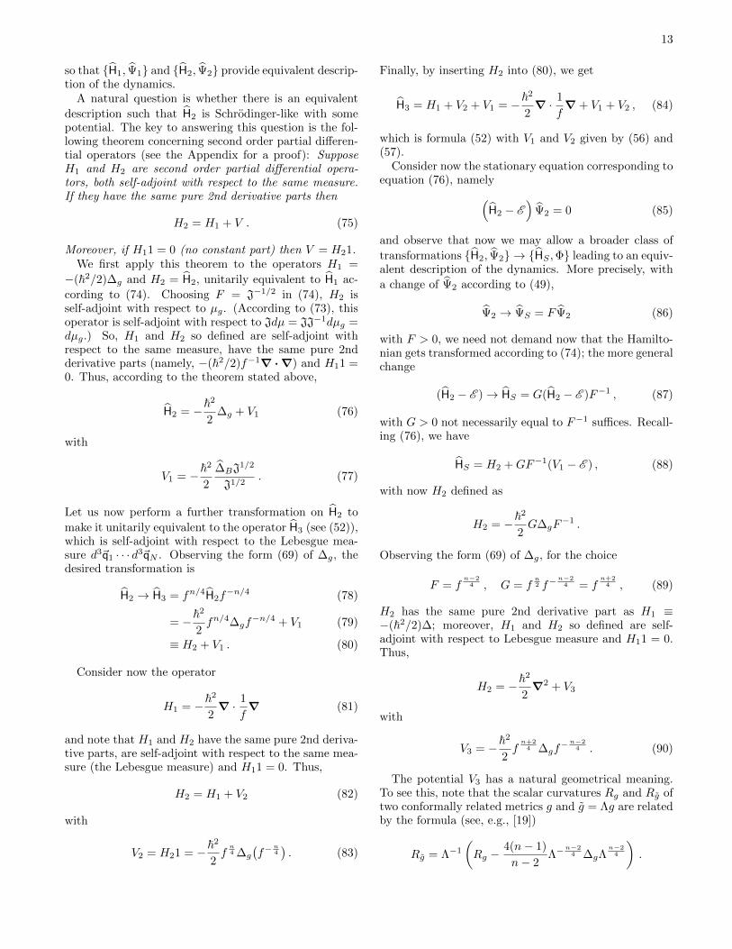
Finally, by inserting H2 into (80), we get

H3 = H1 + V2 + V1 = −~2

2∇ · 1

f∇+ V1 + V2 , (84)

which is formula (52) with V1 and V2 given by (56) and(57).

Consider now the stationary equation corresponding toequation (76), namely(

H2 − E)

Ψ2 = 0 (85)

and observe that now we may allow a broader class of

transformations H2, Ψ2 → HS ,Φ leading to an equiv-alent description of the dynamics. More precisely, with

a change of Ψ2 according to (49),

Ψ2 → ΨS = F Ψ2 (86)

with F > 0, we need not demand now that the Hamilto-nian gets transformed according to (74); the more generalchange

(H2 − E )→ HS = G(H2 − E )F−1 , (87)

with G > 0 not necessarily equal to F−1 suffices. Recall-ing (76), we have

HS = H2 +GF−1(V1 − E ) , (88)

with now H2 defined as

H2 = −~2

2G∆gF

−1 .

Observing the form (69) of ∆g, for the choice

F = fn−24 , G = f

n2 f−

n−24 = f

n+24 , (89)

H2 has the same pure 2nd derivative part as H1 ≡−(~2/2)∆; moreover, H1 and H2 so defined are self-adjoint with respect to Lebesgue measure and H11 = 0.Thus,

H2 = −~2

2∇2 + V3

with

V3 = −~2

2fn+24 ∆gf

−n−24 . (90)

The potential V3 has a natural geometrical meaning.To see this, note that the scalar curvatures Rg and Rg oftwo conformally related metrics g and g = Λg are relatedby the formula (see, e.g., [19])

Rg = Λ−1

(Rg −

4(n− 1)

n− 2Λ−

n−24 ∆gΛ

n−24

).

14

Letting g be the invariant metric on QQQ, g be the Euclideanmetric on QQQ (so that Rg = 0) and Λ = f−1, we obtainthat

Rg =4(n− 1)

n− 2fn−24 ∆gf

−n−24 , (91)

whence

V3 = −~2

2

n− 2

4(n− 1)fRg . (92)

Since GF−1 = f , we conclude that

HS = −~2

2∇2 + f(V1 − E )− ~2

8

n− 2

n− 1fRg , (93)

which coincides with (63) for U given by (64). This com-pletes the proofs of the transitions to the different Hamil-tonians.

Note that while V2 and V3 do not depend on the shapeJacobian J, V1 does. So, to find V1, we have first tofind an explicit formula for J. This will be done in Sect.(VI E) and Sect. (VI F).

D. Remarks on the Bohmian Motion in theVarious Gauges

We have already stated that the usual Bohmian motion

associated with H2 is given by (46), see (23). This is true

also for H1 and H3. To see this, consider a Hamiltonianof the form

H = −h2

2F∇ ·G∇+ U , (94)

with U a potential (multiplication operator), where ∇and ∇· are, respectively, the gradient and the divergencewith respect to a metric with associated volume elementdµ. Then H is self-adjoint with respect to F−1dµ and the

velocity field generated by a solution Ψ of the Schrodingerequation associated with H is

v = ~ ImFG∇Ψ

Ψ. (95)

Thus, in the “1-gauge” for H1 involving ∆B given by (65),

the Bohmian velocity (95) is indeed (46) (with Ψ = Ψ1),since in this gauge ∇ = gradg, ∇· = divg, F = J and

G = J−1. The same velocity arises in the “2-gauge” (76)

(with Ψ = Ψ2), since now F = G = 1 (and ∇ = gradg,∇· = divg, as before), as well as in the “3-gauge” (84)

(with Ψ = Ψ3), since now ∇ = ∇, ∇· = ∇·, the usualdivergence, and F = 1, G = 1/f , so that (95) equals (46)since ∇g = f−1∇. On the other hand, in the “S-gauge”

for HS (the Schrodinger gauge) the Bohmian velocity isgiven by the usual formula (61), which, as already stated,arises from (46) after a time change.

We shall address the status of probability measuresin Bohmian mechanics on shape space and in the variousgauges in Sect. VIII. Here we shall just state some math-ematical facts about the quantum equilibrium measures(Born’s rule) associated with the Bohmian motions in thevarious gauges. These measures are the same in all thefirst three gauges, though they assume different forms.In each gauge, they are the quantum equilibrium mea-sure associated with the solutions of the wave equationin that gauge.

By construction, and more explicitly, since (94) is self-

adjoint with respect to F−1dµ, H1, H2, and H3 are self-adjoint with respect to the measures J−1dµg, dµg, anddq (the Lebesgue measure on QQQ), respectively. Thus,the corresponding quantum equilibrium measures are, re-spectively,

|Ψ1|2J−1dµg

|Ψ2|2dµg|Ψ3|2dq

≡ dµΨ . (96)

The equality of these measures (up to a constant multi-ple) readily follows from the relations between the variousgauges,

Ψ1(q) = Ψ(q) , (97)

Ψ2 = J−1/2Ψ1 , (98)

Ψ3 = fn/4Ψ2 , (99)

and formula (72) for dµg. We finally note that in theSchrodinger gauge, as for the velocity, Born’s probabilitylaw turns out to be the familiar one, namely,

dµΨS = |ΨS |2dq . (100)

Note that in going from the 3-gauge to the S-gauge thereis no change of measure for self-adjointness of the Hamil-

tonian, so that the change Ψ3 → ΨS leads in this case to

a change in measure, µΨS 6= µΨ.

E. Derivation of the Shape Jacobian

We shall now derive formula (65). In order to dothis, we shall compare the Laplace-Beltrami operator∆g on absolute configuration space QQQ with the Laplace-Beltrami operator ∆B on shape space Q = QQQ/G. Thiscomparison would be easy if we could represent ∆g interms of coordinates xi = xH , xV such that the xVcoordinate lines are all inside the G-fibers and the xHcoordinate lines are orthogonal to them and thus yielda horizontal foliation. However, a coordinate system ofthis kind does not exist, not even locally, since the ex-istence of a horizontal foliation of QQQ is precluded by thecurvature of the horizontal connection arising from the

15

rotations (see footnote 5). We shall not elaborate fur-ther on this. Nonetheless a splitting into horizontal andvertical components can be obtained by expressing theLaplace-Beltrami operator in terms of a basis formed bya suitable set of horizontal and vertical vector fields, aswill be explained below.6

First, we express gradient and divergence on a Rie-mannian manifold in terms of a general basis X of vectorfields Xi, i = 1, . . . , n. We replace (66) by(

gradg)i

= gijXj , (101)

where gij = [gij ]−1 with gij = g(Xi,Xj), and replace (67)

with

divg Y =

(1√|g|

Xi√|g|+ ωk ([Xk,Xi])

)Y i , (102)

where |g| = |det(gij)|, ωk is the dual basis in the cotan-gent space, i.e., ωk(Xi) = δki , [ · , · ] is the Lie bracket(or commutator) of vector fields, and Y i are the compo-nents of Y with respect to the basis Xi.7 Accordingly,the Laplace-Beltrami operator (68) becomes

∆g =

(1√|g|

Xi√|g|+ ωk ([Xk,Xi])

)gijXj , (103)

which generalizes the standard formula (68) to an arbi-trary basis.

Second, we specify a basis of vector fields that isadapted to the geometrical structure of absolute config-uration space QQQ as a principal fiber bundle with base Qand fibers isomorphic to the similarity group G, in par-ticular, to the orthogonal decomposition of the tangentspace TqQQQ at any point q of QQQ into horizontal subspaceTqQQQH and vertical subspace TqQQQV and the correspond-ing decomposition TQQQ = TQQQH ⊕ TQQQV of the tangentbundle. In the horizontal subspace we choose as a basisthe horizontal lift of a coordinate basis X = Xα inQ, α = 1, . . . , n − 7. Note that while a lift of the vec-tor field Xα is not unique (as any vector field on QQQ thatprojects down to Xα represents a lift of Xα), there isonly one horizontal lift of Xα which we shall denote by

Xα. These vector fields form the basis XH = Xα ≡ X,α = 1, . . . , n− 7, in the horizontal subspace.

In the vertical subspace we choose a basis formed byvector fields that represent the action of the infinitesimal

6 Moreover, the vertical vector fields that we shall need correspondto the Lie algebra of G, which is noncommutative, and thus donot arise from a coordinate system.

7 Formula (102) is probably in the literature, but we have notsucceeded in finding any reference. It is a straightforward conse-quence, for a manifold with a distinguished volume form (up tosign), of the fact that the divergence of a vector field times thevolume form is the exterior derivative of the contraction of thevector field with the volume form.

generators of the group G on QQQ. More precisely, observethat the action q → g(q) of G on QQQ, g ∈ G, defines, forany given q ∈ QQQ , the map ϕq : G→ QQQ given by ϕq(g) =g(q), and the differential ϕ′q of this map defines a mapfrom Te(G), the tangent space to the identity e of G, toTqQQQ. Since Te(G) is the Lie-algebra g of the group G, theimage under ϕ′q of any element L of g is a tangent vector

at q and, varying q, one obtains the vector field L on QQQassociated with L. In particular, if Lβ , β = 1, . . . 7, arethe generators of g, their images under ϕ′q form the basis

XV = Lβ, β = 1, . . . 7, in the vertical subspace. (Itshould be noted that the vertical vector fields so definedcoincide with the image under ϕ′q of the right invariantvector fields on G; in this regard, recall that the Lie-algebra of the group can be equivalently defined as theLie-algebra of the right —or left — invariant vector fieldson G.)

Third, we rewrite the Laplace-Beltrami operator (103)in terms of the basis X = XH ,XV using the compact(and slightly ambiguous) notation

∆g =1√|g|

XH√|g|gHHXH +

1√|g|

XV√|g|gV V XV

+ ωA ([XA,XA]) gAAX , (104)

where repeated upper and lower indexes H, resp., V ,stands for summation over all elements of XH, resp.,

XV . In the last term the summation is over A = H,V .Note, that no mixed contributions H-V occur, since thevertical and horizontal vector fields are orthogonal and

thus gHV = 0. Consider now ∆gΨ1, the action of ∆g

on an invariant function Ψ1(q) = Ψ(q). Since the secondterm in (104) is purely vertical, it gives no contribution.We rewrite the last term more explicitly, keeping onlythe non zero part of its action on invariant functions, toobtain(

ωH ([XH ,XH ]) + ωV ([XV ,XH ]))gHHXHΨ1 . (105)

The first term in the round brackets gives no contribu-tion, in fact

[XH ,XH ] = [X, X] = [X,X] + Vertical = Vertical ,(106)

where in the last equality we have used the fact that Xis a coordinate basis, and thus its elements commute;moreover, ωH(Vertical) is clearly zero. As for the secondterm, expressing the commutator of the vector fields bymeans of the Lie derivative L,

[XV ,XH ] = LXV XH = 0

by symmetry, i.e., the G-invariance of the vector fields

XH . We conclude that for Ψ1 an invariant function onQQQ, we obtain

∆gΨ1 =1√|g|

XH√|g|gHHXHΨ1 . (107)

16

Fourth, we consider the Laplace-Beltrami operator onshape space acting on ψ = ψ(q),

∆Bψ =1√|gB |

X√|gB |gBBXψ . (108)

Then the action of a lift of ∆B on the invariant functionΨ1 = Ψ1(q) associated with ψ is given by

∆BΨ1 =1√|gB |

XH√|gB |gHHXHΨ1 . (109)

Comparing (109) with (107), we write this as

∆BΨ1 = J1√|g|

XHJ−1√|g|gHHXHΨ1 (110)

with

J =

√|g|√|gB |

. (111)

Fifth (and finally), we consider the operator

O = J divg J−1 gradg ,

with J given by (111), and observe that

J divg J−1Y = J

(1√|g|

Xi√|g|+ ωk ([Xk,Xi])

)J−1Y i

=

(J√|g|

XiJ−1√|g|+ ωk ([Xk,Xi])

)Y i . (112)

Thus OΨ1, with Ψ1 an invariant function, coincides withthe right hand side of (110) (for the same reasons thatled us from (104) to (107)). Therefore O, i.e. (65), is alift of ∆B , with the shape Jacobian J given explicitly byequation (111).

F. Computation of the Shape Jacobian

Our last task is to derive formula (58) from equation(111) for the shape Jacobian J.

First, we observe that in the basis XH ,XV the metricg has the block diagonal decomposition (slightly abusingnotation)

g =

(gV 00 gH

),

where gH can be identified with gB and gV is the restric-tion of g to the vertical vector fields. Since |g| = |gV ||gH |and |gB | = |gH |, it follows from (111) that

J =

√|g|√|gB |

=

√|gV ||gH |√|gB |

=√|gV | , (113)

so that J turns out to be the invariant volume densityin the vertical subspace with respect to fiber volume el-ement corresponding to XV . Moreover, by (6) we havethat

J = f7/2Je , (114)

where Je is the vertical volume density for the mass-weighted Euclidean metric (2) instead of the invariantmetric g involving the conformal factor f . For this wehave

Je(q) = vol(XV )(q) , (115)

the 7-dimensional (Euclidean) volume of the paral-lelepiped in TqQQQV generated by XV , i.e., by the verticaltangent vectors at q obtained by evaluating at q the 7vector fields that generate G.

Second, we may split

XV = (Xtr,Xrs) , (116)

where Xtr refers to the 3 generators of translations andXrs to the 4 generators of rotations and scaling. However,the vector fields Xrs are not in general orthogonal to those

of Xtr. We therefore consider also Xrs = P⊥tr Xrs, the or-thogonal projection of the vectors Xrs into the orthogonalcomplement of the subspace of the tangent space corre-sponding to translations. We thus have that

vol(XV ) = vol(Xtr) · vol(Xrs) (117)

≡ vol(Xtr)Jrs = const Jrs , (118)

since vol(Xtr) is a constant, independent of q (which wemay take to be 1 by letting the translation vectors in

Xtr to be orthonormal). It should be observed that Xrs

consists of the generators of rotations and scalings aboutthe center of mass of the configuration q. To see this,note that if we represent q in center of mass and relativecoordinates q = q − ~qcm, i.e., q = (~qcm, q), then for anyrotation or scaling g, we have that the action of g on q isgiven in these coordinates by g(~qcm, q) = (g(~qcm), g(q)),while for the corresponding action g about the center ofmass, g(~qcm, q) = (~qcm, g(q)).

Third, we may split

Xrs = (Xrot, Xs) (119)

into generators Xrot of rotations about the center of mass

and a generator Xs of scalings about the center of mass.Then we have that

Jrs = vol(Xrs) = vol(Xrot) · vol(Xs) , (120)

since Xs is orthogonal to Xrot.Fourth, we have that

vol(Xs) = L (121)

17

up to a constant, independent of q, where L = L(q) isgiven by equation (9). To see this, note that the effect ofa scaling at q about the center of mass is proportional tothe value of L at q. As for the other volume element in(120), we have

vol(Xrot) =√

detM , (122)

where M is the tensor of inertia of the configuration qabout the center of mass, whose matrix elements withrespect to an orthogonal cartesian system x,y,z are givenby equation (12). This formula for the volume element ispresumably standard. A way to see how it comes aboutis the following.

To simplify the notations, let us drop “tildas” and“rot” and stipulate that in this paragraph (Xi), i =x, y, z, denotes a basis for the generators of rotationsabout the center of mass ~qcm (x, y, z refer to any or-thogonal frame with origin in the center of mass). Then

the volume element in (122) is given by√

detA, whereA is the matrix with entries Aij = ge (Xi,Xj). Forq = q − ~qcm a configuration relative to the center ofmass, let q = (~q1, . . . , ~qN ). Observe that a generator cor-responding to the action of a rotation on configurationsis of the form XΩ(q) = (Ω×~q1, . . . ,Ω×~qN ), where Ω is a3-dimensional vector of components Ωi (with respect tothe xyz frame). Thus the 3-dimensional Lie algebra cor-responds naturally to the 3-dimensional vectors Ω, withΩi being the coordinates of a general element XΩ of theLie algebra with respect to the basis (Xi). A vector Ωcorresponds to a general instantaneous rotational motion.Consider the kinetic energy

K =1

2ge(XΩ,XΩ) (123)

for such a motion. On the one hand, it is known to begiven by

K =1

2MijΩ

iΩj , (124)

where M = Mij is the moment of inertia tensor. Onthe other hand, expanding the right hand side of (123) byexpressing XΩ =

∑i ΩiXi in the basis (Xi), one obtains

ge(XΩ,XΩ) = ge (Xi,Xj) ΩiΩj = AijΩiΩj .

Thus equating the right hand sides of (123) and (124),one sees that the matrix A is indeed the tensor of inertiaM, whence equation (122).

Fifth (and finally), substituting in (114) the formula

for Je given by (115), with vol(XV ) = Jrs, and using

formulas (120),(121), and (122) for Jrs, we have that

J = Lf7/2√

detM ,

which is formula (58) for the shape Jacobian.

G. More Gauge Freedom

As we have already stressed, the lift to QQQ of theLaplace-Beltrami operator ∆B on Q is by no meansunique. The “canonical lift” (65), with J given by equa-tion (58), is very natural, but other choices are possible.This lack of uniqueness increases the gauge freedom wehave in defining the Schrodinger gauge. In particular, wemay use this freedom to define a shape Jacobian that isan invariant function on QQQ, i.e., a function of the config-uration q which depends only on its shape.

Note that J is not invariant: f7/2 scales like L−7 and√detM like L3. We thus have that

J = L−3JB , (125)

where

JB = f7/21

√detM1 (126)

is invariant. Here the subscript 1 indicates the quantitieshave to be evaluated, not at q, but at q1, the configura-tion with L = 1 obtained by rescaling q.

To define a lift ∆B of ∆B , we could as well have usedthe invariant

JB = L3J = L4f7/2√

detM (127)

instead of J. This would have in no way affected theresults and the arguments in Sect. VI C and Sect. VI E,though it would yield somewhat different potentials Vand U in (52) and (63), respectively.

H. The Canonical Conformal Factor

Instead of computing JB for a given f , we might read(127) the other way round, and ask what is the conformalfactor that gives rise to the simplest JB . The simplestpossibility is JB = 1 and this is associated with f(q) ≡fc(q) given by equation (13), i.e.,

f(q) = fc(q) ≡ L−87 (detM)−

17 ,

the canonical conformal factor. Note that replacing J in(56) with JB = 1 gives V1 = 0 so that the potential inthe Hamiltonian (52) is V = V2, with the form (57) ofV2 unaffected. (Of course, one needs to evaluate it forf = fc.) Similarly, the potential U in (64) becomes

U = −fcE −~2

8

n− 2

n− 1fcRgc , (128)

where Rgc (cf. (91)) is now the scalar curvature of themetric g = gc associated with fc.

18

VII. SUBSYSTEMS

A. Conditional Wave Functions

In physics we are usually concerned not with the entireuniverse but with subsystems of the universe, for exam-ple with a hydrogen atom or a pair of entangled photons.The quantum mechanical treatment of such systems in-volves the quantum state of that system, often given byits wave function—not the wave function of the universe.Bohmian mechanics provides a precise formulation andunderstanding of this notion in terms of the conditionalwave function [11]

ψ(x) = Ψ(x, Y ) , (129)

where Ψ = Ψ(q) = Ψ(x, y) is the wave function of theuniverse, with x and y the generic variables for the config-urations of the system and its environment, respectively,and where Y is the actual configuration of the environ-ment. The conditional wave function of a Bohmian sys-tem behaves exactly as one would expect the wave func-tion of a system to behave, with respect to both dynamicsand statistics. It is natural to ask how and whether theconditional wave function can be defined for Bohmianmechanics on shape space.

For this the following problem arises. There is no nat-ural product structure

Q = Qsys × Qenv

for shape space: Here the system is a collection of (la-belled) particles with its own shape space Qsys = X, theset of possible shapes X of the system, and the environ-ment consists of the rest of the particles of the universe,with shape space Qenv = Y = Qenv = Y , with Y theshape associated with the particles (labels) of the envi-ronment. The crucial fact is that it is not true that

Q = X ×Y.

X and Y don’t involve sufficient information to determinethe complete shape Q. What is missing is the spatialrelationship between these shapes.

Nonetheless we have that Q can be identified with

XY ×y Y = (X,Y )|Y ∈ Qenv, X ∈ QY ,

where

QY = Q ∈ Q|Qenv = Y .

We may then define the conditional wave function forthe subsystem, for Y ∈ Qenv and universal wave functionΨ, by

ψ(x) = Ψ(x, Y ), x ∈ QY . (130)

This looks like the usual conditional wave function, but itis important to bear in mind that, unlike with the usual

conditional wave function, here x represents the shapeof the universe for a fixed Y and there are no obviousnatural coordinates to efficiently describe it.

To obtain such a thing the notion of a frame might beuseful: Given Y ∈ Qenv, a frame Y is a choice of pointin the fiber over Y in the absolute configuration space ofthe environment. (Y corresponds roughly to the usualnotion of frame of reference.)

Given Y and a frame Y , we obtain natural coordinatesfor QY : Given X ∈ QY there is a unique X ∈ R3M

(with M the number of particles of the subsystem, whichwe shall assume from here on is such that the numberof particles in the environment N −M ≥ 3) such that(X,Y ) is in the fiber above X ∈ QY . The map X 7→Xis a one-to-one correspondence between QY and R3M .

Given the frame Y , we may represent the conditionalwave function by

ψ(x) = ψ(x), (131)

where x corresponds to x. In other words,

ψ(x) = Ψ(x,Y ), (132)

with Ψ the lift of Ψ to absolute configuration space, Ya lift of Y , x the lift of x in the frame Y , and the “hat”

refers to any of the gauge equivalent representations Ψ1,

Ψ2, Ψ3 (and presumably ΨS) of the universal wave func-tion that we have described in Sect. VI C. Thus, the abso-lute configuration space level conditional wave functions

ψ1, ψ2 and ψ3 (and ψS) are at the same time differentrepresentations of the shape space conditional wave func-

tion. Moreover, the ψs obtained using different framesare in an appropriate sense equivalent.

This conditional wave function ψ behaves like the wavefunction of the subsystem, both with respect to the dy-namics of configurations, via the guiding equation, andwith respect to probabilities for the subsystem, via whathas been called the fundamental conditional probabilityformula [11]. With regard to the dynamics, this is clearfrom the form of the dynamics on absolute configurationspace. The latter, while true, is not at all so clear. Thatit is so follows from the analysis in Sect. VIII.

B. Subsystems and the Role of Projectivity

The time-parameter corresponding to the use of thedenominator in footnote 3 has the nice feature that thedynamics using that time-parameter depends on fewerdetails of the wave function than would be the case if thedenominator were deleted: with the denominator the dy-namics depends only on the ray of ψ, with ψ and cψ yield-ing the same dynamics for any constant c 6= 0. This hasa particularly nice implication for the behavior of subsys-tems. With this choice of time-parameter the dynamicsfor a subsystem will often not depend upon the config-uration of its environment, with the subsystem evolving

19

according to an autonomous evolution involving only theconfiguration and the (conditional) wave function of thesubsystem itself [11]. This would happen when the sub-system is suitably decoupled from its environment, forexample for a product wave function when there is nointeraction between system and environment. Withoutthe denominator this would not be true, and there wouldappear to be an additional nonlocal dependence of thebehavior of a subsystem on that of its environment thatwould not be present with a time-parameter associatedwith the use of the usual denominator.

C. The Emergence of Metrical Time

By metrical time we refer to any objective physicalcoordination of the configurations along a geometricalpath in a configuration space with the points of a one-dimensional continuum: a (continuous) mapping fromthe continuum onto the path. The continuum is usu-ally represented by the real numbers, but it need notbe. However, it should be physically distinct from theparticular continuum that is the path itself.

Understood in this way, metrical time does not exist,from the relational point of view, for the universe as awhole. However, for subsystems of the universe metricaltime naturally emerges: the continuum with which thegeometrical path corresponding to the evolution of thesubsystem is coordinated can be taken to be the path ofits environment, with the obvious mapping between thepaths.

VIII. PROBABILITY

A. Bohmian Mechanics and Probability

In Bohmian mechanics, for a non-relativistic systemof particles, the configuration of a system is regardedas random, with randomness corresponding to the quan-tum equilibrium distribution µψ given by |ψ|2dq. Whatthis actually means, in a deterministic theory such asBohmian mechanics, is a delicate matter, involving along story [11] with details and distinctions that weshall ignore here. However a crucial ingredient for thatanalysis—for an understanding of the origin of quan-tum randomness in a universe governed by Bohmianmechanics—is the fundamental conditional probabilityformula for the conditional distribution of the configu-ration Xt of a system at time t given that of its environ-ment Yt at that time:

PΨ0(Xt ∈ dx |Yt) = |ψt(x)|2dx, (133)

where Ψ0 is the initial wave function of the universe andPΨ0 is the probability distribution on trajectories aris-ing from the Bohmian dynamics with an initial quantumequilibrium distribution, and ψt is the (normalized) con-ditional wave function (129) of the system at time t.

A crucial ingredient in proving (133) is equivariance[11]: if at any time the system configuration is randomlydistributed according to |Ψ0|2, then at any other time tit will be distributed according to |Ψt|2. Equivarianceis an immediate consequence of the continuity equationarising from the Schrodinger equation:

∂ρΨ

∂t+ div JΨ = 0 , (134)

with ρΨ = |Ψ|2, the quantum equilibrium distribution,and

JΨ = ρΨvΨ , (135)

the quantum probability current, where vΨ is theBohmian velocity in the right hand side of (22),

vΨ = ~ Im∇Ψ

Ψ(136)

(as usual here, the masses are absorbed in the gradient).More generally, for Bohmian mechanics on a Rieman-

nian manifold with metric g, the quantum equilibriumdistribution µΨ is given by |Ψ|2dµg. In terms of any co-ordinate system x = (x1, . . . , xn), we have that

dµg =√|g|dx, (137)

where dx = dx1 · · · dxn and g = gij = g(Xi,Xj), withXi = ∂/∂xi.

Moreover, as already indicated several times, theBohmian velocity on a Riemannian manifold is still givenby (136) with ∇ = ∇g, the gradient with respect tothe metric g. Furthermore, letting ρΨ be the densityof µΨ with respect to µg, i.e., ρΨ = |Ψ|2, the current ismost conveniently represented as a density with respectto µg as in (135); in this representation the continuityequation (134) holds for div = divg, the divergence withrespect to g. So, all the Bohmian structure, includingthe quantum equilibrium measure, transfers straightfor-wardly from the familar Euclidean setting to a generalRiemannian manifold.

B. The Problem of Non-Normalizable Measures

Note that since it is translation and scaling invariant,the wave function in the Schrodinger gauge or in any ofthe gauges discussed in Sect.VI B) are not normalizable.

In other words, µΨS and µΨ given by (100) and (96),respectively, are non-normalizable. However, since thenon-normalizability arises from unobservable (and, froma shape space point of view, unphysical) differences anddimensions it should somehow not be a problem.

Nonetheless, the real question is how the empirical dis-tributions arising from the fundamental shape space levelcompare with those coming from the physics in a gauge.While the different gauges, such as the Schrodinger

20

gauge, correspond to theories that, we argued, are empir-ically equivalent to the fundamental shape space theory,that was only in purely dynamical terms. We have notyet addressed the possible differences in empirical distri-butions that may arise. We would like to see that theydon’t.

There are several considerations that suggest that thenon-normalizability should not be a genuine problem:

1) As just mentioned, the non-normalizability arisesonly from non-observable dimensions, suggestingthat it should be physically irrelevant.

2) It is the universal wave function Ψ (in any of thegauges) that is not normalizable. But the universalwave function is rarely used in practice. In quan-tum mechanics we usually deal, not with the entireuniverse, but with small subsystems of the universe.The wave functions with which we usually deal arethus conditional wave functions, and there seemsto be no reason why these should fail to be normal-izable.

3) In statistical mechanics the Lebesgue measureon the phase space for a gas in a box is non-normalizable. Why is this not a problem? It isbecause the energy is a constant of the motion,and the restriction of the Lebesgue measure to theenergy surface is normalizable (for suitable poten-tials). Similarly here, with Bohmian mechanics inthe Schrodinger gauge, or in any of the gauges onabsolute configuration space, the center of massand the moment of inertia about the origin, orabout the center of mass, are constants of the mo-tion. Thus, it would seem that the appropriate

measure that we should be considering here is µΨΓ ,

the conditional distribution for µΨ given Γ, the one

given by |Ψ|2 on a surface Γ of constant center ofmass and moment of inertia about the origin, andnot on the entire absolute configuration space, andthis is presumably normalizable. Moreover, all suchprobability distributions, for different choices of Γ,are physically equivalent, since they correspond tothe same probability distribution on shape space.

The probability distributions described in 3), whilethey seem to correspond to the appropriate measures onshape space, appear to be entirely inappropriate inso-far as the fundamental conditional probability formulais concerned. For example, for a single-particle systemthe configuration of that system would be completely de-termined by the configuration of its environment, ratherthan being randomly distributed according to the quan-tum equilibrium distribution. What gives?

C. The Fundamental Conditional ProbabilityFormula for Evolving Wave Functions

In order to answer the last question, as well as to ob-tain a sharp resolution of the non-normalizability issueand an understanding of how to carry out the usual quan-tum equilibrium analysis [11] yielding the Born rule, thefollowing observation is crucial: The conditional distri-

bution, arising from µΨ, of the configuration of a systemgiven its environment in absolute configuration space isunphysical, and is thus not relevant to an appropriatequantum equilibrium analysis. That is because (from theshape space point of view) the absolute configuration ofthe environment is unphysical. What is physical, andwhat we should be conditioning on, is the shape of theenvironment. And when we condition on this, the resultwill be given in terms of the conditional wave function

ψ (131).In fact, on the fundamental level, with respect to

the quantum equilibrium distribution on shape space,dµΨ

B = |Ψ|2dµB (where dµB ≡ dµgB ), the conditionaldistribution of the configuration of a system (i.e., of theconfiguration of the universe, see (130)) given the shapeof its environment is perhaps most naturally expressedon the absolute level, via the use of a frame and of the

corresponding conditional wave function ψ in any one ofthe first three gauges—for example, the conditional wavefunction in the first gauge we considered, namely thestraightforward lift (45)—using the frame Y rather thanthe shape Y . And since the quantum equilibrium distri-bution for this conditional wave function represents thecorresponding conditional distribution on shape space (aswe shall argue below), it follows that the conditional wavefunction on absolute configuration space is normalizable.

That this is in fact so, i.e., that the lift to absoluteconfiguration space of the fundamental conditional prob-ability formula on shape space is given by the Born rulefor the conditional wave function on absolute configura-tion space, can be seen as follows:

• Unlike marginal distributions, conditional mea-sures are well defined, up to a constant multiple,even for a non-normalizable measure µ.

• Suppose we condition on something, for example,the environment Y of a subsystem, correspondingto a leaf ΓE of a foliation E (e.g., into the levelsets of the random variable Y ). We would obtainthe same result if we had first conditioned on aleaf ΓF , ΓE ⊂ ΓF , of a coarser foliation8 F ⊂ E ,obtaining the conditional measure µΓF

, and then,with respect to µΓF

, conditioned on ΓE .

8 identifying F and E with the σ-algebras they generate, consist-ing of the measurable sets that are unions of the leaves of therespective foliations

21

• For µ = µΨ, the (non-normalizable) quantumequilibrium distribution on absolute configurationspace, we can choose F so that the measures µΓF

all correspond to the quantum equilibrium distribu-tion on shape space, and E so that it correspondsto the shape of the environment.

• If this can indeed be done we obtain our desiredresult.

In more detail, fix now the subsystem, and let E cor-respond to the configuration Y of its environment. Fmust be chosen so that the following is true: Each leafof F must provide a representation of shape space as ameasure space. Not only must there be a smooth bijec-tion between shape space and each leaf of F , but underthis bijection we must have that each of the measuresµΓF

corresponds to µΨB . Moreover, we must also have

that (i) the leaf of F to which an absolute configurationbelongs is determined by the configuration of its envi-ronment, i.e., F ⊂ E , and that (ii) different leaves of Ebelonging to the same leaf of F correspond to environ-mental configurations with different shapes, so that withrespect to the bijection, the configuration of the environ-ment corresponds to its shape.

Such an F can be generated from a cross-section ofthe absolute configuration space of the environment re-garded as a bundle over its shape space. Such a cross-section naturally induces a cross-section in the universalabsolute configuration space regarded as a bundle overshape space (since for any shape there is a unique ab-solute configuration compatible with the environmentalcross-section). The cross-section so obtained provides asingle leaf Σ1 of F ; the other leaves of F are obtainedby the application of the symmetry group G to Σ1. Inthis way, absolute configuration space can be identifiedwith G × Σ1, with F corresponding to G, i.e., havingleaves Σg = gΣ1.

Note that with this F we have, essentially by construc-tion, that the shape of the environment corresponds, oneach leaf of F , to its absolute configuration. Note alsothat this would not be true for the foliation correspond-ing to the (quotient under rotations of the) surfaces Γdescribed in 3) of Sect. VIII B, for which a single shapeof the environment would correspond to many differentabsolute environmental configurations on each leaf (evenafter rotations have been factored out).

We now check that for this F the conditional measuresµΓF

correspond to the quantum equilibrium distributionon shape space. For this we will use the following generalformula for the Riemannian volume element µg in termsof a general basis of vector fields Xi:

dµg =√|g| dω1 · · · dωn ,

where |g| is defined below (102). This formula is simi-lar to (137) for the case when the vector fields are co-ordinate vector fields, but with dx1 . . . dxn replaced bydω1 · · · dωn, the volume element arising from the n-form

dω1 ∧ · · · ∧ dωn, where ω1, . . . , ωn is the basis of 1-formsdual to the basis X1, . . . ,Xn of vector fields, see Sect.VI E.

For the basis of vector fields X = (XV ,XH) describedthere, we obtain that

dµg =√|g| dωV dωH =

√|gV |

√|gH | dωV dωH ,

where dωV is the volume element arising from XV , avolume element on the fibers of absolute configurationspace, and dωH corresponds to the volume element onshape space arising from the coordinate system involvedin the definition of XH .

Since√|gH | dωH corresponds to

√|gB |dx = dµB ,

where dx is the coordinate measure on shape spacefor these coordinates, we have that dµg corresponds to√|gV | dωV dµB . Moreover, dωV is, up to a constant fac-

tor, the image of the right Haar measure µG on G. Wethus have, using the representation G × Σ1 for absoluteconfiguration space, that

dµg = JdµGdµ1B ,

where J is given in (113) and µ1B is the image of µB on

Σ1.Now since ∆B , see Sect. VI B, is self-adjoint, not with

respect to dµg, but with respect to J−1dµg = dµGdµ1B ,

we have that, for ∆B , and any wave function Ψ on shapespace, the quantum equilibrium distribution µΨ is givenby

dµΨ = |Ψ|2dµGdµ1B .

Thus, for µΨ, the conditional probability distribution

given G is |Ψ|2dµ1B , i.e., the image of µΨ

B , just as wewanted.

Finally, as we indicated earlier in Sect. VI D, as weproceed through the first three gauges, each involvingits own wave function and measure for self-adjointness,the transformations connecting the gauges have been sodefined as to leave invariant the corresponding quantum

equilibrium distributions µΨ. For each gauge, we are infact dealing with the same measure on absolute config-uration space, and hence the same conditional measuregiven a leaf ΓF of the foliation F and the same condi-tional measure given a leaf ΓE of the foliation E . Thus ineach gauge, the conditional distribution of the quantumequilibrium measure given the configuration of the envi-ronment yields, in fact, the conditional distribution onshape space given the shape of the environment, whichis what we wanted to establish.

In summary, we have obtained that the conditionaldistribution of the configuration X of a system given theshape Y of its environment is given by

µΨB(X ∈ dx |Y ) = µΨ(X ∈ dx|Y ) . (138)

As a consequence, we have (from equivariance) the fun-damental conditional probability formula on shape space,

22

for the conditional distribution of the configuration Xt ofa system at time t given the shape Yt of its environmentat that time.

Fundamental conditional probability formula onshape space:

PΨ0(Xt ∈ dx |Yt = Y ) = µΨt(X ∈ dx|Y ) , (139)

where Ψ0 is the initial universal wave function on shapespace (at t = 0), Y is a lift of Y , x the lift of x inthe frame Y , Ψt is the universal wave function at time t,

with µΨt the non-normalizable quantum equilibrium mea-sure on absolute configuration space—the lift (96) of thequantum equilibrium distribution µΨ

B on shape space.

In the 3-gauge this can be written in a more familiarand explicit manner:

PΨ0(Xt ∈ dx |Yt = Y ) = |ψ3,t(x)|2dx (140)

= C|Ψ3,t(x,Y )|2dx , (141)

where ψ3,t is the (normalized) conditional wave functionin the 3-gauge in the frame Y and C is a normalizationconstant.

D. The Physical Significance of the ConditionalDistribution for Stationary Wave Functions

However, what has just been said is not quite right forthe Schrodinger gauge corresponding to the transitionfrom (52) to (63). As already indicated at the end ofSect. VI D, this involves no change of measure for self-

adjointness, so that µΨS 6= µΨ. This might seem bad.

On the other hand, the change in µΨ is precisely the oneimplied by the random time change arising from replacingf−1∇ by ∇, as described above (61). This seems sort ofgood. But one should be puzzled by the fact that thisrandom time change leads to a change in the measure

µΨ, which would seem to have some physical significance.But how could it, since the random time change has nophysical significance?

So there are several questions here that need to be un-derstood better: (i) What is genuinely physically signifi-

cant in µΨ? (ii) How does that resolve the apparent prob-lem that in the Schrodinger gauge we are dealing with a

µΨS that is incompatible with µΨB and thus apparently

one that would yield an incompatible fundamental con-ditional probability formula in the Schrodinger gauge?

A crucial ingredient in an answer to these questions is

the claim that it is not exactly µΨ, resp. µΨS , that isphysically relevant. Rather what is physically relevant is

the associated current J Ψ = ρΨvΨ, resp. J ΨS = ρΨSvΨS ,

where ρΨ ∝ ρΨ3 , resp. ρΨS , is the density of µΨ, resp.

µΨS , with respect to the Lebesgue measure. The cur-rent is invariant under all the transitions, either because

both factors are or because the changes in the factorscompensate each other.

Now why should the current be what is physically rele-vant? Because it yields the same crossing probabilities forhypersurfaces—that either yield the probability distribu-tion on geometrical paths in configuration space, or theprobability distribution associated with the return mapfor Poincare sections corresponding to physical situationson which we wish to condition. Concerning the former,this could correspond to conditioning on the value of asuitable clock variable, for which the corresponding con-ditional wave functions have more familiar quantum evo-lutions, so that first conditioning on such a clock variablewould put us back in a more familiar situation to whichthe argument described above would apply.

Be that as it may, let’s return to the question of why

the change in the measure µΨ (µΨS = f−1µΨ) arisingfrom the random time change has no physical signifi-cance. We have argued that the main physical relevance

of µΨ resides in the implied conditional distribution ofa subsystem given its environment. Suppose f dependsonly upon the environment. In this case, the change inmeasure associated with f produces no change in the cor-responding conditional distribution.9 And it seems likelythat for reasonable choices of f , such as those given inSect.II D above, it will approximately be a function ofthe environment, with negligible error for subsystems ofreasonable size, much smaller than that of the universe.

But even if this is so, the question remains as to exactlywhat of physical significance this conditional distributionrepresents. After all, the transition to the Schrodingergauge required relational time, but if we take relationaltime seriously, what is physical is not the configurationQt of the universe at some time t, but the geometricalpath of the full history of the configuration, with no spe-cial association of the configurations along a path withtimes. In this (more physical) framework, the conditionaldistribution of the configuration Xt of a subsystem giventhe configuration Yt of its environment is not meaningful.

9 Letting x and y be the configuration variables of system andenvironment, respectively, note that if f does not depend on x,the kinetic energy term in the Hamiltonian (84) will be

−~2

2

[1

f(∇2)x + (∇ ·

1

f∇)y

],

where ∇ and ∇· are the mass-weighted Euclidean gradient anddivergence and the subscripts refer to their restrictions to the x-variables and the y-variables, respectively. Accordingly, when-ever the system is decoupled from its environment, its condi-tional wave function ψ3(x) = Ψ3(x,Y ) will evolve (after suit-able rescaling) according to the standard Schrodinger Hamilto-nian with masses f(Y )mα, α = 1, . . .M , where Y is the actualconfiguration of the environment. Thus, in this case, the effectof the environment on the system corresponds just to a (possiblytime-dependent) rescaling of the masses. Then it turns out thatthe 3-gauge is more similar to the Schrodinger gauge than onemay have expected.

23

What is meaningful is (i) a probability distribution Pon the space P of (geometrical, i.e. unparametrized)paths (determined by the current, for example by usinga cross-section, as we shall explain in Sect. VIII E) and(ii) the conditional distribution relative to P of the con-figuration XY of the subsystem when the path γ ∈P hasenvironmental configuration Y, given that the path passesthrough a configuration with environment Y , Y ∈ γ.10

We assume here that there is at most one such configu-ration for (any) Y .11

E. The Association Between Measures on PathSpace and on Configuration Space

We shall now elaborate on the relations between mea-sures on a configuration space Q and measures on a setP of (smooth) paths on Q forming a one-dimensionalfoliation of Q. First, let us fix the notations: we shalldenote by γ a path in P, by q a point in Q and by γ(q)the path passing through q.

We introduce the notion of time function on Q: asmooth real-valued function τ = τ(q), q ∈ Q, whichis monotonic (and extends from −∞ to +∞) on eachpath γ ∈P. The latter is related to, but different from,the notion of dynamics on Q (in the sense of the theoryof dynamical systems): a one parameter family of (in-vertible and smooth) maps T = Ts on Q, with time svarying on the reals. Clearly, a time function τ generatesa dynamics T = T τ such that

τ(Ts(q)) = τ(q) + s . (142)

Let τ be a time function and denote by dτγ(q) theinfinitesimal increment of time (with respect to the timefunction τ) along a path γ passing through q. Considerthe function on path space (random variable) giving thetime spent in the region A ⊂ Q by the path, relative tothe time function τ :

τ(A) = τγ(A) =

∫A

dτγ(q) .

Let

E (τ(A)) =

∫P

τγ(A)P(dγ) (143)

10 This seems to involve a new sort of conditional probability anal-ogous to the so-called Palm measure. In particular, it does notappear to be a special case of the conditional distribution rela-tive to a Σ-algebra or a foliation or given the value of anotherrandom variable. That is because any path will involve configu-rations with many different environments Y.

11 When Ψt is time-dependent, it is natural to suppose that thetime-parameter t has physical significance via the changes in typ-ical configurations arising from changes in µΨt . In this situation,treating time as if it were physical and observable seems to be areasonable approximation. In any case, this is an approximationwe almost always make, and it seems to often work quite well.

be the expected value with respect to P of τ(A) (i.e., theexpected time spent by the path in A) relative to the timefunction τ . We say that µ is associated with P and τ if

µ(A) = E (τ(A)) . (144)

The measure µ can also be described as follows. Wemay identify configuration space Q with P × R by as-sociating any configuration q with the path to which itbelongs and the time along the path:

q 7→ (γ(q), τ(q)) .

Under this identification µ is the product of P and theLebesgue measure, dµ = dP dt.

If µ is associated with P and τ , then we have that Parises from conditioning µ on τ ,

P(S) = µ(S | τ = t) (145)

where S is a set of path and S = q ∈ Q |γ(q) ∈ S. Notethat the right hand side of (145) does not depend on t.(It follows from (142) and (143) that µ is stationary withrespect to the dynamics Ts generated by τ according to(142).) Conversely, when µ, P, and τ are related as in(145), µ is associated with P and τ .

Suppose now that µ is stationary for a dynamics Tfor which τ is a time function,12 i.e., such that (142) issatisfied. Let P be a measure on P, the path space ofthe dynamics. Then the following are equivalent:

P(S) = µ (q ∈ Q |0 ≤ τ(q) ≤ 1 and γ(q) ∈ S)(146a)

P(S) = µ(S | τ = t) . (146b)

When µ and P are associated in this way then say thatP is generated by µ and T , and if this is so, then µ isassociated with P and τ . In particular, if τ is a timefunction for any Bohmian dynamics with stationary Ψ (orµΨ) then µΨ is associated with PΨ and τ , where PΨ is themeasure generated by µΨ and the Bohmian dynamics.

Furthermore, if the dynamics T is given by a vectorfield v, P is generated by µ and T if and only if

P(S) =

∫ΓS

J · dσ , (147)

where J = J(µ, T ) is the current associated with the dy-namics. Here ΓS = Γ∩ S, where Γ is any cross section ofthe foliation P, for example the level surface τ(q) = t.If µ is absolutely continuous with density ρ (with respectto the coordinate measure in some coordinate system),then J = vρ (with v represented in that coordinate sys-tem) and the surface integral above is given by the usualformula.

12 Note that, as a consequence of Poincare recurrence, in generalthere might be no time function associated with a dynamics T .However, if one does exist, it cannot be unique, because it woulddepend on the choice of an initial cross section.

24

F. A Conditional Probability Formula for PathSpace Measures

In this section and the next we consider a fixed system(and its environment), with configuration Q = (X,Y ).We also fix the configuration Y of the environment. Weprove a crucial fact for establishing in Sect. VIII G thefundamental conditional probability formula for station-ary wave functions, a general fact that we call the pathspace conditional probability formula.

In this formula we condition on the path space eventY ∈ γ ⊂ P that the path γ contains a configurationwith environmental configuration Y , i.e., on the set ofpaths γ that pass through a configuration with environ-ment Y . And in this formula we are interested in theconditional distribution of XY , the configuration of thesystem when the path passes through the configurationwith environment Y , a function (random variable) on thesubset Y ∈ γ of path space P.

Path space conditional probability formula: LetP be a measure on the path space P. Suppose µ is themeasure on the corresponding configuration space Q as-sociated with P and a time function τ that depends onlyupon the configuration Y of the environment. Then

P(XY ∈ dx|Y ∈ γ) = µ(X ∈ dx|Y ) . (148)

This follows more or less as before (see the second bul-let of Sect. VIII C) with E , as before, corresponding tothe configuration of the environment and now F cor-responding to the foliation given by the time function.In more detail, since the time function depends only onY , E ⊂ F . Under the natural identification of pathspace with any leaf of F , the event XY ∈ dx becomesX ∈ dx, the event Y ∈ γ becomes the event thatthe environment has configuration Y , and by (145) P be-comes the appropriate conditional measure.

G. The Fundamental Conditional ProbabilityFormula for Stationary Wave Functions

We assume now that there exists a time function forthe Bohmian dynamics that depends only on the config-uration of the environment, an assumption that we callthe existence of clock variables for the Bohmian dynam-ics. Under this assumption the conditional distributionPΨ(XY ∈ dx|Y ∈ γ) is given by the usual Born’s rule onabsolute configuration space.

Fundamental conditional probability formula forstationary wave functions: Suppose that there existsa clock variable for the Bohmian dynamics generated bya stationary wave function Ψ on shape space, as well asone for the Bohmian dynamics in the Schrodinger gauge.Then

PΨ(XY ∈ dx|Y ∈ γ) = µΨ(X ∈ dx|Y ) (149)

in any of the first three gauges,13 or

PΨ(XY ∈ dx|Y ∈ γ) = C|ΨS(x,Y )|2dx (150)

in the Schrodinger gauge (as before, C is a normalizationconstant) where Y is a lift of Y and x is the lift of x

in the frame Y . Here Ψ and ΨS are the lifts of Ψ inany of the first three gauges or in the Schrodinger gauge,respectively.

This is a consequence of the path space probabilityformula (148). Applying it to the Bohmian dynamics (i)on shape space, (ii) in the first three gauges, and (iii) inthe Schrodinger gauge, we obtain the following:

PΨ(XY ∈ dx|Y ∈ γ) = µΨB(X ∈ dx|Y ) (151)

PΨ(XY ∈ dx|Y ∈ γ) = µΨ(X ∈ dx|Y ) (152)

PΨS (XY ∈ dx|Y ∈ γ) = µΨS (X ∈ dx|Y ) , (153)

given the existence of clock variables for the Bohmiandynamics. Here γ is a path for the dynamics on absoluteconfiguration space.

By (138) the right hand sides of (151) and (152) agreewhen x and Y are appropriate lifts of x and Y , so that

(149) follows. Since the currents J associated with µΨ

and µΨS arising from their respective dynamics are the

same, it follows that PΨ = PΨS , so that the right handsides of (152) and (153) are also the same. Thus (150)follows as well.

H. Typicality

As a partial summary, we find that on the absoluteconfiguration space level the dynamics and the probabil-ities for subsystems should be of the usual form. While itis true that on the universal level the connection between|Ψ|2 and probability, or, more precisely, typicality, wouldbe broken, this would not be visible in any of the familiarevery day applications of quantum mechanics, which areconcerned only with subsystems and not with the entireuniverse.

In particular the patterns described by the quantumequilibrium hypothesis will be typical with respect to ameasure, not on absolute configuration space, but onshape space, on the fundamental level, which is fine.There is a widespread misconception with respect toBohmian mechanics that |Ψ|2 for the universe and |ψ|2for subsystems play, physically and conceptually, similarroles. They do not, since the role of |Ψ|2 is typicality

13 These formulas, for the different gauges, may appear to be incom-patible. But for the condition relating Ψ and the time-parameterto hold for both the Schrodinger gauge and any other gauge, thecondition on f mentioned above would presumably have to besatisfied, in which case the formulas would agree.

25

while that of |ψ|2 is probability. If this distinction is toosubtle, the fact that, from a relational perspective, theseobjects live on entirely different levels of description, |Ψ|2on the fundamental level, i.e., on shape space, and |ψ|2on absolute configuration space, might make it easier toappreciate how very different they are.

IX. OUTLOOK

The basic problem in cosmology is to determine whichlaws govern the universe as a whole. The traditionalapproach is that of building a story about the universestarting from the physical laws operating at small scales,such as the Standard Model of particle physics, and incor-porating them within a theory containing a now missingquantum theory of gravity. However, the relational pointof view suggests that there is something basically wrongin treating the universe as a whole as a mere combinationof the systems that compose it, say galaxies or cluster ofgalaxies. We elaborate.

Shape space physics is genuinely holistic, and suggeststhe holistic character of quantum physics associated withentanglement and quantum nonlocality. To appreciatethis point, note that for relational space the state of theuniverse at a particular location is not, in and of itself,meaningful. In that sense, for shape space physics, thereare no local beables, so that locality itself can’t easily bemeaningfully formulated. Similarly one can’t meaning-fully consider the behavior of individual particles with-out reference to other particles, since there is no absolutespace in which an individual particle could be regardedas moving. And even for a pair of particles, to speakmeaningfully of the distance between them, a third par-ticle would be required, to establish a scale of distance.And similarly for galaxies.

There is one rather conspicuous relational aspect thatwe’ve ignored. For indistinguishable particles we shouldhave taken one further quotient and enlarged the simi-larity group G to include the relevant permutations ofparticle labels. We believe that this would not be toodifficult to do, but have chosen not to do so here.

Quite a bit more difficult is the connection betweenrelational physics and relativistic physics.

• A simple point: In relational physics as discussedhere the traditional separation of space and time isretained. While configuration space is replaced byshape space, and time becomes non-metrical, shapespace retains an identity separate and distinct fromthat of (non-metrical) time. This is in obvious con-trast with relativistic physics, in which space andtime lose their separate identities and are mergedinto a space-time.

• Simultaneity regained and simultaneity lost: Per-haps the most characteristic feature of relativity isthe absence of absolute simultaneity. Not so for re-lational physics. Since it retains the separation of

space and time, an absolute simultaneity is builtinto the very structure of relational physics as de-scribed here. Nonetheless, there is a sense in whichsimultaneity is lost. As discussed in Sect.VIII D,with relational time the notion of the configura-tion (or shape) Qt of the universe at “time t”is not physically meaningful. And with what ismeaningful—geometrical paths in the space of pos-sible configurations (or shapes)—one can no longermeaningfully compare or ask about the configura-tions for two different possible histories at the sametime. Given the actual configuration of the uni-verse, it is not meaningful to ask about the con-figuration of an alternative history at that timewithout further specification of exactly what thatshould mean.

• Can the relational point of view be merged with orextended to relativity? Can we achieve a relationalunderstanding of space-time? General relativity iscertainly a step in that direction, but it does notget us there. Space-time in general relativity ismetrical—in a way that neither space nor time arein relational physics. A complete extension, if atall possible, is a real challenge.

• Another possibility: relativity is not fundamental,but—like Newtonian physics in the Newton gaugeand quantum physics in the Schrodinger gauge—is,instead, a consequence of a suitable choice of gauge.This possibility, which is suggested by the work ofBryce DeWitt [10] and Barbour and coworkers (see,e.g., [6], [13], and [5]), would be worth carefullyexploring.

The discussion in Sect. VIII D, with its focus on geo-metrical paths as more fundamental from the point ofview of relational time (and, more generally, with re-gard to what is more directly observable), was based ona Bohmian approach to quantum physics. This approachinvolves a law for the evolution of configurations, yieldinggeometrical paths, the analysis of which leads ultimatelyto the Born rule (on absolute space) in a more or less fa-miliar form. Without such an approach—and the pathsthat it provides—it is not easy to see how one could beginto proceed in a principled manner.

As is well known, non-normalizable wave functionstend to occur in quantum cosmology. Such wave func-tions would normally be regarded as problematical andunphysical (since the formal structures of orthodox quan-tum mechanics, with their associated probabilities, arecrucially based on the notion of a Hilbert space of square-integrable, i.e. normalizable, wave functions).

However, for our analysis starting in Sect. VIII Dthe connection between a measure on path space anda (stationary) non-normalizable measure on configura-tion space turned out to be crucial. By the very natureof this connection the measure on configuration spaceand its associated wave function in fact had to be non-

26

normalizable. Hence what from an orthodox perspec-tive is a vice is transformed into a virtue in relationalBohmian mechanics.

ACKNOWLEDGMENTS

We are grateful to Florian Hoffmann for his input to avery early draft of this paper and to Antonio Vassallo forhis insights. We thank Sahand Tokasi for stimulating dis-cussions. We thank Eddy Chen and Roderich Tumulkafor a careful reading of the manuscript and useful sug-gestions. The many discussions with Julian Barbour aregratefully acknowledged, especially for sharing with usin his well known enthusiastic way his ideas on shapedynamics. N. Zanghı was supported in part by INFN.

APPENDIX: SOME FACTS ABOUTSECOND-ORDER PARTIAL DIFFERENTIAL

OPERATORS

In local coordinates, any second order partial differ-ential operator (PDO) with real coefficients, self-adjointwith respect to some volume element µ(dq) is of the form

L =∑ij

Aij∂i∂j +∑i

Bi∂i + C (154)

with symmetric matrix function A = (Aij), vector B =(Bi), and scalar C. So it can be compactly written as

L = A∇∇+B · ∇+ C . (155)

Note that, while the explicit functions A = A(q), B =B(q) and C = C(q) depend on the coordinate systemchosen, A is in fact a tensor, so that the fact that twosecond order PDOs L and L′ have equal A-parts (puresecond-derivative parts) is invariant.

Note that for a Laplace-Beltrami operator C = 0.Moreover, we shall need the A-part of the Laplace-Beltrami operator with respect to the invariant metricg = fge, where ge is the mass-weighted Euclidean met-ric. According to (68), we have

A = f−1I ,

where I is the identity matrix.Here are some relevant facts: Suppose L and L′ are

second order PDOs on a manifold M . If

1. they have the same A-part, and

2. are self-adjoint with respect the same measure µ,

then they differ by at most a multiplication operator D =D(q), i.e.,

L′ = L +D .This is so because their difference, which must be of theform B · ∇+D, must also be self adjoint. Since D is aswell, B ·∇ must also be. But for no measure µ can B ·∇be self-adjoint on L2(dµ), unless B = 0. Moreover, if Lhas no C-part, then

D = L′1 ,

where 1 is the constant function equal to 1.

[1] Anderson, E.: The problem of time and quantum cos-mology in the relational particle mechanics arena. arXivpreprint arXiv:1111.1472 (2011).

[2] Anderson, E.: The problem of time in quantum gravity.Annalen der Physik, 524, 757–786 (2012).

[3] Barbour, J. B., Bertotti, B.: Mach’s principle and thestructure of dynamical theories. Proc. Roy. Soc. Lond.A, 382, 295–306 (1982).

[4] Barbour, J.: Scale-invariant gravity: particle dynamics.Classical and Quantum Gravity, 20, 1543 (2003).

[5] Barbour, J.: Shape dynamics. An introduction. In:Quantum Field Theory and Gravity, 257–297. Springer(2012).

[6] Barbour, J., Foster, B. Z., O Murchadha, N.: Relativitywithout relativity. Classical and Quantum Gravity, 19,3217 (2002).

[7] Bell, J.S.: Speakable and unspeakable in quantum me-chanics. Cambridge University Press (1987).

[8] Bohm, D.: A suggested interpretation of the quantumtheory in terms of” hidden” variables. I. Physical Review,85, 166 (1952).

[9] Bricmont, J.: Making sense of quantum mechanics.Springer Science & Business Media (2016).

[10] DeWitt, B. S.: Spacetime as a sheaf of geodesics in su-perspace. In: Relativity, 359–374, Springer, (1970).

[11] Durr, D., Goldstein, S., Zanghı, N.: Quantum equilib-rium and the origin of absolute uncertainty. Journal ofStatistical Physics, 67, 843–907 (1992).

[12] Durr, D., Goldstein, S., Zanghı, N.: Quantum physicswithout quantum philosophy. Springer Science & Busi-ness Media (2012).

[13] Gomes, H., Gryb S., Koslowski, T.: Einstein gravity as a3d conformally invariant theory. Classical and QuantumGravity, 28, 045005 (2011).

[14] Gryb, S.: Jacobi’s principle and the disappearance oftime. Phys. Rev. D, 81, 044035 (2010).

[15] Kendall, D.G.:. The diffusion of shape. Advances inapplied probability, 9, 428–430 (1977).

[16] Kendall, D.G., Barden, D., Carne, T.K. Le, H.: Shapeand shape theory, John Wiley & Sons (2009).

[17] Koslowski, T.: Quantum inflation of classical shapes.Foundations of Physics, 47, 625–639 (2017).

[18] Le, H., Kendall, D.G.: The Riemannian structure of Eu-clidean shape spaces: a novel environment for statistics.The Annals of Statistics, 21, 1225–1271 (1993).

[19] Coda Marques, F.: Scalar curvature, conformal geom-

27

etry, and the Ricci flow with surgery. In: Proceedingsof the International Congress of Mathematicians 2010,811–829. World Scientific (2010).

[20] Mercati, F.: Shape dynamics: relativity and relational-ism. Oxford University Press (2018).

[21] Small, C.G.: The statistical theory of shape. Springer

Science & Business Media (2012).[22] Vassallo, A., Ip, P.H.: On the conceptual issues surround-

ing the notion of relational Bohmian dynamics. Founda-tions of Physics, 46, 943–972 (2016).