Dynamics and Motion of a Six Degree of Freedom Robot ...
155
Dynamics and Motion of a Six Degree of Freedom Robot Manipulator A Thesis Submitted to the College of Graduate Studies and Research In Partial Fulfillment of the Requirements for the Degree of Master of Science In the Department of Mechanical Engineering University of Saskatchewan Saskatoon By Carlos Arturo Mondragon Sanchez © Copyright Carlos Arturo Mondragon Sanchez, December 2012. All rights reserved.
Transcript of Dynamics and Motion of a Six Degree of Freedom Robot ...

Dynamics and Motion of a
Six Degree of Freedom Robot Manipulator
A Thesis Submitted to the College of Graduate Studies and Research
In Partial Fulfillment of the Requirements for the Degree of
Master of Science
In the Department of Mechanical Engineering
University of Saskatchewan
Saskatoon
By
Carlos Arturo Mondragon Sanchez
© Copyright Carlos Arturo Mondragon Sanchez, December 2012. All rights reserved.

Permission to Use
In presenting this thesis in partial fulfilment of the requirements for a Postgraduate degree from
the University of Saskatchewan, I agree that the Libraries of this University may make it freely
available for inspection. I further agree that permission for copying of this thesis in any manner,
in whole or in part, for scholarly purposes may be granted by the professor or professors who
supervised my thesis work (Dr. Reza Fotouhi) or, in their absence, by the Head of the
Department or the Dean of the College in which my thesis work was done. It is understood that
any copying or publication or use of this thesis or parts thereof for financial gain shall not be
allowed without my written permission. It is also understood that due recognition shall be given
to me and to the University of Saskatchewan in any scholarly use which may be made of any
material in my thesis.
Requests for permission to copy or to make other use of material in this thesis in whole or part
should be addressed to:
Head of the Department of Mechanical Engineering
University of Saskatchewan
Engineering Building
57 Campus Drive
Saskatoon, Saskatchewan, S7N 5A9
Canada
i

Abstract
In this thesis, a strategy to accomplish pick-and-place operations using a six degree-of-
freedom (DOF) robotic arm attached to a wheeled mobile robot is presented. This research work
is part of a bigger project in developing a robotic-assisted nursing to be used in medical settings.
The significance of this project relies on the increasing demand for elderly and disabled skilled
care assistance which nowadays has become insufficient. Strong efforts have been made to
incorporate technology to fulfill these needs.
Several methods were implemented to make a 6-DOF manipulator capable of performing
pick-and-place operations. Some of these methods were used to achieve specific tasks such as:
solving the inverse kinematics problem, or planning a collision-free path. Other methods, such as
forward kinematics description, workspace evaluation, and dexterity analysis, were used to
describe the manipulator and its capabilities. The manipulator was accurately described by
obtaining the link transformation matrices from each joint using the Denavit-Hartenberg (DH)
notations. An Iterative Inverse Kinematics method (IIK) was used to find multiple configurations
for the manipulator along a given path. The IIK method was based on the specific geometric
characteristic of the manipulator, in which several joints share a common plane. To find
admissible solutions along the path, the workspace of the manipulator was considered. Algebraic
formulations to obtain the specific workspace of the 6-DOF manipulator on the Cartesian
coordinate space were derived from the singular configurations of the manipulator. Local
dexterity analysis was also required to identify possible orientations of the end-effector for
specific Cartesian coordinate positions. The closed-form expressions for the range of such
orientations were derived by adapting an existing dexterity method. Two methods were
ii
implemented to plan the free-collision path needed to move an object from one place to another
without colliding with an obstacle. Via-points were added to avoid the robot mobile platform and
the zones in which the manipulator presented motion difficulties. Finally, the segments located
between initial, final, and via-points positions, were connected using straight lines forming a
global path. To form the collision-free path, the straight-line were modified to avoid the
obstacles that intersected the path.
The effectiveness of the proposed analysis was verified by comparing simulation and
experimental results. Three predefined paths were used to evaluate the IIK method. Ten different
scenarios with different number and pattern of obstacles were used to verify the efficiency of the
entire path planning algorithm. Overall results confirmed the efficiency of the implemented
methods for performing pick-and-place operations with a 6-DOF manipulator.
iii

Acknowledgements
I would like to express my gratitude to my supervisor Dr. Reza Fotouhi for his invaluable
guidance throughout the entire process of this research work. This thesis would not have been
possible without his support.
I would like to thank the rest of my thesis committee: Dr. Greg Schoenau, Dr. Fang-Xiang Wu
and Dr. Nurul Chowdhury for their suggestions and feedback.
I would like to extend my acknowledgement to my partner Denise Sanchez for her assistance in
writing this thesis and for offering me her time when I needed. Her support and advice were of
great importance for the completion of this thesis.
I would like to acknowledge the Natural Sciences and Engineering Research Council of Canada
(NSERC) and the Canada Foundation for Innovation (CFI) for providing me with financial
support and equipment (the mobile robot and its manipulator) respectively.
I would like to extend my gratitude to the Department of Mechanical Engineering for providing
me with financial support in the form of Graduate Teaching Fellowships.
I would also like to thank my parents for making my career possible giving me selfless love and
all the support needed to accomplish my goals.
iv

Table of Contents
Permission to Use ........................................................................................................................... i
Abstract .......................................................................................................................................... ii
Acknowledgements ...................................................................................................................... iv
Table of Contents .......................................................................................................................... v
List of Figures ............................................................................................................................... ix
List of Tables .............................................................................................................................. xvi
List of Symbols .......................................................................................................................... xvii
CHAPTER 1 – INTRODUCTION
1.1 Background .................................................................................................................................................. 1
1.2 Objective ...................................................................................................................................................... 2
1.3 Problem Statement and Methodology .......................................................................................................... 2
1.4 Thesis outline ............................................................................................................................................... 7
CHAPTER 2 – LITERATURE REVIEW
2.1 Introduction .................................................................................................................................................. 8
2.2 Forward Kinematics Description ................................................................................................................. 8
2.3 Inverse Kinematics Methods ...................................................................................................................... 10
2.3.1 Analytical Methods ......................................................................................................................... 10
2.3.2 Iterative Methods ............................................................................................................................. 12
2.4 Workspace Analysis ................................................................................................................................... 14
v

2.4.1 Jacobian of the Manipulator ............................................................................................................ 15
2.5 Dexterity Analysis ...................................................................................................................................... 16
2.6 Collision-free path planning ....................................................................................................................... 18
CHAPTER 3 – PROBLEM DESCRIPTION AND ANALYSIS
3.1. Introduction ................................................................................................................................................ 21
3.2. Manipulator Description ............................................................................................................................ 22
3.3. Iterative Inverse Kinematics....................................................................................................................... 26
3.3.1. Calculating joint angles θ1 and θ2 .................................................................................................. 26
3.3.2. Calculating joint angle θ4 ............................................................................................................... 30
3.3.3. Calculating joint angle θ3 ............................................................................................................... 30
3.3.4. Calculating joint angle θ5 ............................................................................................................... 32
3.3.5. Calculating joint angle θ6 ............................................................................................................... 33
3.4. Workspace of the manipulator ................................................................................................................... 35
3.4.1. Computing the Jacobian matrix ....................................................................................................... 35
3.4.2. Singular parametric surfaces ........................................................................................................... 36
3.4.3. Evaluating the normal acceleration motion over the parametric surfaces ....................................... 41
3.4.4. Evaluating the workspace boundary in the Cartesian coordinate system ........................................ 43
3.4.4.1. Evaluating a coordinate point in region 1 .......................................................................... 43
3.4.4.2. Evaluating a coordinate point in regions 2 and 3............................................................... 45
3.5. Dexterity Analysis ...................................................................................................................................... 46
3.5.1. Calculating Gamma Orientation ...................................................................................................... 48
3.5.2. Calculating Beta Orientation ........................................................................................................... 49
3.5.2.1. Beta formulations for the outer intersection ...................................................................... 50
3.5.2.2. Beta formulations for the inner intersection ...................................................................... 52
3.5.3. Calculating Alpha Orientation ......................................................................................................... 53
3.5.3.1. Alpha formulations for the outer intersection .................................................................... 54
vi

3.5.3.2. Alpha formulations for the inner intersection .................................................................... 57
3.6. Collision-Free Path Planning ..................................................................................................................... 58
3.6.1. Path Planning with Straight-Line .................................................................................................... 59
3.6.2. Straight-Line Path Deformation ...................................................................................................... 60
3.6.2.1. Ellipsoid Obstacle Enclosure ............................................................................................. 60
3.6.2.2. Step-Points Repulsion ....................................................................................................... 62
3.6.3. Via-points Selection ........................................................................................................................ 63
CHAPTER 4 – SIMULATION AND EXPERIMENTAL RESULTS
4.1. Introduction ................................................................................................................................................ 66
4.2. Simulation Results (SR) ............................................................................................................................. 66
4.2.1. SR: Predefined Paths ....................................................................................................................... 66
4.2.1.1. SR: The first predefined path ............................................................................................ 68
4.2.1.2. SR: The second predefined path ........................................................................................ 70
4.2.1.3. SR: The third predefined path ........................................................................................... 73
4.2.2. SR: Collision-Free Paths ................................................................................................................. 75
4.3. Experimental Results (ER) ......................................................................................................................... 79
4.3.1. ER: Positioning error on predefined paths ....................................................................................... 80
4.3.2. ER: Positioning error using the path planning algorithm ................................................................ 84
CHAPTER 5 – CONCLUSIONS
5.1 Summary .................................................................................................................................................... 89
5.2 Conclusions ................................................................................................................................................ 90
5.3 Recommendations for future research ........................................................................................................ 92
vii

References .................................................................................................................................... 93
Appendix A: Operational functions of the 6-DOF manipulator ............................................ 96
Appendix B: Link transformations matrices of the 6-DOF manipulator .............................. 98
Appendix C: Computation of the Jacobian matrix of the 6-DOF manipulator .................... 99
Appendix D: Singularity sets of the 6-DOF manipulator...................................................... 101
Appendix E: Analysis of admissible normal acceleration motion of specific points located
over singular parametric surface ............................................................................................ 103
Appendix F: Simulator description ......................................................................................... 109
Appendix G: Computer program description ........................................................................ 110
Appendix H: Simulation results for the remaining paths planned for 10 scenarios .......... 114
Appendix I: Experimental results for the remaining paths planned for 10 scenarios ....... 125
viii

List of Figures
Figure 1: 6-DOF manipulator: a) Wheeled mobile robot; b) Rotation angles .......................................... 3
Figure 2: Predefined path used to evaluate the inverse kinematics methods ............................................ 4
Figure 3: Angular joint displacement of the predefined path ................................................................. 4
Figure 4: Workspace of the manipulator .............................................................................................. 5
Figure 5: Simulation of a free-collision path ........................................................................................ 6
Figure 6: Service sphere and region for the 6-DOF manipulator .......................................................... 17
Figure 7: Robotic arm configuration: a) The 6-DOF manipulator; b) Rotation angles ........................... 23
Figure 8: Global and moving coordinate frames of the manipulator in home position ........................... 23
Figure 9: Schematic diagram of the 6-DOF Manipulator: (a) Plane BCDE; (b) Vector form ................. 27
Figure 10: Finding the roots for equation 11 ...................................................................................... 29
Figure 11: Singular parametric surfaces of the 6-DOF robot manipulator: a) G(s2); b) G(s3);
c) G(s25); d) G(s28) ........................................................................................................................ 38
Figure 12: The workspace depicting all singular surfaces of the 6-DOF robotic arm: a) Top view;
b) Side view; c) Isometric view; d) Cross sectional view (xy-plane) .................................................... 39
Figure 13: The workspace depicting exterior and interior boundary surfaces: a) Top view;
b) Side view; c) Isometric view; d) Cross sectional view (xy-plane) .................................................... 40
Figure 14: Admissible acceleration motions of points located over critical singular surfaces ................. 41
Figure 15: The workspace of the 6-DOF robotic arm: a) Isometric view; b) Cross sectional view
(xy-plane) ....................................................................................................................................... 42
Figure 16: Workspace evaluation in region 1 ..................................................................................... 44
Figure 17: Workspace evaluation in regions 2 and 3 ........................................................................... 46
ix

Figure 18: SLJ workspace and service sphere intersection: a) Section view, xy-plane;
b) Isometric view ............................................................................................................................. 47
Figure 19: Alpha and Beta orientations derived from the elliptical intersection .................................... 48
Figure 20: Multiple service sphere intersections ................................................................................. 50
Figure 21: Admissible beta orientations for the end-effector; a) End-effector facing outside;
b) Ring effect; c) End-effector facing inside ...................................................................................... 50
Figure 22: Manipulator configuration with maximum beta orientation ................................................. 52
Figure 23: Configuration with maximum beta orientation and links 3 and 4 contracted ......................... 53
Figure 24: Admissible alpha orientations for the end-effector; a) End-effector facing outside;
b) Ring effect; c) End-effector facing inside ...................................................................................... 54
Figure 25: Manipulator configuration with maximum alpha orientation: a) Side view (xz-plane);
b) Top-view (xy-plane) .................................................................................................................... 56
Figure 26: Configuration with maximum alpha orientation and links 3 and 4 contracted ....................... 58
Figure 27: Ellipsoid boundary enclosing a rectangular prism obstacle ................................................. 61
Figure 28: Step-points repulsion ....................................................................................................... 62
Figure 29: Via-point selection .......................................................................................................... 65
Figure 30: The first predefined path of the 6-DOF manipulator end-effector ........................................ 68
Figure 31: Joint angles of the first predefined path using IIK method and Newton’s method
(the joint angles are identical in both methods) .................................................................................. 69
Figure 32: The first predefined path joint effort index for IIK method and Newton’s method
(identical results) ............................................................................................................................. 69
Figure 33: The first predefined path computational efforts .................................................................. 70
Figure 34: The second predefined path of the 6-DOF manipulator end-effector .................................... 71
x

Figure 35: Joint angles of the second predefined path using IIK method and Newton’s method
(the joint angles are identical in both methods) .................................................................................. 71
Figure 36: The second predefined path joint effort index for IIK method and Newton’s method
(identical results) ............................................................................................................................. 72
Figure 37: The second predefined path computational efforts ............................................................. 72
Figure 38: The third predefined path of the 6-DOF manipulator end-effector ....................................... 73
Figure 39: Joint angles of the third predefined path using IIK method and Newton’s method
(the joint angles are identical in both methods) .................................................................................. 73
Figure 40: The third predefined path joint effort index for IIK method and Newton’s method
(identical results) ............................................................................................................................. 74
Figure 41: The third predefined path computational efforts ................................................................. 74
Figure 42: Pick-and-place operations with obstacle avoidance for ten scenarios: a) Over an obstacle;
b) Across an obstacle; c) Over two obstacles; d) Across two obstacles; e) Through different regions;
f) Over a big obstacle; g) From the top of the robot platform to the top of a table; h) From the top of
one obstacle to another; i) From the top of the robot platform to the top of a table; j) From the top of
one table to another while avoiding an obstacle ................................................................................. 77
Figure 43: The 6-DOF Manipulator joint angles of the path shown in Figure 42j.................................. 78
Figure 44: Joint effort index of the path shown in Figure 42j .............................................................. 78
Figure 45: Preparation of an experimental scenario ............................................................................ 80
Figure 46: Analytical versus experimental joint error for the first predefined path ................................ 81
Figure 47: Positioning error between analytical and experimental results for the end-effector for the
first predefined path ......................................................................................................................... 81
Figure 48: Analytical versus experimental joint error for the second predefined path ............................ 82
xi

Figure 49: Positioning error between analytical and experimental results for the end-effector for the
second predefined path..................................................................................................................... 82
Figure 50: Analytical versus experimental joint error for the third predefined path ............................... 83
Figure 51: Positioning error between analytical and experimental results for the end-effector for the
third predefined path ........................................................................................................................ 83
Figure 52: Analytical versus experimental joint error for path shown in Figure 42j .............................. 85
Figure 53: Positioning error between analytical and experimental results for the end-effector for the
path shown in Figure 42j .................................................................................................................. 85
Figure 54: Summary of the mean error and the maximum error for ten different scenarios .................... 86
Figure 55: Summary of the mean error for ten different scenarios ....................................................... 86
Figure 56: Experimental joint velocity of the path shown in Figure 42j ............................................... 87
Figure 57: Sequence of path experiment shown in Figure 42j: a) Robot and obstacle settings;
b) Picking the object; c) Obstacle avoidance; d) Placing the object ...................................................... 88
Figure 58: 3D modeling of the 6-DOF manipulator .......................................................................... 109
Figure 59: Command window for predefine paths selection .............................................................. 110
Figure 60: Point positions selection and obstacle dimensions specifications ....................................... 112
Figure 61: Graphical selection for point positions and obstacle locations ........................................... 112
Figure 62: Relocation of a point located outside the manipulator workspace ...................................... 113
Figure 63: Pick-and-place operations with obstacle avoidance for the remaining scenarios: a) Over an
obstacle; b) Across an obstacle; c) Over two obstacles; d) Across two obstacles; e) Through different
regions; f) Over a big obstacle; e) Through different regions; f) Over a big obstacle; g) From the top
of the robot platform to the top of a table; h) From the top of one obstacle to another; i) From the top
of the robot platform to the top of a table ......................................................................................... 115
Figure 64: The 6-DOF Manipulator joint angles of the path shown in Figure 63a ............................... 116
xii

Figure 65: Joint effort index of the path shown in Figure 63a ............................................................ 116
Figure 66: The 6-DOF Manipulator joint angles of the path shown in Figure 63b ............................... 117
Figure 67: Joint effort index of the path shown in Figure 63b ........................................................... 117
Figure 68: The 6-DOF Manipulator joint angles of the path shown in Figure 63c ............................... 118
Figure 69: Joint effort index of the path shown in Figure 63c ............................................................ 118
Figure 70: The 6-DOF Manipulator joint angles of the path shown in Figure 63d ............................... 119
Figure 71: Joint effort index of the path shown in Figure 63d ........................................................... 119
Figure 72: The 6-DOF Manipulator joint angles of the path shown in Figure 63e ............................... 120
Figure 73: Joint effort index of the path shown in Figure 63e ............................................................ 120
Figure 74: The 6-DOF Manipulator joint angles of the path shown in Figure 63f ............................... 121
Figure 75: Joint effort index of the path shown in Figure 63f ............................................................ 121
Figure 76: The 6-DOF Manipulator joint angles of the path shown in Figure 63g ............................... 122
Figure 77: Joint effort index of the path shown in Figure 63g ........................................................... 122
Figure 78: The 6-DOF Manipulator joint angles of the path shown in Figure 63h ............................... 123
Figure 79: Joint effort index of the path shown in Figure 63h ........................................................... 123
Figure 80: The 6-DOF Manipulator joint angles of the path shown in Figure 63i................................ 124
Figure 81: Joint effort index of the path shown in Figure 63i ............................................................ 124
Figure 82: Pick-and-place operations with obstacle avoidance for the remaining scenarios: a) Over an
obstacle; b) Across an obstacle; c) Over two obstacles; d) Across two obstacles; e) Through different
regions; f) Over a big obstacle; e) Through different regions; f) Over a big obstacle; g) From the top
of the robot platform to the top of a table; h) From the top of one obstacle to another; i) From the top
of the robot platform to the top of a table ......................................................................................... 126
Figure 83: Series of pictures for pick-and-place operations: a) Path No. 1 (Figure 82a);
b) Path No. 2 (Figure 82b); c) Path No. 3 (Figure 82c); d) Path No. 9 (Figure 82i) ............................. 127
xiii

Figure 84: Analytical versus experimental joint error for path shown in Figure 82a ............................ 128
Figure 85: Positioning error between analytical and experimental results for the end-effector for the
path shown in Figure 82a ............................................................................................................... 128
Figure 86: Experimental joint velocity of the path shown in Figure 82a ............................................. 128
Figure 87: Analytical versus experimental joint error for path shown in Figure 82b ........................... 129
Figure 88: Positioning error between analytical and experimental results for the end-effector for the
path shown in Figure 82b ............................................................................................................... 129
Figure 89: Experimental joint velocity of the path shown in Figure 82b............................................. 129
Figure 90: Analytical versus experimental joint error for path shown in Figure 82c ............................ 130
Figure 91: Positioning error between analytical and experimental results for the end-effector for the
path shown in Figure 82c ............................................................................................................... 130
Figure 92: Experimental joint velocity of the path shown in Figure 82c ............................................. 130
Figure 93: Analytical versus experimental joint error for path shown in Figure 82d ........................... 131
Figure 94: Positioning error between analytical and experimental results for the end-effector for the
path shown in Figure 82d ............................................................................................................... 131
Figure 95: Experimental joint velocity of the path shown in Figure 82d............................................. 131
Figure 96: Analytical versus experimental joint error for path shown in Figure 82e ............................ 132
Figure 97: Positioning error between analytical and experimental results for the end-effector for the
path shown in Figure 82e ............................................................................................................... 132
Figure 98: Experimental joint velocity of the path shown in Figure 82e ............................................. 132
Figure 99: Analytical versus experimental joint error for path shown in Figure 82f ............................ 133
Figure 100: Positioning error between analytical and experimental results for the end-effector for the
path shown in Figure 82f ................................................................................................................ 133
Figure 101: Experimental joint velocity of the path shown in Figure 82f ........................................... 133
xiv

Figure 102: Analytical versus experimental joint error for path shown in Figure 82g .......................... 134
Figure 103: Positioning error between analytical and experimental results for the end-effector for the
path shown in Figure 82g ............................................................................................................... 134
Figure 104: Experimental joint velocity of the path shown in Figure 82g ........................................... 134
Figure 105: Analytical versus experimental joint error for path shown in Figure 82h .......................... 135
Figure 106: Positioning error between analytical and experimental results for the end-effector for the
path shown in Figure 82h ............................................................................................................... 135
Figure 107: Experimental joint velocity of the path shown in Figure 82h ........................................... 135
Figure 108: Analytical versus experimental joint error for path shown in Figure 82i........................... 136
Figure 109: Positioning error between analytical and experimental results for the end-effector for the
path shown in Figure 82i ................................................................................................................ 136
Figure 110: Experimental joint velocity of the path shown in Figure 82i ............................................ 136
xv
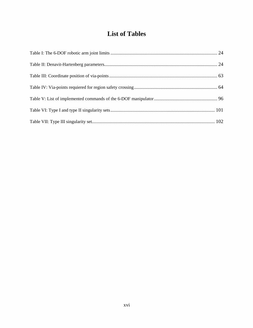
List of Tables
Table I: The 6-DOF robotic arm joint limits ...................................................................................... 24
Table II: Denavit-Hartenberg parameters ........................................................................................... 24
Table III: Coordinate position of via-points ....................................................................................... 63
Table IV: Via-points requiered for region safety crossing ................................................................... 64
Table V: List of implemented commands of the 6-DOF manipulator ................................................... 96
Table VI: Type I and type II singularity sets .................................................................................... 101
Table VII: Type III singularity set................................................................................................... 102
xvi

List of Symbols
𝑻𝒊𝒊−𝟏 Transformation matrix of the frame ( i ) with respect to frame ( i–1 )
𝒓𝒊𝒋 Element of the rotational matrix
𝒑𝒙 X Cartesian coordinates of the position vector
𝒑𝒚 Y Cartesian coordinates of the position vector
𝒑𝒛 Z Cartesian coordinates of the position vector
𝜽𝒊 ith joint angle of the manipulator
𝒅𝜽𝒊 Differential ith joint angle of the manipulator
𝑮𝜽 Global position vector
𝑱𝜽 Jacobian matrix
𝑫 Differential position vector
𝑫𝜽 Differential joint configuration vector
𝒅𝒑𝒙 Differential X Cartesian coordinates of the position vector
𝒅𝒑𝒚 Differential Y Cartesian coordinates of the position vector
𝒅𝒑𝒛 Differential Z Cartesian coordinate of the position vector
𝒙𝒊 X axis of the ith moving frame
𝒚𝒊 Y axis of the ith moving frame
xvii

𝒛𝒊 Z axis of the ith moving frame
𝒍𝒊 Length of the ith link of the manipulator
𝒔𝒊 Sine of the ith joint angle of the manipulator
𝒄𝒊 Cosine of the ith joint angle of the manipulator
𝒔𝒊𝒋 Sine of the sum of the ith and the jth joint angles of the manipulator
𝒄𝒊𝒋 Cosine of the sum of the ith and the jth joint angles of the manipulator
𝝅 Constant pi
𝑬 Link error paramenter
𝒂𝒕𝒂𝒏𝟐 Two-argument function used to compute the arctangent of 𝑥/𝑦, considering not only
the values, but the signs of the arguments.
𝒔𝒊 ith singularity set of the manipulator
𝒇(𝒊) Function of the ith singular parametric surface function
𝝋 Orientation of the manipulator end-effector
𝜶,𝜷,𝜸 Angle components of Euler orientation
𝒙𝒄,𝒚𝒄, 𝒛𝒄 Cartesian coordinates of the center of an ellipsoid
𝒙𝒓,𝒚𝒓, 𝒛𝒓 Radius components of an ellipsoid
xviii

Chapter 1
Introduction
1.1 Background
Nowadays, one of the most important concerns of society is the elderly and disabled care
assistance. Health care resources are becoming insufficient due to a progressively aging
population and rising of life expectancy. Strong efforts have been made to incorporate
technology to fulfill these needs. Carrying or moving objects from one place to another are some
of the challenging tasks faced by elderly, who may also suffer from pain or partial absence of
movement in their limbs. Simple tasks such as carrying medicine, food or water that require
walking from one room to another, grabbing the item, and continue walking may be difficult or
sometimes even impossible to accomplish. Nursing, is commonly used to assist patients on these
matters; however, it tends to be insufficient and/or costly service. Nowadays, robotics appears as
a suitable technology that can be implemented to perform some of these tasks.
To move an object from one place to another using a mobile robot, navigation and motion
control of the robot are required. This research, as part of a major project, is focused on the
motion control of a six degree-of-freedom (6-DOF) robot manipulator attached to a wheeled
mobile robot. A proper explanation on how the manipulator was chosen is presented. This
document contains simulation and experimental results of a project aimed to design and
implement an algorithm for motion of a robotic manipulator to accomplish pick-and-place
operations. Such operations must be performed avoiding stationary obstacles found in an indoor
room environment. The different approaches implemented to achieve the aforementioned tasks in
a 6-DOF manipulator are described in this thesis.
1

1.2 Objective
The general objective of this research project is to develop an algorithm to make a robotic
arm capable of accomplishing pick-and-place operations. Such operations involve moving an
object from an initial to a final given position while avoiding stationary obstacles. After
reviewing the literature of previous research done about manipulators motion, specific objectives
were established.
The specific objectives include:
1. To accurately describe the robotic arm configuration in order to compute the forward
kinematics equations.
2. To effectively solve the inverse kinematics problem with minimum computational effort.
3. To define the entire workspace of the manipulator (interior and exterior boundaries) in
order to design paths with reachable configurations.
4. To select an adequate end-effector orientation for any specific coordinate position so that
possible configurations of the manipulator are found.
5. To design a collision-free path to avoid stationary obstacles.
6. To evaluate the effectiveness of the proposed method by comparing simulation and
experimental results.
1.3 Problem Statement and Methodology
Small wheeled mobile robots represent a feasible solution for patient assistance in
medical care environments due to their compact design and simple operation. Basic tasks such as
carrying an object from one place to another require a manipulator to be attached to the wheeled
mobile robot, capable of reaching objects at any position and orientation inside its workspace. A
manipulator with a minimum of six joints (6-DOF) is needed to have six degrees of freedom
2

movement in the Cartesian coordinate system (three degrees of freedom for translation and three
for rotation). The robotic arm chosen in this research, which fulfills the aforementioned
requirement, is a 6-DOF manipulator composed by several individual modules and a gripper end-
effector. Both, the wheeled mobile robot and its manipulator, are shown in Figure 1.
(a)
(b)
Figure 1: 6-DOF manipulator: a) Wheeled mobile robot; b) Rotation angles
The algorithm proposed in the present document makes the robotic arm capable of
performing pick-and-place operations to manipulate objects as desired. Designing pick-and-place
operations requires the implementation of several robotic techniques: forward kinematics,
inverse kinematics, workspace and dexterity analysis, and collision-free path planning. The
forward kinematics equations are computed using an adequate description of the manipulator.
Such description is performed using the Denavit-Hartenberg (DH) notation [1]. An inverse
kinematic method capable of finding all possible solutions for the forward kinematics equations
is proposed. Such method combines the geometry and kinematics of the manipulator to derive
two non-linear simultaneous equations that can be solved with traditional numerical techniques.
Several configurations for the robot manipulator can be obtained at any position along a path.
3

Even when none of the multiple solutions can avoid the end-effector hitting an obstacle,
situations exist in which choosing the right solution avoids the body of the manipulator hitting
with such obstacle. As shown in Chapter 4, the inverse kinematic method proposed requires low
computational efforts to converge into multiple solutions, and can be applied in real time path
planning due to its acceptable performance. Predefined paths, as shown in Figure 2, were used to
test the effectiveness of the inverse kinematic method. The plot of the angular displacements of
the manipulator joints, presented in Figure 3, shows the required smooth transitions on the joint
motion of the manipulator. The complete analysis of results is presented in Chapter 4.
Figure 2: Predefined path used to evaluate the inverse kinematics methods
Figure 3: Angular joint displacement of the predefined path
4

To properly plan a path that remains within the manipulator operational area, an analysis
of the workspace of the manipulator is required. The workspace obtained for the 6-DOF
manipulator is shown in Figure 4. Every position point that lies inside the spherical workspace of
the manipulator shown in blue lines has at least one kinematic solution. The mobile robot
platform is represented by a yellow geometric shape.
Figure 4: Workspace of the manipulator
To find proper configurations of the manipulator along the path, the proposed algorithm
requires that the end-effector position remains within the workspace and has suitable
orientations. Throughout the analysis, each selected point, is analyzed to ensure that it falls
within the workspace boundaries. Even if a point is located inside the workspace of the
manipulator, a solution may only exist for specific orientations. A suitable range of Euler angles
orientation for the selected point is then derived using an analytical dexterity method.
5

To design a collision-free path, a route from the initial to the final given position is
traced. Via-points may be chosen with the path planning algorithm depending on the complexity
of the route required. Via-points are intermediate points through which the end-effector is forced
to pass. The path between via-points is then designed by tracing a straight line through a set of
points. To avoid obstacles, their volumes must virtually be enclosed by ellipsoids. If any point on
the straight line lies inside the ellipsoid boundary of an obstacle, it will be repelled to the
boundary limits. Finally, to avoid the manipulator joints hitting an obstacle, each joint movement
is analyzed. Simulation and experimental results confirm that the proposed method is capable of
performing the aforementioned operations by designing suitable paths. A typical planned path
which avoids four obstacles is shown in Figure 5. The via-points were strategically chosen to
avoid crossing the back of the manipulator or the center of the workspace regions in which the
manipulator can present motion difficulties.
Figure 5: Simulation of a free-collision path
6

Thesis outline
The thesis consists of five chapters, a references section and appendices. The content of
each chapter is briefly described as follows. Chapter 1 presents a brief introduction, objectives
and methodology of the project, and summary of results. Chapter 2 is a literature review of
previous research on inverse kinematics methods, workspace and dexterity analysis, and
manipulators path planning. Chapter 3 is the problem and analysis description. It presents an
accurate description of the manipulator used in this project formulated using a traditional
method. A new Iterative Inverse Kinematics (IIK) method, the analytical formulations to solve
the workspace and the dexterity of the robotic arm configuration, and a technique for planning an
obstacle-free path are also presented. In Chapter 4, simulation and experimental results are
described. By plotting the required computational effort, the performance of the proposed IIK
method is compared to the Newton’s method performance when using pseudo-inverse matrix.
The graphs of the static and dynamic manipulator joint variables, which are obtained from
several paths using the proposed collision-free design algorithm, are included. In Chapter 5,
conclusions and future work recommendations are presented.
7

Chapter 2
Literature Review
2.1 Introduction
To effectively accomplish pick-and-place operations, robotic arm description, inverse
kinematics solution, workspace and dexterity analysis, and collision-free path planning tasks are
required. A summary of relevant research methods involving the aforementioned tasks are
reviewed in this chapter. Some of the methods reviewed were implemented and adjusted for the
six degree of freedom (DOF) robotic arm used in this project.
2.2 Forward Kinematics Description
Forward kinematics refers to the geometrical representation of a coordinate frame located
at any part of the manipulator with respect to a fixed coordinate frame usually attached to the
base of the manipulator [2]. The most common analysis is made over the tip of the manipulator,
typically known as end-effector, where the tool of the manipulator is located. The formulation
derived from the forward kinematics is used to define the end-effector position and orientation.
Such formulation is a function of the manipulator joint angles. Denavit-Hartenberg (DH)
notation [2] is used in this project to describe the manipulator configuration. With this notation,
each link location is described by two angles and two distance parameters. When all the joints
and lengths of the manipulator are described, the entire robot manipulator structure can be
defined. Several interpretations about this notation have been made by different authors. Craig’s
representations [2], in which coordinate frames are located at the origin of each link, are used in
this research. Once the frames are defined, the offset parameters can be obtained and the
8

transformation matrices can be computed. Each transformation matrix relates a specific link of
the manipulator with respect to the link attached immediately to it. A homogenous
transformation, that contains information of the end-effector position and orientation, is
computed by multiplying all link transformations. The computation of the homogenous
transformation corresponding to a 6-DOF manipulator as shown in Figure 8 in Section 3.2 is
given below:
𝑇10 𝑇21 𝑇32 𝑇43 𝑇54 𝑇65 = �
𝑟11 𝑟12 𝑟13 𝑝𝑥𝑟21 𝑟22 𝑟23 𝑝𝑦𝑟31 𝑟32 𝑟33 𝑝𝑧0 0 0 1
� (1)
where, 𝑇𝑖𝑖−1 is the transformation matrix of the frame coordinate system of link ( 𝑖) with
respect to the frame coordinate system of the link (𝑖 − 1), where
𝑖 = 0,1,2…𝑛,
𝑟𝑖𝑗 is an element of the end-effector orientation matrix in the homogenous
transformation located in the ( 𝑖) row and the ( 𝑗) column, where
𝑖, 𝑗 = 1, 2,3 and,
𝑝𝑥,𝑝𝑦, and 𝑝𝑧 are the coordinate positions of the end-effector.
Finally trigonometric algebraic expressions are obtained by equating each matrix element
from both sides of Equation 1. Twelve non-linear equations, in which only six of them are
independent, are used to compute six unknowns when using a 6-DOF robotic arm. Such
equations are used to solve the inverse kinematics problem.
9

2.3 Inverse Kinematics Methods
In robotics, finding the joint angles of a manipulator to locate the end-effector at a given
position and orientation is known as inverse kinematics [2]. Solving the inverse kinematics
problem is essential for pick-and-place operations. Although the process may be complicated, the
most effective way to find the joint configurations is looking for the closed-form expression of
the manipulator. For some manipulators, such closed-form expression might not exist and a
numerical method has to be implemented to obtain an inverse kinematic solution. An iterative
procedure with progressive approximation often requires high computational effort and it only
yields to a unique solution. Also, such solution depends on the previous configuration of the
manipulator. A review of some of the analytical and numerical methods that were used in an
attempt to solve the joint angle configurations of the manipulator is briefly presented in the
following subsections.
2.3.1 Analytical Methods
An analytical method to solve the inverse kinematics was proposed by Craig [2], in
which twelve non-linear equations are derived using the DH notation. Since nine of those twelve
equations are computed from the 3x3 orthogonal matrix of rotation, these are dependent
equations. Only three non-linear independent equations and six unknowns can be derived from
the orthogonal matrix. Another three independent equations are derived by equating the
coordinate positions from both sides of Equation 1. Finally a system of six non-linear equations
with six unknowns is obtained. After analyzing the system of equations the closed-form
expression can be derived. Substitutions and trigonometric identities are usually needed to
simultaneously solve for the joint angles. Several attempts were made to try to find a closed-form
10

expression by implementing this method in the present research; however, none of those derived
into a feasible solution.
Vasilyev and Lyashin [3] developed a method to solve the inverse kinematics for 6-DOF
manipulators. Similar to Craig’s method [2], this approach derives the twelve overdetermined
non-linear equations from the DH notation. This method suggests three alternatives to generate
the three independent equations from the orthogonal matrix of rotation. The first method consists
of the parameterization of the rotation matrices from both sides of Equation 1 using Euler angles.
The three Euler angles expressions obtained from both sides are equalized to derive into three
independent equations. The second approach involves the application of Cayley transformation
into the 3x3 rotation matrices from both sides of Equation 1. Again, three independent equations
are derived; however, by using this transformation the matrices may take an indeterminate form.
These facts lead the authors to propose a third method. In this last method an adjustment of
Cayley transformation is used. As before, three independent equations are obtained. After getting
three independent equations using any of the aforementioned approaches, another three
independent equations are derived by equating the coordinate positions from both sides of
Equation 1. Sine and cosine functions are then replaced by tangents of half angles to transform
the trigonometric functions in algebraic functions. After implementing this method in the 6-DOF
manipulator used in this research, the formulations did not converge into a suitable solution.
A recent research performed by Shimizu et al [4], computes the analytic inverse
kinematics of a 7-DOF redundant manipulator. Such manipulator consists of several links
interconnected by seven revolute joints. The inverse kinematics problem is solved using an arm
angle parameter to represent the redundancy of the manipulator. The fourth joint is then derived
into a closed-form expression taking advantage of the spherical as shoulder base configuration.
11
Once the fourth joint is found, the other joints are simply computed using the inverse kinematics
equations. The manipulator used in [4], has a similar configuration to the one used in the present
research. The fourth joint derivation in the current project was not possible since the joint axes
from the first three joints do not intersect at a single point.
After reviewing and implementing the analytical methods explained above, the closed-
form expression for the 6-DOF manipulator used in this thesis was not found. This fact can be a
consequence of a nonexistence closed-form expression and suggests that an iterative inverse
kinematic approach is necessary.
2.3.2 Iterative Methods
Numerical Techniques such as Newton’s method can be used to obtain the joints
configuration; however, this method will converge to a single solution even though several
solutions may exist. Because of the overdetermined non-linear equations that describe the
manipulator used in this research, the Newton’s method requires the calculation of a pseudo-
inverse Jacobian matrix, which tends to be unstable near singularities [5]. Wampler overcame
this problem by implementing the damped least square method (DLS) which adds damping
coefficients into the inverse kinematics calculations. The damping coefficient is larger near the
singularities and unreachable solutions. However, this method is likely to oscillate if damping
coefficient is not chosen carefully [6]. Selectively damped least squares method (SDLS)
proposed by Buss and Kim [6], reduces oscillations by choosing the damping coefficient based
on the manipulator configuration and the distance to the target position.
An iterative approach for solving the inverse kinematics of a robotic arm was developed
by Grudić and Lawrence [7]. The Offset Modification method (OM) is used to find a model
12

manipulator configuration capable of deriving into closed-form inverse kinematics equations by
modifying the real manipulator offset parameters. Once the closed-form expressions are found,
multiple solutions for the joint angles of the model manipulator can be obtained. When the model
and the real manipulators have the same angle values, the pose of both end-effectors has the
same orientation but different position. Since this is true for any point to evaluate, three non-
linear equations with three unknowns can be derived from the difference in position of both
models. Such equations can be solved with standard numerical techniques. Whenever a solution
for the model manipulator is found, the numerical method used to solve the system of non-linear
equations will converge to a solution for the joints of the real manipulator. This ensures
convergence into multiple solutions when they exist. This method allows choosing one solution
among several, giving the robot arm the possibility of avoiding obstacles. The results shown in
[7] prove the effectiveness of the method, converging to the desired solution with relatively
small computational efforts. By setting the second link offset to zero, the configuration of the
manipulator used in the current research can be modified into a Pieper’s configuration [8], in
which three adjacent joint axes intersect in one point. Since Pieper’s configuration can generate
closed-form inverse kinematics equations, the OM method can be implemented for the present
project. The main disadvantage of this method compared with that used in this research is the
computational time required to solve the inverse kinematics. Several iterations to find the
multiple solutions are needed when using the OM method.
Another approach for solving the inverse kinematics of a 6-DOF manipulator is presented
by Siciliano [9]. In this method a closed-loop dynamic system is used to solve the inverse
kinematics problem of a 6-DOF manipulator. As with any inverse kinematics problem, the input
of the system is the desired position and orientation of the end-effector. Since the
13

aforementioned system is a second order system, the outputs generated are the angular position,
velocity and acceleration needed to control the manipulator joints in a torque-like control
scheme. The method proposed by Siciliano is based on the computation of the Jacobian
transpose to keep tracking of the desired path. This technique avoids the problems related to
matrix inversion usually presented with numerical methods. Since the computation of the
Jacobian transpose is fast, the computational efforts are minimum as compared to the matrix
inversion methods. It is been clearly demonstrated by Siciliano that the performance of this
method is effective; however, it requires high control skills.
The Iterative Inverse Kinematics method (IIK) based on the geometry of the 6-DOF
manipulator is proposed in this thesis to solve the inverse kinematics problem. This method is
capable of finding multiple solutions, if they exist, at any given position and orientation. In order
to solve the first two joint angles of the manipulator configuration, the kinematics expressions
are derived into two non-linear trigonometric equations. The roots that satisfy both equations are
computed using the bisectional method. The rest of the joint angles are easily derived by
substituting the roots found into the kinematics expressions. Some of the concepts used to
develop this approach were obtained from the aforementioned methods. The complete analysis
and formulations are presented in Section 3.3.
2.4 Workspace Analysis
The workspace of a manipulator comprises all reachable points of the robot end-effector.
During path planning, knowing the workspace of a manipulator is essential since it determines
the manipulator operating limits. The workspace of a robotic arm is fully related to its
singularities. Therefore, the knowledge of singular configurations is of great importance. These
14
configurations also dictate the manipulator movement capabilities. Abdel-Malek [10] developed
an analytical method to determine the interior and exterior boundaries of serial chain
manipulators by identifying singular surfaces [11, 12]. Such singular surfaces are generated
using the singular configurations of the manipulator. Most of the singularities occur when two or
more links are lined up, or when two or more joints have reached their limits. Singularities are
calculated by looking for the row-rank deficiency conditions of the Jacobian matrix. According
to Abdel-Malek and Yeh [12] there are three types of singularities: rank-deficiency singularity
set, rank-deficiency of the reduced-order accessible set, and constraint singularity set. Several
singular surfaces can be derived using this method; however, not all of these are part of the
manipulator boundaries. Abdel-Malek [10] proposed a method to define which singular surfaces
belong to the workspace boundary. This method computes possible directions of motion of a
point located on the evaluated surface by calculating the sign of its normal acceleration.
Implementation of this method for the 6-DOF manipulator is described in Chapter 3.
2.4.1 Jacobian of the Manipulator
In robotics, the Jacobian is the derivative of the end-effector position of a manipulator
with respect to time [13]. In this project, the Jacobian relates the linear velocities of the end-
effector to the angular velocity of the joints. The Jacobian is obtained by taking the partial
derivatives of the end-effector position in the global Cartesian coordinate with respect to each
joint variable. The Jacobian matrix is a function of time since each joint changes with respect to
time. The Jacobian matrix is essential in the generation of robotic arm trajectories. According to
Abdel-Malek and Yeh [11], when a serial manipulator is at singular configurations, its Jacobian
matrix also becomes singular. The method to determine singular configurations of a matrix
depends on whether it is squared or not. The set of variables that makes a square matrix singular
15
is obtained by equating its determinant to zero. Alternatively, when the matrix is not square, the
set of variables is obtained by making the matrix rank-deficient. The Jacobian matrix computed
for most of the serial manipulators, as the one used in this project, is not squared.
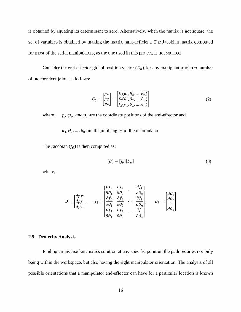
Consider the end-effector global position vector (𝐺𝜃) for any manipulator with 𝑛 number
of independent joints as follows:
𝐺𝜃 = �
𝑝𝑥𝑝𝑦𝑝𝑧� = �
𝑓1(𝜃𝜃1,𝜃𝜃2, … ,𝜃𝜃𝑛)𝑓2(𝜃𝜃1,𝜃𝜃2, … ,𝜃𝜃𝑛)𝑓3(𝜃𝜃1,𝜃𝜃2, … ,𝜃𝜃𝑛)
� (2)
where, 𝑝𝑥,𝑝𝑦, and 𝑝𝑧 are the coordinate positions of the end-effector and,
𝜃𝜃1, 𝜃𝜃2, … , 𝜃𝜃𝑛 are the joint angles of the manipulator
The Jacobian (𝐽𝜃) is then computed as:
[𝐷] = [𝐽𝜃][𝐷𝜃] (3)
where,
𝐷 = �𝑑𝑝𝑥𝑑𝑝𝑦𝑑𝑝𝑧
� , 𝐽𝜃 =
⎣⎢⎢⎢⎢⎢⎡𝜕𝑓1𝜕𝜃𝜃1
𝜕𝑓1𝜕𝜃𝜃2
⋯𝜕𝑓1𝜕𝜃𝜃𝑛
𝜕𝑓2𝜕𝜃𝜃1
𝜕𝑓2𝜕𝜃𝜃2
⋯𝜕𝑓2𝜕𝜃𝜃𝑛
𝜕𝑓3𝜕𝜃𝜃1
𝜕𝑓3𝜕𝜃𝜃2
⋯𝜕𝑓3𝜕𝜃𝜃𝑛⎦
⎥⎥⎥⎥⎥⎤
, 𝐷𝜃 = �
𝑑𝜃𝜃1𝑑𝜃𝜃2⋮
𝑑𝜃𝜃𝑛
�
2.5 Dexterity Analysis
Finding an inverse kinematics solution at any specific point on the path requires not only
being within the workspace, but also having the right manipulator orientation. The analysis of all
possible orientations that a manipulator end-effector can have for a particular location is known
16

as local dexterity. An iterative method to find the local dexterity solutions for any serial chain
manipulators is presented by Abdel-Malek and Yeh [14].
According to [14], to determine admissible orientations of the end-effector at any specific
point, tracing a sphere around the point is needed. Such sphere is called the service sphere, which
must have a radius equal to the length of the manipulator last link. For any point reached by the
end-effector of the manipulator, possible orientations can be determined by evaluating all
reachable points by the second-last-joint (SLJ) of the manipulator without changing the target
position. The intersection of the SLJ space boundary (interior and exterior) with the service
sphere defines the service region, which is the region of feasible penetration orientations of the
manipulator last link into the service sphere. This region derives into possible orientations for the
manipulator end-effector. The service sphere and service region for the 6-DOF manipulator used
in this research are shown in Figure 6.
Figure 6: Service sphere and region for the 6-DOF manipulator
17

Since this method is intended to work for any serial chain manipulator, Abdel-Malek and
Yeh [14] proposed a continuation method to find the intersection of the SLJ with the service
sphere; however, an analytical formulation is derived for the 6-DOF robotic manipulator used in
this research and is presented in this document.
2.6 Collision-free path planning
In order to design a collision-free path for the 6-DOF manipulator, different methods are
combined, modified and implemented. A method to accomplish pick-and-place operations was
recently developed at the University of Saskatchewan by Fotouhi et al [15]. This method defines
two via-points between the initial and final given positions such that the end-effector avoids
stationary obstacles. Via-points are intermediate points through which the end-effector is forced
to pass. The path is then broken into three segments. To keep track of those segments, two
different approaches were used: Linear End-effector Increment (LEI) and Linear Joints
Increment (LJI). In LEI method, the segments between via-points are linearly divided into
several steps, and for each step, the joint angles are calculated by an inverse kinematic method.
Difficulties caused by such inverse kinematics method may increase as the division steps
increase. In the LJI method, joint angle positions are calculated only for initial, final and via-
points positions. The segments between via-points are therefore tracked by increasing the joint
angles linearly. Complications caused by the inverse kinematic process decrease as a
consequence. Although the LJI method does not follow the given path exactly, the results
presented in [15] show that the LJI method is efficient and requires low computational efforts. It
has been observed that if the division steps on the LEI method are reduced, its performance
becomes similar to the performance of the LJI method. For the project presented in this thesis, in
18
which the path must be accurately followed, the LEI method is implemented and the division
steps are set according to the end-effector displacement.
A technique used to avoid collisions between a redundant manipulator and obstacles is
proposed by Ping et al [16]. In this method, the manipulator path and obstacles are mapped into
the robot arm workspace. To keep the robot arm within the collision-free path, safety zones
around obstacles are defined. When any part of the robot arm enters an obstacle safety zone, a
virtual force pushes that part away without changing the end-effector position. This task can be
fully accomplished only for redundant manipulators. When the end-effector reaches an obstacle
safety zone, the original path must be re-planned. The virtual forces from the safety zone are
modeled as a spring-damper system, such that the repulsion force is proportional to the
penetration length. The simulations and experimental results given in [16] are an indication of
effectiveness of their method. Since the 6-DOF manipulator used in this research is not a
redundant manipulator, only part of this method can be implemented.
An obstacle avoidance approach for robotic manipulators is presented by Zhang and Sobh
[17]. In this method the initial and final positions and orientations of the end-effector are given,
and these represent the manipulator pose to pick or release an object. The algorithm generates
intermediate points between the actual position and the goal position of the manipulator, if
required. Then, the path is designed using a cubic polynomial profile to fit the actual position,
the goal position, and the intermediate points without stopping at every point. The path is also
constrained to given desired joint velocity and acceleration. All the obstacles are mapped into the
coordinate system as cubic volumes and these are completely enclosed by a sphere. In order to
avoid hitting an obstacle, intermediate points are defined such that these reside outside the
obstacle sphered boundary. The links should also stay outside the sphered boundary. The
19

algorithm presented in [17], therefore, keep track of the closest distance from the obstacle center
to any part of the manipulator links, and redesign the path if such distance is less than the radius
of the sphered boundary.
A manipulator path planning algorithm capable of planning collision-free trajectories is
proposed by Lin [18]. The algorithm is composed by two planners: a Global Path Planner (GPP)
and a Local Motion Planner (LMP). The GPP consists of mapping obstacles within the
workspace of the manipulator and defines convex regions of free space. Any path traced within
these regions has an obstacle-free straight line path. To ensure a secure path from one region to
another, the algorithm establishes safety cross points at each side of free-space region that is
adjoined to another free-space region. If more than one path is capable of reaching the final
position by crossing several free-space regions, the algorithm selects the shortest distance path.
Once the global path is generated, the algorithm adds more intermediate points to achieve a finer
trajectory. The LMP consists of selecting optimal configurations for the manipulator along the
path. Since a single point position can be reached by the manipulator with more than one
configuration, such configurations could change abruptly while following the path. LMP ensures
smooth joint transitions along the path using a mimetic algorithm. This algorithm uses a vector
of variables called chromosome containing the joint angular displacements or genes, which are
assigned to the manipulator configuration. Such chromosomes are capable of evolving and
learning to create new smooth trajectory profiles.
20
Chapter 3
Problem Description and Analysis
3.1. Introduction
The present chapter provides a detailed description of different analyses implemented for
the 6-DOF robot manipulator. Some of the methods described in Chapter 2 were modified and
adjusted based on the general characteristics of the 6-DOF robotic arm. Even though some
methods were not feasible to be fully implemented for the 6-DOF manipulator used in this
research, some practices used by the authors of these methods were applied. Additional analysis,
used to solve specific problems occurring throughout the solution process, is also presented.
Pick-and-place operations can be performed by separating such operations into several
tasks to be solved individually. The following tasks and their solutions are explained in this
chapter: 1) deriving forward kinematics equations based on the description of the manipulator, 2)
solving the inverse kinematics problem, 3) computing of the workspace the manipulator and its
representation in the Cartesian coordinate system, 4) determining the end-effector orientation, 5)
designing a global path to avoid areas within the workspace where the manipulator has motion
control difficulties and, 6) planning collision-free paths to avoid stationary obstacles based on a
repulsive potential field. The simulator used to verify the performance of the algorithm and the
program designed to interact with the user are also described in this chapter. Finally, all the
analyses and calculations generated by developing the aforementioned tasks are given in this
chapter.
21
3.2. Manipulator Description
The 6-DOF robotic arm used in this project is a serial chain manipulator composed of
several modules and a gripper end-effector interconnected by six revolute joints as presented in
Figure 7. The aforementioned modules can be squared or cylindrical units as shown in Figure 7a.
Each module has a built-in brushless servomotor capable of delivering torque of 372Nm on the
squared units and 239Nm on the cylindrical units. The maximum speed reached by the modules
is 8.2 rad/s for the squared units and 1.2 rad/s for the cylindrical units. Such modules also contain
incremental encoders for positioning and speed control and have fully integrated power and
control electronics. These modules are capable of rotating more than 360 degrees but have
spacing limitations due to the manipulator configuration.
The analysis is initiated by choosing the joint angle limits, as shown in Table I, to avoid
hitting the manipulator itself. All modules were commanded with a Controller Area Network
(CAN) communication system. Although several programming functions exist to control the
robot manipulator, only certain functions were implemented. A summary of the functions used
for this project is presented in Appendix A. As mentioned in Chapter 2, the Denavit-Hartenberg
(DH) notation was used in this research to describe the manipulator kinematics. The coordinate
frame locations following Craig’s convention [2] are shown in Figure 8. Each frame was located
at the origin axis of each link, and its z axis direction was chosen according to the positive
rotation of the real manipulator using the right-hand rule. The DH parameters that correspond to
the initial position configuration shown in Figure 8 are given in Table II.
22

(a)
(b)
Figure 7: Robotic arm configuration: a) The 6-DOF manipulator; b) Rotation angles
Figure 8: Global and moving coordinate frames of the manipulator in home position
23

Table I: The 6-DOF robotic arm joint limits
Joint Lower Limit Upper Limit
1 -160° 160°
2 -120° 95°
3 -160° 160°
4 -119° 119°
5 -119° 119°
6 -180° 180°
Table II: Denavit-Hartenberg parameters
Frame ( i ) 𝛼𝑖−1 𝑎𝑖−1 𝑑𝑖 𝜃𝜃𝑖 1 0 0 𝑙1 𝜃𝜃1 2 −90° 𝑙2 0 𝜃𝜃2 − 90° 3 −90° 0 𝑙3 𝜃𝜃3 4 −90° 0 0 𝜃𝜃4 − 90° 5 0 𝑙4 0 𝜃𝜃5 + 90° 6 −90° 0 −𝑙5 𝜃𝜃6
To keep the initial position configuration as the home position as shown in Figure 8, in
which all the joint angles are zero, the joint variables (𝜃𝜃𝑖) were adjusted +90° or −90° as shown
in Table II. Considering the aforementioned adjustment and based on Craig’s convention [2] the
homogenous transformation that relates the end-effector position and orientation with the global
coordinate system is given by:
24

𝑇60 = 𝑇10 𝑇21 𝑇32 𝑇43 𝑇54 𝑇65 = �
𝑟11 𝑟12 𝑟13 𝑝𝑥𝑟21 𝑟22 𝑟23 𝑝𝑦𝑟31 𝑟32 𝑟33 𝑝𝑧0 0 0 1
� (4)
where,
𝑟11 = 𝑐6[𝑐45(𝑠1𝑠3 + 𝑐1𝑠2𝑐3) − 𝑠45𝑐1𝑐2]− 𝑠6[𝑠1𝑐3 − 𝑐1𝑠2𝑠3]
𝑟21 = 𝑠6[𝑐1𝑐3 + 𝑠1𝑠2𝑠3] − 𝑐6[𝑐45(𝑐1𝑠3 − 𝑠1𝑠2𝑐3) + 𝑠45𝑠1𝑐2]
𝑟31 = 𝑐6(𝑠45𝑠2 + 𝑐45𝑐2𝑐3) + 𝑐2𝑠3𝑠6
𝑟12 = −𝑠6[𝑐45(𝑠1𝑠3 + 𝑐1𝑠2𝑐3) − 𝑠45𝑐1𝑐2]− 𝑐6[𝑐3𝑠1 − 𝑐1𝑠2𝑠3]
𝑟22 = 𝑠6[𝑐45(𝑐1𝑠3 − 𝑠1𝑠2𝑐3) + 𝑠45𝑠1𝑐2] + 𝑐6[𝑐1𝑐3 + 𝑠1𝑠2𝑠3]
𝑟32 = 𝑐2𝑠3𝑐6 − 𝑠6(𝑠45𝑠2 + 𝑐45𝑐2𝑐3)
𝑟13 = −𝑠45(𝑠1𝑠3 + 𝑐1𝑠2𝑐3) − 𝑐45𝑐1𝑐2
𝑟23 = 𝑠45(𝑐1𝑠3 − 𝑠1𝑠2𝑐3) − 𝑐45𝑠1𝑐2
𝑟33 = 𝑐45𝑠2 − 𝑠45𝑐2𝑐3
𝑝𝑥 = 𝑙2𝑐1 + 𝑙3𝑐1𝑐2 + (𝑙5𝑠45 + 𝑙4𝑠4)(𝑠1𝑠3 + 𝑐1𝑠2𝑐3) + (𝑙5𝑐45 + 𝑙4𝑐4)(𝑐1𝑐2)
𝑝𝑦 = 𝑙2𝑠1 + 𝑙3𝑠1𝑐2 − (𝑙5𝑠45 + 𝑙4𝑠4)(𝑐1𝑠3 − 𝑠1𝑠2𝑐3) + (𝑙5𝑐45 + 𝑙4𝑐4)(𝑠1𝑐2)
𝑝𝑧 = 𝑙5(𝑠45𝑐2𝑐3 − 𝑐45𝑠2) + 𝑙4(𝑐2𝑐3𝑠4 − 𝑐4𝑠2) − 𝑙3𝑠2 + 𝑙1
All the joint variables used in Equation 4 were measured with respect to the home
position as shown in Figure 8. The notation 𝑟𝑖𝑗 in Equation 4 represents the elements of rotation
matrix, and 𝑝𝑖𝑗 the elements of the position vector, 𝑐𝑖 stands for 𝑐𝑜𝑠 (𝜃𝜃𝑖), 𝑠𝑖 for 𝑠𝑖𝑛 (𝜃𝜃𝑖), 𝑐𝑖𝑗 for
𝑐𝑜𝑠 (𝜃𝜃𝑖 + 𝜃𝜃𝑗), and 𝑠𝑖𝑗 for 𝑠𝑖𝑛 (𝜃𝜃𝑖 + 𝜃𝜃𝑗). All link transformations are presented in Appendix B.
25

3.3. Iterative Inverse Kinematics
The Iterative Inverse Kinematics (IIK) method proposed in this research consisted of
deriving two simultaneous non-linear equations based on the geometrical configuration of the
manipulator. Such equations can be derived in terms of the first and second joint angles 𝜃𝜃1 and
𝜃𝜃2 of the manipulator. As for any inverse kinematics method, the position and orientation of the
end-effector are known. After finding the two simultaneous equations, the problem becomes that
of solving a system of two nonlinear equations. The roots of this system of equations represent
the solutions, which are calculated using a bisectional method. Once joint angles 𝜃𝜃1 and 𝜃𝜃2 are
calculated, joint angle 4 is computed using the Law of cosines. The remaining joint angles are
calculated using kinematics equations from Equation 4.
3.3.1. Calculating joint angles 𝜃𝜃1 and 𝜃𝜃2
In order to obtain two simultaneous equations, the geometrical configuration of the
manipulator is considered. The robot manipulator is modeled in the Cartesian coordinate system
to analyze its geometrical configuration as shown in Figure 9. Letters A, B, C, D and E are
assigned to each manipulator joint to identify its position. Since the rotation axes at joints C and
D are parallel to each other and, the segments 𝐵𝐶�����⃗ and 𝐸𝐷�����⃗ are both normal to these rotation axes,
it can be inferred that the points B, C, D and E are in one plane regardless of the joints angles
value as shown in Figure 9a.
The previous statement derived into the following expression:
�𝐸𝐷�����⃗ × 𝐷𝐶�����⃗ � ∙ 𝐵𝐶�����⃗ = 0 (5)
where, segment 𝐸𝐷�����⃗ corresponds to the end-effector z-axis orientation vector
[𝑟13 𝑟23 𝑟33]𝑇 from equation 4.
26

To compute Equation 5, 𝑥,𝑦 and 𝑧 variables were assigned to each coordinate point as
shown in Figure 9b. In order to simplify the analysis, the global coordinate system was displaced
along its positive z-axis a distance equal to 𝑙1.
(a)
(b)
Figure 9: Schematic diagram of the 6-DOF Manipulator: (a) Plane BCDE; (b) Vector form
From Figure 9b, positions of points 𝑝𝐵 and 𝑝𝐶 can be expressed as:
𝑝𝐵 = [(𝑙2c1) (𝑙2𝑠1) 0] (6)
𝑝𝐶 = [(𝑙2𝑐1 + 𝑙3𝑐2𝑐1) (𝑙2𝑠1 + 𝑙3𝑐2𝑠1) (−𝑙3𝑠2)] (7)
Substituting and simplifying Equations 6 and 7 into Equation 5, the following expression
for the first simultaneous equation is obtained:
27

(𝑟23𝑧𝐷 − 𝑟33𝑦𝐷)𝑐2𝑐1 + (𝑟33𝑥𝐷 − 𝑟13𝑧𝐷)𝑐2𝑠1 + (𝑟23𝑥𝐷 − 𝑟13𝑦𝐷)𝑠2 + 𝑟13𝑙2𝑠1𝑠2
− 𝑟23𝑙2𝑐1𝑠2 = 0 (8)
Solving for 𝜃𝜃2 in Equation 8 the following expression is obtained:
tan(𝜃𝜃2) =
(𝑟23𝑧𝐷 − 𝑟33𝑦𝐷)𝑐1 + (𝑟33𝑥𝐷 − 𝑟13𝑧𝐷)𝑠1±[(𝑟23𝑥𝐷 − 𝑟13𝑦𝐷) + 𝑟13𝑙2𝑠1 − 𝑟23𝑙2𝑐1]
(9)
where,
𝑥𝐷 = 𝑝𝑥 − 𝑟13𝑙5 (9a)
𝑦𝐷 = 𝑝𝑦 − 𝑟23𝑙5 (9b)
𝑧𝐷 = 𝑝𝑧 − 𝑙1 − 𝑟33𝑙5 (9c)
The ± sign found in the denominator of Equation 9, was obtained when considering two
possible solutions for the dot product in Equation 5. The dot product is always zero for both the
positive and the negative values of perpendicular angles (±90°).
The second simultaneous equation is found by computing the length of the segments
𝐵𝐶�����⃗ and 𝐷𝐶�����⃗ . The magnitudes of these segments are known as they are the offset links parameters
from table I. The following equation was obtained:
�𝐵𝐶�����⃗ � + �𝐷𝐶�����⃗ � − 𝑙3 − 𝑙4 = 0 (10)
Substituting and simplifying Equations 6 and 7 into the left-hand side of Equation 10, the
following error nonlinear equation ‖𝐸‖ is computed as:
‖𝐸‖ = 𝑥𝐷2 + 𝑦𝐷2 + 𝑧𝐷2 + 𝑙22 + 𝑙32 − 𝑙42 − 2(𝑙2 + 𝑙3𝑐2)(𝑥𝐷𝑐1 + 𝑦𝐷𝑠1) + 2𝑙3(𝑧𝐷𝑠2 + 𝑙2𝑐2) (11)
28

The solution is found when both Equations 9 and 10 are satisfied, making Equation 11
equals to zero. To satisfy Equations 9 and 10 simultaneously using a bisectional method, a set of
values for joint angle 𝜃𝜃1 was substituted into equation 9 to obtain a set of values for joint angle
𝜃𝜃2. These two sets were substituted in Equation 11. The set of values of 𝜃𝜃1 and 𝜃𝜃2 which make
Equation 11 equal zero, represent the solution for joint angles 𝜃𝜃1 and 𝜃𝜃2 as shown in Figure 10.
Since the random values chosen as an initial guess for joint 𝜃𝜃1 set were likely not equal to zero in
Equation 11, a change of sign was evaluated. The change of sign over a particular interval
represents a zero crossing, and suggested the existence of a solution. An iteration process was
done at these intervals to obtain an accurate result.
Figure 10: Finding the roots for equation 11
To avoid misdetection when finding the roots of long intervals (Equation 11 could be
equal to zero twice inside an interval keeping the same sign at both ends), maximum and
minimum length error ‖𝐸‖ (i.e. Equation 11) were calculated and included into the joint angle 𝜃𝜃1
set. It was found that the minimum error occurred when joint angle 𝜃𝜃1 was oriented toward the
end-effector. The maximum error occurred when joint angle 𝜃𝜃1 was oriented to the opposite side.
29

𝑚𝑖𝑛 = 𝑎𝑡𝑎𝑛2(𝑝𝑦,𝑝𝑥) (12) 𝑚𝑎𝑥 = 𝑎𝑡𝑎𝑛2�𝑝𝑦,𝑝𝑥� ± 𝜋 (13)
The atan2 function computes the angle formed between the x and y components given
considering not just its values but also its signs.
3.3.2. Calculating joint angle 𝜃𝜃4
Using the Law of Cosines on the triangle formed by A, B and C in figure 9a, θ4 was
calculated as:
𝑐4 =
𝑥𝐷2 + 𝑦𝐷2 + 𝑧𝐷2 + 𝑙22 − 𝑙32 − 𝑙42 − 2𝑙2(𝑥𝐷𝑐1 − 𝑦𝐷𝑠1)2𝑙3𝑙4
(14)
𝑠4 = ±�1 − 𝑐42 (15)
𝜃𝜃4 = 𝑎𝑡𝑎𝑛2(𝑠4, 𝑐4) (16)
Two different configurations were obtained per each 𝜃𝜃1 solution as shown in Equation
15. This behavior, as stated by Gudric [7], allowed direct control over several configurations. In
this particular case, elbow-up or elbow-down could be chosen.
3.3.3. Calculating joint angle 𝜃𝜃3
Considering that the position vector of the fifth joint, 𝑥𝐷 ,𝑦𝐷 and 𝑧𝐷 parameters, are
known from Equation 9b, the following transformation is implemented:
𝑇50 = 𝑇20 𝑇52 (17)
30

Rewriting Equation 17 and pre-multiplying by [ 𝑇(𝜃𝜃1,𝜃𝜃2)20 ]−1, the dependence of the
joint angles 𝜃𝜃1 and 𝜃𝜃2 was transferred to the left hand side, obtaining the following equation:
𝑇20 −1 T50 = 𝑇52
where,
𝑇20 −1 = �
𝑐1𝑠2 𝑠1𝑠2 𝑐2 −𝑙1𝑐2 − 𝑙2𝑠2𝑐1𝑐2 𝑠1𝑐2 −𝑠2 𝑙1𝑠2 − 𝑙2𝑐2−𝑠1 𝑐1 0 0
0 0 0 1
�
T50 = �
× × × 𝑥𝐷× × × 𝑦𝐷× × × 𝑧𝐷0 0 0 1
�
𝑇52 = �
𝑐3𝑐45 −𝑐3𝑠45 −𝑠3 𝑙4𝑐3𝑠4−𝑠45 −𝑐45 0 𝑙4𝑐4 + 𝑙3−𝑠3𝑐45 𝑠3𝑠45 −𝑐3 −𝑙4𝑠3𝑠4
0 0 0 1
�
(18)
where × can be any value because they are not considered in these calculations.
Equating the (3, 4) elements from both sides:
( 𝑇20 −1 T50 )34 = 𝑐1𝑦𝐷 − 𝑠1𝑥𝐷 = −𝑙4𝑠3𝑠4 = 𝑇52 34 (19)
Then, 𝜃𝜃3 is obtained as:
𝑠3 =𝑠1𝑥𝐷 − 𝑐1𝑦𝐷
𝑙4𝑠4 (20)
𝑐3 = ±�1 − 𝑠32 (21)
𝜃𝜃3 = 𝑎𝑡𝑎𝑛2(𝑠3, 𝑐3) (22)
31

As before, two different configurations are obtained for 𝜃𝜃3. Combining 𝜃𝜃3 and 𝜃𝜃4
solutions, four different configurations per 𝜃𝜃1 solution are found.
3.3.4. Calculating joint angle 𝜃𝜃5
From Equation 4, the following expression is obtained:
𝑇60 = 𝑇20 𝑇62 (23)
Rewriting Equation 23 and transferring 𝜃𝜃1 and 𝜃𝜃2 to the left hand side we have:
[ 𝑇20 (𝜃𝜃1,𝜃𝜃2)]−1 T60 = 𝑇62
where,
𝑇20 −1 = �
𝑐1𝑠2 𝑠1𝑠2 𝑐2 −𝑙1𝑐2 − 𝑙2𝑠2𝑐1𝑐2 𝑠1𝑐2 −𝑠2 𝑙1𝑠2 − 𝑙2𝑐2−𝑠1 𝑐1 0 0
0 0 0 1
�
T60 = �
𝑟11 𝑟12 𝑟13 𝑝𝑥𝑟21 𝑟22 𝑟23 𝑝𝑦𝑟31 𝑟32 𝑟33 𝑝𝑧0 0 0 1
�
𝑇62 = �
× × −𝑐3𝑠45 ×× × −𝑐45 ×× × × ×0 0 0 1
�
(24)
Equating the (1, 3) and (2, 3) elements for both sides, the following expressions were
obtained:
𝑟13𝑐1𝑠2 + 𝑟23𝑠1𝑠2 + 𝑟33𝑐2 = −𝑐3𝑠45 (25)
𝑟13𝑐1𝑐2 + 𝑟23𝑠1𝑐2 − 𝑟33𝑠2 = −𝑐45 (26)
32
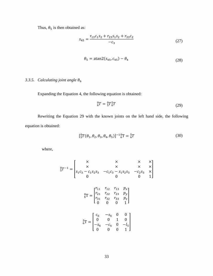
Thus, 𝜃𝜃5 is then obtained as:
𝑠45 =𝑟13𝑐1𝑠2 + 𝑟23𝑠1𝑠2 + 𝑟33𝑐2
−𝑐3 (27)
𝜃𝜃5 = atan2(𝑠45, 𝑐45) − 𝜃𝜃4 (28)
3.3.5. Calculating joint angle 𝜃𝜃6
Expanding the Equation 4, the following equation is obtained:
𝑇60 = 𝑇50 𝑇65 (29)
Rewriting the Equation 29 with the known joints on the left hand side, the following
equation is obtained:
[ 𝑇50 (𝜃𝜃1,𝜃𝜃2,𝜃𝜃3, 𝜃𝜃4,𝜃𝜃5)]−1 T60 = 𝑇65
where,
𝑇50 −1 = �
× × × ×× × × ×
𝑠1𝑐3 − 𝑐1𝑠2𝑠3 −𝑐1𝑐3 − 𝑠1𝑠2𝑠3 −𝑐2𝑠3 ×0 0 0 1
�
T60 = �
𝑟11 𝑟12 𝑟13 𝑝𝑥𝑟21 𝑟22 𝑟23 𝑝𝑦𝑟31 𝑟32 𝑟33 𝑝𝑧0 0 0 1
�
T65 = �
𝑐6 −𝑠6 0 00 0 1 0−𝑠6 −𝑐6 0 −𝑙5
0 0 0 1
�
(30)
33

Equating the (3, 1) and (3, 2) elements for both sides, the following expressions were
obtained:
𝑟11(𝑠1𝑐3 − 𝑐1𝑠2𝑠3) − 𝑟21(𝑐1𝑐3 + 𝑠1𝑠2𝑠3) − 𝑟31(𝑐2𝑠3) = −𝑠6 (31)
𝑟12(𝑠1𝑐3 − 𝑐1𝑠2𝑠3) − 𝑟22(𝑐1𝑐3 + 𝑠1𝑠2𝑠3) − 𝑟32(𝑐2𝑠3) = −𝑐6 (32)
Finally, 𝜃𝜃6 is computed as:
𝜃𝜃6 = atan2(𝑠6, 𝑐6) (33)
Once all the joint angles were computed, these were verified by substituting such angles
into the homogenous transformation from Equation 4. Since to calculate the manipulator joint
angles, the position and orientation of the end-effector were used, the homogenous
transformation obtained after the substitution had the same orientation and position as the input
values used. As discussed before, up to four possible configurations can be obtained for each
joint 𝜃𝜃1 solution. Since at least two sets of 𝜃𝜃1 and 𝜃𝜃2 values satisfy equations 9 and 11, the IIK
method can converge up to 8 different solutions. Special cases have been observed in which 16
solutions can be obtained. The multiple solutions obtained with the IIK method represent an
advantage over the single solution obtained with the Newton’s method when obstacle avoidance
is required. The criterion to choose one solution among the others along a desired path is based
on the closest configuration to that chosen in the previous position, provided that the manipulator
does not hit the obstacle. This criterion and its formulation are explained in detail in Section 4.2.
34

3.4. Workspace of the manipulator
As previously discussed in Section 2.4 the workspace of a manipulator comprises all
reachable point of the robot end-effector. During path planning, knowing the workspace of a
manipulator is essential since it determines the manipulator operation limits. If a specific
position, which is outside the workspace boundary, is given in the inverse kinematics analysis,
an error in the joint angle calculations may occur. According to the Abdel-Malek method [10],
two steps were followed in order to determine the workspace boundaries of the manipulator. The
first step consisted of finding all the manipulator singular parametric surfaces. At this step the
computation of the Jacobian was needed. The second step was to determine whether the singular
surfaces are boundaries or not. This second was achieved by identifying the permissible direction
of motion when crossing the singular surfaces [10].
3.4.1. Computing the Jacobian matrix
Considering the end-effector global position vector (𝐺𝜃) for the 6-DOF manipulator
extracted from Equation 4, the joint angle 𝜃𝜃6 does not affect such position:
𝐺𝜃 = �
𝑝𝑥𝑝𝑦𝑝𝑧� = �
𝑓1(𝜃𝜃1,𝜃𝜃2, 𝜃𝜃3, 𝜃𝜃4,𝜃𝜃5)𝑓2(𝜃𝜃1, 𝜃𝜃2, 𝜃𝜃3,𝜃𝜃4,𝜃𝜃5)𝑓3(𝜃𝜃2,𝜃𝜃3,𝜃𝜃4,𝜃𝜃5)
� (34)
where 𝑓1, 𝑓2 and 𝑓3 are the Cartesian coordinate position function of joint angles 𝜃𝜃1, 𝜃𝜃2, 𝜃𝜃3, 𝜃𝜃4
and 𝜃𝜃5 as shown in the following expressions:
𝑓1(𝜃𝜃1,𝜃𝜃2,𝜃𝜃3,𝜃𝜃4,𝜃𝜃5) = 𝑙2𝑐1 + 𝑙3𝑐1𝑐2 + (𝑙5𝑠45 + 𝑙4𝑠4)(𝑠1𝑠3 + 𝑐1𝑠2𝑐3) + (𝑙5𝑐45 + 𝑙4𝑐4)(𝑐1𝑐2) (34a)
35
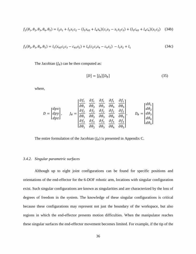
𝑓2(𝜃𝜃1,𝜃𝜃2,𝜃𝜃3,𝜃𝜃4, 𝜃𝜃5) = 𝑙2𝑠1 + 𝑙3𝑠1𝑐2 − (𝑙5𝑠45 + 𝑙4𝑠4)(𝑐1𝑠3 − 𝑠1𝑠2𝑐3) + (𝑙5𝑐45 + 𝑙4𝑐4)(𝑠1𝑐2) (34b)
𝑓3(𝜃𝜃2,𝜃𝜃3,𝜃𝜃4, 𝜃𝜃5) = 𝑙5(𝑠45𝑐2𝑐3 − 𝑐45𝑠2) + 𝑙4(𝑐2𝑐3𝑠4 − 𝑐4𝑠2) − 𝑙3𝑠2 + 𝑙1 (34c)
The Jacobian (𝐽𝜃) can be then computed as:
[𝐷] = [𝐽𝜃][𝐷𝜃] (35)
where,
𝐷 = �𝑑𝑝𝑥𝑑𝑝𝑦𝑑𝑝𝑧
� , 𝐽𝜃 =
⎣⎢⎢⎢⎢⎢⎡𝜕𝑓1𝜕𝜃𝜃1
𝜕𝑓1𝜕𝜃𝜃2
𝜕𝑓1𝜕𝜃𝜃3
𝜕𝑓1𝜕𝜃𝜃4
𝜕𝑓1𝜕𝜃𝜃5
𝜕𝑓2𝜕𝜃𝜃1
𝜕𝑓2𝜕𝜃𝜃2
𝜕𝑓2𝜕𝜃𝜃3
𝜕𝑓2𝜕𝜃𝜃4
𝜕𝑓2𝜕𝜃𝜃5
𝜕𝑓3𝜕𝜃𝜃1
𝜕𝑓3𝜕𝜃𝜃2
𝜕𝑓3𝜕𝜃𝜃3
𝜕𝑓3𝜕𝜃𝜃4
𝜕𝑓3𝜕𝜃𝜃5⎦
⎥⎥⎥⎥⎥⎤
, 𝐷𝜃 =
⎣⎢⎢⎢⎡𝑑𝜃𝜃1𝑑𝜃𝜃2𝑑𝜃𝜃3𝑑𝜃𝜃4𝑑𝜃𝜃5⎦
⎥⎥⎥⎤
The entire formulation of the Jacobian (𝐽𝜃) is presented in Appendix C.
3.4.2. Singular parametric surfaces
Although up to eight joint configurations can be found for specific positions and
orientations of the end-effector for the 6-DOF robotic arm, locations with singular configuration
exist. Such singular configurations are known as singularities and are characterized by the loss of
degrees of freedom in the system. The knowledge of these singular configurations is critical
because these configurations may represent not just the boundary of the workspace, but also
regions in which the end-effector presents motion difficulties. When the manipulator reaches
these singular surfaces the end-effector movement becomes limited. For example, if the tip of the
36
manipulator is placed at the workspace boundary region, it cannot go further. In order to find
these singularities the Jacobian matrix of the manipulator is analyzed. As discussed in Section
2.4.1, the singularities of a non-square Jacobian matrix can be only obtained by looking for the
manipulator configurations which makes the Jacobian rank-deficient (this occurs when two or
more rows in the Jacobian matrix become linearly dependent from each other losing one or more
degrees of freedom). Since the Jacobian of the manipulator was composed by sine and cosine
functions, its elements are most likely driven to zero when the variables are substituted by
supplementary or complementary angles, making the Jacobian matrix rank-deficient. The
singularities are represented here by a set of angle configurations. A summary of all the
singularities found for the 6-DOF manipulator used can be found in Appendix D. Once the
singularity sets were found, these were substituted one by one in the manipulator vector position
(Equation 34) to obtain the singular parametric surfaces. Each singularity set derives into one
singular parametric surface. As shown in Appendix D, more than 100 singular configurations
were found, generating a similar number of singular parametric surfaces. Some of these surfaces
are shown in Figure 11. The manipulator workspace for the 6-DOF robot, depicting all singular
surfaces is shown in Figure 12.
Only few of these parametric surfaces are likely to be part of the exterior or interior
workspace boundary. To reduce the number of calculations, critical singular surfaces were
picked by selecting visible exterior and interior surfaces from the cross sectional view graph
(Figure 12d). A more detailed analysis of the movement capabilities would involve the
evaluation of the normal acceleration over all singular surfaces. The manipulator workspace
selecting just exterior and interior boundary surfaces is shown in Figure 13.
37

(a)
(b)
(c)
(d)
Figure 11: Singular parametric surfaces of the 6-DOF robot manipulator: a) G(s2); b)
G(s3); c) G(s25); d) G(s28)
38

(a)
(b)
(c)
(d)
Figure 12: The workspace depicting all singular surfaces of the 6-DOF robotic arm: a) Top
view; b) Side view; c) Isometric view; d) Cross sectional view (xy-plane)
X(mm)
Y(m
m)
39

(a)
(b)
(c)
(d)
Figure 13: The workspace depicting exterior and interior boundary surfaces: a) Top view;
b) Side view; c) Isometric view; d) Cross sectional view (xy-plane)
X(mm)
Y(m
m)
40

3.4.3. Evaluating the normal acceleration motion over the parametric surfaces
In order to determine if a parametric surface was part of the workspace boundary, the
normal acceleration motion direction of a specific point over the singular surfaces was evaluated.
One point per parametric surface was chosen. The complete analysis of the admissible normal
acceleration motion for two sample points located in two different singular surfaces is presented
in Appendix E. The admissible movement for each point chosen is shown in Figure 14. In this
figure the points 𝐴1,𝐴2, …𝐴7 are located over each parametric surface. The arrows represent the
feasible direction of motion for the end-effector when reaching each of those points. This
analysis allows determining whether if a singular parametric surface is a boundary or not.
Figure 14: Admissible acceleration motions of points located over critical singular surfaces
After evaluating all critical surfaces, it was concluded that the 6-DOF manipulator does
not have interior boundaries in its workspace. While approaching the center of the workspace,
the region becomes dense of parametric surfaces as shown in Figure 12d. Since crossing singular
surfaces may carry motion difficulties, the center of the manipulator must be avoided. The
X(mm)
Y(m
m)
41

exterior boundary to the workspace is presented in Figure 15. Finally, the workspace of the
manipulator was characterized by three parametric surfaces, constrained by the following joint
values:
𝑓(1)(𝜃𝜃1,𝜃𝜃2); −160 ≤ 𝜃𝜃1 ≤ 160 and − 120 ≤ 𝜃𝜃2 ≤ 95
𝑓(2)(𝜃𝜃2,𝜃𝜃4); −100 ≤ 𝜃𝜃2 ≤ 95 and 0 ≤ 𝜃𝜃4 ≤ 41
𝑓(3)(𝜃𝜃2,𝜃𝜃4); −100 ≤ 𝜃𝜃2 ≤ 95 and − 41 ≤ 𝜃𝜃4 ≤ 0
where, 𝑓(1), 𝑓(2) and 𝑓(3) represent the global end-effector position vector constrained by the
following sets of singularities respectively:
𝑠(1) = [𝜃𝜃4 = 0, 𝜃𝜃5 = 0]
𝑠(2) = [𝜃𝜃1 = 160, 𝜃𝜃3 = 90, 𝜃𝜃5 = 0]
𝑠(3) = [𝜃𝜃1 = −160, 𝜃𝜃3 = 90, 𝜃𝜃5 = 0]
(a)
(b)
Figure 15: The workspace of the 6-DOF robotic arm: a) Isometric view; b) Cross sectional
view (xy-plane)
X(mm)
Y(m
m)
42

3.4.4. Evaluating the workspace boundary in the Cartesian coordinate system
The original expressions that represent the workspace of the manipulator are in terms of
the joint angles. In order to determine if a coordinate point was inside the workspace of the
manipulator, the aforementioned expressions were converted into the task domain where the
boundary of the manipulator is given in Cartesian coordinates. The entire workspace of the
manipulator is characterized by three expressions. Each expression represents a particular region,
which are different from each other. Therefore, each expression requires different analysis when
performing the conversion.
To determine in which region the end-effector had to be evaluated, the orientation of the
end-effector position was calculated with the following expression:
𝜑 = atan2�𝑝𝑦,𝑝𝑥� (36)
The coordinate point was evaluated under the region 1 formulations for −160° < 𝜑 < 160°,
under the region 2 for 𝜑 ≥ 160° and, under the region 3 for 𝜑 ≤ −160°.
3.4.4.1. Evaluating a coordinate point in region 1
When a coordinate point was evaluated under the region 1, the farthest point reached by
the tip of the manipulator on the direction of the evaluated point, occurred when the joint 1 of the
manipulator was equal to the orientation of the end-effector position (φ). Therefore, the location
of the second joint of the manipulator was computed as follows:
�𝑥2𝑦2𝑧2� = �
𝑙2 cos(𝜑)𝑙2 sin(𝜑)
𝑙1� (37)
43

Since region 1 depends on the singularity set in which 𝜃𝜃4 = 0 and 𝜃𝜃5 = 0, the boundary
of such region was located at a distance equal to the sum of links 3, 4 and 5 from the joint 2
coordinate position. Therefore, if any point is farther than 𝑙3 + 𝑙4 + 𝑙5 from the joint 2, it is
inferred that such point is outside the boundary of the manipulator as shown in Figure 16. The
previous condition is expressed as follows:
𝜌1 > (𝑙3 + 𝑙4 + 𝑙5) �1 → 𝑂𝑢𝑡𝑠𝑖𝑑𝑒 𝑏𝑜𝑢𝑛𝑑𝑎𝑟𝑦0 → 𝑊𝑖𝑡ℎ𝑖𝑛 𝑏𝑜𝑢𝑛𝑑𝑎𝑟𝑦 (38)
where,
𝜌1 = �(𝑝𝑥 − 𝑥2)2 + (𝑝𝑦 − 𝑦2)2 + (𝑝𝑧 − 𝑧2)2
Figure 16: Workspace evaluation in region 1
44

3.4.4.2. Evaluating a coordinate point in regions 2 and 3
For regions 2 and 3, the manipulator joint 𝜃𝜃1 reached its limits: positive or negative
respectively. Therefore joint angle 𝜃𝜃1 was set to either 160° or -160° depending on the region in
which the point was evaluated. For these two regions the farthest point reached by the tip of the
manipulator on the direction of the evaluated point, occurred when the projection of the link 3
passed through the z coordinate point position. Thus, the manipulator joint angle 𝜃𝜃2 was
calculated using the following expression:
𝜃𝜃2 = −atan2�(𝑝𝑧 − 𝑙1),�𝑝𝑥2 + 𝑝𝑦2� (39)
The manipulator joint angle 𝜃𝜃4 coordinate location was given by:
�𝑥4𝑦4𝑧4� = �
(𝑙2 − 𝑙3𝑐2)cos (160°)(𝑙2 − 𝑙3𝑐2)sin (160°)
𝑙1 − 𝑙3s2� (40)
Finally, since the region 2 and 3 were constrained by the singularities in which 𝜃𝜃5 = 0,
the boundary was located at a distance equal to the sum of the links 4 and 5 from the joint 4
coordinate position as shown in Figure 17. The aforementioned statement is expressed by the
following condition:
𝜌23 > (𝑙4 + 𝑙5) �1 → 𝑂𝑢𝑡𝑠𝑖𝑑𝑒 𝑏𝑜𝑢𝑛𝑑𝑎𝑟𝑦0 → 𝑊𝑖𝑡ℎ𝑖𝑛 𝑏𝑜𝑢𝑛𝑑𝑎𝑟𝑦 (41)
where,
𝜌23 = �(𝑝𝑥 − 𝑥4)2 + (𝑝𝑦 − 𝑦4)2 + (𝑝𝑧 − 𝑧4)2
45

Figure 17: Workspace evaluation in regions 2 and 3
3.5. Dexterity Analysis
Finding an inverse kinematic solution for reaching any specific coordinate position
requires not only the end-effector to be inside the workspace, but also to have the right
orientation. In this research project, the 3 × 3 matrix orientation requires to solve the inverse
kinematics of the manipulator as represented using Euler angles (𝛼,𝛽, 𝛾). The analysis to define
all possible 𝛼, 𝛽 and 𝛾 orientations for the end-effector at a particular location is dexterity
analysis and is described in this section. As discussed in Section 2.5, in order to determine the
admissible orientations of the end-effector at any specific point, tracing a sphere with a radius
46

equal to the length of the manipulator last link around the point was needed. Such sphere is
called service sphere. The intersection of the second-last-joint (SLJ) workspace boundary with
the service sphere defines the maximum and minimum values for 𝛼 and 𝛽 orientations. For the
6-DOF manipulator used in this project, the geometrical shape, resulting from the intersection of
the SLJ workspace with the service sphere, is an ellipse and it is shown in Figure 18. The z-
coordinate values from the elliptical intersection derived into 𝛽, and the xy-coordinate values
into 𝛼 as shown in Figure 19. It is important to notice that 𝛼 and 𝛽 angles are fully related. As 𝛽
angle is chosen farther from the center line of the ellipse, the options for 𝛼 values are narrowed.
If a maximum or minimum value for 𝛽 is chosen, the 𝛼 angle is constrained to a single value. It
was demonstrated that the 𝛾 orientation has no limits when using the 6-DOF manipulator. Such
demonstration is presented in the following section.
(a)
(b)
Figure 18: SLJ workspace and service sphere intersection: a) Section view, xy-plane;
b) Isometric view
47

Figure 19: Alpha and Beta orientations derived from the elliptical intersection
3.5.1. Calculating Gamma Orientation
The 3 × 3 orientation matrix of the end-effector of the manipulator was computed using
the Euler angles following the Z-X-Z representation convention described in [2]. The orientation
matrix is then computed as:
�𝑟11 𝑟12 𝑟13𝑟21 𝑟22 𝑟23𝑟31 𝑟32 𝑟33
� = �𝑐𝛼𝑐𝛽𝑐𝛾 − 𝑠𝛼𝑠𝛾 −𝑐𝛼𝑐𝛽𝑠𝛾 − 𝑠𝛼𝑐𝛾 𝑐𝛼𝑠𝛽𝑐𝛼𝑐𝛽𝑐𝛾 − 𝑐𝛼𝑠𝛾 −𝑠𝛼𝑐𝛽𝑠𝛾 + 𝑐𝛼𝑐𝛾 𝑠𝛼𝑠𝛽
−𝑠𝛽𝑐𝛾 𝑠𝛽𝑠𝛾 𝑐𝛽� (42)
When analyzing the equations to compute the joint angles 𝜃𝜃1 to 𝜃𝜃5 using the IIK method,
the only vector used in the calculations was the end-effector z orientation vector: [𝑟13, 𝑟23, 𝑟33].
When this vector was compared to the elements found in Equation 42, it was observed that such
vector was only affected by the 𝛼 and 𝛽 angles. All but the sixth joint angle 𝜃𝜃6 of the
48

manipulator could not be modified when changing 𝛾 orientation. Therefore, 𝛾 could only modify
the last joint of the manipulator. Since this joint overpassed ±180°, 𝛾 could have any value.
Throughout the computation of feasible orientations of the manipulator end-effector in this
project, 𝛾 angle was kept equal to zero and was only modified when the end-effector gripper was
approaching an object to avoid collision.
3.5.2. Calculating Beta Orientation
Aside from the workspace of the manipulator, the workspace of the SLJ consists of an
exterior and an interior boundary. This fact caused the problem of multiple intersections with the
service sphere as shown in Figure 20 which, combined with the single intersections discussed
earlier, created three different scenarios for the orientation of the end-effector depending on the
locations of the service sphere: 1) when the service sphere was only intersecting the SLJ exterior
boundary (end-effector facing outside) as shown in Figure 21a, 2) when the service sphere was
intersecting the exterior and the interior SLJ boundaries (ring effect) as shown in Figure 21b, and
3) when the service sphere was only intersecting the interior SLJ boundary (end-effector facing
inside) as shown in Figure 21c. At the first and second scenarios, the maximum and minimum
values for the 𝛽 angle were calculated by determining the maximum and minimum z-coordinate
position of the elliptical intersection between the service sphere and the outer boundary as shown
in Figure 19. At the second scenario, the elliptical intersection with the inner boundary derived
into an interruption in the whole range for 𝛽 orientation as shown in Figure 20. In the third
scenario, the intersection of the service sphere with the inner boundary alone dictated the
maximum and minimum values for 𝛽 orientation. The 𝛽 values were then calculated depending
on the intersections of the service sphere: inner and/or outer intersections.
49

Figure 20: Multiple service sphere intersections
(a)
(b)
(c)
Figure 21: Admissible beta orientations for the end-effector; a) End-effector facing outside;
b) Ring effect; c) End-effector facing inside
3.5.2.1. Beta formulations for the outer intersection
The maximum and minimum values for 𝛽 orientation occurred when the 𝛼 orientation
was located at the center of the elliptical intersection. This only happens when the entire
manipulator is in a common plane as in Figure 9a. Due to this fact and in order to find the
50

maximum and minimum 𝛽 orientations, the joint angle 𝜃𝜃3 had to remain equal to zero and the
link 2 had to be directing to the evaluated point. The angle 𝜃𝜃1 and the position of the joint 2 were
then computed as before using the Equations 36 and 37, respectively. By measuring the
inclination of a line traced between the coordinate position of the end-effector and the coordinate
position of the joint 2, a nominal value for beta 𝛽′ was calculated as shown in Figure 22. Such
value represents the inclination of the end-effector when the manipulator is passing through the
center of the elliptical intersection. The nominal 𝛽′ angle was computed with the following
expression:
𝛽′ = 𝑎𝑡𝑎𝑛 �
𝑝𝑧 − 𝑧2�(𝑝𝑥 − 𝑥2)2 + (𝑝𝑦 − 𝑦2)2
� (43)
The maximum and minimum 𝛽 angles are equally separated from the nominal 𝛽′ angle.
Since the SLJ of the manipulator required the links 3 and 4 to be aligned in order to reach the
point in which 𝛽 inclination had a maximum value, a triangle was formed by connecting the end-
effector position, the position of the SLJ with maximum 𝛽 inclination and the position of the
joint 2 as shown in Figure 22. Since the dimensions of the three sides of the triangle are known,
the internal angles can be computed. Finally, by adding the angle 𝛿 formed between the link 5
and the nominal distance 𝜌, the 𝛽 orientation of the end-effector with respect to the global
coordinate system was obtained. The formulations to calculate maximum and minimum 𝛽
orientations are:
𝛽max/min = 𝛽′ ± 𝛿 = 𝛽′ ± 𝑎𝑐𝑜𝑠 �
𝑙52 + 𝜌2 − (𝑙3 + 𝑙4)2 2𝑙5𝜌
� (44)
where,
𝜌 = �(𝑝𝑥 − 𝑥2)2 + (𝑝𝑦 − 𝑦2)2 + (𝑝𝑧 − 𝑧2)2
51

Figure 22: Manipulator configuration with maximum beta orientation
3.5.2.2. Beta formulations for the inner intersection
When the service sphere was located closer to the center of the workspace of the
manipulator, an inner intersection occurred. The process to calculate the maximum and minimum
𝛽 orientations was similar to that of the outer intersection. As before, a nominal 𝛽′ angle was
calculated using Equation 43. The difference was found when the triangle was formed. This time
the SLJ of the manipulator required links 3 and 4 to be completely contracted, in order to reach
the interior boundary as shown in Figure 23. The triangle was formed with the distance from the
end-effector to joint 2, link 5, and the opposite side of a second triangle formed by links 3 and 4
when joint 4 reaches its limit (119°) as shown in Figure 23. The expressions used to calculate the
limits for 𝛽 orientations are:
52

𝛽max/min = 𝛽′ ± 𝛿 = 𝛽′ ± 𝑎𝑐𝑜𝑠 �
𝑙52 + 𝜌2 − 𝑑2 2𝑙5𝜌
� (45)
where,
𝜌 = �(𝑝𝑥 − 𝑥2)2 + (𝑝𝑦 − 𝑦2)2 + (𝑝𝑧 − 𝑧2)2
𝑑2 = 𝑙32 + 𝑙42 − 2𝑙3𝑙4cos (180° − 119°)
Figure 23: Configuration with maximum beta orientation and links 3 and 4 contracted
3.5.3. Calculating Alpha Orientation
After a suitable 𝛽 orientation was chosen from the admissible range of values, the
maximum and minimum values for 𝛼 were calculated. Since 𝛼 and 𝛽 angles are related, the
range of values for 𝛼 was different at any 𝛽 angle chosen for a specific end-effector coordinate
position. As in 𝛽 analysis, the presence of two boundaries for the workspace of the SLJ of the
manipulator created three different scenarios: 1) the end-effector facing outside as shown in
53

Figure 24a, 2) the multiple workspace boundaries intersection (ring effect) as shown in Figure
24b, and 3) the end-effector facing inside as shown in Figure 24c. The analysis is similar as
before; although in this case, the maximum and minimum values for 𝛼 were derived from the
maximum and minimum xy-coordinate position (horizontal displacement) of the elliptical
intersection as shown in Figure 19. The computation of the 𝛼 orientation, as for 𝛽 orientation,
depended on the inner and/or outer intersections.
(a)
(b)
(c)
Figure 24: Admissible alpha orientations for the end-effector; a) End-effector facing
outside; b) Ring effect; c) End-effector facing inside
3.5.3.1. Alpha formulations for the outer intersection
The analysis to calculate the admissible range of values for 𝛼 orientation began with the
calculation of a nominal alpha angle 𝛼′. Such 𝛼′ value represents the end-effector pointing at the
center of the horizontal line located at the corresponding 𝛽 inclination chosen over the elliptical
intersection. When the end-effector points to the center values of 𝛼 in the elliptical intersection,
the entire manipulator lays in a common plane. The nominal 𝛼′ angle was computed as:
𝛼′ = 𝑎𝑡𝑎𝑛2�𝑝𝑦,𝑝𝑥� (46)
The angular displacements of the maximum and minimum values for 𝛼 orientation from
the nominal 𝛼′ angle are equal. In order to calculate this angular displacement, the inclination of
54

links 3 and 4 is needed. As shown in Figures 24a, links 3 and 4 must be collinear in order to
reach the outer elliptical intersection. Since through the entire range of 𝛼 orientation the values
of the height of the SLJ of the manipulator remained constant, it was used to determine the
aforementioned inclination as shown in Figure 25a. To calculate the z-coordinate element of the
SLJ of the manipulator, the end-effector coordinate position and the 𝛽 orientations previously
chosen were needed. The expression used to calculate the height of the SLJ is shown:
ℎ𝑆𝐿𝐽 = 𝑝𝑧 − 𝑙5 sin(𝛽) (47)
The inclination of links 3 and 4 was then computed as:
𝛿 = atan �
ℎ𝑆𝐿𝐽 − 𝑙1𝑙3 + 𝑙4
� (48)
By projecting the links into the xy-plane using the previously obtained angles, a triangle
was formed as shown in Figure 25b. The projection of links 2, 3 and 4 represents one side of the
triangle, the projection of link 5 represents another side, and the distance from the end-effector
coordinate position to the center of the global coordinate system over the xy-plane completes the
triangle. The internal angle σ, formed by the link 5 and the nominal position line 𝜌, represents
the deviation of the alpha orientation with respect to the nominal position as shown in Figure
25b. Finally, by adding the σ angle and the α′ nominal angle, the maximum and minimum α
angles were obtained with the following expression:
𝛼max/min = α′ ± σ = α′ ± acos�
𝜌2 + (𝑙5 𝑐𝑜𝑠(𝛽))2 − �(𝑙3 + 𝑙4) 𝑐𝑜𝑠(𝛿) + 𝑙2�2
2𝜌(𝑙5 𝑐𝑜𝑠(𝛽)) � (49)
where,
𝜌 = �𝑝𝑥2 + 𝑝𝑦2
55

(a)
(b)
Figure 25: Manipulator configuration with maximum alpha orientation:
a) Side view (xz-plane); b) Top-view (xy-plane)
56
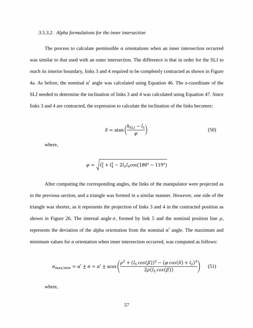
3.5.3.2. Alpha formulations for the inner intersection
The process to calculate permissible α orientations when an inner intersection occurred
was similar to that used with an outer intersection. The difference is that in order for the SLJ to
reach its interior boundary, links 3 and 4 required to be completely contracted as shown in Figure
4a. As before, the nominal α′ angle was calculated using Equation 46. The z-coordinate of the
SLJ needed to determine the inclination of links 3 and 4 was calculated using Equation 47. Since
links 3 and 4 are contracted, the expression to calculate the inclination of the links becomes:
𝛿 = atan �
ℎ𝑆𝐿𝐽 − 𝑙1𝜑
� (50)
where,
𝜑 = �𝑙32 + 𝑙42 − 2𝑙3𝑙4cos (180° − 119°)
After computing the corresponding angles, the links of the manipulator were projected as
in the previous section, and a triangle was formed in a similar manner. However, one side of the
triangle was shorter, as it represents the projection of links 3 and 4 in the contracted position as
shown in Figure 26. The internal angle 𝜎, formed by link 5 and the nominal position line 𝜌,
represents the deviation of the alpha orientation from the nominal α′ angle. The maximum and
minimum values for α orientation when inner intersection occurred, was computed as follows:
𝛼max/min = α′ ± σ = α′ ± acos�
𝜌2 + (𝑙5 𝑐𝑜𝑠(𝛽))2 − (𝜑 𝑐𝑜𝑠(𝛿) + 𝑙2)2
2𝜌(𝑙5 𝑐𝑜𝑠(𝛽)) � (51)
where,
57

𝜌 = �𝑝𝑥2 + 𝑝𝑦2
𝜑 = �𝑙32 + 𝑙42 − 2𝑙3𝑙4cos (180° − 119°)
Figure 26: Configuration with maximum alpha orientation and links 3 and 4 contracted
3.6. Collision-Free Path Planning
The main objective of this research was to move an object from an initial to a final
position. In order to do that, some algorithms (as the proposed by Zhang and Sobh [17]), base the
obstacle avoidance process on the manipulator configuration and keep the joints of the
manipulator away from the obstacle. These methods guarantee the avoidance of the obstacle, but
do not control the end-effector position and orientation. In this project a continuous collision-free
path was planned in the global coordinate system. Such path represents the movement of the end-
effector carrying the object from an initial to a final position and ensured that the object does not
collide with any stationary known obstacle. Under this scheme the position and orientation of the
58
tip of the manipulator was controlled as desired. Even though the joints of the manipulator were
not the main concern of the path planning algorithm, these were analyzed along the path to make
sure that none of them collide any obstacle. If any joint of the manipulator was found to be in a
collision path with an obstacle, the entire path is redesigned and verified again. All the steps
followed to plan a free-collision path are described in the following subsections.
Orientation of the end-effector was another important factor to consider when following
the path planned. Keeping the orientation constant is needed in special situations such as
handling containers carrying liquids. Since 𝛼 orientation was performed about the z-axis of the
global coordinate system, it did not tilt the end-effector. Therefore, any alpha angle could be
assigned by the path planning algorithm along the path. However, when beta or gamma
orientations were modified, the inclination of the end-effector was changed. Due to the limited
range of values for beta orientation computed by the dexterity analysis, finding suitable paths
and keeping beta orientation constant was difficult. When paths with constant beta orientation
were not found, the algorithm was capable of computing another path with slight change in the
beta orientation. Concerns about choosing the right gamma orientations were solved by keeping
it constant along the path.
3.6.1. Path Planning with Straight-Line
A straight line represented the simplest and shortest route when planning a path between
two points. Straight-line paths were the base for the path planning algorithm presented in this
project. There are two situations in which straight line paths were not followed: when the
manipulator end-effector had to cross the back or the center of the manipulator workspace, and
when an obstacle was on the straight line path. In the first case, via-points were added to ensure a
collision-free path between specific regions within the workspace. Via-points are intermediate
59

points through which the end-effector is forced to pass. An explanation is given later on how the
via-points are chosen. The via-points are connected by straight-line paths. Whenever the path
crosses an obstacle, such path was deformed by a virtual field that enclosed the obstacle. The
path modification is also explained later.
Before the algorithm creates a path, the initial and final points were verified to be inside
of the manipulator workspace. If they were not inside, the closest points inside the workspace are
suggested. The initial and final points were also checked to be outside the mobile robot base and
any obstacles. To design a straight-line path to connect the initial and final positions, or to
connect via-points, the algorithm linearly divided the differences between the X, Y, and Z
components of specified initial and final positions. A series of points called step-points were
obtained this way. The number of points computed was proportional to the distance between the
points to be connected. When performing tasks in which the control over the end-effector
manipulator was not crucial, the path was divided into a shorter number of step-points simulating
the Linear Joint Increment method (LJI) presented by Fotouhi et al [15]. The Linear End-
Effector Increment method (LEI) also presented in [15] was used when total control of the end-
effector was required; in this case the number of step-points chosen was substantially larger.
3.6.2. Straight-Line Path Deformation
Every obstacle located inside the workspace of the manipulator was modeled as a
rectangular prism. When crossing an obstacle, the straight path was modified by pushing the
points that were part of the path to a virtual boundary that enclosed the obstacle.
3.6.2.1. Ellipsoid Obstacle Enclosure
The virtual boundary enclosing the obstacle was assumed to have an ellipsoid shape. The
ellipsoid was modeled in the Cartesian coordinate system using the following equation [19]:
60

(𝑥 − 𝑥𝑐)2
𝑥𝑟2+
(𝑦 − 𝑦𝑐)2
𝑦𝑟2+
(𝑧 − 𝑧𝑐)2
𝑧𝑟2= 1 (52)
where,
𝑥𝑐,𝑦𝑐 , and 𝑧𝑐 are the Cartesian coordinates of the center of the ellipsoid and,
𝑥𝑟 ,𝑦𝑟 , and 𝑧𝑟 are the radius components of the ellipsoid as shown in Figure 27.
In order to totally enclose the obstacle, the center point of the ellipsoid was located at the
center point of the obstacle and the radius components were calculated large enough to cover the
entire obstacle as shown in Figure 27. Therefore, the boundary of the ellipsoid touched every
corner of the rectangular prism obstacle. The relation between the dimensions of the obstacle:
width (w), depth (d) and height (h), and the radius components of the ellipsoid: 𝑥𝑟 ,𝑦𝑟 , and 𝑧𝑟 are:
𝑥𝑟 =
𝑤cos(𝛽) cos(𝛼) , 𝑦𝑟 =
𝑑cos(𝛽) sin(𝛼) , 𝑧𝑟 =
ℎsin(𝛼) (53)
where,
𝛼 =𝜋4
, 𝛽 = atan(𝑐𝑜𝑠(𝛼))
Figure 27: Ellipsoid boundary enclosing a rectangular prism obstacle
61

3.6.2.2. Step-Points Repulsion
After computing the coordinate components of all step-points that were part of the
straight line path, each point was evaluated to determine if it was inside the virtual obstacle
boundary. This was achieved by substituting each point coordinates and each obstacle radius
components into Equation 52. If the result was higher than the unit, the specific step-point was
outside of the evaluated obstacle boundary; otherwise, if the result was less than the unit, the
step-point was inside the boundary and it was repelled. After all the step-points of the straight
line path were evaluated, a new non-linear collision-free path is formed as shown in Figure 28.
To determine in which direction the step-points were repelled, a unit vector was calculated by
computing the normal vector of a plane formed by the given initial and final positions and a
point located at the horizon: [∞, 0,0]. As shown, a 30mm thick safety zone was added to the
ellipsoid boundary to ensure total obstacle avoidance.
Figure 28: Step-points repulsion
62

3.6.3. Via-points Selection
Via-points are intermediate points located between the initial and final positions of the
end-effector, through which the tip of the manipulator is forced to pass to follow a desired path
[21]. Two regions presented difficulties when trying to cross them with the manipulator end-
effector: the center of the workspace, in which the base of the robot manipulator is mounted, and
the plane that connects regions A and G in Figure 29. The end-effector cannot cross this plane,
due to the limits of joint 𝜃𝜃1, therefore it has to travel around the center of the workspace. Via-
points are used to overcome those difficulties and such presented by the platform as it is too
large to be treated as a regular obstacle. The enclosed ellipsoid corresponding to the platform
would have significantly reduced the workspace of the manipulator. To avoid the
aforementioned problems the entire workspace of the manipulator was divided in seven regions
as shown in Figure 29. Four different via-points were selected inside the workspace to ensure
safety paths when crossing these regions. The seven regions are represented by letters (A, B, C,
D, E, F and G), and the four via points by numbers (1, 2, 3 and 4). The via-point coordinates are
shown in Table III. Such via-points can also be repelled by ordinary obstacle without
compromising the path planning. In order to cross from one specific region to another, more
than one via-point may be needed. The via-points were chosen according to the pattern presented
in Table IV.
Table III: Coordinate position of via-points
Via-point Cartesian coordinates (mm)
1 [−400 500 200]
2 [400 500 0]
3 [400 −500 0]
4 [−400 −500 200]
63

Table IV: Via-points selection pattern for region crossing safely
Departure region Destination region The required via-point number
A
B 1
C 1
D 1, 2
E 1, 2
F 1, 2, 3
G 1, 2, 3, 4
B
C None
D 2
E 2
F 2, 3
G 2, 3, 4
C
D None
E None
F 3
G 3, 4
D
E None
F 3
G 3, 4
E F None
G 4
F G 4
Note: The via-points required for traveling from X region to Y region are the same as those
required for traveling from Y region to X region. Where, X and Y can be any region
(A, B, C, D, E, F or G).
64

Figure 29: Via-point selection
Once the via-points were selected, straight-line paths to connect initial, final and via-
points positions are traced as before. The designed path is executed using the aforementioned
obstacle avoidance method. After defining admissible orientations along the path as discussed
before, every step-point is ready to be evaluated by the Iterative Inverse Kinematic method (IIK)
proposed. Finally, suitable joint configurations of the manipulators are obtained and used to
move the 6-DOF robot manipulator.
65

Chapter 4
Simulation and Experimental Results
4.1. Introduction
Simulation and experimental results were developed in two stages. The first stage
consisted of an evaluation of the Iterative Inverse Kinematics method (IIK) by performing three
predefined paths. The second stage probed the effectiveness of the entire path planning algorithm
by setting ten different scenarios with different number and pattern of obstacles. All these
obstacles have distinct dimensions and were placed in different locations. These ten scenarios
were representative samples of typical settings for the mobile robot and its manipulator. To
visually inspect the performance of these experiments a robotic simulator was used, in which the
6-DOF manipulator was modeled. The dimensions of the entire manipulator and its gripper end-
effector were considered. The description of the simulator and its graphic interface is shown in
Appendix F. For the second stage a computer program with friendly input user interface was
developed and it is presented in Appendix G. Such interface graphically acquired the dimensions
and location of obstacles in a similar way that a video camera would. It also considered the
location of the initial and final positions. The simulation and experimental results are presented
in the following sections.
4.2. Simulation Results (SR)
4.2.1. SR: Predefined Paths
The effectiveness of the IIK method proposed was verified by solving the inverse
kinematics problem for three different predefined paths. Each path corresponded to a particular
task of the robotic arm with the following scenarios: 1) moving the manipulator´s end-effector
66

from a height similar to that of an standard dining room table (0.8 m) to the top of the robot
platform (0.45 m), 2) from the ground floor to the top of the robot platform (0.45), and 3) from
the ground floor to the top of the table (0.8 m). To grasp and release objects properly, suitable
orientations at the beginning and at the end of each path were chosen. For each predefined path,
two via-points were added. Such via-points were specifically placed to avoid collision of the
end-effector with any stationary obstacles. The manipulator end-effector must pass through such
via-points to safely simulate obstacle avoidance. The segments that connect the initial point, the
via-points, and the final point were then divided into 39 steps each in order to cover a maximum
of 30 mm per step-point. The orientation of the three predefined paths was gradually modified at
each step. So, at the end of the path, the manipulator end-effector reached the desired final
orientation. Finally, at each step the IIK approach and the pseudo-inverse Newton’s method were
implemented for comparison to calculate the joint configurations.
When using the IIK method, several solutions may exist. A normalized parameter called
effort index (E) was used to pick the solution that represents the minimum joint angle changes.
Such index is of great importance during the inverse kinematics process since it aids to choose
the most efficient solution. This index was obtained by adding the absolute value of the
difference of every joint angle from step to step and then dividing the sum by the number of
joints as follows:
𝐸𝑖 =
∑ 𝑎𝑏𝑠�𝜃𝜃𝑛,𝑖 − 𝜃𝜃𝑛,𝑖−1�6𝑛=1
6 (54)
where,
𝑖 is the step number (𝑖 = 1,2,3, … , 39), and
𝑛 is the joint number (𝑛 = 1,2,3,4,5,6).
67

4.2.1.1. SR: The first predefined path
The first predefined path (table-top to robot-top) is shown in Figure 30. Straight-line path
between the first and second via-points was not implemented because reachable solutions were
not found with the orientations given. This problem was resolved by using an arc-path. Since the
Newton’s method converges to a solution close to the initial guess (in this case the solution of
the previous step), the joint configurations obtained by both methods (IIK and Newton) had
exactly the same values. The joint angles are presented in Figure 31. The normalized joint angle
effort (𝐸), required to move the manipulator from one step to the next was computed using
Equation 54; this index for this path is presented in Figure 32. Since the joint angles were almost
identical using both inverse kinematics methods (IIK and Newton), the joint displacement effort
graphs were also identical.
Figure 30: The first predefined path of the 6-DOF manipulator end-effector
68

Figure 31: Joint angles of the first predefined path using IIK method and Newton’s method
(the joint angles are identical in both methods)
Figure 32: The first predefined path joint effort index for IIK method and Newton’s
method (identical results)
69

The computational effort required for the two methods in order to solve the inverse
kinematics problem along the path was measured and it is shown in Figure 33. It is important to
recall that the IIK method can find up to 8 different solutions per position, meanwhile Newton’s
method using pseudo-inverse Jacobian only converges to one solution. Therefore, the index
presented in Figure 27 represents the CPU cycles required for each method per solution. Due to
the existence of an iterative process in both methods, a similar tolerance of convergence was
used (1 × 10⁻⁶ degrees).
Figure 33: The first predefined path computational efforts
4.2.1.2. SR: The second predefined path
For the second predefined path (ground-floor to robot-top), Figures 34 to 37 show the
representation of the path in the Cartesian coordinate system, the joint angular displacements, the
joint effort index and the computational effort index. Similarly to the first predefined path, an arc
route was used to connect the via-points in the second path due to the absence of solutions when
using a straight-line path.
70

Figure 34: The second predefined path of the 6-DOF manipulator end-effector
Figure 35: Joint angles of the second predefined path using IIK method and Newton’s
method (the joint angles are identical in both methods)
71

Figure 36: The second predefined path joint effort index for IIK method and Newton’s
method (identical results)
Figure 37: The second predefined path computational efforts
72

4.2.1.3. SR: The third predefined path
Figures 32 to 35 show the representation of the path in Cartesian coordinate system, the
joint angular displacement, the joint effort index, and the computational effort index for the third
predefined path (ground-floor to table-top).
Figure 38: The third predefined path of the 6-DOF manipulator end-effector
Figure 39: Joint angles of the third predefined path using IIK method and Newton’s
method (the joint angles are identical in both methods)
73

Figure 40: The third predefined path joint effort index for IIK method and Newton’s
method (identical results)
Figure 41: The third predefined path computational efforts
74

Finally, by conducting the aforementioned simulations, it was verified that the IIK
method proposed was capable of deriving multiple manipulator configurations when a solution
exists. Analyzing Figures 33, 37, and 41, it was proved that the computational efforts required
for solving the inverse kinematics using the IIK method were less than those required by the
pseudo-inverse Newton’s method per solution.
4.2.2. SR: Collision-Free Paths
The entire path planning method was verified by testing the algorithm using computer
simulation in ten different scenarios. These scenarios comprises several manipulator motion
situations: moving over one or several obstacles, moving over medium and large size obstacles,
moving among different regions as shown in Figure 29, and finally performing typical pick-and-
place operations by moving an object from one surface to another. The ten different scenarios are
shown in Figure 42. At each scenario every obstacle was modeled as a yellow rectangular prism.
The orange surface presented around each obstacle represents the ellipsoid enclosure that the
path repels to, and forms the collision-free path. The blue lines represent the manipulator several
instances of configurations along its path. A safety zone can be observed between the ellipsoid
boundary and the planned path at each scenario. As shown in Figure 42e two via-points were
chosen by the path planning algorithm to avoid manipulator motion conflict zones as explained
previously in Chapter 3. The joint angles were plotted at this stage to inspect the planned path
from step-point to step-point and ensure smooth transitions. The joint angles of a representative
pick-and-place operation (Figure 42j) were presented in Figure 43. As before the motion
normalized effort index required for the manipulator, was computed using Equation 54 and it is
shown in Figure 44. The angular velocity chose for the 6-DOF manipulator is proportional to the
joint effort index obtained.
75

(a)
(b)
(c)
(d)
(e)
(f)
76

(g)
(h)
(i)
(j)
Figure 42: Pick-and-place operations with obstacle avoidance for ten scenarios: a) Over an
obstacle; b) Across an obstacle; c) Over two obstacles; d) Across two obstacles; e) Through
different regions; f) Over a big obstacle; g) From the top of the robot platform to the top of
a table; h) From the top of one obstacle to another; i) From the top of the robot platform to
the top of a table; j) From the top of one table to another while avoiding an obstacle
77

Figure 43: The 6-DOF Manipulator joint angles of the path shown in Figure 42j
Figure 44: Joint effort index of the path shown in Figure 42j
The joint angle plots and the normalized effort index plots for the remaining paths are
presented in Appendix H.
78

4.3. Experimental Results (ER)
After validating the IIK method and the path planning algorithm performances using the
robotic simulator, experiments were conducted on the actual 6-DOF robot manipulator. Each
scenario was properly set (Figure 45) to mimic the simulations presented in Section 4.1. As
shown in Appendix A, the functionality of the operational commands for the manipulator
provided by the manufacturer is limited. The most appropriate function that accurately follows
the path is the constant velocity based motion. This function receives the desired goal position
and time, and computes the constant velocity required to perform the task. When plugging the
manipulator configurations from each step-point one-by-one directly into the program, undesired
vibrations were detected. This was caused by the stoppage of motion at each step-point inherent
to the program functionality. These problems were solved by sending the command in progress
after the 95% of the total time required by the previous command had been consumed. This
updating procedure solved the vibration problem but added some error in the end-effector
position during the manipulator motion.
To compare experimental and simulation results, experimental data was directly obtained
from the 6-DOF manipulator using the functions provided by the manufacturer presented in
Appendix A. The joint angles, the joint velocities and the electrical current consumption are
some of the parameters acquired in each experiment. Visual inspections were performed to
ensure the manipulator would not collide with any obstacle; however, such inspections are
insufficient when small errors occur. As the Cartesian position of the end-effector is hard to
measure in a three dimensional space when the manipulator is in motion, it was calculated by
inputting the obtained experimental joint angles into the forward kinematics expression
(Equation 4) presented in section 3.2.
79

Figure 45: Preparation of an experimental scenario
4.3.1. ER: Positioning error on predefined paths
After plotting the joint angles and the end-effector positions using the experimental
results obtained in the predefined paths, the graphs were found to be similar to those presented in
Section 4.2.1 (Figures 30, 31, 34, 35, 38 and 39). Even when no significant differences were
observed in those graphs, small deviations exist. The joint difference between the theoretical and
the experimental results for the predefined paths 1, 2 and 3 are shown in Figures 46, 48 and 50
respectively. The positioning error of the predefined paths 1, 2 and 3 are presented in Figure 47,
49 and 51, respectively. Since the maximum end-effector distance error presented in the three
predefined paths was not bigger than 10 mm, this distance was chosen as the minimum longitude
for the safety zone (Figure 28) on the predefined path experiments.
80

Figure 46: Analytical versus experimental joint error for the first predefined path
Figure 47: Positioning error between analytical and experimental results for the end-
effector for the first predefined path
81

Figure 48: Analytical versus experimental joint error for the second predefined path
Figure 49: Positioning error between analytical and experimental results for the end-
effector for the second predefined path
82

Figure 50: Analytical versus experimental joint error for the third predefined path
Figure 51: Positioning error between analytical and experimental results for the end-
effector for the third predefined path
83
4.3.2. ER: Positioning error using the path planning algorithm
Updating the motion commands before a step was completed also affected the path
planning algorithm. The error analysis (comparing simulation and experimental results) was
performed for the ten aforementioned scenarios in a similar manner as the predefined paths.
After plotting the joint angles and the end-effector positions using the experimental results
obtained by following the paths planned on the ten scenarios, the graphs were similar to those
presented in Section 4.2.2 (Figures 43 and 44). As for the predefined path, errors exist even
though no significant differences were observed. The joint angle error and the positioning error
of the end-effector presented between simulation and experimental results of a representative
path are shown in Figures 52 and 53 respectively. Simulation and experimental results
comparison for the remaining paths are presented in Appendix I. A summary of the positioning
displacement error graphs that contains the mean error and the maximum error for each scenario
is presented in Figure 54. The mean values of the error alone are also presented for clarification
in Figure 55.
Additionally; the velocity of each joint of the actual manipulator at every step-point was
plotted using a function (PCube_getVel), which calculates the actual velocity of the manipulator
using the incremental encoder attached to each module of the manipulator. The angular velocity
of the manipulator joints for a representative path for the ten different scenarios is shown in
Figure 56. The abruptly change of angular velocity on some joints did not present difficulties in
the manipulator motion. The angular velocity graphs obtained for the remaining paths are also
shown in Appendix I.
84

Figure 52: Analytical versus experimental joint error for path shown in Figure 42j
Figure 53: Positioning error between analytical and experimental results for the end-
effector for the path shown in Figure 42j
85

Figure 54: Summary of the mean error and the maximum error for ten different scenarios
Figure 55: Summary of the mean error for ten different scenarios
86

Figure 56: Experimental joint velocity of the path shown in Figure 42j
As shown in Figures 47, 49, 51 and 53, the positioning error of the end-effector of the
manipulator at the beginning and at the end of each path is zero. The same behaviour was
observed in the path planning algorithm graphs. This means that the manipulator accuracy was
not compromised by performing an early command update. The maximum error results obtained
from the summary of the error graphs (Figures 54 and 55) suggest a minimum safety zone of
30mm when the manipulator is in motion. Even when the maximum error in motion was high,
the mean error remained low for each path. Finally, a sequence of pictures is shown in Figure 57
to illustrate the path planning operation of a representative path using the 6-DOF manipulator.
The yellow boxes represent the obstacles used in the different experimental scenarios. The
sequence shows the initial, intermediate and final positions of the manipulator during pick-and-
place operations. The obstacle avoidance process is also shown in Figure 57.
87

(a)
(b)
(c)
(d)
Figure 57: Sequence of path experiment shown in Figure 42j: a) Robot and obstacle
settings; b) Picking the object; c) Obstacle avoidance; d) Placing the object
88
Chapter 5
Conclusions
5.1 Summary
In this thesis, several methods were implemented to make a 6-DOF manipulator capable
of performing pick-and-place operations. Some of these methods were used to achieve specific
tasks such as: solving the inverse kinematics problem or planning a collision-free path. Some
other methods such as forward kinematics description, workspace evaluation and dexterity
analysis, were used to describe the manipulator and its capabilities. Each of these methods were
modified and implemented in a 6-DOF manipulator attached to a wheeled mobile robot. The
manipulator was accurately described by obtaining the link transformation matrices from each
joint using the Denavit-Hartenberg (DH) notations. An Iterative Inverse Kinematics method
(IIK) was used to find multiple configurations for the manipulator along a given path. The IIK
method was based on the specific geometric characteristic of the manipulator, in which several
joints share a common plane. In order to calculate the first two joint angles of the manipulator,
two non-linear trigonometric equations were derived and solved using a bisectional method. The
remaining angles which are functions of the two known angles were computed using kinematic
expressions. In order to find admissible solutions along the path, the workspace of the
manipulator was considered. Algebraic formulations, to obtain the specific workspace of the 6-
DOF manipulator on the Cartesian coordinate space, were derived from the singular
configurations of the manipulator. Local dexterity analysis was also needed in order to know
possible orientations of the end-effector for specific Cartesian coordinate positions. The closed-
form expressions for the range of such orientations (alpha, beta and gamma) were derived by
89

adapting an existing dexterity method. Two methods were implemented to plan the free-collision
path needed to move an object from one place to another without colliding with an obstacle. Via-
points were added in order to avoid the robot mobile platform and the zones in which the
manipulator showed motion difficulties. Finally, the segments located between initial, final, and
via-points positions, were connected using straight lines forming a global path. To form the
collision-free path, the straight-line paths were modified to avoid the obstacles that intersected
the path.
5.2 Conclusions
After analyzing the overall performance of the proposed algorithm, and comparing the
simulation and experimental results, the following conclusions were established:
• The joint angles of the manipulator were successfully calculated at each position along
the predefined paths using the IIK introduced here. The performance of this method was
verified by obtaining all possible solutions for each specific position of the end-effector.
Such property allowed the manipulator to choose a feasible solution to avoid obstacles.
The IIK method proved to be a suitable method for solving the Inverse Kinematics
problem.
• The performance of the IIK method was compared with the performance of the pseudo-
inverse Newton’s method. The computational efforts per solution required to solve the
joint angles using the IIK method were less than those required by the pseudo-inverse
Newton’s method.
90

• The analysis of the workspace boundaries allowed for the identification of the reachable
points of the end-effector for the selection of the most appropriate path. Even though
most of the parametric surfaces computed for the 6-DOF manipulator, do not constitute a
boundary for the workspace, they must be avoided as they caused motion difficulties in
the manipulator.
• The algorithm presented here, was capable of recognizing whether a given position was
inside of the workspace of the manipulator or not, during every trial. The tests showed
that the implementation of the proposed workspace analysis, accurately describes the
boundaries of the robot manipulator in the robot task space, Cartesian coordinate system.
• Using local dexterity analysis, at least one solution was obtained at any position located
inside of the workspace of the manipulator when suitable orientations were chosen.
Knowing the permissible orientations of the end-effector at any position of the
manipulator is a critical parameter when determining the end-effector position. The
correct selection of these parameters guarantees the convergence of the inverse
kinematics problem.
• The obstacle avoidance process was verified by performing a visual inspection of the 6-
DOF manipulator motion produced by the path planning algorithm, in ten different
scenarios. The smooth transitions observed in the joint angular displacement and velocity
graphs, confirmed that the manipulator is capable of avoiding obstacles carefully and
with minimum vibration.
91

• Although this project focused on a particular robotic arm, the principles and methods
described in this thesis may be of great interest to engineers and programmers
implementing kinematic methods in manipulators with similar characteristics.
5.3 Recommendations for future research
Valuable conclusions were obtained from this research. To improve the overall
performance of the proposed algorithm, some feature works are suggested. The following are
recommendations for future research:
1) To work with mobile obstacles, where real time visual recognition of the environment is
required. The implementation of a device capable of mapping the obstacles dimensions and
positions can replace the existing obstacle selection function.
2) The evaluation of the end-effector orientation when approaching an obstacle can be improved
to properly grasp an object if the specific dimensions and properties are known.
3) The implementation of image processing combined with voice recognition techniques can be
implemented to create an intelligent system capable of receiving, processing and executing
commands for objects handling by the 6-DOF manipulator.
4) The integration of the manipulator functions and the mobile robot navigation will allow for
the execution of tasks of increased complexity.
92

References
[1] J. Denavit and R. S. Hartenberg, “A Kinematic Notation for Lower-Pair Mechanisms
based on Matrices”, Journal of Applied Mechanics, Vol. 23, pp. 215-221, June 1955.
[2] J. J. Craig, “Introduction to Robotics: Mechanics and Control”, 3rd edition, Prentice Hall,
Upper Saddle River, N.J., USA, 2005.
[3] I. A. Vasilyev and A. M. Lyashin, “Analytical Solution to Inverse Kinematics Problem
for 6-DOF Robot-Manipulator”, Automation and Remote Control, Vol. 71, No. 10, pp.
2195-2199, 2010.
[4] M. Shimizu, H. Kakuya, W. K. Yoon, K. Kitagaki and K. Kosuge, “Analytical Inverse
Kinematic Computation for 7-DOF Redundant Manipulators With Joint Limits and Its
Application to Redundancy Resolution”, IEEE Transactions on Robotics, Vol. 24, No. 5,
pp. 1131-1142, 2008.
[5] C. W. Wampler, “Manipulator Inverse Kinematics Solution Based on Vector
Formulations and Damped Least Squares Methods”, IEEE Transactions on Systems,
Man, and Cybernetics, Vol. 16, No. 1, pp. 93-101, 1986.
[6] S. R. Buss, J. S. Kim, “Selectively Damped Least Squares for Inverse Kinematics”,
Journal of Graphics Tools, Vol. 10, No. 3, pp. 37-49, 2005.
[7] G. Z. Grudic and P. D. Lawrence, “Iterative Inverse Kinematics with Manipulator
Configuration Control”, IEEE Transactions on Robotics and Automation, Vol. 9, No. 4,
August 1993.
93

[8] D. Pieper and B. Roth, “The Kinematics of Manipulators Under Computer Control”,
Proceedings of the Second International Congress of Theory of Machines and
Mechanisms, Zacopane, Poland, Vol. 2, pp. 159-169, 1969.
[9] B. Siciliano, “A Closed-Loop Inverse Kinematic Scheme for Online Joint-Based Robot
Control”, Robotica, Vol. 8, No. 3, pp. 231-243, 1990.
[10] K. Abdel-Malek, H. Yeh and S. Othman, “Interior and Exterior Boundaries to the
Workspace of Mechanical Manipulators”, Robotics and Computer Integrated
Manufacturing, Vol. 16, No. 5, pp. 365-376, 2000.
[11] K. Abdel-Malek and H. Yeh, “Analytical Boundary of the Workspace for General 3-DOF
Mechanisms”, International Journal of Robotic Research, Vol. 16, No. 2, pp. 198-213,
1997.
[12] K. Abdel-Malek and H. Yeh, “Geometric Representation of the Swept Volume using
Jacobian Rank-Deficiency Conditions”, Computer Aided Design, Vol. 29, No. 6, pp. 457-
468, 1997.
[13] Niku, S., “Introduction to Robotics: Analysis, Systems, Applications”, Prentice Hall,
New Jersey, USA, 2001.
[14] K. Abdel-Malek and H. Yeh, “Local Dexterity Analysis for Open Kinematic Chains”,
Mechanism and Machine Theory, Vol. 35, No. 1, pp. 131-154, 2000.
[15] R. Fotouhi, H. Salmasi, I. Vaheed and M. Vakil, “Trajectory Planning for a Wheeled
Mobile Robot and its Robotic Arm”, Proceedings of ASME 2010, International
94

Mechanical Engineering Congress & Exposition, Vancouver, BC, Canada, November 12-
18, 2010.
[16] G. Ping, B. Wei, X. Li, X. Luo, “Real Time Obstacle Avoidance for Redundant Robot”,
Proceedings of the 2009 IEEE, International Conference on Mechatronics and
Automation, August 9-12, Changchun, China, pp. 223-228, 2009.
[17] W. Zhang and T. M. Sobh, “Obstacle Avoidance for Manipulators”, Systems Analysis
Modelling Simulation, Vol. 43, No. 1, pp. 67-74, January 2003.
[18] Chien-Chou Lin, “A Hierarchical Path Planning of Manipulators Using Memetic
Algorithm”, Proceedings of the 2009 IEEE, International Conference on Information and
Automation, June 22-25, Zhuhai/Macau, China, 2009.
[19] MathWorks®, Matlab® – Documentation Center (on-line): Surfaces, Volumes and
Polygons: ellipsoid, Version 7.10 (R2010a), 2010.
[20] Schunk®, Amtec Robotics – Programmers guide for PowerCube™, Version 1.3, 2007.
[21] McGraw-Hill Professional, “McGraw-Hill Dictionary of Scientific and Technical
Terms”, 6th edition, McGraw-Hill, New York, USA, 2002.
[22] RoboWorks™, 3D Robot Modeling Software – Demonstration Version 3.0
http://www.newtonium.com/, January 7th 2012.
95

Appendix A
Operational functions of the 6-DOF manipulator
This appendix shows the description of the commands implemented in the algorithm
proposed in this thesis. These commands were selected from the programming guide [19]
provided by the manipulator manufacturer.
Table V: List of implemented commands of the 6-DOF manipulator
Function Description
PCube_openDevice Opens the interface by specifying an initial string. Result is a valid
device ID
PCube_closeDevice Closes the interface by specifying the device ID
PCube_getPos
Retrieves the actual module position by specifying the device ID and a
module ID. Result is the position in radians
PCube_getVel
Retrieves the speed of joint by specifying the device ID and a module ID.
Result is the real speed in rad/s
PCube_getCur
Retrieves the actual current information by specifying the device ID and
a module ID. Result is the actual current in A
PCube_setMaxVel
Sets the maximum speed of a joint by specifying the device ID, a module
ID and the new value in rad/s
PCube_setMaxCur
Sets the actual maximum current by specifying the device ID, a module
ID and the new maximum current in A
PCube_homeModule Starts a homing procedure which consists of moving a module to its
initial position by specifying the device ID and the module ID
96

PCube_homeAll Starts a homing procedure of all modules connected to the bus. All
modules are moved to its initial position
PCube_moveRamp
Starts a ramp motion profile of the module specified by device ID and
module ID. The target position is given in radians, the target speed in
rad/s and the target acceleration in rad/s²
PCube_moveStep
Starts motion to the target position specified in radians. Target time for
the ride is specified in ms
PCube_moveVel Starts a constant speed motion of a joint. This command modifies the
current applied to the joint if the payload decreases or increases in order
to keep the speed of the joint constant. Target speed is specified in rad/s
PCube_moveCur Starts a constant current motion of a joint. This command keeps the
speed of the joint constant no matter what the payload is. The target
current is specified in A
97

Appendix B
Link transformations matrices of the 6-DOF manipulator
Original transformations obtained following Craig’s convention [2] implemented in Equation 4:
𝑇10 = �
𝑐1 −𝑠1 0 0𝑠1 𝑐1 0 00 0 1 𝑙10 0 0 1
� 𝑇21 = �
𝑐2 −𝑠2 0 𝑙20 0 1 0−𝑠2 −𝑐2 0 0
0 0 0 1
�
𝑇32 = �
𝑐3 −𝑠3 0 00 0 1 𝑙3−𝑠3 −𝑐3 0 0
0 0 0 1
� 𝑇43 = �
𝑐4 −𝑠4 0 00 0 1 0−𝑠4 −𝑐4 0 0
0 0 0 1
�
𝑇54 = �
𝑐5 −𝑠5 0 𝑙4𝑠5 𝑐5 0 00 0 1 00 0 0 1
� 𝑇65 = �
𝑐6 −𝑠6 0 00 0 1 𝑙5−𝑠6 −𝑐6 0 0
0 0 0 1
�
Modified transformations to establish home position (Figure 8) as initial position, in which all
the joint angles are equal to zero:
𝑇10 = �
𝑐1 −𝑠1 0 0𝑠1 𝑐1 0 00 0 1 𝑙10 0 0 1
� 𝑇21 = �
𝑠2 𝑐2 0 𝑙20 0 1 0𝑐2 −𝑠2 0 00 0 0 1
�
𝑇32 = �
𝑐3 −𝑠3 0 00 0 1 𝑙3−𝑠3 𝑐3 0 0
0 0 0 1
� 𝑇43 = �
𝑠4 𝑐4 0 00 0 1 0𝑐4 −𝑠4 0 00 0 0 1
�
𝑇54 = �
−𝑠5 −𝑐5 0 𝑙4𝑐5 −𝑠5 0 00 0 1 00 0 0 1
� 𝑇65 = �
𝑐6 −𝑠6 0 00 0 1 𝑙5−𝑠6 𝑐6 0 0
0 0 0 1
�
98

Appendix C
Computation of the Jacobian matrix of the 6-DOF manipulator
The global position vector (𝐺𝜃) of the end-effector of the 6-DOF manipulator was
computed as:
𝐺𝜃 = �
𝑝𝑥𝑝𝑦𝑝𝑧� = �
𝑓1(𝜃𝜃1, 𝜃𝜃2, 𝜃𝜃3, 𝜃𝜃4,𝜃𝜃5)𝑓2(𝜃𝜃1,𝜃𝜃2,𝜃𝜃3,𝜃𝜃4,𝜃𝜃5)𝑓3(𝜃𝜃2,𝜃𝜃3,𝜃𝜃4,𝜃𝜃5)
� (55)
where,
�𝑓1(𝜃𝜃1,𝜃𝜃2,𝜃𝜃3,𝜃𝜃4, 𝜃𝜃5)𝑓2(𝜃𝜃1,𝜃𝜃2,𝜃𝜃3,𝜃𝜃4, 𝜃𝜃5)𝑓3(𝜃𝜃2,𝜃𝜃3,𝜃𝜃4, 𝜃𝜃5)
� = �𝑙2𝑐1 + 𝑙3𝑐1𝑐2 + (𝑙5𝑠45 + 𝑙4𝑠4)(𝑠1𝑠3 + 𝑐1𝑠2𝑐3) + (𝑙5𝑐45 + 𝑙4𝑐4)(𝑐1𝑐2)𝑙2𝑠1 + 𝑙3𝑠1𝑐2 − (𝑙5𝑠45 + 𝑙4𝑠4)(𝑐1𝑠3 − 𝑠1𝑠2𝑐3) + (𝑙5𝑐45 + 𝑙4𝑐4)(𝑠1𝑐2)
𝑙5(𝑠45𝑐2𝑐3 − 𝑐45𝑠2) + 𝑙4(𝑐2𝑐3𝑠4 − 𝑐4𝑠2) − 𝑙3𝑠2 + 𝑙1�
Then the Jacobian matrix (𝐽𝜃) can be obtained by taking the partial derivative of each
element from the global position vector (Gθ) with respect to each joint variable as:
𝐽𝜃 =
⎣⎢⎢⎢⎢⎢⎡𝜕𝑓1𝜕𝜃𝜃1
𝜕𝑓1𝜕𝜃𝜃2
𝜕𝑓1𝜕𝜃𝜃3
𝜕𝑓1𝜕𝜃𝜃4
𝜕𝑓1𝜕𝜃𝜃5
𝜕𝑓2𝜕𝜃𝜃1
𝜕𝑓2𝜕𝜃𝜃2
𝜕𝑓2𝜕𝜃𝜃3
𝜕𝑓2𝜕𝜃𝜃4
𝜕𝑓2𝜕𝜃𝜃5
𝜕𝑓3𝜕𝜃𝜃1
𝜕𝑓3𝜕𝜃𝜃2
𝜕𝑓3𝜕𝜃𝜃3
𝜕𝑓3𝜕𝜃𝜃4
𝜕𝑓3𝜕𝜃𝜃5⎦
⎥⎥⎥⎥⎥⎤
(56)
where,
𝜕𝑓1𝜕𝜃𝜃1
= −𝑙2𝑠1 − 𝑙3𝑠1𝑐2 + (𝑙5𝑠45 + 𝑙4𝑠4)(𝑐1𝑠3 − 𝑠1𝑠2𝑐3) − (𝑙5𝑐45 + 𝑙4𝑐4)(𝑠1𝑐2)
𝜕𝑓1𝜕𝜃𝜃2
= −𝑙3𝑐1𝑠2 + (𝑙5𝑠45 + 𝑙4𝑠4)(𝑐1𝑐2𝑐3) − (𝑙5𝑐45 + 𝑙4𝑐4)(𝑐1𝑠2)
𝜕𝑓1𝜕𝜃𝜃3
= (𝑙5𝑠45 + 𝑙4𝑠4)(𝑠1𝑐3 − 𝑐1𝑠2𝑠3)
99

𝜕𝑓1𝜕𝜃𝜃4
= (𝑙5𝑐45 + 𝑙4𝑐4)(𝑠1𝑠3 + 𝑐1𝑠2𝑐3) − (𝑙5𝑠45 + 𝑙4𝑠4)(𝑐1𝑐2)
𝜕𝑓1𝜕𝜃𝜃5
= (𝑙5𝑐45)(𝑠1𝑠3 + 𝑐1𝑠2𝑐3)− 𝑙5𝑐1𝑐2𝑠45
𝜕𝑓2𝜕𝜃𝜃1
= 𝑙2𝑐1 + 𝑙3𝑐1𝑐2 + (𝑙5𝑠45 + 𝑙4𝑠4)(𝑠1𝑠3 + 𝑐1𝑠2𝑐3) + (𝑙5𝑐45 + 𝑙4𝑐4)(𝑐1𝑐2)
𝜕𝑓2𝜕𝜃𝜃2
= −𝑙3𝑠1𝑠2 + (𝑙5𝑠45 + 𝑙4𝑠4)(𝑠1𝑐2𝑐3) − (𝑙5𝑐45 + 𝑙4𝑐4)(𝑠1𝑠2)
𝜕𝑓2𝜕𝜃𝜃3
= −(𝑙5𝑠45 + 𝑙4𝑠4)(𝑐1𝑐3 + 𝑠1𝑠2𝑠3)
𝜕𝑓2𝜕𝜃𝜃4
= −(𝑙5𝑐45 + 𝑙4𝑐4)(𝑐1𝑠3 − 𝑠1𝑠2𝑐3) − (𝑙5𝑠45 + 𝑙4𝑠4)(𝑠1𝑐2)
𝜕𝑓2𝜕𝜃𝜃5
= −(𝑙5𝑐45)(𝑐1𝑠3 − 𝑠1𝑠2𝑐3) − 𝑙5𝑠1𝑐2𝑠45
𝜕𝑓3𝜕𝜃𝜃1
= 0
𝜕𝑓3𝜕𝜃𝜃2
= −𝑙5(𝑠45𝑠2𝑐3 + 𝑐45𝑐2) − 𝑙4(𝑠2𝑐3𝑠4 + 𝑐4𝑐2) − 𝑙3𝑐2
𝜕𝑓3𝜕𝜃𝜃3
= −𝑙5𝑠45𝑐2𝑠3 − 𝑙4𝑐2𝑠3𝑠4
𝜕𝑓3𝜕𝜃𝜃4
= 𝑙5(𝑐45𝑐2𝑐3 + 𝑠45𝑠2) + 𝑙4(𝑐2𝑐3𝑐4 + 𝑠4𝑠2)
𝜕𝑓3𝜕𝜃𝜃5
= 𝑙5(𝑐45𝑐2𝑐3 + 𝑠45𝑠2)
100

Appendix D
Singularity sets of the 6-DOF manipulator
According to Abdel-Malek and Yeh [12] there are three types of singularities: rank-
deficiency singularity set, rank-deficiency of the reduced-order accessible set, and constraint
singularity set. The proper methodology to identify these singularity sets is explained in [12].
Table VI: Type I and type II singularity sets
Singularity category Set 𝜽𝟏 𝜽𝟐 𝜽𝟑 𝜽𝟒 𝜽𝟓 Type I 𝑠(1) variable variable NA 0° 0°
Type II
𝑠(2) -160° variable
90°
variable
0° 𝑠(3) 160° 90° 0° 𝑠(4) -160° -120°
variable
0° 𝑠(5) -160° 95° 0° 𝑠(6) 160° -120° 0° 𝑠(7) 160° 95° 0° 𝑠(8) -160°
variable
-160° 0° 𝑠(9) -160° 160° 0° 𝑠(10) 160° -160° 0° 𝑠(11) 160° 160° 0° 𝑠(12) -160° -90° -119°
variable
𝑠(13) -160° 90° -119° 𝑠(14) 160° -90° -119° 𝑠(15) 160° 90° -119° 𝑠(16) -160° -90° 119° 𝑠(17) -160° 90° 119° 𝑠(18) 160° -90° 119° 𝑠(19) 160° 90° 119° 𝑠(20)
variable
-120° -160°
variable
0° 𝑠(21) -120° 160° 0° 𝑠(22) 95° -160° 0° 𝑠(23) 95° 160° 0° 𝑠(24) -120° 0° -119°
variable 𝑠(25) -120° 0° 119° 𝑠(26) 95° 0° -119° 𝑠(27) 95° 0° 119°
101

Singularity category Set 𝜽𝟏 𝜽𝟐 𝜽𝟑 𝜽𝟒 𝜽𝟓
Type II
𝑠(28)
variable
-120° 0°
variable
-119° 𝑠(29) -120° 0° 119° 𝑠(30) 95° 0° -119° 𝑠(31) 95° 0° 119° 𝑠(32)
variable
0° -119° -119° 𝑠(33) -90° -119° -119° 𝑠(34) -90° -119° -119° 𝑠(35) 0° -119° 119° 𝑠(36) -90° -119° 119° 𝑠(37) 90° -119° 119°
Type III Singularity set
The singularity sets of the third type are composed by the eight combinations formed
with the three non-variable joint angles limits as defined in the following table:
Table VII: Type III singularity set
Set 𝜽𝟏 𝜽𝟐 𝜽𝟑 𝜽𝟒 𝜽𝟓 𝑠(38) to 𝑠(45) -160° 160° -120° 95° -160° 160° variable Variable 𝑠(46) to 𝑠(53) -160° 160° -120° 95° Variable -119° 119° 𝑠(54) to 𝑠(61) -160° 160° -120° 95° Variable -119° 119° 𝑠(62) to 𝑠(69) Variable
-120° 95° -160° 160° -119° 119° Variable 𝑠(70) to 𝑠(77)
variable
-160° 160° -119° 119° -119° 119° 𝑠(78) to 𝑠(85) -160° 160° -160° 160° Variable -119° 119° 𝑠(86) to 𝑠(93) -160° 160° -160° 160° -119° 119° Variable 𝑠(94) to 𝑠(101) -160° 160° variable Variable -119° 119° 𝑠(102)to 𝑠(109) variable -120° 95° -160° 160° -119° 119° 𝑠(110)to 𝑠(117) -120° 95° variable -119° 119° -119° 119°
102

Appendix E
Analysis of admissible normal acceleration motion of specific points located over singular
parametric surfaces
In this Appendix, the analytical solution for the normal acceleration motion of specific
points located over the singular parametric considered in Section 3.4.3 is presented. The
formulations presented by Abdel-Malek in [10] are also summarized.
Normal acceleration motion analysis
Any point located in a singular surface allows motion normal to the surface in either
direction depending on the difference in the acceleration (defined by 𝜂) such that:
𝜂 = 𝑎𝑛 −
𝑣𝑡2
𝜌0 (57)
where, 𝑣𝑡 is the tangential velocity, 𝑎𝑛 is the normal acceleration, and 1 𝜌0⁄ is the normal
curvature of the singular surface.
To include limits of the joints in the previous formulation, parameterization of the joint
variables is needed. The joint constraints are parameterized as:
𝑞𝑖(𝜆𝑖) =
(𝑞𝑖𝑈 + 𝑞𝑖𝐿)2
+(𝑞𝑖𝑈 − 𝑞𝑖𝐿)
2sin (𝜆𝑖) (58)
where, 𝑞𝑖 = 𝜃𝜃𝑖, 𝑞𝑖𝑈 and 𝑞𝑖𝐿 are the upper and lower limits of the joint. New parameters were
introduced such that 𝑞 = 𝑞(𝑠), where 𝑠 = [𝜆1, 𝜆2, … 𝜆𝑛]𝑇. Now the joint limits can be obtained
by varying the new parameters 𝜆𝑖 between −𝜋 2⁄ and 𝜋 2⁄ .
103

The first step when calculating the acceleration motion is to obtain the normal vector
(𝑁0𝑇) to the parametric surface by:
𝑁0𝑇 = 𝑛𝑢𝑙𝑙 �𝐺𝑞 �𝑞0(𝑠𝑖)� 𝑞𝑠 �𝑠0
(𝑠𝑖)��𝑇 (59)
where 𝐺𝑞 = 𝜕𝐺 𝜕𝑞⁄ , 𝑞0(𝑠𝑖) is the joints configuration of the point to evaluate over the singular
surface, and 𝑠0(𝑠𝑖) is the parametrized joints configuration of the same point. The function 𝑛𝑢𝑙𝑙
finds the vector or vectors which multiplied by the evaluated term equals zero.
The component of the normal configuration, in matrix form, is written as:
𝑎𝑛 = �̇�𝑇𝐻∗�̇� (60)
where,
𝐻∗(𝑞0, 𝑠0) = 𝑞𝑠𝑇[𝑁0𝑇𝐺]𝑞𝑞𝑞𝑠 + �
𝑑(𝑁0𝑇𝐺)𝑑𝑞𝑖
∙ [𝑞𝑖]𝑠𝑠
𝑛
𝑖=1
(61)
where, 𝑞𝑠 = 𝜕𝑞 𝜕𝑠⁄ , and [𝑁0𝑇𝐺]𝑞𝑞 = 𝜕2(𝑁0𝑇𝐺) 𝜕𝑞2⁄
The component of the tangential velocity over the normal curvature is defined in a matrix
form as:
𝑣𝑡2
𝜌0= �̇�𝑇𝑞𝑠𝑇𝐺𝑞𝑇𝐵𝑇[𝑁0𝑇𝑓]𝑢𝑢𝐵𝐺𝑞𝑞𝑠�̇� (62)
where 𝑢 = �𝑞𝑖, 𝑞𝑗�𝑇are the remaining joints variables which are not fixed, 𝑓 is the singular
parametric entity, and the generalized inverse (𝐵) is evaluated as:
104

𝐵 = [𝐸𝑓𝑢]−1𝐸 (63)
where E is defined as:
𝐸 = �1 0 00 1 0� if the first and second rows of 𝑓𝑢 are independent,
𝐸 = �1 0 00 0 1� if the first and third rows of 𝑓𝑢 are independent,
𝐸 = �0 1 00 0 1� if the second and third rows of 𝑓𝑢 are independent.
In order to obtain the normal acceleration, Equations 60 and 62 are substituted in
Equation 57:
𝜂 = 𝑎𝑛 −
𝑣𝑡2
𝜌0= �̇�𝑇𝑄∗�̇� (64)
where,
𝑄∗ = 𝐻∗ − 𝑞𝑠𝑇𝐺𝑞𝑇𝐵𝑇[𝑁0𝑇𝑓]𝑢𝑢𝐵𝐺𝑞𝑞𝑠 (65)
From Equation 65, 𝑄∗ is a quadratic form that defines whether the acceleration motion is
in the direction of the normal vector or in the opposite direction. By computing the eigenvalues,
the direction of 𝑄∗(positive or negative), can be determined. If all the eigenvalues are positive,
the singular surface admits motion in the direction of the normal vector at the evaluated point.
On the other hand, if the eigenvalues are negative, the movement allowed by the singular surface
is in the opposite direction to the normal vector. The previous analysis is valid only when 𝑞𝑖 is
not at a limit, otherwise 𝑄∗ yields to a semi-definite quadratic form. If 𝑄∗ is indefinite (the
105

eigenvalues are positive and negative), the singular surface admits motion in any direction and
the surface is not a boundary.
According to Abdel-Malek [10], when a joint is at its limit, its parameterized form
equates to zero and Q∗ becomes semi-definite. In order to determine the direction of the motion,
an additional parameter must be evaluated:
𝜎 = 𝑁0𝑇𝐺𝑞𝑖𝛿𝑞𝑖 (66)
where,
𝛿𝑞𝑖 = �+1 if 𝑞𝑖 is at lower limit −1 if 𝑞𝑖 is at upper limit (67)
If Equation 66 evaluates to zero because N0T is perpendicular to Gqi, evaluating
the sign of the difference in the normal curvature (K�) is needed.
𝐾� = 𝐺𝑞𝑖𝑇 𝐵𝑇[𝑁0𝑇𝐺]𝑢𝑢𝐵𝐺𝑞𝑖 − [𝑁0𝑇𝐺]𝑞𝑖𝑞𝑖 (68)
If K� > 0 the singular surface admits motion in the direction of N0T. If K� < 0 the
singular surface admits motion in the opposite direction of N0T.
Analytical solution for specific points located over singular parametric surfaces.
Consider the point A1 from Figure 14. The point is located on the surface f (1) which
singular set is s(1) = [θ4 = 0, θ5 = 0], yielding the next parametric surface equation:
106

𝐺(𝑞) = 𝑓(1) = �
(𝑙2 + 𝑙3 + 𝑙4)𝑐1 + 𝑙5𝑐1𝑐5 + 𝑙5𝑠1𝑠3𝑠5(𝑙2 + 𝑙3 + 𝑙4)𝑠1 + 𝑙5𝑠1𝑐5 − 𝑙5𝑐1𝑠3𝑠5
𝑙5𝑐3𝑠5 + 𝑙1� (69)
The point A is located over the singular parametric surface described by Equation 69 at
u(1) = {θ1 = −7π 9⁄ , θ2 = 0}, therefore 𝑞0(1) = [−7𝜋 9⁄ 0 0 0 0] and 𝑢0
(1) =
[1.0654 0.1165 0 0 0]. The normal vector at A1 is then calculated as: N0T =
[0.7660 0.6428 0].
The matrix H∗ is computed as:
H∗ =
⎣⎢⎢⎢⎡1646.8 0 0 0 0
0 2705.2 0 −1703 −1025.70 0 0 0 00 1703 0 1898 1143.10 −1025.7 0 1143.1 1143.1 ⎦
⎥⎥⎥⎤
The generalized inverse (B) is calculated as:
B = �E1fu�u0(1)��
−1E1 = �0 −0.0014 0
0 0 −0.0013�
The quadratic form of the normal acceleration (Q∗) is:
Q∗ =
⎣⎢⎢⎢⎡0 0 0 0 00 0 0 0 00 0 0 0 00 0 0 825.96 497.450 0 0 497.45 754.25⎦
⎥⎥⎥⎤
The eigenvalues of (Q∗) are computed as: 𝑒𝑖𝑔(𝑄∗) = {0 0 0 291.4 1288.9}.
Since none of the manipulator joints are in their limits, (Q∗) is defined as a semi-positive
107

definite. Hence, it was concluded that the normal acceleration of point A1 is admissible only in
the same direction as the normal vector.
Similarly the point A2 from Figure 14, which is located on the surface f (2) with singular
configuration s(2) = [θ1 = −160, θ3 = 90, θ5 = 0], is evaluate at u(2) = {θ2 = π 12⁄ , θ4 =
−π/3}. The normal vector at A2 is calculated as: N0T = [0.750 0.6486 0.1294], and the
eigenvalues are computed as 𝑒𝑖𝑔(𝑄∗) = {983.4 238.7 2240.9 437.7 1086.9 }. Since
joint 1 is at its limit, Q∗ has a positive definite form and further analysis must be performed.
δq1 = −1 because joint 1 is at its lower limit and σ is defined as: σ = N0TGqiδqi =389.2341.
Since the parameter σ has the same sign as the eigenvalues, the admissible motion is only at the
same direction as the normal vector.
On singular surface f (26) at point A6 where s(26) = [θ2 = 95, θ4 = −119, θ3 = 0] and
u(26) = {θ1 = 0, θ5 = pi/3}, the normal is N0T = [−0.698 0 −0.9976 ] and the eigenvalues
are computed as 𝑒𝑖𝑔(𝑄∗) = {−83.2630 91.8674 295.45 314.77 852.52 }. Since Q∗ has
an indefinite form, the singular patch admits motion in both directions.
108

Appendix F
Simulator description
RoboWorks™ [22] is a software tool capable of simulating real-time operations in a 3D
environment for any robot configuration. The 6-DOF manipulator used in this research was
modeled using the demonstration version (RoboWorks 3.0) provided by Newtonium® company.
The manipulator modeling was operated by the main C++ computer program (APPENDIX G)
through the RoboTalk™ libraries. RoboTalk is an open source application that allows interaction
with RoboWorks in order to control the 3D robot modeling. A screenshot of the 6-DOF robot
manipulator modeled is presented in Figure 58. Since the obstacles dimensions used in this
research vary for each experiment, these are not modeled.
Figure 58: 3D modeling of the 6-DOF manipulator
109
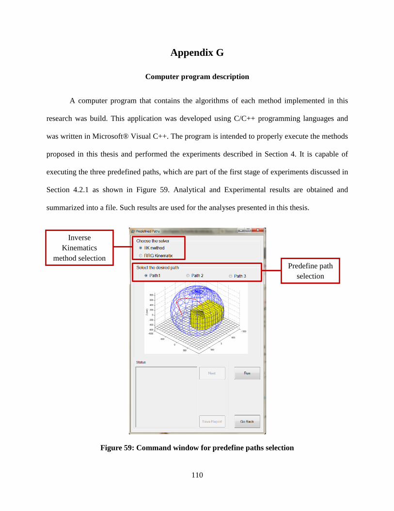
Appendix G
Computer program description
A computer program that contains the algorithms of each method implemented in this
research was build. This application was developed using C/C++ programming languages and
was written in Microsoft® Visual C++. The program is intended to properly execute the methods
proposed in this thesis and performed the experiments described in Section 4. It is capable of
executing the three predefined paths, which are part of the first stage of experiments discussed in
Section 4.2.1 as shown in Figure 59. Analytical and Experimental results are obtained and
summarized into a file. Such results are used for the analyses presented in this thesis.
Figure 59: Command window for predefine paths selection
Inverse Kinematics
method selection Predefine path
selection
110

The second stage of experiments consists of planning collision-free paths for ten different
scenarios. The program provides a friendly interface which allows the user to accurately model
the ten scenarios and to perform the pick-and-place operations using the obstacle avoidance
techniques described in Section 3.6. The program detects if the manipulator or the simulator are
connected and sends the proper commands to move the real or the virtual manipulator. When the
path planning algorithm is performed, the user provides the desired initial and final positions.
Two features were added to specify the location of the initial and final positions: numerical and
graphical interfaces. The location and dimensions of the obstacles must also be given by the user.
The dimensions of each obstacle are specified numerically and the location graphically, similar
to how the initial and final positions are given. The command window, designed to provide the
location of the initial and final points and the dimensions of the obstacles numerically, is shown
in Figure 60. The desired orientation of the end-effector can also be selected in this window.
Alternatively the point positions can be given using the graphical interface presented in Figure
61. As discussed in Section 5.2, the graphical interface can be enhanced by implementing a real
time visual sensor capable of capturing the location and dimensions of obstacles reducing human
interaction. This graphical interface represents the surrounding three dimensional space of the
manipulator and it is characterized by two two-dimensional maps (xy-view and xz-view). The
origin of the maps corresponds to the global Cartesian coordinate system of the manipulator
shown in Figure 8. The red line represents the borders of the wheeled mobile robot and the blue
line the workspace boundary of the manipulator. Each obstacle is also modeled and its
boundaries are characterized using gray lines. The red and blue crosses represent the initial and
final positions respectively.
111

Figure 60: Point positions selection and obstacle dimensions specifications
Figure 61: Graphical selection for point positions and obstacle locations
Numerical specifications for initial and final positions
Numerical specifications for obstacle
dimensions and patterns
End-effector orientation
specifications
Initial point position
Final point position
Rectangular obstacles
112
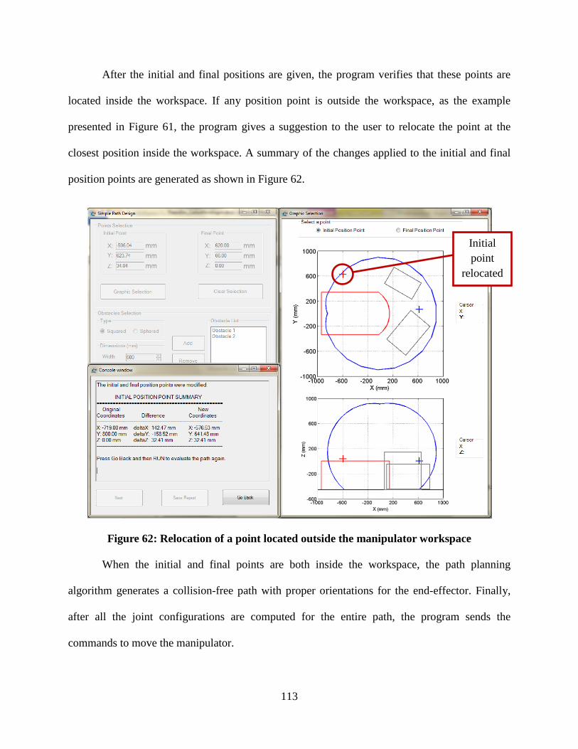
After the initial and final positions are given, the program verifies that these points are
located inside the workspace. If any position point is outside the workspace, as the example
presented in Figure 61, the program gives a suggestion to the user to relocate the point at the
closest position inside the workspace. A summary of the changes applied to the initial and final
position points are generated as shown in Figure 62.
Figure 62: Relocation of a point located outside the manipulator workspace
When the initial and final points are both inside the workspace, the path planning
algorithm generates a collision-free path with proper orientations for the end-effector. Finally,
after all the joint configurations are computed for the entire path, the program sends the
commands to move the manipulator.
Initial point
relocated
113

Appendix H
Simulation results for the remaining paths planned for 10 scenarios
This appendix presents the graphs of the joint angles and the normalized joint effort index
(Figures 64 to 81) obtained for nine of the ten scenarios presented in Section 4.2.2. The
remaining nine scenarios are shown in Figure 63.
(a)
(b)
(c)
(d)
114
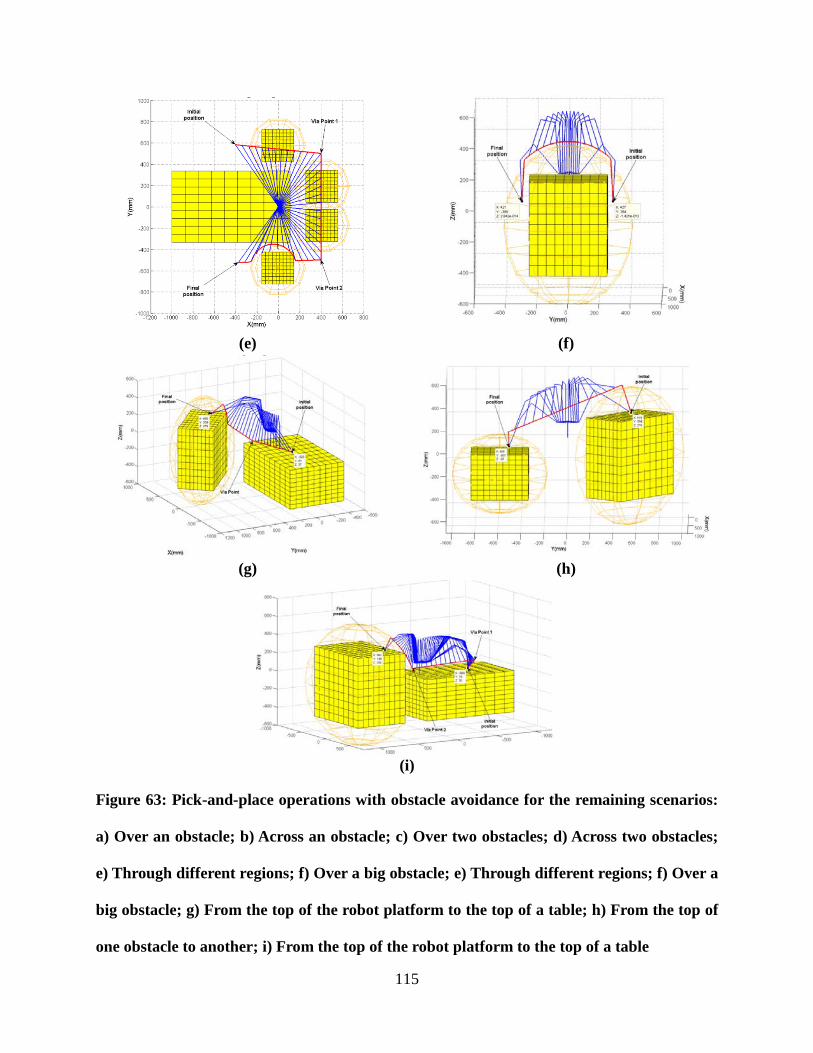
(e)
(f)
(g)
(h)
(i)
Figure 63: Pick-and-place operations with obstacle avoidance for the remaining scenarios:
a) Over an obstacle; b) Across an obstacle; c) Over two obstacles; d) Across two obstacles;
e) Through different regions; f) Over a big obstacle; e) Through different regions; f) Over a
big obstacle; g) From the top of the robot platform to the top of a table; h) From the top of
one obstacle to another; i) From the top of the robot platform to the top of a table
115

Figure 64: The 6-DOF Manipulator joint angles of the path shown in Figure 63a
Figure 65: Joint effort index of the path shown in Figure 63a
116

Figure 66: The 6-DOF Manipulator joint angles of the path shown in Figure 63b
Figure 67: Joint effort index of the path shown in Figure 63b
117

Figure 68: The 6-DOF Manipulator joint angles of the path shown in Figure 63c
Figure 69: Joint effort index of the path shown in Figure 63c
118

Figure 70: The 6-DOF Manipulator joint angles of the path shown in Figure 63d
Figure 71: Joint effort index of the path shown in Figure 63d
119

Figure 72: The 6-DOF Manipulator joint angles of the path shown in Figure 63e
Figure 73: Joint effort index of the path shown in Figure 63e
120

Figure 74: The 6-DOF Manipulator joint angles of the path shown in Figure 63f
Figure 75: Joint effort index of the path shown in Figure 63f
121

Figure 76: The 6-DOF Manipulator joint angles of the path shown in Figure 63g
Figure 77: Joint effort index of the path shown in Figure 63g
122

Figure 78: The 6-DOF Manipulator joint angles of the path shown in Figure 63h
Figure 79: Joint effort index of the path shown in Figure 63h
123

Figure 80: The 6-DOF Manipulator joint angles of the path shown in Figure 63i
Figure 81: Joint effort index of the path shown in Figure 63i
124

Appendix I
Experimental results for the remaining paths planned for 10 scenarios
This appendix presents the graphs of the joint angle error and the positioning error of the
end-effector (Figures 84 to 110) obtained when comparing the theoretical and experimental
results for nine of the ten paths introduced in Section 4.2.2. The plots for the joint velocities of
the 6-DOF manipulator for each path (Figures 84 to 110) are also presented. The remaining nine
scenarios are shown in Figure 82. Also, series of pictures are shown in Figure 83 to illustrate
some of the path planning experiments performed with the real manipulator.
(a)
(b)
(c)
(d)
125

(e)
(f)
(g)
(h)
(i)
Figure 82: Pick-and-place operations with obstacle avoidance for the remaining scenarios:
a) Over an obstacle; b) Across an obstacle; c) Over two obstacles; d) Across two obstacles;
e) Through different regions; f) Over a big obstacle; e) Through different regions; f) Over a
big obstacle; g) From the top of the robot platform to the top of a table; h) From the top of
one obstacle to another; i) From the top of the robot platform to the top of a table
126

a)
b)
c)
d)
Figure 83: Series of pictures for pick-and-place operations: a) Path No. 1 (Figure 82a);
b) Path No. 2 (Figure 82b); c) Path No. 3 (Figure 82c); d) Path No. 9 (Figure 82i)
127

Figure 84: Analytical versus experimental joint error for path shown in Figure 82a
Figure 85: Positioning error between analytical and experimental results for the end-
effector for the path shown in Figure 82a
Figure 86: Experimental joint velocity of the path shown in Figure 82a
128

Figure 87: Analytical versus experimental joint error for path shown in Figure 82b
Figure 88: Positioning error between analytical and experimental results for the end-
effector for the path shown in Figure 82b
Figure 89: Experimental joint velocity of the path shown in Figure 82b
129

Figure 90: Analytical versus experimental joint error for path shown in Figure 82c
Figure 91: Positioning error between analytical and experimental results for the end-
effector for the path shown in Figure 82c
Figure 92: Experimental joint velocity of the path shown in Figure 82c
130

Figure 93: Analytical versus experimental joint error for path shown in Figure 82d
Figure 94: Positioning error between analytical and experimental results for the end-
effector for the path shown in Figure 82d
Figure 95: Experimental joint velocity of the path shown in Figure 82d
131
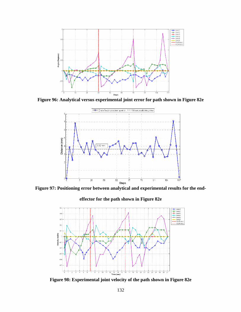
Figure 96: Analytical versus experimental joint error for path shown in Figure 82e
Figure 97: Positioning error between analytical and experimental results for the end-
effector for the path shown in Figure 82e
Figure 98: Experimental joint velocity of the path shown in Figure 82e
132

Figure 99: Analytical versus experimental joint error for path shown in Figure 82f
Figure 100: Positioning error between analytical and experimental results for the end-
effector for the path shown in Figure 82f
Figure 101: Experimental joint velocity of the path shown in Figure 82f
133

Figure 102: Analytical versus experimental joint error for path shown in Figure 82g
Figure 103: Positioning error between analytical and experimental results for the end-
effector for the path shown in Figure 82g
Figure 104: Experimental joint velocity of the path shown in Figure 82g
134

Figure 105: Analytical versus experimental joint error for path shown in Figure 82h
Figure 106: Positioning error between analytical and experimental results for the end-
effector for the path shown in Figure 82h
Figure 107: Experimental joint velocity of the path shown in Figure 82h
135
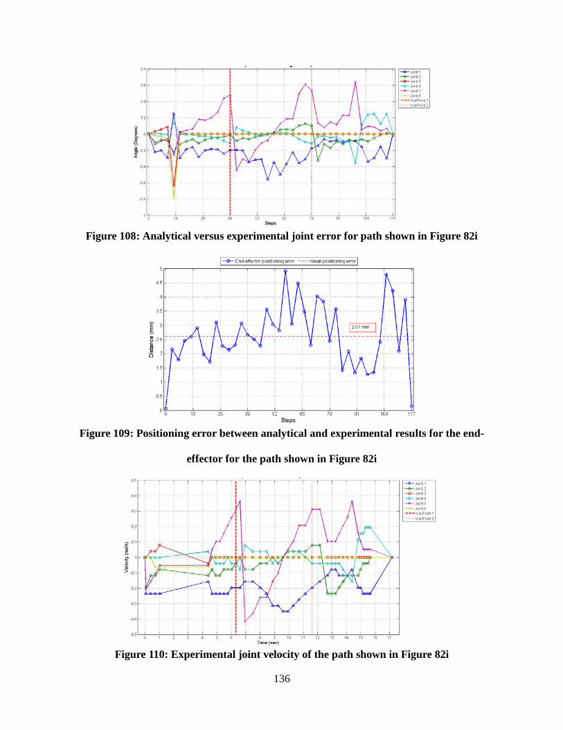
Figure 108: Analytical versus experimental joint error for path shown in Figure 82i
Figure 109: Positioning error between analytical and experimental results for the end-
effector for the path shown in Figure 82i
Figure 110: Experimental joint velocity of the path shown in Figure 82i
136