Dynamically Estimating the Distributional Impacts of U.S ...
40
Electronic copy available at: http://ssrn.com/abstract=2515617 Dynamically Estimating the Distributional Impacts of U.S. Climate Policy with NEMS: A Case Study of the Climate Protection Act of 2013 Danny Cullenward, 1,2,4* Jordan Wilkerson, 1,3,4 Michael Wara, 1,2 and John P. Weyant 1,3 1 Stanford Energy Policy Laboratory, Stanford University, CA USA 2 Stanford Law School, CA USA 3 Department of Management Science & Engineering, Stanford University, CA USA 4 Now at the Berkeley Energy and Climate Institute, University of California, Berkeley, CA USA * Corresponding author Address: 452 Sutardja Dai Hall, Berkeley, CA 94720 USA Email: [email protected] Phone: +1-510-664-7133 Abstract We present a new method that enables users of the federal government’s flagship energy policy model (NEMS) to dynamically estimate the direct cost impacts of climate policy across U.S. household incomes and census regions. Our approach combines NEMS output with detailed household expenditure data from the Consumer Expenditure Survey, improving on static methods that assess policy impacts by assuming household energy demand remains unchanged under emissions pricing scenarios. To illustrate our method, we evaluate a recent carbon fee-and- dividend proposal introduced in the U.S. Senate, the Climate Protection Act of 2013 (S. 332). Our analysis indicates this bill, if enacted, would have cut CO 2 emissions from energy by 17% below 2005 levels by 2020 at a gross cost of less than 0.5% of GDP, while simultaneously reducing direct energy expenditures for typical households making less than $120,000 per year and average households in all regions of the United States.
Transcript of Dynamically Estimating the Distributional Impacts of U.S ...

Electronic copy available at: http://ssrn.com/abstract=2515617
Dynamically Estimating the Distributional Impacts of U.S. Climate Policy with NEMS: A Case Study of the Climate Protection Act of 2013
Danny Cullenward,1,2,4* Jordan Wilkerson,1,3,4 Michael Wara,1,2 and John P. Weyant1,3
1 Stanford Energy Policy Laboratory, Stanford University, CA USA 2 Stanford Law School, CA USA 3 Department of Management Science & Engineering, Stanford University, CA USA 4 Now at the Berkeley Energy and Climate Institute, University of California,
Berkeley, CA USA
* Corresponding author Address: 452 Sutardja Dai Hall, Berkeley, CA 94720 USA Email: [email protected] Phone: +1-510-664-7133
Abstract
We present a new method that enables users of the federal government’s flagship energy
policy model (NEMS) to dynamically estimate the direct cost impacts of climate policy across
U.S. household incomes and census regions. Our approach combines NEMS output with detailed
household expenditure data from the Consumer Expenditure Survey, improving on static
methods that assess policy impacts by assuming household energy demand remains unchanged
under emissions pricing scenarios. To illustrate our method, we evaluate a recent carbon fee-and-
dividend proposal introduced in the U.S. Senate, the Climate Protection Act of 2013 (S. 332).
Our analysis indicates this bill, if enacted, would have cut CO2 emissions from energy by 17%
below 2005 levels by 2020 at a gross cost of less than 0.5% of GDP, while simultaneously
reducing direct energy expenditures for typical households making less than $120,000 per year
and average households in all regions of the United States.

Electronic copy available at: http://ssrn.com/abstract=2515617
Dynamically Estimating the Distributional Impacts of U.S. Climate Policy with NEMS Page 2 of 40
1. Introduction
Analyzing the costs and benefits of U.S. climate policy raises complex methodological
problems. Many tools are available to estimate the national economic, environmental, and fiscal
impacts of proposed policies, yet none of the standard national energy models is capable of
projecting the costs of climate policy across household income levels. With increasing interest in
the cost of climate policy for low-income households, including the development of policy
proposals designed to mitigate these impacts, policymakers need new analytical tools.
Here, we describe a new method by which users of a prominent energy model can better
evaluate the distributional impacts of prospective climate policies. Our approach focuses on the
National Energy Modeling System (NEMS), the federal government’s flagship energy-economic
model. NEMS is widely used by academics, policymakers, and consultants to assess national
energy and climate policies. For example, the U.S. Energy Information Administration uses
NEMS to generate its Annual Energy Outlook (AEO), a report that projects energy consumption
and related trends over a 20-25 year horizon (EIA, 2012a). EIA also uses NEMS to evaluate
prospective energy and climate policies (EIA, 2010a, 2010b, 2009a, 2008a, 2008b, e.g., 1998).
We develop a method that couples NEMS output with data from the Consumer
Expenditure Survey (CEX), which reports household energy expenditures across income levels
and geography (BLS, 2013). By linking NEMS output and CEX data, we are able to dynamically
estimate net changes in household energy expenditures, also known as “direct” policy costs (see
Section 2.3.3 for a discussion of direct and indirect costs). This approach offers important
advantages over existing methods for estimating direct costs, which generally assume that
households have a static demand for energy, despite the introduction of a price on carbon dioxide
(CO2) emissions. For example, Metcalf (1999) calculates the incidence of a carbon tax across
household income levels using CEX data. Metcalf estimates the effect of a carbon tax on the

Electronic copy available at: http://ssrn.com/abstract=2515617
Dynamically Estimating the Distributional Impacts of U.S. Climate Policy with NEMS Page 3 of 40
price of goods and services in the national economy by propagating it through an input-output
matrix of inter-industry transactions. The impact on households depends on these price changes
and the consumption patterns across household incomes, which are described in the CEX data.
Notably, his method assumes both that the structure of the economy and the composition of
household expenditures remains unchanged, a feature that many other papers in the field share
(e.g., Hassett et al., 2009; Mathur and Morris, 2014; Metcalf, 2009). Our approach is most
closely related to Blonz et al. (2011), who estimate the distribution of climate policy costs across
household income levels by combining CEX data on consumption patterns with projections of
future consumption derived from energy-economic models. Specifically, Blonz et al. use EIA’s
reference forecast (based on NEMS) to project changes in consumption outside the electricity
sector and an RFF model (Haiku) to project changes in electricity consumption. As a result, one
of the model drivers is static (EIA’s reference forecast for non-electricity) and another is
dynamic (RFF’s policy scenario for electricity). Yet CEX data show that electricity represents
only a quarter of average American household energy expenditures, suggesting the need for
dynamic analysis of additional expenditures.
Our approach offers a modest but important improvement over past work in two respects.
First, we integrate dynamic modeling results for all energy-related household consumption over
multiple years. This allows us to include expected changes in household energy-related
consumption in our estimate of direct policy costs. Second, we use the federal government’s own
energy model, NEMS. Both features enable comparison of our results with standard government
forecasts and official government policy analysis. Our dynamic estimates of direct costs can be
combined with other researchers’ estimates of indirect costs (e.g., Mathur and Morris, 2014) to
assess the full impact on consumer welfare, or compared against relevant portions of the results
Dynamically Estimating the Distributional Impacts of U.S. Climate Policy with NEMS Page 4 of 40
from stand-alone general equilibrium models (Goulder and Hafstead, 2013; Williams et al.,
2014) that are used to assess the distributional impacts of prospective climate policies.
To illustrate our method’s applications, we analyze a recent carbon fee-and-dividend
policy proposed in the U.S. Senate. A distributional analysis is particularly relevant for policies
of this nature because they are designed to protect the lowest-income households from increased
energy costs through lump-sum tax revenue rebates. The Climate Protection Act of 2013
(S. 332), introduced by Senators Barbara Boxer (D-CA) and Bernie Sanders (I-VT), would have
imposed a carbon pollution fee on CO2 emissions from fossil fuels. The fee would have started in
2014 at $20 per metric ton of CO2 and rising at 5.6% per year in nominal terms through 2023
(Boxer and Sanders, 2013). Under the bill, 60% of revenue collected from the carbon fee would
be returned to legal residents of the United States in the form of monthly dividends. The bill also
included a number of energy policy programs, including those designed to protect trade-exposed
industries ($75 billion), provide financial assistance to weatherize low-income homes ($50
billion), job training and transition assistance ($10 billion), energy R&D ($20 billion), and
energy finance ($50 billion). Collectively, these expenditures would have accounted for about
16% of total carbon revenues that would have been collected over the first ten years of the
policy. The balance of carbon revenues (about 24%) would have been used to reduce the federal
government’s deficit, per the Senate PAYGO rules (CBO, 2009).1
1 Technically, the bill first apportions 60% of revenues for rebates, then allocates specific amounts to policy
programs, and finally directs the remaining revenue to deficit reduction. Thus, the deficit reduction depends on the total revenue raised. We show in Section 3.3 that just over 24% of total revenues would be available for deficit reduction, suggesting compliance with U.S. Senate pay-as-you-go (PAYGO) rules is feasible. According to PAYGO rules, legislation that imposes new taxes or fees on the economy must discount its expected revenues by 25% to account for the indirect reductions in federal income and payroll taxes (CBO, 2009).

Dynamically Estimating the Distributional Impacts of U.S. Climate Policy with NEMS Page 5 of 40
Our paper is organized as follows. Section 2 describes the energy economic model
(NEMS) and external CEX household data used in this study, along with our method for
integrating these analytical tools. Next, we apply our method to the Climate Protection Act of
2013. Section 3 describes the environmental, economic, and fiscal results of our modeling work,
including a detailed treatment of how the Act would impact household-level expenditures on
energy across income levels and geographic regions. We discuss the results and review key
assumptions in Section 4. Finally, Section 5 summarizes our findings and suggests directions for
future work.
2. Model, methods, and approach
Assessing the impacts of a federal carbon price on both the U.S. economy and on individual
households requires more than a single modeling tool. We use NEMS to estimate changes at the
national level, projecting the emission reductions, macroeconomic impacts, and fiscal
consequences of the carbon fee. These results are then combined with the Consumer Expenditure
Survey (CEX), which identifies how much different households spend on energy goods and
services. We estimate future energy-related expenditure by coupling NEMS projections of
energy prices and consumption to their corresponding metrics in the CEX, allowing us to
consistently estimate the effect of changing energy markets on household energy expenditures.
The following sub-sections describe NEMS, the CEX data, and our method for combining these
tools to assess the Climate Protection Act.
2.1 Energy-economic model: NEMS
NEMS is arguably the most influential U.S. energy model. EIA uses NEMS to generate
the federal government’s annual long-term forecast of national energy consumption and to

Dynamically Estimating the Distributional Impacts of U.S. Climate Policy with NEMS Page 6 of 40
evaluate prospective federal energy policies (EIA, 2009b). NEMS is considered such an
important tool that other models are calibrated to its forecasts, in both government and academic
practice. Consequently, it has a significant influence over expert opinions of plausible energy
futures. EIA uses NEMS to evaluate the impacts of proposed energy and climate policies, often
at the request of Congress. Some examples include the analysis of the Kyoto Protocol
greenhouse gas (GHG) emissions limits (EIA, 1998), the Lieberman‒Warner Climate Security
Act (EIA, 2008a), the Low Carbon Economy Act (EIA, 2008b), the Waxman‒Markey American
Clean Energy and Security (ACES) Act (EIA, 2009a), the American Power Act (EIA, 2010a),
and Carbon Limits and Energy for America’s Renewal (CLEAR) Act (EIA, 2010b).
Because of the model’s prevalence, many other government, academic, and private sector
studies use NEMS to assess prospective energy and climate policies. For example, the U.S.
Department of Energy's Office of Energy Efficiency and Renewable Energy (EERE)
commissioned a group of national laboratory scientists to conduct a follow-up report to the EIA’s
study of the costs of complying with the Kyoto Protocol (Brown et al., 2001). Other examples
include a prospective analysis of the impact of a federal renewable portfolio standard on U.S.
energy markets (Kydes, 2007), the impacts from the 1990 Clean Air Act Amendments (Luong et
al., 1998), an analysis of polices to reduce oil consumption and GHG emissions from the U.S.
transportation sector (Morrow et al., 2010), the impact of climate and energy policies on the U.S.
forest products industry (Brown and Baek, 2010), the effects of climate policy on freshwater
withdrawals for thermoelectric power generation (Chandel et al., 2011), and energy efficiency
potential in the residential and commercial building sectors (Wilkerson et al., 2013). Consulting
groups, such as McKinsey & Company (Choi Granade et al., 2009; Creyts et al., 2007) and the

Dynamically Estimating the Distributional Impacts of U.S. Climate Policy with NEMS Page 7 of 40
Rhodium Group (Houser and Mohan, 2014) also use NEMS to analyze trends and policies that
affect the broader U.S. energy-economy.
The model’s popularity is due in part to its massively detailed representation of the U.S.
energy-economic structure, which allows for a plausible simulation of energy supplies and
demand within different sectors. However, several aspects of the model create difficulties when
the model is used to evaluate prospective carbon tax policies. While NEMS has some ability to
estimate the geographic impacts of climate policy, these calculations are made at a high level,
with results aggregated at the level of nine U.S. Census Divisions. Furthermore, understanding
how policy costs fall across income levels is a key step to designing the appropriate level of
compensation for policies that propose to rebate a portion of the total revenue to consumers. Yet
NEMS does not analyze the impacts of prospective policies across different household income
levels, nor does it track any household-level or individual consumer impacts. The model
provides only aggregated output on income- and tax-related forecasts for consumers and firms.
As a result, developing an estimate of the distributional impact of climate policies requires
combining NEMS forecasts with external data sources.
2.2 Household energy expenditures
To assess the impact to households across income groups and location, we couple NEMS
output with the U. S. Bureau of Labor Statistics’ 2011 Consumer Expenditure Survey (CEX),
which provides cross-sectional data on household expenditures (BLS, 2013). CEX is perhaps the
most comprehensive survey on consumer expenditures, providing cross-sectional data on all
household expenditures, income, and other characteristics. The annual report provides detailed
expense summaries on various activities including type of foods, rent and mortgage, utilities,
furnishings, apparel, healthcare, transportation, entertainment, and others. The survey data are

Dynamically Estimating the Distributional Impacts of U.S. Climate Policy with NEMS Page 8 of 40
used by policymakers, businesses and academic researchers, and by other Federal agencies—
including to regularly revise the Consumer Price Index (CPI).
2.3 Approach
Our methodology involves three steps. First, we use NEMS to forecast the impact of carbon
prices on energy-related emissions, gross domestic product (GDP), energy demand, and energy
prices. Second, we connect relevant NEMS output on energy demand and prices to their
corresponding expenditure categories in the CEX. Specifically, we scale the energy expenditure
patterns reported in the CEX data by the expected changes in residential energy prices and
energy consumption due to climate policy, as projected by NEMS. This method allows us to
assess policy impacts across household income levels and geography. Third, we complete our
analysis of the impacts to household expenditures by rebating a portion of the total revenues to
households on a per capita basis. Each step is described in more detail below.
2.3.1 Modifying and running NEMS
Applying a carbon fee within the NEMS framework is relatively straightforward. Carbon
prices are set in the emissions policy data file epmdata.txt, which is read by the model when the
code is initiated. This input requires an explicit annual carbon price series, expressed in
1987$/kgC for each year. For detailed description of this file and the emissions policy
submodule, see the NEMS Integrating Module documentation (EIA, 2010c). Consistent with the
Climate Protection Act, we modeled a nominal $20/tCO2 price that begins in 2014 and escalates
at 5.6% (nominal) each year for ten years.
In addition to specifying carbon price levels, NEMS users must tell the model how to account
for the revenue collected by the climate policy. The model has several default options for how its
macroeconomic calculations treat the use of carbon fee revenues. These options are set with the
Dynamically Estimating the Distributional Impacts of U.S. Climate Policy with NEMS Page 9 of 40
mactax flag in the scedes (scenario description) file. The flag is subsequently used by the
mcevcode.txt text file, which serves as an interface between the core model code and the
Macroeconomic Activity Module (EIA, 2013a). The value of mactax can be set from 0 to 5. A
value of 0 turns carbon pricing off, while settings 1 through 5 turn carbon pricing on with binary
control over how revenues are recycled through the economy. Tax modes 1 and 2 return
revenues to consumers and businesses, respectively, in a revenue-neutral manner; tax mode 3
applies all revenues to federal government deficit reduction; tax modes 4 and 5 return revenues
to consumers and businesses, respectively, in a deficit-neutral manner.
Revenue use under the Climate Protection Act includes consumer rebates, deficit
reduction, and policy expenditures; however, none of the default options in NEMS permits a
mixture of these approaches, nor does any account for the re-spending effects of government
policies. We found that the choice of default revenue options does not materially affect GDP,
greenhouse gas emissions, or residential energy prices.2 This result is surprising, but may reflect
the relative simplicity of the NEMS macroeconomic module’s treatment of tax policy, a common
model limitation raised by (Fawcett et al., 2014). Many studies have suggested that the choice of
mechanism for revenue recycling—such as lump-sum transfers, income tax reductions, or
corporate tax reductions—should have important macroeconomic and efficiency implications
and can lead to more efficient outcomes if the revenues are used to reduce the level of ordinary
distortionary taxes (Goulder and Hafstead, 2013; Goulder, 2013; Williams et al., 2014).
Nonetheless, having confirmed that the choice of revenue recycling modes did not affect
our results, we set mactax to 4, which recycles all revenue back to households for the purposes of 2 The NEMS interface with the Macroeconomic Activity Module (MAM) is the mcevcode.txt file, which is used to
pass values and settings to the MAM. With some additional coding in that file, these default options can be combined. However, the different revenue options do not materially affect GDP or net greenhouse gas emissions. This result is illustrated in Appendix A.7 in Wilkerson (2014).

Dynamically Estimating the Distributional Impacts of U.S. Climate Policy with NEMS Page 10 of 40
the model’s internal macroeconomic analysis. This setting is also what EIA uses for their carbon
price sensitivity studies, as described in Appendix D of the AEO2013 (EIA, 2013b).
Finally, we note that our analysis is based on an independent version of the 2013 release
of NEMS. To ensure the model and its third-party software components were properly installed
and engaged, we confirmed that the local version of the model accurately reproduced the EIA’s
published baseline scenario projections. Thus, our local setup is a reliable means of assessing
what EIA’s official copy of NEMS would project for the same scenarios modeled here.
Nevertheless, our results independent and should not be confused with official government
policy analysis. Accordingly, outputs from this study are designated as coming from NEMS-
Stanford, an independent and unofficial copy of the government’s model.
2.3.2 Bridging NEMS forecasts with CEX data
The CEX includes approximately one hundred household expenditure line items, but only
five correspond to energy-related goods and services: natural gas, electricity, fuel oil and other
household fuels, gasoline and motor oil, and public and other transportation. In 2011, the average
American household spent $5,171 on energy-related activities, which was 10.4% of total average
household expenses. Expressed as a percentage of total energy expenditures, the average
household spent about 51% on gasoline, 28% on electricity, 10% on public and other transit
(including airline travel), 8% on natural gas, and the remaining 3% on fuel oils and other fuels.
As the CEX data show, however, energy expenditures vary significantly by household
income level, with households in higher income brackets spending more money—though a
smaller percentage of their overall income—on energy. Figure 1 illustrates energy expenditures
for the average American household and the five quintiles of income distribution in 2011.
Energy expenditures for average households of different income levels and in different

Dynamically Estimating the Distributional Impacts of U.S. Climate Policy with NEMS Page 11 of 40
geographic regions are reported in Table 1. The disparity in both total quantity and relative
expenditure shares on different energy types varies significantly across income quintiles. The
largest variation by income in quantity of energy expenditures occurs for purchases of gasoline,
while the largest percentage variation by income occurs for “other transportation,” which
includes air travel. In turn, this variation illustrates the importance of assessing carbon policy
impacts across income distributions.
Figure 1: Average household energy expenditures by income quintile in 2011

Dynamically Estimating the Distributional Impacts of U.S. Climate Policy with NEMS Page 12 of 40
Table 1: U.S. household energy expenditures by income and geographic region in 2011
Total
thou
s.% of
totalpp
h¹Income²
$/HH
$/HH
% of
Total$/HH
% of
energy
Inde
x³$/HH
% of
energy
Inde
x³$/HH
% of
energy
Inde
x³$/HH
% of
energy
Inde
x³$/HH
% of
energy
Inde
x³
Average Ho
useh
old
122,287
100%
2.5
$61,673
$49,705
$5,171
10.4%
$420
8.1%
1.00
$1,423
27.5%
1.00
$157
3.0%
1.00
$2,655
51.3%
1.00
$516
10.0%
1.00
By Income Quintile
s24,435
20%
1.7
$10,074
$22,001
$2,722
12.4%
$243
8.9%
0.58
$985
36.2%
0.69
$85
3.1%
0.54
$1,227
45.1%
0.46
$182
6.7%
0.35
24,429
20%
2.2
$27,230
$32,092
$3,876
12.1%
$338
8.7%
0.80
$1,234
31.8%
0.87
$119
3.1%
0.76
$1,981
51.1%
0.75
$204
5.3%
0.40
24,473
20%
2.6
$45,563
$42,403
$5,016
11.8%
$386
7.7%
0.92
$1,429
28.5%
1.00
$140
2.8%
0.89
$2,694
53.7%
1.01
$367
7.3%
0.71
24,520
20%
2.8
$72,169
$57,460
$6,015
10.5%
$472
7.8%
1.12
$1,603
26.7%
1.13
$170
2.8%
1.08
$3,295
54.8%
1.24
$475
7.9%
0.92
24,430
20%
3.2$153,326
$94,551
$8,217
8.7%
$659
8.0%
1.57
$1,863
22.7%
1.31
$270
3.3%
1.72
$4,073
49.6%
1.53
$1,352
16.5%
2.62
By Region
22,538
18.4%
2.4
$69,334
$54,547
$5,661
10.4%
$596
10.5%
1.42
$1,338
23.6%
0.94
$487
8.6%
3.10
$2,510
44.3%
0.95
$730
12.9%
1.41
27,107
22.2%
2.4
$59,394
$47,192
$5,031
10.7%
$600
11.9%
1.43
$1,225
24.3%
0.86
$121
2.4%
0.77
$2,632
52.3%
0.99
$453
9.0%
0.88
44,901
36.7%
2.5
$57,205
$45,699
$5,204
11.4%
$243
4.7%
0.58
$1,763
33.9%
1.24
$70
1.3%
0.45
$2,794
53.7%
1.05
$334
6.4%
0.65
27,741
22.7%
2.6
$64,909
$54,745
$4,853
8.9%
$387
8.0%
0.92
$1,135
23.4%
0.80
$64
1.3%
0.41
$2,569
52.9%
0.97
$698
14.4%
1.35
By Hou
seho
ld Income
4,978
4.1%
1.7
-‐$995
$22,960
$2,578
11.2%
$241
9.3%
0.57
$909
35.3%
0.64
$49
1.9%
0.31
$1,148
44.5%
0.43
$231
9.0%
0.45
5,449
4.5%
1.7
$8,155
$20,884
$2,470
11.8%
$201
8.1%
0.48
$900
36.4%
0.63
$100
4.0%
0.64
$1,112
45.0%
0.42
$157
6.4%
0.30
8,170
6.7%
1.6
$12,803
$19,959
$2,667
13.4%
$229
8.6%
0.55
$1,006
37.7%
0.71
$87
3.3%
0.55
$1,172
43.9%
0.44
$173
6.5%
0.34
7,745
6.3%
2.0
$17,955
$24,806
$3,220
13.0%
$316
9.8%
0.75
$1,127
35.0%
0.79
$113
3.5%
0.72
$1,487
46.2%
0.56
$177
5.5%
0.34
14,460
11.8%
2.2
$25,136
$30,398
$3,830
12.6%
$324
8.5%
0.77
$1,215
31.7%
0.85
$132
3.4%
0.84
$1,971
51.5%
0.74
$188
4.9%
0.36
13,328
10.9%
2.4
$34,750
$36,769
$4,299
11.7%
$371
8.6%
0.88
$1,302
30.3%
0.91
$97
2.3%
0.62
$2,247
52.3%
0.85
$282
6.6%
0.55
11,347
9.3%
2.6
$44,196
$40,306
$4,977
12.3%
$380
7.6%
0.90
$1,433
28.8%
1.01
$142
2.9%
0.90
$2,679
53.8%
1.01
$343
6.9%
0.66
17,376
14.2%
2.7
$58,070
$50,034
$5,471
10.9%
$427
7.8%
1.02
$1,516
27.7%
1.07
$158
2.9%
1.01
$2,961
54.1%
1.12
$409
7.5%
0.79
7,385
6.0%
2.8
$72,895
$57,977
$6,003
10.4%
$462
7.7%
1.10
$1,600
26.7%
1.12
$169
2.8%
1.08
$3,345
55.7%
1.26
$427
7.1%
0.83
10,456
8.6%
3.0
$86,417
$65,390
$6,643
10.2%
$522
7.9%
1.24
$1,662
25.0%
1.17
$187
2.8%
1.19
$3,612
54.4%
1.36
$660
9.9%
1.28
7,045
5.8%
3.2$105,125
$76,496
$7,298
9.5%
$603
8.3%
1.44
$1,710
23.4%
1.20
$228
3.1%
1.45
$3,921
53.7%
1.48
$836
11.5%
1.62
6,107
5.0%
3.1$127,734
$87,239
$8,048
9.2%
$598
7.4%
1.42
$1,760
21.9%
1.24
$267
3.3%
1.70
$4,150
51.6%
1.56
$1,273
15.8%
2.47
8,440
6.9%
3.2$232,086
$123,056
$9,551
7.8%
$779
8.2%
1.85
$2,147
22.5%
1.51
$331
3.5%
2.11
$4,267
44.7%
1.61
$2,027
21.2%
3.93
Notes:¹P
eople pe
r hou
seho
ld²After taxes
³Inde
xed to Avg. Con
sumer Unit
Gasolin
e & Motor Oil
Other Transpo
rtation
Energy
Energy Expen
diture by Fuel Type: $/HH, % of e
nergy expe
nditu
res, inde
xed to average co
nsum
erExpe
nditu
reNatural Gas
Electricity
Fuel oil & Other Fue
lHo
useh
olds
Less th
an $5k (H
H1)
Market Segmen
t
Lowest 20 % (Q
1)
Highest 20 % (Q
5)Fourth 20 % (Q
4)Third
20 % (Q
3)Second
20 % (Q
2)
West (W)
Avg. Con
sumer Unit
South (S)
Midwest (MW)
Northeast (N
E)
$150k and more (HH1
3)$120k to <$150k (HH1
2)$100k to <$120k (HH1
1)$80k to
<$100k (HH1
0)$70k to
<$80k (H
H9)
$10k to
<$15k (H
H3)
$5k to <$10k (H
H2)
$50k to
<$70k (H
H8)
$40k to
<$50k (H
H7)
$30k to
<$40k (H
H6)
$20k to
<$30k (H
H5)
$15k to
<$20k (H
H4)

Dynamically Estimating the Distributional Impacts of U.S. Climate Policy with NEMS Page 13 of 40
In order to link CEX and NEMS, the energy-related expenditures in the CEX data are
matched to their corresponding outputs from NEMS, as shown in Table 2. Note that while
NEMS output includes detailed output that corresponds to most energy consumption data series
in CEX, we were unable to match a direct proxy for “public and other transportation”—a
category that includes significant air travel. As a result, we assumed percentage changes in
expenditures in this category would be comparable to those for gasoline. Indeed, the relative
price trends for gasoline and the mixture of gasoline, diesel, and jet fuel in the “public and other
transportation” category should be quite similar. It is nevertheless possible that the price
elasticity of demand differs across fuels or transportation services, in which case our assumption
would introduce bias.
Table 2: Correspondence between CEX and NEMS
CEX Series NEMS Output
Natural gas Residential natural gas prices and quantities
Electricity Residential electricity prices and quantities
Fuel oil and other fuels Consumption-weighted average of residential prices and quantities for propane, kerosene, and distillate fuel oil
Gasoline and motor oil Retail gasoline prices and population-weighted shares of national consumption of gasoline for light duty vehicles
Public and other transportation Retail gasoline prices and population-weighted shares of national consumption of gasoline for light duty vehicles.
Next, we use NEMS forecasts for residential energy expenditures to project trends based
on historic CEX household expenditures. Each scenario in NEMS produces a forecast of energy
prices (𝑃) and a total aggregate consumption (𝑄) for each major fuel types (𝑓). The product of
this price and quantity forecast in a given region (or the U.S. as a whole) is the total cost for each
fuel within the residential sector for a given year (𝑦). Equation 1 shows the difference in total

Dynamically Estimating the Distributional Impacts of U.S. Climate Policy with NEMS Page 14 of 40
expenditure between the Reference and a policy scenario represents the annual cost of the policy
for each fuel type (𝐶!!). These impacts correspond to what economists have called the “direct
component” of total impacts (Hassett et al., 2009; Mathur and Morris, 2014).
𝐶!! = (𝑃 ∙ 𝑄)!
!!"#$%&
− (𝑃 ∙ 𝑄)!!!"#"!"$%"
Eq. 1
Linking the CEX data is a matter of scaling the CEX 2011 household energy expenditure
data (𝐸!!"##) by the total aggregate expenditure from NEMS in the same year (See Equation 2).
This produces a per-household share of total residential energy expenditure.
𝐸!!"!!
𝑃 ∙ 𝑄 !!"## Eq. 2
The direct cost to household energy expenditures in a given year is therefore the sum of
the products of Equations 1 and 2 for all five fuel types (f).
Household Direct Cost! = 𝐸!!"## ∙𝑃 ∙ 𝑄 !
!
𝑃 ∙ 𝑄 !!"##
!
Eq. 3
This method works well when NEMS outputs are of equal or higher resolution as the
CEX survey data. Although each of its component modules uses a different resolution when
making internal calculations, NEMS generally reports most results at the national level and for
each of nine Census Divisions, whereas CEX reports published data for four Census Regions.
Thus, when linking the CEX Region data to NEMS, we first aggregate the nine Census Divisions
from NEMS into the appropriate Census Region (see Table 3).
Dynamically Estimating the Distributional Impacts of U.S. Climate Policy with NEMS Page 15 of 40
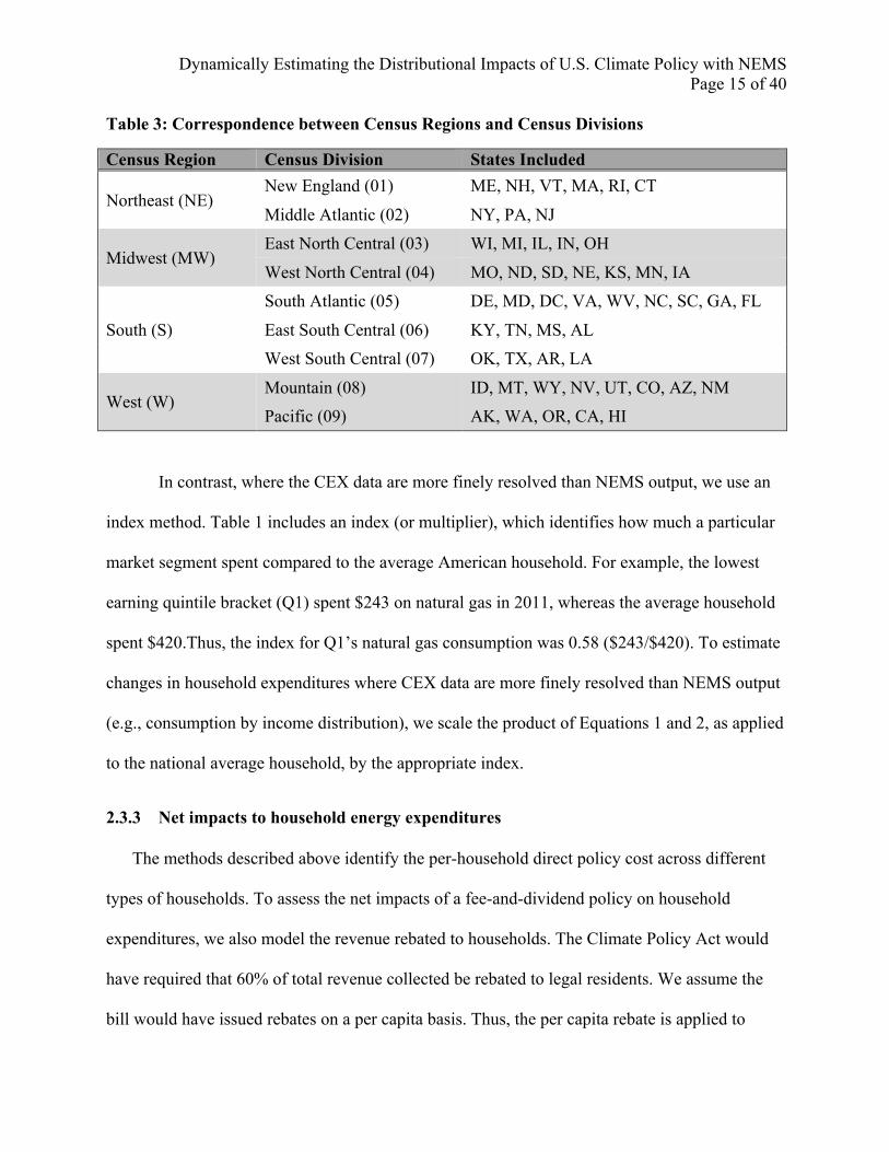
Table 3: Correspondence between Census Regions and Census Divisions
Census Region Census Division States Included
Northeast (NE) New England (01) ME, NH, VT, MA, RI, CT
Middle Atlantic (02) NY, PA, NJ
Midwest (MW) East North Central (03) WI, MI, IL, IN, OH
West North Central (04) MO, ND, SD, NE, KS, MN, IA
South (S)
South Atlantic (05) DE, MD, DC, VA, WV, NC, SC, GA, FL
East South Central (06) KY, TN, MS, AL West South Central (07) OK, TX, AR, LA
West (W) Mountain (08) ID, MT, WY, NV, UT, CO, AZ, NM Pacific (09) AK, WA, OR, CA, HI
In contrast, where the CEX data are more finely resolved than NEMS output, we use an
index method. Table 1 includes an index (or multiplier), which identifies how much a particular
market segment spent compared to the average American household. For example, the lowest
earning quintile bracket (Q1) spent $243 on natural gas in 2011, whereas the average household
spent $420.Thus, the index for Q1’s natural gas consumption was 0.58 ($243/$420). To estimate
changes in household expenditures where CEX data are more finely resolved than NEMS output
(e.g., consumption by income distribution), we scale the product of Equations 1 and 2, as applied
to the national average household, by the appropriate index.
2.3.3 Net impacts to household energy expenditures
The methods described above identify the per-household direct policy cost across different
types of households. To assess the net impacts of a fee-and-dividend policy on household
expenditures, we also model the revenue rebated to households. The Climate Policy Act would
have required that 60% of total revenue collected be rebated to legal residents. We assume the
bill would have issued rebates on a per capita basis. Thus, the per capita rebate is applied to

Dynamically Estimating the Distributional Impacts of U.S. Climate Policy with NEMS Page 16 of 40
households based on the average number of occupants (see Table 1). Accordingly, the net impact
to household energy expenditures is defined as the difference between the increase in direct
energy costs and the rebate under the fee-and-dividend policy. Notably, we report only direct
costs, which do not include impacts to employment, GDP, or any other macroeconomic changes.
Static estimates of indirect costs suggest that they could add an additional 50 to 100% above the
direct cost estimate for the different household income categories, though indirect costs are
significantly less regressive than are direct costs (Mathur and Morris, 2014: Table 1). In addition,
like other papers that project CEX data forward with model results, this study assumes that
income distribution patterns do not change during the forecast period.
3. Results
3.1 Avoided carbon dioxide emissions from fossil fuel use
Our analysis indicates that the carbon pollution fee implemented under the Climate
Protection Act would significantly reduce energy-related CO2 emissions across the U.S.
economy in the next decade. Over the first ten years of the program (2014-2023), the bill would
have avoided aggregate emissions by more than 4,200 MMt CO2, relative to the reference
scenario. Emission reductions occur rapidly during the first two years of implementation,
slowing to a more gradual decline in subsequent years. This reduction is in stark contrast to the
baseline scenario, in which energy-related CO2 emissions are expected to increase during the
next decade, following sharp declines in the period from 2008 to 2011 (see Figure 2).

Dynamically Estimating the Distributional Impacts of U.S. Climate Policy with NEMS Page 17 of 40
Figure 2: Estimated reductions in energy-related CO2 emissions
Due to the Climate Protection Act, U.S. CO2 emissions from energy in 2023 would have
been 575 MMtCO2 (10.5%) less than in the reference scenario. By pricing CO2 emissions, the
Climate Protection Act would have extended the reduction in emissions observed since 2007,
marking that year as the peak for national emissions of CO2 from energy use.
Under the Copenhagen Accord (UNFCCC, 2010), the U.S. has committed to reduce its
economy-wide GHG emissions to “in the range of 17% below” 2005 levels by 2020. Although
the Climate Protection Act does not mandate any specific reductions levels, NEMS-Stanford
projects that the carbon fee would have reduced energy-related CO2 emissions in 2020 by 8.5%
(464 MMtCO2) below reference scenario emissions. This is equivalent to 16.8% (1,009
MMtCO2) below 2005 energy-related CO2 emissions, putting the U.S. within reach of its pledge
under the Copenhagen Accord. Note that the U.S. commitment under the Copenhagen Accord
could be read to cover emissions of six greenhouse gases (CO2, methane, nitrous oxide,

Dynamically Estimating the Distributional Impacts of U.S. Climate Policy with NEMS Page 18 of 40
hydrofluorocarbons, perfluorocarbons, and sulfur hexafluoride), whereas NEMS projects only
energy-related CO2 emissions, a subset of emissions that accounts for approximately 79% of
gross and 91% of net GHG emissions in the United Sates (EIA, 2012b).
We also review how the emission reductions would have been achieved. Figure 3 shows
that almost all of the avoided emissions would come from changes in the electricity supply
sector—87% of total avoided emissions over the policy’s first decade. Changes in demand for
petroleum and natural gas outside of the electricity sector account for 6.5% and 6.2% of total
reductions, respectively, while changes in direct-use coal provides less than 1% of emission
reductions.
Figure 3: Avoided emissions by fuel type
Figure 4 provides additional detail, illustrating changes in the quantity of fuels used to
generate electricity under the Climate Protection Act. NEMS-Stanford projects an immediate
response to the policy in which generation switches away from coal-fired and toward natural gas-
fired power plants. In the first year of the policy, an 18% reduction in coal use is matched with
19% increase in natural gas use. These two resources represent 40% and 27% of total electricity

Dynamically Estimating the Distributional Impacts of U.S. Climate Policy with NEMS Page 19 of 40
generation (respectively) in 2013 (see Figure 5). Despite significant fuel-switching activities,
however, total electricity generation falls by only about 5%, compared to the reference scenario,
with most demand reduction occurring within the first few years. This result is consistent with
earlier studies that suggest that changes in end-use energy efficiency as projected by NEMS are
primarily driven by user inputs, not energy prices (Wilkerson et al., 2013). Thus, when NEMS-
Stanford includes a price for CO2 emissions, the model projects that the electricity sector
switches from coal to gas on the margin. Since many natural gas power plants currently have
spare capacity, the electricity sector can immediately re-dispatch production; in addition, the
model projects that some coal plants would retire in response to the carbon price.3
3 We note that coal power plant retirement occurs three years after the carbon price is introduced, which likely
reflects the model structure. Although NEMS calculates whether power plants will stay in operation or retire, uneconomic conditions must subsist for three years before the model allows retirement. While this assumption may be sensible for considering normal market reactions to commodity prices, it may not hold in the case of an explicit change in government policy.
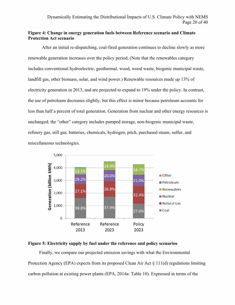
Dynamically Estimating the Distributional Impacts of U.S. Climate Policy with NEMS Page 20 of 40
Figure 4: Change in energy generation fuels between Reference scenario and Climate Protection Act scenario
After an initial re-dispatching, coal-fired generation continues to decline slowly as more
renewable generation increases over the policy period. (Note that the renewables category
includes conventional hydroelectric, geothermal, wood, wood waste, biogenic municipal waste,
landfill gas, other biomass, solar, and wind power.) Renewable resources made up 13% of
electricity generation in 2013, and are projected to expand to 19% under the policy. In contrast,
the use of petroleum decreases slightly, but this effect is minor because petroleum accounts for
less than half a percent of total generation. Generation from nuclear and other energy resources is
unchanged; the “other” category includes pumped storage, non-biogenic municipal waste,
refinery gas, still gas, batteries, chemicals, hydrogen, pitch, purchased steam, sulfur, and
miscellaneous technologies.
Figure 5: Electricity supply by fuel under the reference and policy scenarios
Finally, we compare our projected emission savings with what the Environmental
Protection Agency (EPA) expects from its proposed Clean Air Act § 111(d) regulations limiting
carbon pollution at existing power plants (EPA, 2014a: Table 10). Expressed in terms of the
Dynamically Estimating the Distributional Impacts of U.S. Climate Policy with NEMS Page 21 of 40
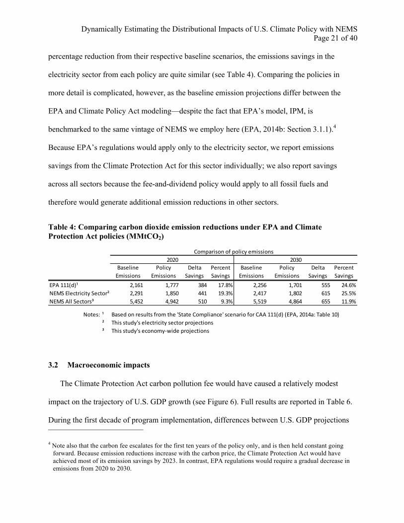
percentage reduction from their respective baseline scenarios, the emissions savings in the
electricity sector from each policy are quite similar (see Table 4). Comparing the policies in
more detail is complicated, however, as the baseline emission projections differ between the
EPA and Climate Policy Act modeling—despite the fact that EPA’s model, IPM, is
benchmarked to the same vintage of NEMS we employ here (EPA, 2014b: Section 3.1.1).4
Because EPA’s regulations would apply only to the electricity sector, we report emissions
savings from the Climate Protection Act for this sector individually; we also report savings
across all sectors because the fee-and-dividend policy would apply to all fossil fuels and
therefore would generate additional emission reductions in other sectors.
Table 4: Comparing carbon dioxide emission reductions under EPA and Climate Protection Act policies (MMtCO2)
3.2 Macroeconomic impacts
The Climate Protection Act carbon pollution fee would have caused a relatively modest
impact on the trajectory of U.S. GDP growth (see Figure 6). Full results are reported in Table 6.
During the first decade of program implementation, differences between U.S. GDP projections 4 Note also that the carbon fee escalates for the first ten years of the policy only, and is then held constant going
forward. Because emission reductions increase with the carbon price, the Climate Protection Act would have achieved most of its emission savings by 2023. In contrast, EPA regulations would require a gradual decrease in emissions from 2020 to 2030.
Baseline Emissions
Policy Emissions
Delta Savings
Percent Savings
Baseline Emissions
Policy Emissions
Delta Savings
Percent Savings
EPA 111(d)¹ 2,161 1,777 384 17.8% 2,256 1,701 555 24.6%NEMS Electricity Sector² 2,291 1,850 441 19.3% 2,417 1,802 615 25.5%NEMS All Sectors³ 5,452 4,942 510 9.3% 5,519 4,864 655 11.9%
Notes: ¹ Based on results from the 'State Compliance' scenario for CAA 111(d) (EPA, 2014a: Table 10) ² This study's electricity sector projections ³ This study's economy-‐wide projections
2020 2030Comparison of policy emissions

Dynamically Estimating the Distributional Impacts of U.S. Climate Policy with NEMS Page 22 of 40
for the baseline and the Climate Protection Act policy scenario range between 0.22% of GDP
and 0.78% of GDP. At the end of the ten-year period (in 2023), GDP is $20.5 trillion in the
reference scenario, compared with $20.4 trillion in the policy scenario. The change in GDP
represents a delay in wealth accumulation of about three months. Thus, although the emission
reductions produced by a carbon price are significant, adjustments in the economy as a whole
appear to be relatively inexpensive.
Figure 6: Impacts to U.S. GDP due to implementation of the Climate Protection Act.
3.3 Fiscal impacts
NEMS-Stanford projects that the carbon fee would raise $1.29 trillion over ten years.
Rebating 60% of the revenue would transfer $774 billion back to households. In addition, $205
billion (16%) would be allocated to policies that invest in energy efficiency in homes and
industry, job training, renewable energy, and energy research (see Table 5). The remaining $311
billion (24%) would be allocated to deficit reduction. See Table 6 for the full fiscal results.

Dynamically Estimating the Distributional Impacts of U.S. Climate Policy with NEMS Page 23 of 40
Table 5: Policy expenditures under the Climate Protection Act (billion nominal USD over a ten year horizon)
Provision Amount Purpose § 103(c)(1) $75 Cost mitigation for energy-intensive and trade-exposed industries § 103(c)(2) $50 Weatherization of low-income homes
§ 103(c)(3) $10 Job training, education, and transition assistance for former employees of fossil fuel industries
§ 103(c)(4) $20 Energy research and development (ARPA-E) § 201(e)(1) $50 Grants, loans, and loan guarantees for energy projects
One important limitation of this analysis is the simulation does not include the carbon
equivalency fee provisions (§101) aimed at imposing the carbon pollution fee on embodied
carbon in imported goods. Nor are rebates of the fee on exported fossil fuels modeled (§101).
Thus, this analysis is limited to a purely domestic perspective on fiscal impacts of the proposed
legislation.
Table 6: Environmental, macroeconomic, and fiscal results
Macroeconomic Impact Summary2013¹ 2014 2015 2016 2017 2018 2019 2020 2021 2022 2023 Total² CAGR³
Emissions price (nominal 2011 USD/tCO₂)Climate Protection Act $0.00 $20.00 $21.12 $22.30 $23.55 $24.87 $26.26 $27.73 $29.29 $30.93 $32.66 5.6%
Emissions (MMtCO₂)Reference Scenario 5369 5361 5381 5335 5367 5400 5438 5452 5452 5480 5494 54161 0.3%Climate Protection Act 5127 5039 4971 4981 5006 5012 4988 4942 4936 4919 49922 -‐0.5%∆ Emissions -‐234 -‐341 -‐365 -‐386 -‐395 -‐426 -‐464 -‐510 -‐543 -‐575 -‐4238∆ Emissions (% from Reference) -‐4.4% -‐6.3% -‐6.8% -‐7.2% -‐7.3% -‐7.8% -‐8.5% -‐9.4% -‐9.9% -‐10.5%
GDP (Billion chained 2011 USD)Reference Scenario $15,642 $16,089 $16,639 $17,149 $17,674 $18,153 $18,640 $19,112 $19,557 $20,027 $20,518 2.74%Climate Protection Act $16,054 $16,526 $17,015 $17,557 $18,065 $18,562 $19,027 $19,454 $19,906 $20,375 2.68%∆ GDP -‐$36 -‐$114 -‐$134 -‐$117 -‐$88 -‐$78 -‐$85 -‐$102 -‐$121 -‐$143∆ GDP (% from Reference) -‐0.2% -‐0.7% -‐0.8% -‐0.7% -‐0.5% -‐0.4% -‐0.4% -‐0.5% -‐0.6% -‐0.7%
Revenues (Billion nominal 2011 USD)Total $103 $106 $111 $117 $124 $132 $138 $145 $153 $161 $1,290 5.1%
notes ¹ 2013 Values are the same for Reference and policy scenario² Ten-‐year undiscounted sum total where appropriate³ Compound Annual Growth Rate
Dynamically Estimating the Distributional Impacts of U.S. Climate Policy with NEMS Page 24 of 40
3.4 Impacts to households
We calculate net benefit to household expenditures from the Climate Protection Act as
the difference between the per capita rebate and increases in cost of energy expenditure by U.S.
households. In other words, this term refers to the rebate minus the direct cost of climate policy;
to calculate the net benefit to consumer welfare, one would need to include indirect costs, which
we do not estimate here. The specified rebate level in the Climate Protection Act is 60% of
revenues. For additional context, the figures in this section also include calculations of the net
impact to household energy expenditures for lower (50%) and higher (70%) rebate levels.
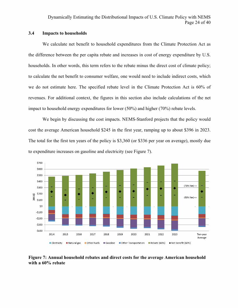
We begin by discussing the cost impacts. NEMS-Stanford projects that the policy would
cost the average American household $245 in the first year, ramping up to about $396 in 2023.
The total for the first ten years of the policy is $3,360 (or $336 per year on average), mostly due
to expenditure increases on gasoline and electricity (see Figure 7).
Figure 7: Annual household rebates and direct costs for the average American household with a 60% rebate

Dynamically Estimating the Distributional Impacts of U.S. Climate Policy with NEMS Page 25 of 40
Next, we discuss rebates. Rebating 60% of total carbon fee revenue would return $191 to
each U.S. resident in 2014, increasing to $275 by 2023. The amount returned to each household
depends on the number of people per household (PPH). According to 2011 CEX data, the
average American household had 2.5 members. Thus, the average household rebate would begin
at $478 in 2014, growing to $688 in 2023. A total of $5,744 would be rebated to the average
household over the first ten years of the policy, for an average of $574 per year.
Our analysis indicates that the Climate Protection Act would provide the average
American household with a net benefit to household energy expenditures in each of the years
studied here. The average yearly impacts are shown in the last bar of Figure 7. Over the first ten
years of the policy, the average household would experience a net reduction in direct energy
expenditures of $238 per year. The average benefit ratio is 1.71:1, with the average American
household receiving $1.71 rebate for every $1.00 spent on increased direct costs for energy-
related products and services. Again, however, we stress that these results include only the direct
cost impacts from the policy, and not the indirect costs, such as increases in the costs of non-
energy goods and services. Numerical ten-year average results are summarized at the end of this
section in Table 7.
3.4.1 Household impacts by income
Household energy expenditures vary significantly by income in the United States. Lower
income households typically spend a smaller amount on energy, but a larger fraction of their total
income. Thus, a carbon fee without a rebate is likely to have regressive impacts. By rebating a
fixed portion of carbon fee revenues back to households on a per capita basis, however, these
distributional consequences can be mitigated—and even reversed.

Dynamically Estimating the Distributional Impacts of U.S. Climate Policy with NEMS Page 26 of 40
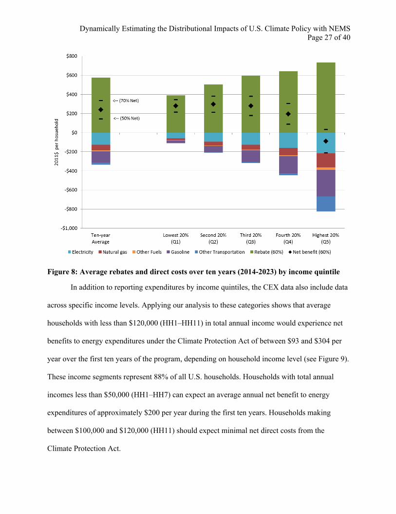
Our analysis indicates that the Climate Protection Act’s 60% rebate is sufficient to offset
increased energy prices for the lower 80% of U.S. households by income (see Figure 8). The
highest quintile of income earners faces net energy expenditure increases under the policy. Their
higher expenditures are mostly due to higher overall home energy consumption and air travel
expenditures. For U.S. households in the lower three income quintiles, the average annual net
benefit to energy expenditures from the Climate Protection Act is approximately $300 for the
first 10 years of the program. Net expenditures in the fourth quintile (Q4) would be roughly $200
on average. The fifth quintile (Q5) would have a net cost of about $90, on average, under a 60%
rebate; the net direct cost impact to Q5 would be slightly net positive under a 70% rebate.
We note that the difference in the amount rebated to average households in each quintile
is a reflection only of differences in the average PPH across incomes. On average, lower income
households tend to have fewer residents than higher income households. For example, in 2011,
the lowest 20% of U.S. households by income had 1.7 members on average, compared with 3.2
for the highest 20% (See Table 1).
Dynamically Estimating the Distributional Impacts of U.S. Climate Policy with NEMS Page 27 of 40
Figure 8: Average rebates and direct costs over ten years (2014-2023) by income quintile
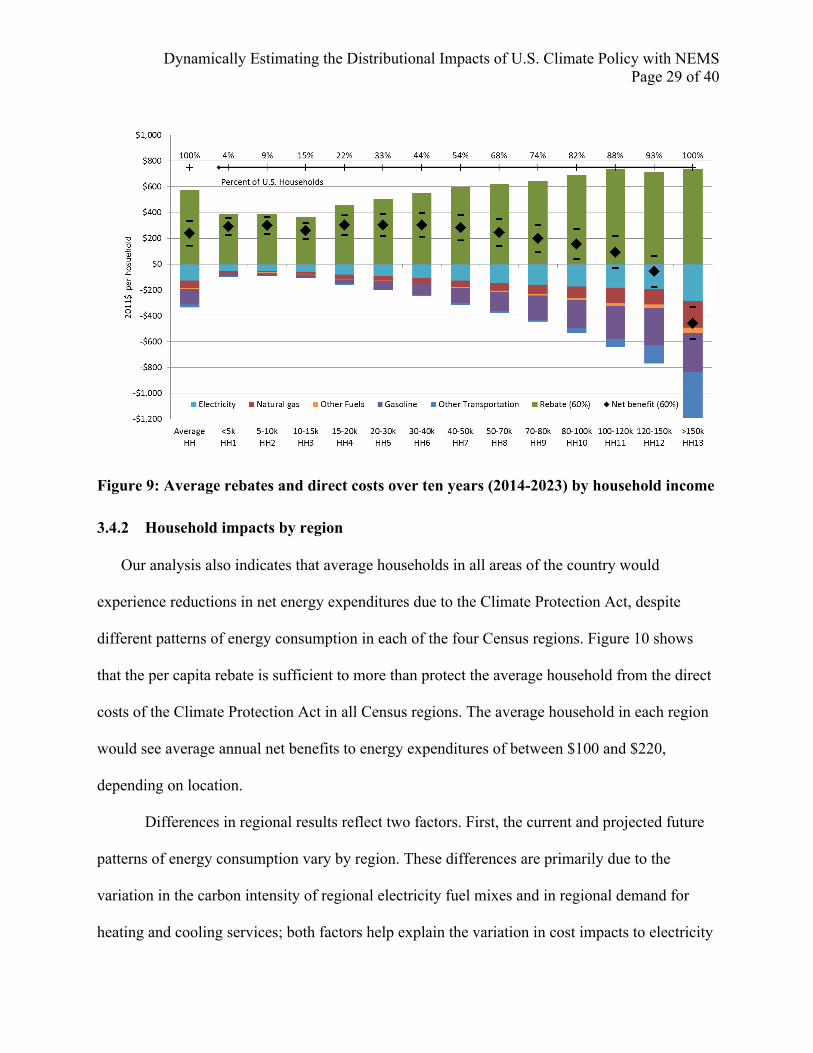
In addition to reporting expenditures by income quintiles, the CEX data also include data
across specific income levels. Applying our analysis to these categories shows that average
households with less than $120,000 (HH1–HH11) in total annual income would experience net
benefits to energy expenditures under the Climate Protection Act of between $93 and $304 per
year over the first ten years of the program, depending on household income level (see Figure 9).
These income segments represent 88% of all U.S. households. Households with total annual
incomes less than $50,000 (HH1–HH7) can expect an average annual net benefit to energy
expenditures of approximately $200 per year during the first ten years. Households making
between $100,000 and $120,000 (HH11) should expect minimal net direct costs from the
Climate Protection Act.

Dynamically Estimating the Distributional Impacts of U.S. Climate Policy with NEMS Page 28 of 40
In general, only households with total annual incomes above $120,000 (12% of all
households) should expect net increases in energy expenditures due to the direct cost of the fee-
and-dividend policy. Costs would fall most heavily on households with total annual incomes
above $150,000 (wealthiest 7% of all households). Because the wealthiest Americans consume
the most energy, due primarily to larger homes and frequent air travel, the carbon rebate does not
fully offset the increased direct costs these households would face under the Climate Protection
Act.
Under the Climate Protection Act’s 60% rebate level, the threshold for net positive
impacts to average household energy expenditures falls between HH10 and HH11
(encompassing 88% of households). Increasing the dividend percentage shifts this threshold to
the right (to include more households), while decreasing the rebate percentage shifts the
threshold to the left (to include fewer households). Under a 70% rebate, average households
earning less than $140,000 (HH1–HH12, 93% of households) would experience net benefits to
energy expenditures. Under a 50% rebate, average households earning less than $100,000 (HH1–
HH10, 82% of households) would experience net benefits to energy expenditures.
Dynamically Estimating the Distributional Impacts of U.S. Climate Policy with NEMS Page 29 of 40
Figure 9: Average rebates and direct costs over ten years (2014-2023) by household income
3.4.2 Household impacts by region
Our analysis also indicates that average households in all areas of the country would
experience reductions in net energy expenditures due to the Climate Protection Act, despite
different patterns of energy consumption in each of the four Census regions. Figure 10 shows
that the per capita rebate is sufficient to more than protect the average household from the direct
costs of the Climate Protection Act in all Census regions. The average household in each region
would see average annual net benefits to energy expenditures of between $100 and $220,
depending on location.
Differences in regional results reflect two factors. First, the current and projected future
patterns of energy consumption vary by region. These differences are primarily due to the
variation in the carbon intensity of regional electricity fuel mixes and in regional demand for
heating and cooling services; both factors help explain the variation in cost impacts to electricity

Dynamically Estimating the Distributional Impacts of U.S. Climate Policy with NEMS Page 30 of 40
and natural gas expenditures. Second, dividend benefits vary due to minor regional differences in
average household size.
Figure 10: Estimated average rebates and direct costs for average households by region, 2014-2023

Dynamically Estimating the Distributional Impacts of U.S. Climate Policy with NEMS Page 31 of 40
Table 7: Summary of average annual rebates and direct costs for each market segment.
4. Discussion
The most important caveat to our distributional analysis is that we examine only the
direct policy costs and lump sum rebates under a prospective climate policy. Our analysis does
not incorporate the losses to GDP projected by NEMS-Stanford, nor does it include any other
measure of indirect costs or benefits. As explained below, GDP losses are likely overstated.
Nevertheless, our analysis excludes other indirect costs that households would face, including
Natural Gas
ElectricityFuel oil & Other Fuel
Gasoline & Motor Oil
Other Trans.
Total Cost
Rebate (60%)
Net Change
Percent of income²
Mkt. Seg. Cum.
Average Household$59.43 $126.03 $9.02 $118.37 $23.01 $335.86 $574.39 $238.53 0.4% 100.0% -‐
By Income Quintiles$19.89 $60.39 $2.65 $25.28 $2.86 $111.07 $390.59 $279.52 2.8% 20% 20.0%$38.49 $94.77 $5.18 $65.90 $3.60 $207.95 $505.46 $297.52 1.1% 20% 40.0%$50.20 $127.09 $7.18 $121.88 $11.64 $317.98 $597.37 $279.39 0.6% 20% 60.0%$75.06 $159.93 $10.58 $182.32 $19.50 $447.38 $643.32 $195.94 0.3% 20% 80.0%$146.31 $216.01 $26.69 $278.58 $157.94 $825.54 $735.22 -‐$90.32 -‐0.1% 20% 100.0%
By Region$0.00 $84.04 $22.68 $105.41 $31.11 $243.24 $551.42 $308.18 0.4% 18.4% -‐$90.20 $129.29 $9.19 $116.15 $19.40 $364.22 $551.42 $187.19 0.3% 22.2% -‐$32.46 $173.48 $18.88 $131.59 $15.27 $371.68 $574.39 $202.71 0.4% 36.7% -‐$62.07 $78.02 $3.72 $108.65 $32.03 $284.49 $597.37 $312.88 0.5% 22.7% -‐
By Household Income$19.57 $51.43 $0.88 $22.13 $4.61 $98.62 $390.59 $291.97 N/A⁴ 4.1% 4.1%$13.61 $50.41 $3.66 $20.77 $2.13 $90.58 $390.59 $300.01 3.7% 4.5% 8.5%$17.67 $62.99 $2.77 $23.07 $2.59 $109.08 $367.61 $258.53 2.0% 6.7% 15.2%$33.64 $79.05 $4.67 $37.13 $2.71 $157.21 $459.51 $302.31 1.7% 6.3% 21.5%$35.37 $91.88 $6.38 $65.24 $3.05 $201.92 $505.46 $303.55 1.2% 11.8% 33.4%$46.37 $105.51 $3.44 $84.79 $6.87 $246.98 $551.42 $304.43 0.9% 10.9% 44.3%$48.65 $127.81 $7.38 $120.52 $10.17 $314.53 $597.37 $282.84 0.6% 9.3% 53.5%$61.43 $143.04 $9.14 $147.23 $14.45 $375.29 $620.34 $245.05 0.4% 14.2% 67.8%$71.91 $159.33 $10.46 $187.90 $15.75 $445.35 $643.32 $197.97 0.3% 6.0% 73.8%$91.80 $171.92 $12.80 $219.09 $37.64 $533.25 $689.27 $156.02 0.2% 8.6% 82.3%$122.50 $181.99 $19.03 $258.18 $60.39 $642.09 $735.22 $93.13 0.1% 5.8% 88.1%$120.48 $192.79 $26.10 $289.22 $140.02 $768.61 $712.25 -‐$56.36 0.0% 5.0% 93.1%$204.45 $286.89 $40.11 $305.75 $355.02 $1,192.23 $735.22 -‐$457.01 -‐0.2% 6.9% 100.0%
Notes: ¹ Based on ten-‐year average results² Based on average after-‐tax income from CEX for each market segment³ First column is percent for each market segment, the second is cumulative, ordered from lowest income segment⁴ Income for HH1 is negative, so expressing the net policy impacts to expenditures as a % of income is not logical
$120k to <$150k (HH12)$150k and more (HH13)
Average Direct Costs
$30k to <$40k (HH6)$40k to <$50k (HH7)$50k to <$70k (HH8)$70k to <$80k (HH9)$80k to <$100k (HH10)
Market Segment
Average Anmnual Policy impacts to household market segments¹
Midwest (MW)South (S)West (W)
Avg. Consumer Unit
Lowest 20% (Q1)Second 20% (Q2)
$20k to <$30k (HH5)
Highest 20% (Q5)
Northeast (NE)
Fourth 20% (Q4)
$100k to <$120k (HH11)
Percent of HH³
Less than $5k (HH1)$5k to <$10k (HH2)$10k to <$15k (HH3)$15k to <$20k (HH4)
Rebate and Net Change
Third 20% (Q3)

Dynamically Estimating the Distributional Impacts of U.S. Climate Policy with NEMS Page 32 of 40
changes in the cost of goods and services due to the increased cost of embodied energy
throughout the economy.
We chose to focus exclusively on household energy expenditures because these could be
mapped to corresponding NEMS outputs. By linking energy expenditures to an energy-economy
model with microeconomic and macroeconomic effects, we are able to more accurately estimate
the changes to energy expenditures. Indeed, we aim to contribute to climate policy discussions
by offering a dynamic method to study the direct costs of climate policy. In order to assess the
full impact on consumer welfare, however, these direct costs must be augmented by reliable
estimates of indirect costs.
We note that indirect cost estimates generally suffer from the challenge of projecting how
the mixture of general goods and services in the economy would respond to a price on carbon.
Depending on the household income level in question, other researchers estimate that average
indirect costs could range from an additional 50% to 100% of the direct costs (e.g., Hassett et al.,
2009; Mathur and Morris, 2014). Due to the complexity of the calculations, however, most
assessments of indirect costs are made using static assumptions about household consumption of
goods and services. As a result, they do not account for dynamic effects—including, most
importantly, the likelihood that consumers and firms would change their consumption patterns in
response to higher energy costs. Studies that assume no change in consumption are likely to
overestimate indirect costs, though of course including some estimate of indirect cost is
necessary to assessing the full effect of climate policy on consumer welfare.
One can combine direct and indirect costs to yield an estimate of total policy costs, but
this must be done carefully. If indirect costs for average households are well approximated by
Mathur and Morris (2014), then our results suggest that the average change in consumer welfare

Dynamically Estimating the Distributional Impacts of U.S. Climate Policy with NEMS Page 33 of 40
from the Climate Protection Act could range between a net benefit of $70 a year to a net cost of
$97 per year for the average household (for indirect costs of an additional 50% and 100% of
direct costs, respectively). We caution readers that it is inappropriate to apply average indirect
costs when extrapolating across household income levels, however, as Mathur and Morris report
a strong correlation between household income and indirect costs.
Furthermore, our projected impacts to GDP are very likely overstated for two reasons.
First, the impacts of policies aimed at reducing energy-related carbon emissions that are funded
by the Climate Protection Act (§§103, 201) are not included. Second, no attempt is made to
account for the welfare impacts of changed environmental externalities under the policy. We
neglect both global climate benefits and national public health benefits. On the climate benefits,
the U.S. government’s social cost of carbon (Interagency Working Group, 2013) estimates the
total global externality impacts from carbon pollution. But climate benefits are often much
smaller than improvements in U.S. public health and healthcare costs associated with reduced air
pollution. Prominent economists recently concluded that air pollution damages from some
industries, such as coal-fired power plants, are greater than the amount those industries
contribute to GDP (Muller et al., 2011). This finding is particularly important here, as our results
show that the Climate Protection Act would reduce emissions primarily by switching from coal-
fired electricity generation to natural gas-fired and renewable generation. Thus, our results
include the costs of choosing cleaner energy, but not the tangible benefits to the global
environment or to public health in the United States that come from reducing our consumption of
high-polluting coal power. As a final example of the importance of health impacts, we note that
EPA’s cost-benefit analysis of its forthcoming Clean Air Act § 111(d) regulations shows that

Dynamically Estimating the Distributional Impacts of U.S. Climate Policy with NEMS Page 34 of 40
expected health benefits alone were more than sufficient to justify the costs of the regulations
(EPA, 2014a: Tables 18-21).
Two additional reasons suggest GDP is overstated, but are less important in this context.
First, the projected impacts to GDP are limited by the core assumptions in NEMS. Notably, the
model does not fully account for the possibility of induced innovation, which some believe a
carbon price on carbon would encourage. Environmental economists have shown that induced
innovation in the context of climate policy has the potential to significantly lower compliance
costs and increase social welfare (Goulder and Mathai, 2000). We merely note the issue here
without assessing whether carbon prices in the range of those imposed by the Climate Protection
Act would be sufficient to cause these changes. Second, the structure of the macroeconomic
model does not account for any impacts of deficit reduction under the Climate Protection Act on
future U.S. debt servicing costs.
Finally, our analysis is based entirely on the structure of NEMS. Any bias that is in the
model structure, code, or standard input parameters will be reflected in our results.
5. Conclusions
In this paper, we describe a methodology for dynamically estimating the direct costs of
climate policy across U.S. households of different income levels and different regions. Our
approach combines output from an independent copy of the federal government’s flagship
energy-economic model (NEMS-Stanford) with cross-sectional data on household expenditures
(CEX). We then apply our methodology to analyze S. 332, the Boxer-Sanders Climate Protection
Act of 2013, which would have implemented a fee-and-dividend policy in the U.S.
Dynamically Estimating the Distributional Impacts of U.S. Climate Policy with NEMS Page 35 of 40
The Climate Protection Act would have levied a carbon pollution fee on energy-related
carbon dioxide (CO2) emissions, starting in 2014 at $20 per metric ton of CO2 and rising at 5.6%
in nominal terms each year through 2023. We estimate that the bill would have raised $1.3
trillion in carbon revenues over its first ten years. A fixed portion would be rebated to American
households on a per capita basis ($774 billion, or 60%). Additional expenditures ($205 billion, or
16%) would be used to assist trade-exposed industries, weatherize low-income households,
retrain and compensate displaced workers, increase energy R&D, and support new energy
project finance. The remaining revenues ($311 billion, or 24%) would be used to reduce the
federal government’s deficit.
NEMS-Stanford projects that the policy would have reduced energy-related CO2
emissions by 4,200 million metric tonnes in the first ten years of the program. These reductions
represent an 8.5% decline from baseline emissions in 2010 and a 10.5% decline in 2023. Our
projections also indicate that energy-related CO2 emissions would have fallen 17% below 2005
levels in 2020, putting the United States within reach of its commitment to reduce under the
Copenhagen Accord. Finally, we find that the emission reductions from this policy would occur
more rapidly than those projected by EPA’s analysis of its proposed Clean Air Act § 111(d)
regulations.
NEMS-Stanford projects modest impacts to GDP of less than one half of one percent in
2020. These impacts are likely overstated, however, as our modeling framework does not
account for environmental externalities, cost containment from complementary policy measures,
fiscal stimulus effects, or deficit reductions. We note that the dominant source of emission
reductions in the policy scenario comes from switching between coal- and natural gas-fired
power plants. Because the environmental externalities from coal power plant production have

Dynamically Estimating the Distributional Impacts of U.S. Climate Policy with NEMS Page 36 of 40
been shown to exceed their contribution to GDP, due to the tangible public health costs from air
pollution, this suggests that our macroeconomic costs are overstated.
To explore the distributional consequences of the policy across households of different
income levels and in different areas of the country, we coupled NEMS-Stanford output with the
Bureau of Labor Statistics’ 2011 Consumer Expenditure Survey (CEX). By linking the energy-
related expenditures in the CEX to corresponding data series projected by NEMS-Stanford, we
dynamically estimated the increased energy costs households of different income levels and in
different regions of the country would experience under the Climate Protection Act. We included
a household-level calculation of the per capita climate dividend to estimate the net impact on
household energy expenditures—i.e., the value of the climate dividend minus the policy’s direct
costs. Based on this analysis, we find that the policy would reduce net energy-related
expenditures for average households making less than $120,000 per year (the bottom 88% by
income). It would also reduce net energy-related expenditures for the average U.S. household in
all regions of the country. A sensitivity analysis shows how these thresholds change if the rebate
were increased to 70% of revenue or decreased to 50%.
Overall, these results suggest that a fee-and-dividend policy can be designed to protect a
wide range of household income levels from direct energy costs while also using the remaining
revenue for deficit reduction or other policy expenditures. Such a policy can also drive relatively
rapid emissions reductions that enable the U.S. to meet its obligations under the Copenhagen
Accord. In order to fully evaluate the consumer welfare implications of U.S. climate policy,
however, our reported direct policy costs should be supplemented with other estimates of indirect
policy costs.

Dynamically Estimating the Distributional Impacts of U.S. Climate Policy with NEMS Page 37 of 40
Acknowledgments
We thank the following Stanford University groups for their financial support: the Precourt
Institute for Energy, Steyer-Taylor Center for Energy Policy and Finance, Energy Modeling
Forum, and School of Earth Sciences.
Dynamically Estimating the Distributional Impacts of U.S. Climate Policy with NEMS Page 38 of 40
References
Blonz, J., Burtraw, D., Walls, M.A., 2011. How Do the Costs of Climate Policy Affect Households? The Distribution of Impacts by Age, Income, and Region (No. DP 10-55), RFF Discussion Paper. Washington, DC.
BLS, 2013. Consumer Expenditures in 2011. Report 1042, U.S. Bureau of Labor Statistics, Washington D.C.
Boxer, B., Sanders, B., 2013. The Climate Protection Act (S. 332) [WWW Document]. URL https://www.govtrack.us/congress/bills/113/s332/text
Brown, M.A., Baek, Y., 2010. The forest products industry at an energy/climate crossroads. Energy Policy 38, 7665–7675. doi:10.1016/j.enpol.2010.07.057
Brown, M.A., Levine, M.D., Short, W., Koomey, J.G., 2001. Scenarios for a clean energy future. Energy Policy 29, 1179–1196.
CBO, 2009. The Role of the 25 Percent Revenue Offset in Estimating the Budgetary Effects of Proposed Legislation. Washington, D.C.
Chandel, M.K., Pratson, L.F., Jackson, R.B., 2011. The potential impacts of climate-change policy on freshwater use in thermoelectric power generation. Energy Policy 39, 6234–6242. doi:10.1016/j.enpol.2011.07.022
Choi Granade, H., Creyts, J., Derkach, A., Farese, P., Nyquist, S., Ostrowski, K., 2009. Unlocking Energy Efficiency in the U.S. Economy: Executive Summary. McKinsey & Company Report.
Creyts, J., Derkach, A., Nyquist, S., Ostrowski, K., Stephenson, J., 2007. Reducing U.S. Greenhouse Gas Emissions: How Much and at What Cost? US Greenhouse Gas Abatement Mapping Initiative, Executive Report. McKinsey and Company.
EIA, 1998. Impacts of the Kyoto Protocol on U.S. Energy Markets and Economic Activity. Washington DC.
EIA, 2008a. Energy Market and Economic Impacts of S. 2191, the Lieberman-Warner Climate Security Act of 2007. US Department of Energy, Energy Information Administration, Washington, DC.
EIA, 2008b. Energy Market and Economic Impacts of S. 1766, the Low Carbon Economy Act of 2007. US Department of Energy, Energy Information Administration, Washington, DC.
EIA, 2009a. Energy Market and Economic Impacts of H . R . 2454 , the American Clean Energy and Security Act of 2009. Washington D.C.

Dynamically Estimating the Distributional Impacts of U.S. Climate Policy with NEMS Page 39 of 40
EIA, 2009b. The National Energy Modeling System: An Overview. US Department of Energy, Energy Information Administration, Washington, DC.
EIA, 2010a. Energy Market and Economic Impacts of the American Power Act of 2010. US Department of Energy, Energy Information Administration, Washington, DC.
EIA, 2010b. Energy Market and Economic Impacts of the Carbon Limits and Energy for America ’ s Renewal ( CLEAR ) Act and an Electric-Power Only Cap-and-Trade Program. Washington, D.C.
EIA, 2010c. Integrating Module of the National Energy Modeling System : Model Documentation 2013, OAIF. EIA, Washington, D.C.
EIA, 2012a. Annual Energy Outlook 2012 with projections to 2035. Washington, D.C.
EIA, 2012b. U.S. Greenhouse Gas Emissions and Sinks: 1990-2010. Washington, D.C.
EIA, 2013a. Model Documentation Report : Macroeconomic Activity Module (MAM) of the National Energy Modeling System. Washington, D.C.
EIA, 2013b. Annual Energy Outlook 2013 with projections to 2040. Washington, D.C.
EPA, 2014a. Carbon Pollution Emission Guidelines for Existing Stationary Source: Electric Utility Generating Units; Proposed Rule. Federal Register 79(117): 34830-34958.
EPA, 2014b. Regulatory Impact Analysis for the Proposed Carbon Pollution Guidelines for Existing Power Plants and Emission Standards for Modified and Reconstructed Power Plants. Report # EPA-542/R-14-002 [WWW Document]. URL http://www2.epa.gov/carbon-pollution-standards/clean-power-plan-proposed-rule
Fawcett, A.A., Clarke, L.E., Rausch, S., Weyant, J.P., 2014. Overview of EMF 24 Policy Scenarios. Energy J. 35, 33–60.
Goulder, L.H., 2013. Climate change policy’s interactions with the tax system. Energy Econ. 40, S3–S11. doi:10.1016/j.eneco.2013.09.017
Goulder, L.H., Hafstead, M.A.C., 2013. Tax Reform and Environmental Policy: Options for Recycling Revenue from a Tax on Carbon Dioxide, RFF Discussion Paper 13-31. Washington, D.C.
Goulder, L.H., Mathai, K., 2000. Optimal CO2 Abatement in the Presence of Induced Technological Change. J. Environ. Econ. Manage. 39, 1–38. doi:10.1006/jeem.1999.1089
Hassett, K.A., Mathur, A., Metcalf, G.E., 2009. The Incidence of a U.S. Carbon Tax: A Lifetime and Regional Analysis. Energy J. 30(2), 155–177. doi:10.5547/ISSN0195-6574-EJ-Vol30-No2-8

Dynamically Estimating the Distributional Impacts of U.S. Climate Policy with NEMS Page 40 of 40
Houser, T., Mohan, S., 2014. Fueling Up: The Economic Implications of America’s Oil & Gas Boom. Peterson Institute for International Economics, Washington D.C.
Interagency Working Group, 2013. Technical Support Document: Technical Update of the Social Cost of Carbon for Regulatory Impacts Analysis Under Executive Order 12866.
Kydes, A.S., 2007. Impacts of a renewable portfolio generation standard on US energy markets. Energy Policy 35, 809–814.
Luong, T., Murphy, F.H., Sanders, R., Holte, S.H., Loring, D., 1998. Modeling the Impacts of the 1990 Clean Air Act Amendments. Interfaces (Providence). 28, 1–15.
Mathur, A., Morris, A.C., 2014. Distributional effects of a carbon tax in broader U.S. fiscal reform. Energy Policy 66, 326–334. doi:10.1016/j.enpol.2013.11.047
Metcalf, G.E., 1999. A Distributional Analysis of Green Tax Reforms A Distributional Analysis of. Natl. Tax J. 52, 655–682.
Metcalf, G.E., 2009. Designing a Carbon Tax to Reduce U.S. Greenhouse Gas Emissions. Rev. Environ. Econ. Policy 3, 63–83. doi:10.1093/reep/ren015
Morrow, R.W., Gallagher, K.S., Collantes, G., Lee, H., 2010. Analysis of policies to reduce oil consumption and greenhouse-gas emissions from the US transportation sector. Energy Policy 38, 1305–1320. doi:10.1016/j.enpol.2009.11.006
Muller, N.Z., Mendelsohn, R., Nordhaus, W., 2011. Environmental Accounting for Pollution in the United States Economy. Am. Econ. Rev. 101, 1649–1675.
UNFCCC, 2010. Report of the Conference of the Parties on its fifteenth session.
Wilkerson, J.T., 2014. Economic and Distributional Impacts from Carbon Fee and Dividend Policies. Doctoral Thesis. Management Science & Engineering (MS&E). Stanford University, Palo Alto, CA.
Wilkerson, J.T., Cullenward, D., Davidian, D., Weyant, J.P., 2013. End use technology choice in the National Energy Modeling System (NEMS): An analysis of the residential and commercial building sectors. Energy Econ. 40, 773–784. doi:10.1016/j.eneco.2013.09.023
Williams, R.C.I., Gordon, H., Burtraw, D., Carbone, J.C., Morgenstern, R.D., 2014. The Initial Incidence of a Carbon Tax across US States (No. RFF DP 14-25), RFF Discussion Paper. Washington, D.C.