Dynamical Model of Rocket Propellant Loadingwith Liquid Hydrogen

Viatcheslav V. Osipov!

MCT, Inc., Moffett Field, California 94035Matthew J. Daigle†

University of California, Santa Cruz, Moffett Field, California 94035Cyrill B. Muratov‡

New Jersey Institute of Technology, Newark, New Jersey 07102Michael Foygel§

SGT, Inc., Newark, New Jersey 07102Vadim N. Smelyanskiy¶

NASA Ames Research Center, Moffett Field, California 94035and

Michael D. Watson!!

NASA Marshall Space Flight Center, Huntsville, Alabama 35805

DOI: 10.2514/1.52587

Adynamical model describing themultistage process of rocket propellant loading has been developed. It accountsfor both the nominal and faulty regimes of cryogenic fuel loadingwhen liquid hydrogen ismoved from a storage tankto an external tank via a transfer line. By employing basic conservation laws, the reduced lumped-parameter modeltakes into consideration the major multiphase mass and energy exchange processes involved, such as highlynonequilibrium condensation–evaporation of hydrogen, pressurization of the tanks, and liquid hydrogen andhydrogenvaporflows in the presence of pressurizing heliumgas.A self-consistent theory of dynamical condensation–evaporation has been developed that incorporates heat flow by both conduction and convection through the liquid/vapor interface inside the tanks. A simulation has been developed in MATLAB for a generic refueling system thatinvolves the solution of a system of ordinary integro-differential equations. The results of these simulations are ingood agreement with space shuttle refueling data.

NomenclatureA = cross-sectional area of storage tank, pipe, or liquid/

vapor interface in storage tank, m2

cP!V" = constant pressure (volume) specific heat, J=K # kgdr = wall roughness, mf = dimensionless resistance coefficientH = height of external tank, mh = specific enthalpy, J=kghl = height (level) of liquid, mJ = gas/vapor or liquid-mass flow rate, kg=sK = dimensionless loss factorl = pipe length; mm = mass of control volume, kg

Nu, Ra,Re, Pr

= dimensionless Nusselt, Rayleigh, Reynolds, andPrandtl numbers

p = (partial) pressure, Pa_Q = heat flow rate from or to control volume, WR = radius of external tank, storage tank, or pipe, mRv, Rg = LH2 and gaseous He gas constants, J=K # kgS = cross-sectional area of vent valve area or leak

hole, m2

T = temperature, Ku = specific internal energy, J=kgV = volume, m3

v = velocity of liquid/vapor in pipes or valves, m=s_W = power on or by control volume, w! = convection heat transfer coefficient, W=m2 # K" = ratio of specific heats, cP=cV# = thermal conductivity,W=m # K$ = dimensionless vent valve position% = dynamic viscosity, kg=m # s& = kinematic viscosity, m2=s' = density, kg=m3

( = dimensionless multiplicative clogging factor) = time constant of vaporizer valve or transfer line, s

Subscripts

a = ambientboil = vapor generated by vaporizerC = critical pointe = external heat or mass flows across control volume

boundaries other than liquid/vapor interfacef = gaseous hydrogen vapor filmg = gaseous heliuml = liquid hydrogen

Received 8 October 2010; revision received 18 March 2011; accepted forpublication 26 March 2011. This material is declared a work of the U.S.Government and is not subject to copyright protection in the United States.Copies of this paper may be made for personal or internal use, on conditionthat the copier pay the $10.00 per-copy fee to theCopyright Clearance Center,Inc., 222RosewoodDrive, Danvers,MA01923; include the code 0022-4650/11 and $10.00 in correspondence with the CCC.

!Leading Researcher; Federal Contractor, NASA Ames Research Center,Applied Physics Group, Moffett Field, CA 94035.

†Associate Scientist, Intelligent Systems Division; Federal Contractor,NASA Ames Research Center, Applied Physics Group, Moffett Field, CA94035. Member AIAA.

‡Associate Professor, NASA Ames Research Center, Department ofMathematical Sciences, Moffett Field, CA 94035.

§Research Scientist; Federal Contractor, NASA Ames Research Center,Applied Physics Group, Moffett Field, CA, 94035.

¶Senior Research Scientist, Applied Physics Group Lead; FederalContractor, NASA Ames Research Center, Applied Physics Group, MoffettField, CA 94035.

!!Chief, ISHM and Sensors Branch.

JOURNAL OF SPACECRAFT AND ROCKETSVol. 48, No. 6, November–December 2011

987

ls = saturated liquidlv = liquid/vapor phase transitionS = liquid/vapor interfacetr = transfer linev = gaseous hydrogen vaporvap = vaporizervs = saturated vaporw = tank wallw=boil = vapor generated by tank walls

I. Introduction

T HE fueling of rockets with liquid propellant is a very importantand dangerous procedure, especially in the case of hydrogen [1–

4]. The major goal of this paper is to develop a medium-fidelitylumped-parameter dynamical model of propellant loading that1) takes into consideration a variety of complex multiphase phe-nomena that govern the storage and transfer of cryogenic propellants,and yet is simple enough to 2) allow for physics analysis and issuitable for numerical simulations of real loading systems. Withrelatively small modifications, the proposed model can be applied tothe description of onground loading of different cryogenic pro-pellants and account for thermal stratification in the ullage regions ofthe tanks. In this paper, we concentrate on a system of liquidhydrogen (LH2) filling motivated by the parameters of the spaceshuttle refueling system. Such a system can be considered as genericwith respect tomany existing and emerging liquid propellant loadingschemes and cryogenic fluid management technologies.

The purpose of the LH2 propellant loading system is tomove LH2from the storage tank (ST) to the external tank (ET) (see Fig. 1). LH2is stored on the ground in a spherical, insulated double-walled STwith a radius of about 10 m. The height of the ET is about 30 m. Thecorresponding hydrostatic pressures of liquid hydrogen near thebottoms of the tanks are much less than the saturated vapor pressuresat the operating temperature. Therefore, a high operating pressure isneeded to suppress potential boiling of the liquid hydrogen. Toensure such pressure, helium gas is injected into the ET, and pressureis maintained throughout filling with the help of a vent valve. In theST, a vaporizer is used to maintain the ullage pressure by producinggaseous hydrogen (GH2). It is kept at a higher pressure than in theET, such that the transfer of LH2 from the ST into the ET isaccomplished.

An accurate model of this system is needed for supporting loadingprocedure optimization analyses and ensuring system safety throughmodel-based fault diagnostic and prognostic algorithms. However,developing such a model, especially one that is simple yet accurateenough for these purposes, is challenging: although complex physicsphenomena govern the flow of the cryogenic propellants, onlylimited data are available to validate models. The processes of heattransfer and phase change prove to be central to the understanding ofthe loading system and its correct functioning [1,4]. In [1], whiledescribing a cryogenic (external) tank history, Estey et al. took into

consideration heat transfer by convection only. In some cases,however, the heat transfer by conduction is essential in the treatmentof the heat and mass flow across the LH2/GH2 boundary leading tothe so-called condensation blocking [4]. The latter effect is shown [4]to be essential to the consistent description of the cryogenic tankhistory.

The paper is organized in the followingway. In Sec. II, we considerthe nonequilibriumdynamics of condensation–evaporation at (and ofthe heat flow through) the liquid/vapor interface. Section III dealswith a consistent description of the cryogenic tank’s history. Itincorporates the analysis of the propellant mass flow in the transferline (TL), which is critical to an adequate modeling of the nominaland faulty regimes of the rocket propellant loading, described inSecs. IVandV, respectively. In Sec. VI, themodel is validated againstdata collected from a real rocket cryogenic (LH2) propellant loadingsystem. Section VII concludes the paper.

II. Condensation–Evaporation and HeatFlow Processes

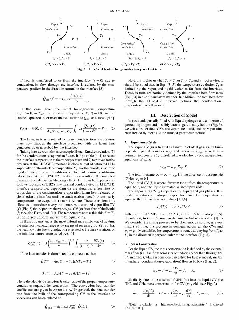
We begin with a general description of the condensation–evaporation and heatflow,which occurs at the LH2/GH2 interface, asthese processes form the core of the propellant loadingmodel. If, in atank partially filled by a cryogenic propellant, the liquid phase is inthermodynamic equilibrium with the vapor phase above it, then thetemperature profile is uniform across the interface. The mass flowrate due to condensation Jc is balanced by the evaporation mass flowrate Jd so that both the net mass flow rate Jlv $ Jc % Jd from thevapor control volume (CV) to the liquid CVand the heatflow throughthe liquid/vapor interface disappear. When the tank is being filled oremptied, Jlv " 0. As evaporation is accompanied by heat removal, itleads to cooling of the interface, while condensation results in itsheating. Therefore, in nonequilibrium conditions the interfacetemperature TS differs from that of the bulk liquid Tl and that of thevapor Tv, resulting in temperature gradients in both the liquid andvapor volumes adjacent to the interface, as shown in Fig. 2, in whichpossible operational modes are indicated that can be responsible forthe shown sequence of temperatures, and positive external flow ratesJel!v" correspond to mass entering CV l!v". In turn, these gradientswill generate nonvanishing heat fluxes _Qv and _Ql across theinterface. Depending on the situation, these fluxes can be associatedwith heat transfer due to conduction or natural convection [4].

Our estimates show that if the processes involved vary slowly overtimescales exceeding 0.1 s, then the natural convection, if present,dominates the heat conduction inGH2 at low temperatures. (The heattransfer from the tank walls will further facilitate the effect ofconvection.) Then, taking into consideration that natural convectioncan occur if the lower part of a CV (liquid or vapor) is hotter than theupper one, we have derived the classification of temperaturegradients and of the heat transfer regimes in the vicinity of the liquid/vapor interface, shown in Fig. 2.

Fig. 1 LH2 propellant loading schematic.

988 OSIPOV ETAL.

If heat is transferred to or from the interface (x$ 0) due toconduction, its flow through the interface is defined by the tem-perature gradient in the direction normal to the interface [5]:

_Q l!v"!t" $ %#l!v"A@!!x; t"@x

!!!!x$0

(1)

In this case, given the initial homogeneous temperature!!x; t$ 0" $ Tl!v", the interface temperature TS!t" $!!x$ 0; t"can be expressed in terms of the heat flow rate _Ql!v" as follows [4,5]:

TS!t" $!!0; t" $ 1

A""""""""""""""""""""""""""""*cl!v"'l!v"#l!v"p

Zt

0

d)_Ql!v"!)"!t % )"1=2 & Tl!v" (2)

The latter, in turn, is related to the net condensation–evaporationmass flow through the interface associated with the latent heatgenerated at, or absorbed by, the interface.

Taking into account the microscopic Hertz–Knudsen relation [5]for the condensation–evaporation fluxes, it is possible [4] 1) to relatethe interface temperature to the vapor pressure and 2) to prove that thepressure at the LH2/GH2 interface is close to that of saturated LH2vapor taken at the interface temperatureTS. In otherwords, in spite ofhighly nonequilibrium conditions in the tank, quasi equilibriumtakes place at the LH2/GH2 interface as a result of the so-calleddynamical condensation blocking effect [4]. It can be explained asfollows. Because of LH2’s low thermal conductivity, the LH2/GH2interface temperature, depending on the situation, either rises ordrops due to the condensation–evaporation latent heat released orabsorbed at the interface until the condensation mass flow rate nearlycompensates the evaporation mass flow rate. These considerationsallow us to introduce a very thin, massless, saturated vapor film CV(f) (Fig. 2) that separates the vapor/gas CV (v) from that of the liquid(l) (see also Estey et al. [1]). The temperature across this thin film Tfis considered uniform and set to be equal to TS.

In these circumstances, themost natural and simpleway of treatingthe interface heat exchange is by means of reversing Eq. (2), so thatthe heat flow rate due to conduction is related to the time variations ofthe interface temperature as follows [5]:

_Q condl!v" !t" $ A

##l!v"cl!v"'l!v"

*

$1=2Zt

0

d)

!t% )"1=2@TS!)"@)

(3)

If the heat transfer is dominated by convection, then

_Q convv $ A!v!TS % Tv"H!TS % Tv" (4)

_Q convl $ A!l!Tl % TS"H!Tl % TS" (5)

where the Heaviside functionH takes care of the proper temperatureconditions required for convection. (The convection heat transfercoefficients are given in Appendix A.) In general, the heat transferrate from the bulk of the corresponding CV to the interface orvice versa can be calculated as

_Q l!v" $ 'maxf _Qcondl!v" ; _Q

convl!v" g (6)

Here, a& is chosenwhenTv > TS orTS > Tl, and a% otherwise. Itshould be noted that, in Eqs. (3–5), the temperature evolution TS isdefined by the vapor and liquid variables far from the interface.These, in turn, are partially defined by the interface heat flow rates[Eq. (6)] in a self-consistent manner. In addition, the total heat flowthrough the LH2/GH2 interface defines the condensation–evaporation mass flow rate.

III. Description of ModelIn each tank partially filled with liquid hydrogen and a mixture of

gaseous hydrogen and possibly another gas, usually helium (Fig. 3),we will consider three CVs: the vapor, the liquid, and the vapor film,each treated by means of the lumped-parameter method.

A. Equations of State

The vapor CV (v) is treated as a mixture of ideal gases with time-dependent partial densities 'v!g" and pressures pv!g", as well as acommon temperatureTv, all related to each other by two independentequations of state:

pv!g" $ 'v!g"Rv!g"Tv (7)

The total pressure pt $ pv & pg. [In the absence of gaseous He(GHe), 'g $ 0.]

The liquid CV (l) is where, far from the surface, the temperature isequal to Tl and the liquid is treated as incompressible.

The vapor film CV (f) separates the liquid and gas phases. It istreated as saturated hydrogen vapor, for which the temperature isequal to that of the interface, where [1,4,6]

pf!Tf" $ pC!Tf=TC"n (8)

with pC $ 1:315 MPa, TC $ 33:2 K, and n$ 5 for hydrogen [6].(To relatepf toTf $ TS, one can also use theAntoine equation [7].††)We consider the filling process to be slow enough so that, at everyinstant of time, the pressure is constant across all the CVs andpv $ pf. Meanwhile, the temperature is treated as varying from Tl toTv in the direction x perpendicular to the interface (Fig. 2).

B. Mass Conservation

For the liquid CV, the mass conservation is defined by the externalmass flow (i.e., the flow across its boundaries other than through thev=l interface), which is considered negative forfluid removal, and theinterphase (condensation–evaporation) flow as follows (Fig. 2):

_m l $ Jl $ 'ldVldt$ Jle & Jlv (9)

Similarly, due to the absence of GHe flux into the liquid CV, theGH2 and GHe mass conservation for CV (v) yields (see Fig. 2)

_m v $d!'vVv"

dt$ !V % Vl"

d'vdt% 'v

dVldt$ Jve % Jlv (10)

a) Tv > TS > Tl b) Ts > Tl > Tv c) Tl > TS > Tv d) Tl > Tv > TS

Fig. 2 Interfacial heat exchange modes in a propellant tank.

††Data available at http://webbook.nist.gov/chemistry/ [retrieved17 June 2011].

OSIPOV ETAL. 989

_mg $d!'gVv"

dt$ !V % Vl"

d'gdt% 'g

dVldt$ Jge (11)

where, for the sake of consistency, the net interphase mass flow istaken with a% sign. Here, we take into consideration that, for a giventank volume V, the vapor volume is fully defined by either the liquidCV volume or its mass:

V $ Vv & Vl $ Vv &ml='l (12)

C. Energy Conservation

The energy conservation for the vapor CV is

_Qve % _Qv % _W % Jlvhvs & Jve!hv & v2ve=2" & Jge!hg & v2ge=2"

$ d!mvuv &mgug"dt

(13)

where _Qve is the net external heat flow into the CV (v) through thetank walls, and the heat flow leaving the CV (v) through the v=finterface _Qv is given by Eq. (6).

The flow of specific enthalpy Jlvhvs in Eq. (13) describes the flowof energy leaving the CV (v) through the v=f interface due to thecondensation–evaporation mass flow, if its kinetic energy is beingignored. (Since this flow is carried by the saturated vapor, its specificenthalpy is equal to hvs.) The transfer of energy due to external GH2mass flow is described by the Jve!hv & v2ve=2" terms [5]. Here, thekinetic energy associated with both the GH2mass flows entering theCV (v) is taken into consideration, because the correspondingvelocities vve $ Jve='vAve are much greater than the ones related tointerphase flow. The term _W $%pt dVl=dt is related to the quasi-static power due to compression (expansion) of the CV (v). Thespecific internal ideal gas energies on the right side of Eq. (13)uv $ cV;vTv, while the specific enthalpies hv $ uv & pv='v $ uv&RvTv $ cP;vTv. Here, cP;v $ cV;v & Rv. Corresponding equationshold also for the GHe mass flow entering the CV, where subscript vshould be substituted with g.

If the film layer is considered negligibly thin so that one can ignoreits mass (for clarifications, see Estey et al. [1] and Sec. II), then theenergy balance equation for the CV (f) can be written as

_Q v % _Ql & Jlv!hvs % hls" $d!mfuf"

dt$ 0 (14)

where at the f=l (v=f) interface, the liquid (vapor) is consideredsaturated with h$ hls!hvs".

Here, the specific enthalpy of the saturated hydrogen vapor(liquid)hvs!ls" is taken at afilm temperature equal to that of the surfaceof the liquid, T $ Tf $ TS, so that the specific enthalpy (heat) ofvaporization hlv!Tf" $ hvs % hls, strictly speaking, depends on the

saturated vapor temperature: it goes to zerowhen the surface temper-ature approaches the critical temperature TC; see [7] and footnote ††.To take this effect into consideration, we will use the followingsimple interpolation formula for Tf $ TS ( TC:

hlv!Tf" $ h0lv#TC % TfTC % Tl!0"

$1=2

(15)

where for liquid hydrogen, TC $ 33 K and h0lv ) u0lv $ 4:5 *105 J=kg at p$ 1 atm and Tl!0" $ 20 K; see [7] and footnote ††.

To relate the temperature of the liquid Tl to the external mass flowand the condensation–evaporation mass flow as well as to the energyflows to or from the CV (l), the preceding equations should becomplemented with the energy conservation for the liquid CV (l):

_Q le & _Ql & _W & Jlvhls & Jle!hl & v2le=2" $d!mlul"

dt(16)

where the specific enthalpy of liquid is considered to be proportionalto its temperature: hl ) ul ) clTl.

Both the liquid and vapor CVs absorb external (e) heat from thetank walls [see Eqs. (13) and (16)]. This heat is transferred by meansof convection so that

_Q v!l"e $ Av!l"!v!l"e!Tw % Tv!l"" (17)

where the convection heat transfer coefficients are evaluated inAppendix A. In Eq. (17), the wall temperature Tw is governed by theheat flow passing through the walls from the environment [1–3].Also, here, Av!l" are the internal tank surfaces in contact with vapor(liquid) (see Appendix A).

The temperature Tw, considered uniform, of the tank wall is to bedefined by the heat exchange ratewith the tank surroundingswith theeffective ambient temperature Ta:

_Qw $ A!w!Ta % Tw" (18)

Thewall temperature is governed by the tank energy conservation[1]:

mwcw _Tw $ _Qw % _Qle % _Qve (19)

Here, the heat transfer coefficients (see Appendix A) describenatural convection inside and outside the tankwalls [1,8]. (In the caseof heat exchange with the surroundings driven by radiation, _Qw

represents the radiation heat flow rate [8].)

D. Storage Tank

To apply the preceding equations [Eqs. (3–19)] to the descriptionof the ST history, we have to associate them with variables,parameters, and functions related to the ST. First, we will ascribe asubscript i$ 1 to all of them. Second, we will specify some of themass and energy flow rates.

There is no GHe in the ullage volume of the ST, so we will put,everywhere, pg1 $ 'g1 $ 0. Also, we specify the external liquid-mass flow rate in Eq. (9) as follows. For the ST (see Fig. 1), only partof the liquid removed from its CV (l) will be transferred to the ET viathe TL. In the absence of a leak, the remainingflowwill be diverted tothe vaporizer, so in Eq. (9),

Jle ! Jle1 $%Jvap % Jtr % Jl;leak1 (20)

In the vaporizer, a certain amount of LH2 is evaporated andreturned to the ST, thus controlling its ullage pressure pt1 $ pv1.These processes are modeled by means of the following equations:

_J boil $%!Jvap % Jboil"=)vap; Jvap % Jboil > 00; otherwise

(21)

Jvap $ cvap$vap""""""""""""""""""""""""""""""""2'l!pv1 % pvap"

q(22)

Fig. 3 CVs and mass and energy flows in an LH2 tank.

990 OSIPOV ETAL.

where the expression (22), which describes themassflow through thevaporizer valve, is similar to that used for pneumatic valves [8]. Thevaporizer valve position $vap!t" is defined by the filling protocoldescribed in Appendix B, and the nominal pressure in the output ofthe vaporizer vent pvap is close to atmospheric. The vaporizer valvedimensionless parameter cvap is given in Appendix C.

In accordance with Eq. (20), the energy transfer term on the leftside of Eq. (16) should be rewritten as follows:

Jle!hl & v2le=2"! Jle1hl1 % Jvapv2vap=2 % Jtrv2tr=2 % Jl;leak1v2l;leak1=2(23)

The external mass flow in Eq. (10) is related to the vapor CVin theST:

Jve ! Jve1 $ Jboil % Jv;valve1 % Jv;leak1 (24)

Similarly, in Eq. (13),

Jve!hv & v2le=2"! Jve1hv1 & Jboilv2boil=2 % Jv;valve1v2v;valve1=2% Jv;leak1v2v;leak1=2 (25)

E. External TankAfter ascribing a subscript i$ 2 to all relevant functions,

variables, and parameters in Eqs. (1–19), we also substitute theexternal mass flow rate in Eq. (9) with

Jle ! Jle2 $ Jtr % Jl;leak2 % Jw=boil (26)

where an additional term Jw=boil $ _Qle2=hlv / Tw2 % Tl isintroduced that is responsible for intense LH2 evaporation as theETwalls are being initially chilled down during the beginning of theslowfill stage [see Eq. (17)]. Then, the energy transfer term on the leftside of Eq. (16) is to be rewritten as

Jlehl & v2le=2! Jle2hl2 & Jtrv2tr=2 % Jl;leak2v2l;leak2=2 (27)

Here, the external GH2 mass flow in Eq. (10), related to the vaporCV in the ET,

Jve ! Jve2 $%Jv;valve2 % Jv;leak2 (28)

should be supplemented with that of GHe in Eq. (11),

Jge ! Jge2 $ Jg;in % Jg;valve2 % Jg;leak2 (29)

and with the subsequent modification of the energy flow termJv!g"e!hv!g"e & v2v!g"e=2" on the left side of Eq. (13), which is similarto Eq. (23).

Ignoring the hydrostatic pressure, themass flow rate of the leakingliquid can be estimated by means of the Bernoulli equation [5,8]:

Jl;leak $ Sl;leak""""""""""""""""""""""""""""""""""""""""""2'l!pv & pg % patm"

q(30)

To find the mass flow rate of the leaking mixture of vapor and gas,we use average parameters cP!V" and " $ cP=cV for the mixture.Also, wewill treat the flow as choking through a nozzle of a minimalcross section Sv;leak so that [5,9]

Jv!g";leak $'v!g"

"""""""""""""""""""""""""!pv & pg"

p

"""""""""""""""""'v & 'g

p Sv;leak (31)

where "$ +!" & 1"=2,!"&1"=2!"%1".Similarly, for the vent valve k [8],

Jv!g";valvek $'v!g"$k

"""""""""""""""""""""""""""""""""""""""!pv & pg % patm"

p

"""""""""""""""""""""""""""Kk!'v & 'g"

p Sv;valvek (32)

Here, the dimensionless flow coefficientK (the loss factor) can befound in Schmidt et al. [8] (see Tables 7-2 and 7-3 therein); a

dimensionless relative valve position assumes values between $k $1 (fully open) and $k $ 0 (fully closed) [8].

A term _Qv;leak2, which is responsible for an additional thermal leakin the ullage space of the ET, can be added to the right side of Eq. (19).

F. Transfer Line

Let us consider a simplified version of the TL that connects the twotanks in the LH2 propellant loading system (Fig. 1). It will allow us todescribe all the essential stages of the loading process.

In accordance with previous work [5,8,10,11], we will use thefollowing equation to relate the mass flow rate Ji through an elementk of the TL with the pressure drop across it #pk:

Jk $ !k!#pk"1=2 (33)

Here, similar to Eq. (32) for the (pneumatic) valve [8,11],

!k $ $kSk#2'lKk

$1=2

(34)

For a pipe of radius R, length l, and wall roughness dr, with theturbulent regime of flow (Re - 3 # 103) [5,10], the flow rate is givenby Eq. (33), where

!$ !pipe $ 2*R2

#'lR

fl

$1=2

(35)

Here, the dimensionless resistance coefficient f can be found fromthe Colebrook equation [10]:

1"""fp $%0:87 log

#dr

7:4R& 2:51

Re"""fp

$(36)

For the laminar flow in the pipe (Re < 3 * 103),

J$ kpipe#p (37)

where [5]

kpipe $*R4

8&l(38)

The total pressure drop across the TL is the sum of all the pressuredrops across the line:

#ptot $X

#pk $ pv1 % pv2 % pg2 & 'lg!hl1 % hl2" (39)

where the levels of liquid hl1 andhl2 of LH2 in both tanks are countedfrom the same level. For the sake of simplicity, here we ignore thefriction pressure drops in the pipes connecting the valves with themain line, considering the latter as a straight pipe. Then, assuming theflow is turbulent in all of the elements of the TL, including the maincross-country line (the pipe) (Repipe > Recr), the steady (nominal)mass flow rate in the TL can be easily calculated as

J!st"tr $ !eff#p1=2tot (40)

For the chosen model of the TL (see Fig. 1),

!eff $ !!%2V & !%2pipe"%1=2 (41)

where

!V $ +!!E & !F"%2 & !!J & !K"%2 & !%2L & !!M & !N"%2,%1=2(42)

It can be seen that, in this case, themassflow rate Eq. (40) in the TLresembles that of a straight pipe with the turbulent regime.

If the flow in the cross-country line is laminar (Re < Recr . 103),then using Eqs. (28), (32), and (34) yields

OSIPOV ETAL. 991

J!st"tr $!2V

2kpipe

" """"""""""""""""""""""""""""""""

1&4k2pipe#ptot

!2V

s

% 1

#(43)

where !V is given by Eq. (42). Here, the mass flow rate dependenceon the total pressure drop Eq. (39) is sublinear.

The transient flow through the TL can be found from the equation

_J tr $ !J!st"tr % Jtr"=)tr (44)

where the steady (nominal) flow rate is given by either Eq. (40) orEq. (43).

G. Summary of Model

Our reduced LH2 loading model can be summarized as follows.There are 20 time-dependent state variables: mli, mvi, mg2, pvi, pg2,Vvi, Tli, Tvi, Tfi, Twi, Jboil, and Jtr with i$ 1; 2. There are sevenconstraints that include 1) two equations of state for LH2 in both theST and ETand one equation of state for GHe in the ET [see Eq. (7)],2) two equations of state (8) for the vapor film in both tanks, and3) two equations [Eq. (12)] relating the vapor/gas volume to the LH2mass and to the total volume for both tanks. There are 13$ 20 % 7time-dependent ordinary integro- [in the presence of the conductionterm (3)] differential equations that include 1) fivemass conservation

equations for LH2 [Eq. (9)] and GH2 [Eq. (10)] in both tanks, as wellas forGHe [Eq. (11)] in theET, 2) four energy conservation equationsfor GH2/GHe [Eq. (13)] and LH2 [Eq. (16)] in both tanks, 3) twoenergy conservation equations (19) for the tankwalls, and 4) two rateequations (21) and (A1) that govern themassflow rate delivered fromthe vaporizer and that of the TL. The rest of the dynamical variablesresponsible for the vent valve positions (and different leaks) aregoverned by the filling protocol (see Appendix B).

IV. Nominal Propellant Loading RegimeFirst, we will apply the presented reduced model to describe a

multistage nominal LH2 loading regime. Filling progresses inseveral stages: pressurization, slow fill, fast fill, fast fill at reduced-pressure reduced-flow fast fill, topping, and replenish (seeAppendix B for additional details).

The fill operation starts with pressurization. Initially, there is noflow path between the tanks. The initial ullage temperature for the STis assumed to be 20 K, which is the equilibrium saturated gas tem-perature at the initial pressure of 1:01 * 105 Pa (1 atm). The initialullage temperature for the ET is known fromdata to be around 300K.The tanks are individually pressurized before any transfer of LH2 isinitiated. The ST is filled with a large amount of LH2, while the EThas none, and both tanks are filled with enough GH2 for an ullage

0 2000 4000 6000 8000 100001000

1500

2000

2500

3000

Time (s) Time (s) Time (s)

Time (s) Time (s) Time (s)

Time (s) Time (s) Time (s)

Vol

ume

(m3 )

0 2000 4000 6000 8000 100000

2

4

6x 10

5

Pres

sure

(Pa)

0 2000 4000 6000 8000 1000015

20

25

30

35

40

Tem

pera

ture

(K)

0 2000 4000 6000 8000 100000

500

1000

1500

Vol

ume

(m3 )

0 2000 4000 6000 8000 100001

1.5

2

2.5

3x 10

5

Pres

sure

(Pa)

0 2000 4000 6000 8000 100000

100

200

300

400

Tem

pera

ture

(K)

0 2000 4000 6000 8000 100000

0.05

0.1

0.15

0.2

Mas

s Fl

ow (k

g/s)

g) ST condensation flow

0 2000 4000 6000 8000 10000!5

0

5

10x 10

!3

Mas

s Fl

ow (k

g/s)

h) ET condensation flow

0 2000 4000 6000 8000 100000

1

2

3x 10

5

Pres

sure

(Pa)

i) ET partial pressures

0 1000 2000 3000 4000 5000 6000 7000 8000 9000 100000

10

20

30

Time (s)

Mas

s Fl

ow (k

g/s)

Slow Fill

Fast Fill Fast Fill (Reduced Pressure)

Fast Fill (Reduced Flow) Topping Replenish

j) Transfer line flow

a) ST LH2 volume b) ST ullage pressure c) ST temperatures

d) ET LH2 volume e) ET ullage pressure f) ET temperatures

Fig. 4 Nominal regime of LH2 propellant loading.

992 OSIPOV ETAL.

pressure equal to atmospheric pressure. The ST is pressurized first toabout 3:77 * 105 Pa, and then to 5:56 * 105 Pa, solely through theuse of thevaporizer. Thevaporizer valve opens, allowingLH2 toflowthrough the vaporizer, which boils off LH2, and the created GH2feeds back into the ST. Concurrently, the ET is pressurized to2:67 * 105 Pa by using GHe fed in through the prepressurizationvalve.

After pressurization is complete, slow fill begins. The TLchilldown valve, main fill valve, outboard fill valve, inboard fillvalve, and topping valve are all opened. The ullage pressure in the ST,which is constantly maintained by the vaporizer, drives fluid to theET. The flow through the vaporizer valve is modulated based on theerror between the measured ST ullage pressure and the STpressurization set point. The ullage pressure in the ET is maintainedusing its vent valve, which opens and closes to maintain the pressurebetween 2:67 * 105 and 2:88 * 105 Pa.

Fast fill begins when the ET is 5% full. The TL valve opens toincrease flow from about 5.68 to around 28:4 m3=min. Fast fill atreduced pressure starts when the ET is 72% full. The ullage pressureof the ST is reduced to 4:46 * 105 Pa through control of thevaporizervalve.When the ET is 85% full, fast fill at a reduced-flow rate begins.The main fill valve is set at a reduced-flow state.

When the ET is 98% full, topping begins. The TL valve is closed,and the replenish valve J fully opens. The ET vent valve is alsoopened, reducing the ET ullage pressure to 1:01 * 105 Pa. Theinboard fill valve closes, forcing the remaining liquid to pass into theET through the topping valve. Finally, at 100% full, topping ends andthe tank is continuously replenished to replace the boiloff beforelaunch. During replenish, the TL chilldown valve remains open, themain fill valve is closed, and the replenish valve is modulated tomaintain the ET level at 100%.

Figure 4 summarizes the major results of the simulation of anominal loading regime, which are based on the parameters, initialconditions, and a filling protocol that all are typical for LH2 loadingsystems (see Appendix C).

It can be seen (Fig. 4a) that the LH2 level in the ST dropsmonotonically as the level in theETrises (Fig. 4d). The pressurep1 inthe ST (Fig. 4b) is determined by the loading dynamics (fillingprotocol) and controlled by the vaporizer and vent valves. It shouldbe noted here that, once achieved during slow fill, the pressure in theST is maintained at approximately 5:56 * 105 Pa up to the end of thereduced-pressure fast fill (see Figs. 4b and 4j), at which point it ismaintained at 4:46 * 105 Pa. Meanwhile, the ET ullage pressure(Fig. 4e) is oscillating due to the cycling of the vent valve thatmaintains the pressure between lower and upper thresholds of 2:67 *105 and 2:88 * 105 Pa, correspondingly. The fluctuations in the ETullage temperature (Fig. 4f), as well as in themass flow rates (Figs. 4j

and 4h), are driven by the ET pressure oscillations. (The nontrivialdynamics of these on–off oscillations will be discussed later.)

The LH2 partial pressure in the ET rises due to the continuinghydrogen supply, while the GHe partial pressure drops because thehelium is being permanently removed through the vent valve(Fig. 4i). In this case, due to the condensation blocking effect [4], theflow of the condensed vapor in the ET (Fig. 4h) is several orders ofmagnitude smaller than that in the ST (Fig. 4g), because the vaporpressure is being maintained approximately equal to the equilibriumpressure of the condensed vapor at the temperature of LH2. Theullage temperatureTv2 in the ET (Fig. 4f) initially increases due to theintroduction of the GHe during the pressurization stage, then it dropsfrom the initial high value due to venting and near-wall boiling thatgenerates relatively cold GH2 during filling. The liquid surfacetemperature Tf1 in the ST increases (Fig. 4c) due to the vaporcondensation at the v=l interface (see Fig. 2b). Simultaneously, theST ullage temperature Tv1 increases, mainly because the relativelyhot GH2 is supplied by the vaporizer as loading is going on. As aresult, the ullage temperature approaches the temperature of LH2saturated vapor at a pressure close to the final ST ullage pressure ofapproximately 5:06 * 105 Pa (5 atm) (Fig. 4b).

V. Loading Regime FaultsIn this section, we analyze how different deviations from the

nominal regime (faults) would affect the LH2 loading dynamics. Inprinciple, this would enable us to identify what sensor data can beused for fault diagnostics and prognostics.

A. Gas Leak FaultsWe define the gas leak fault as an opening of a hole with effective

cross-sectional areaSv;leak in the ullage part of one of the tanks, whichgives rise to an additional gas flow described by Eq. (31). Figures 5and 6 show how the introduction of such leaks at t$ 30 min affectsthe history of both tanks. The leak in the ST (Fig. 5), being noticeableat large enough cross-sectional areas Sv;leak1 - 1 * 10%3 m2, willaffect all the dynamic characteristics in both tanks immediately afterits initiation. Because of the leak, it is more difficult for the STullagepressure to be maintained with the vaporizer. For Sv;leak1$3 * 10%3 m2, the leak size is large enough to cause a drop inp1 at theinitiation of fast fill. As a result, loading takes a longer time, as shownin Figs. 5a and 5b. Therefore, the topping stage, at which the ET ventvalve remains open, is arrived at later, which is why forSv;leak1 $ 3 * 10%3 m2, the drop inp2 to atmospheric pressure occursabout 200 s later than in the nominal scenario.

0 2000 4000 6000 8000 10000

1000

1500

2000

2500

3000

Time (s)

Vol

ume

(m3 )

0 2000 4000 6000 8000 100000

2

4

6x 10

5

Time (s)

Pres

sure

(Pa)

0 2000 4000 6000 8000 1000020

25

30

35

Time (s)

Time (s) Time (s) Time (s)

Tem

pera

ture

(K)

0 2000 4000 6000 8000 10000!500

0

500

1000

1500

Vol

ume

(m3 )

0 2000 4000 6000 8000 100001

1.5

2

2.5

3x 10

5

Pres

sure

(Pa)

0 2000 4000 6000 8000 100000

100

200

300

400

Tem

pera

ture

(K)

a) ST LH2 volume b) ST ullage pressure c) ST ullage temperature

d) ET LH2 volume e) ET ullage pressure f) ET ullage temperature

Fig. 5 Effects of gas leak in ST on LH2 level, vapor temperature, and ullage pressure as functions of time in ST and ET.

OSIPOV ETAL. 993

A leak of similar size in the ET has much more dramaticconsequences; that is, a leak of size Sv;leak2 $ 1 * 10%3 m2 is largeenough that the ET ullage pressure cannot be maintained above itslower threshold during filling, requiring an abort. Therefore, weconsider faults of size an order of magnitude less. It can be seen thatleaks in the ET do not noticeably affect most variables (Fig. 6).However, the presence of gas leaks can be detected almostimmediately after their initiation at t$ 30 min by observing the rateat which the ullage pressure increases and decreases as it oscillatesbetween the limits set by the vent valve thresholds (Fig. 7). Inparticular, the ET pressure increases more slowly in the presence ofthe gas leak, so the vent valve-generated pressure oscillations lagbehind those of the nominal regime. As a result, the vent valvecycling frequency at all times decreases with the introduction of theleak compared with the nominal one (Fig. 8). It can be seen that thefrequency itself, with or without gas leaks, changes nonmonotoni-cally with time. Its initial drop is due to the decreasing rate of boilingin the ET and to the decrease in the corresponding pressure buildup.

The subsequent increase in frequency can be attributed to thereduction in the ullage space that allows for faster changes inpressure.

B. Vent Valve Clogging Fault in External TankThe clogging fault is defined as a substantial decrease in the vent

valve cross section Sv;valve2 quantified by a multiplicative cloggingfactor (Svalve2. It can be seen (Fig. 9) that its effect is relatively small, sothe loading can still be accomplished in spite of a significant (up to75%, for (Svalve2 $ 0:25) ET vent valve clogging assumingS!nominal"v;valve2 $ 0:025 m2. Additional simulations have confirmed that

a full clog leads to a significant ET ullage pressure buildup thatrequires aborting the fueling operation. Figure 10 shows that thoughloading is slightly slower when the ET vent valve clogs, it can bedetected, similar to the gas leak, by observing a difference in thepressure relief rate and, correspondingly, a decrease in vent valvefrequency.

0 2000 4000 6000 8000 100001000

1500

2000

2500

3000

Time (s) Time (s) Time (s)

Time (s) Time (s) Time (s)

Vol

ume

(m3 )

Vol

ume

(m3 )

0 2000 4000 6000 8000 100000

2

4

6x 10

5

Pres

sure

(Pa)

0 2000 4000 6000 8000 1000020

25

30

35

Tem

pera

ture

(K)

0 2000 4000 6000 8000 10000!500

0

500

1000

1500

0 2000 4000 6000 8000 100001

1.5

2

2.5

3x 10

5

Pres

sure

(Pa)

0 2000 4000 6000 8000 100000

100

200

300

400

Tem

pera

ture

(K)

a) ST LH2 volume b) ST ullage pressure c) ST ullage temperature

d) ET LH2 volume e) ET ullage pressure f) ET ullage temperature

Fig. 6 Effects of gas leak in ET on LH2 level, vapor temperature, and ullage pressure as functions of time in ST and ET.

4600 4620 4640 4660 4680 4700950

960

970

980

990

Time (s)

Vol

ume

(m3 )

a) ET LH2 volume

1500 2000 2500 3000 3500 40002.2

2.4

2.6

2.8

3x 105

Time (s)

Pres

sure

(Pa)

b) ET ullage pressureFig. 7 Effects of ET gas leak of different size (in m2) on LH2 level and ullage pressure oscillations in ET.

1000 1500 2000 2500 3000 3500 4000 4500 5000 55000

0.005

0.01

0.015

0.02

Time (s)

Freq

uenc

y (H

z)

Fig. 8 Effects of ET gas leak on its vent valve open/close frequency. The frequency is computed as the inverse of the time difference between the pressurepeaks.

994 OSIPOV ETAL.

VI. Comparison with Shuttle Loading System DataThe ultimate verification of any model lies in its ability to

adequately describe real systems. We have checked our reduceddynamical model against real historical data for the LH2 shuttleloading system (Fig. 11). Here, when simulating basic processes andfinding time-dependent characteristics, we used a set of typicalsystem parameters, and we used commanded valve positions asinputs.

It can be seen that the results of our modeling are in reasonableagreement with the real data, especially for the ST (Fig. 11a). Itshould be noted here that the amount of LH2 in the ST dependslargely on the two factors: 1) the transmission linemassflow rateflowrate and 2) the vaporizer mass flow rate, governed by Eqs. (44) and(21), respectively. (The model takes those factors into considerationquite appropriately.) Meanwhile, the ST ullage pressure is mainlycontrolled by the vaporizer mass flow rate. The errors observed in thepredicted ST ullage pressure are due to the lack of knowledge onspecific vaporizer parameters and the continuous position of thevaporizer valve.Only the discrete position of thevalvewas known, sowhen the valve was partially open, the exact position was unknown.During this time, we assumed the vaporizer valve behaved asdescribed in Appendix B, where the valve position is controlledbased on the error between the actual and desired STullage pressures.

In addition, our model allows for a fairly adequate description ofthe ET ullage history (Figs. 11c and 12a). Here, the ET ullagepressure is regulated by the ET vent valve, whereas the rate ofpressure changes is governed by several factors, namely, by 1) the TLmass flow rate; 2) the LH2 boiling in the vicinity of the ET walls,which is especially intensive in the beginning of the filling process;3) the evaporation/condensation rate; and 4) the vent valve behavior(Fig. 11c). A comparison of the vent valve open/close frequency isshown in Fig. 12b. The differences in frequency may be attributed toour approximate description of LH2 boiling in the ET that is a result

of ET chilling. The spikes in measured frequency occur at transitionsof the filling rates and at transitory boiling events, which disrupt theregularity of the valve switching. Because the ET begins at ambienttemperature, it is chilled down only during filling. The LH2 boilingnear the ET walls is crucial to explaining the increased rate ofpressure oscillations during slow fill, as the rate of pressure increasecannot be described solely by theTLmassflow rate and the estimatedevaporation/condensation rate.

Ourmodel correctly describes the initial rise in the ET temperature(Fig. 11d) that happens due to the GHe pressurization. A subsequentcooling is apparently driven by 1) the tank’s chilling down, 2) thesupply of the relatively cold hydrogenvapor due to boiling, and 3) therelease of vapor through the vent valve. Here, the discrepancybetween the results of our simulations and the experimental data ispretty visible. We attribute this to a substantial temperature strati-fication [12,13] that happens in the upper-stage cryogenic tanks (ET)and to the unknownposition of the sensor thatmeasures a local ullagetemperature shown in Fig. 11d. Despite these shortcomings, theproposed model adequately describes the rate of mass flow throughthe TL. The reason is that this rate is governed by the pressuredifference in both tanks aswell as by the effectivevarying (nonlinear)hydraulic resistance of the (TL). The model apparently captures thepreceding features of the LH2 loading system.

A correct theoretical description of the ET ullage pressure historydue to thevalve on–off oscillations is a quite challenging task [14]. Itsimportance for diagnostics and prognostics purposes has beenmentioned in Sec. V. Our model handles this problem rather well(Fig. 11c). It can be seen that, although the theoretically predictedoscillations initially lose their phase relative to experimental ones dueto transient boiloff events in the ET, once the transient decays, thephase of oscillations is recovered and the theoretical model predictsreal data fairly well. The predicted frequency during fast fill is a bitbelow the measured frequency, and this is attributed to some

0 2000 4000 6000 8000 100001000

1500

2000

2500

3000

Time (s)

Vol

ume

(m3 )

a) ST LH2 volume

0 2000 4000 6000 8000 100000

2

4

6x 10

5

Time (s)

Pres

sure

(Pa)

b) ST ullage pressure

0 2000 4000 6000 8000 1000020

25

30

35

Time (s)

Time (s) Time (s) Time (s)

Tem

pera

ture

(K)

c) ST ullage temperature

d) ET LH2 volume e) ET ullage pressure f) ET ullage temperature

0 2000 4000 6000 8000 10000!500

0

500

1000

1500

Vol

ume

(m3 )

0 2000 4000 6000 8000 100001

1.5

2

2.5

3x 10

5

Pres

sure

(Pa)

0 2000 4000 6000 8000 100000

100

200

300

400

Tem

pera

ture

(K)

Fig. 9 Effects of ET vent valve clogging fault on LH2 level, temperature, and ullage pressure as functions of time in ST and ET.

4600 4620 4640 4660 4680 4700950

960

970

980

990

Time (s) Time (s)

Vol

ume

(m3 )

a) ET LH2 volume

1500 2000 2500 3000 3500 40002.2

2.4

2.6

2.8

3x 10

5

Pres

sure

(Pa)

b) ET ullage pressureFig. 10 Effects of ET vent valve clogging on LH2 level and ullage pressure oscillations in ET.

OSIPOV ETAL. 995

0 1000 2000 3000 4000 5000 6000 7000 80000.8

1

1.2

1.4

1.6

1.8

2x 10

5

Time (s)

Vol

ume

(m3 )

MeasuredPredicted

a) ST LH2 volume

0 1000 2000 3000 4000 5000 6000 7000 80000

1

2

3

4

5

6

7x 10

5

Time (s)

Pres

sure

(Pa)

MeasuredPredicted

b) ST ullage pressure

0 1000 2000 3000 4000 5000 6000 7000 80001

1.5

2

2.5

3x 10

5

Time (s)

Pres

sure

(Pa)

MeasuredPredicted

c) ET ullage pressure

0 1000 2000 3000 4000 5000 6000 7000 80000

50

100

150

200

250

300

350

Time (s)

Tem

pera

ture

(K)

MeasuredPredicted

d) ET ullage temperature

Fig. 11 Comparison of results of simulations with real data on ST and ET history.

1000 2000 3000 4000 5000 6000 70002.5

2.6

2.7

2.8

2.9

3x 10

5

Time (s)

Pres

sure

(Pa)

MeasuredPredicted

a) ET ullage pressure

1000 1500 2000 2500 3000 3500 4000 4500 5000 55000

0.01

0.02

0.03

0.04

0.05

0.06

Time (s)

Freq

uenc

y (H

z)

b) ET vent valve frequencyFig. 12 Comparison of results of simulations with real data on ET ullage pressure and vent valve frequency.

996 OSIPOV ETAL.

transitory boiling still occurring at the tankwalls during fastfill. Suchbehaviormay be better captured by breaking up the tankwall CVintomultiple CVs.

VII. ConclusionsA dynamical model for a complex spatially distributed system of

LH2 loading that involves the storage and ETs, as well as the TL,wasdeveloped. The proposed reduced model is based on a set of coupledordinary integro-differential equations for the state variables, whichare shown to be well suited to describing the generic cryogenicloading system, including the one currently used for shuttle fueling inboth the nominal and major faulty regimes. The model accounts forthe pressurizing helium gas injected in the ET and can be easilymodified for similar cryogenic propellant loading systems.

The main results of this work include the following. First, highlynonequilibrium condensation–evaporation processes were incorpo-rated at the vapor/liquid interface of the LH2 tanks for the sake ofadequate description of the systems for the propellant loading ofliquid-fuel rockets. Contrary to previous considerations [1–3], thepresent model, in a self-consistent manner, accounts for differentmodes of the interfacial heat exchange (see Fig. 2). Second, the pre-ceding description was successfully reduced to a low-dimensionalperformance model comprising a compact set of ordinary integro-differential equations. Those allowed the incorporation of nontrivialinteraction between spatially distributed parts of a generic loadingsystem, such as the vaporizer, both tanks, and the cross-country line.Third, numerical algorithms applicable to accurate analysis of thegeneric nominal loading regime and of the effects of possible faultswere developed. Finally, both the nominal regime and the mostprobable faults were analyzed to be further used for fault diagnosticsand prognostics.

The effects of several primary faults, such as gas leaks in the ullagespace of both the STand ET, as well as clogging of the ET vent valve,on the history of both tanks were analyzed. It was found that each ofthe faults was characterized by quite pronounced dynamics. Themost interesting new observation was that some of the faults, such asa substantial clogging of the ET vent valve or a leak in the ET ullagevolume, usually had a slight effect on the integral variables, namely,on the volumes of LH2 in the tanks, or even on the ullage tem-peratures and pressures, yet the dynamics of the vent valve-inducedpressure oscillations were shown to be extremely sensitive, even tosmall deviations from the nominal regime, and can be used for earlyfault identification by means of real-time sensor data analysis. Usingthe model, it is proposed to not only identify different faults based onthe analysis of the sensor data characterizing the filling dynamics butalso infer the parameters of themodel to be further used for predictionof future behavior of the system.

By introducing additional CVs in the ullage space of the tanks,similar to what has been done in [13], it is possible to extend themodel to account for the effects of the ullage temperaturestratification. The work on this subject is currently underway.

Appendix A: Convection Heat Transfer CoefficientsWewill followSchmidt et al. [8] in defining the natural-convection

heat transfer coefficient for a vertical isothermal wall as

!ve $NuL # #v!l"Lv!l"

(A1)

where L$ Lv!l" is the height of the wall in contact with vapor orliquid, which for the ET can be estimated as

Ll $ hl2 $m2l='l;Lv $H2 % hl2 $H2 %m2l='l (A2)

In Eq. (A1), the average dimensionless Nusselt number

NuL $ 0:68& 0:503+RaL #$,1=4 (A3)

where the dimensionless Rayleigh number

RaL $g+!Tw % Tv!l""L3

v!l"Prv!l"&2v!l"

(A4)

with the volumetric expansion coefficient + for gases being close to1=Tv and the dimensionless Prandtl number

PrL $cP!l"%v!l"#v!l"

(A5)

and

$$&1&

#0:492

PrL

$9=16

'%16=9(A6)

For the ST the LH2 volume,

Vl1 $*

3h2l1!3R1 % hl1" (A7)

and the l=v interface area

A1 $ *+R21 % !R1 % hl1"2, (A8)

For the ET, Vl2 $ A2hl2, A2 $ *R22, Al2 $ 2*R2A2hl2, and

Av2 $ 2*R2A2!H % hl2". For the spherical ST, the heat transferbetween a sphere and the fluid it encloses Nud $ 0:098Ra0:345d is tobe used, while for the heat transfer from the horizontal film (liquid) tothe vapor, in both casesNud $ 0:14Ra0:333d (see [1,8] where it is to beused).

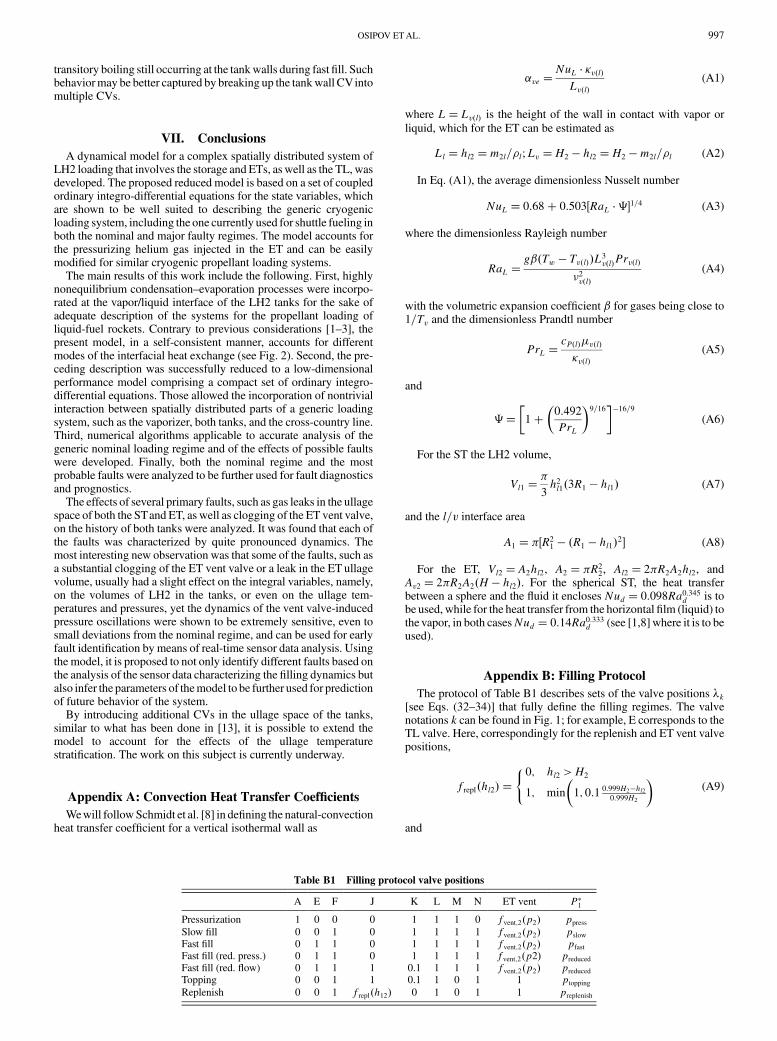
Appendix B: Filling ProtocolThe protocol of Table B1 describes sets of the valve positions $k

[see Eqs. (32–34)] that fully define the filling regimes. The valvenotations k can be found in Fig. 1; for example, E corresponds to theTL valve. Here, correspondingly for the replenish and ET vent valvepositions,

frepl!hl2" $( 0; hl2 >H2

1; min

#1; 0:1 0:999H2%hl2

0:999H2

$(A9)

and

Table B1 Filling protocol valve positions

A E F J K L M N ET vent P/1

Pressurization 1 0 0 0 1 1 1 0 fvent;2!p2" ppress

Slow fill 0 0 1 0 1 1 1 1 fvent;2!p2" pslow

Fast fill 0 1 1 0 1 1 1 1 fvent;2!p2" pfast

Fast fill (red. press.) 0 1 1 0 1 1 1 1 fvent;2!p2" preduced

Fast fill (red. flow) 0 1 1 1 0.1 1 1 1 fvent;2!p2" preduced

Topping 0 0 1 1 0.1 1 0 1 1 ptopping

Replenish 0 0 1 frepl!h12" 0 1 0 1 1 preplenish

OSIPOV ETAL. 997

fvent;2!p2" $

8<:

0; p2 % p2;low

1; p2 % p2;high

$%vent;2; otherwise(A10)

where $%k refers to the previous value of $.For the ST vent and vaporizer valves, the vent positions $ are

described correspondingly by

fvap!p1; p/1"

$

8<:

min !1;maxf0; 10+!p/1 % p1"= % p/1 ,g"; p1 < 0:98p/10; p1 > 1:02p/1$%vap; otherwise

(A11)

and

fvent;1!p1; p/1" $

(0; p1 < 1:05p/11; p1 > 0:95p/1$%vent; otherwise

(A12)

Here, p/1 refers to desired values of pressure in the ST that arespecified in the last column of the Table B1.

Appendix C: Simulation Parameter ValuesSimulation parameter values are given in Table C1. Many of the

system parameters values were derived directly from systemdocuments. The remaining parameters were estimated from systemdata, including )vap, cvap, !l;e, )tr, and each of the Kk values fork 2 fE;F; J; K; L;M;Ng (see Fig. 1). The position of the main fillvalve K in its reduced-flow state during fast fill (reduced flow) andtopping was also estimated from data.

References[1] Estey, P. N., Lewis, D. H., Jr., and Connor, M., “Prediction of a

Propellant Tank Pressure History Using State SpaceMethods,” Journalof Spacecraft and Rockets, Vol. 20, No. 1, 1983, pp. 49–54.doi:10.2514/3.28355

[2] Torre, C. N., Witham, J. A., Dennison, E. A., McCool, R. C., andRinker, M. W., “Analysis of a Low-Vapor-Pressure CryogenicPropellant Tankage System,” Journal of Spacecraft and Rockets,

Vol. 26, 1989, pp. 368–378.doi:10.2514/3.26081

[3] DeFelice, D. M., and Aydelott, J. C., “Thermodynamic Analysis andSubscale Modeling of Space-Based Cryogenic Propellant Systems,”NASATM-8992, July 1987.

[4] Osipov, V. V., andMuratov, C. B., “Dynamic Condensation Blocking inCryogenic Refueling,” Applied Physics Letters, Vol. 93, No. 22, 2008,Paper 224105.doi:10.1063/1.3025674

[5] Landau, L. D., and Lifshitz, E.M.,FluidMechanics, 2nd ed., PergamonPress, New York, 1987, p. 203.

[6] Clark, J. A., “Universal Equations for Saturation Vapor Pressure,” 40thAIAA/ASME/SAE/ASEE Joint Propulsion Conference and Exhibit,Fort Lauderdale, FL, AIAA Paper 2004-4088, July 2004.

[7] Dean, J. A., Lange’s Handbook of Chemistry, 12th ed., McGraw–Hill,New York, 1979, pp. 5.30, 6.129.

[8] Schmidt, F. W., Henderson, R. E., and Wolgemuth, C. H., Introductionto Thermal Sciences, 2nd ed., Wiley, New York, 1993, pp. 179, 240.

[9] Osipov, V. V., Luchinsky, D.G., Smelyanskiy, V. N., Kiris, C., Timucin,D. A., and Lee, S. H., “In-Flight Failure Decision and Prognostic for theSolid Rocket Booster,” 43rd AIAA/ASME/SAE/ ASEE JointPropulsionConference andExhibit, Cincinnati, OH,AIAAPaper 2007-582, July 2007.

[10] Streeter, V. L., Wylie, E. B., and Bedford, K. W., Fluid Mechanics,9th ed., McGraw–Hill, New York, 1998, p. 421.

[11] Daigle, M., and Goebel, K., “Model-Based Prognostics Under LimitedSensing,” Proceedings of the 2010 IEEE Aerospace Conference[online], IEEE Publ., Piscataway, NJ, March 2010.doi:10.1109/AERO.2010.5446822

[12] Ahuja, V., Hosagady, A., Mattick, S., Lee, C. P., Field, R. E., and Ryan,H., “Computational Analyses of Pressurization in Cryogenic Tanks,”44th AIAA/ASME/SAE/ASEE Joint Propulsion Conference andExhibit, Hartford, CT, AIAA Paper 2008-4752, July 2008.

[13] Schallhorn, P., Campbell, D. M., Chase, S., Puquero, J., Fontenberry,C., Li, X., andGrob, L., “Upper Stage TankThermodynamicModellingUsing SINDA/FLUINT,” 42nd AIAA/ASME/SAE/ASEE JointPropulsion Conference and Exhibit, Sacramento, CA, AIAAPaper 2006-5051, July 2006.

[14] Grayson, G., Lopez, A., Chandler, F., Hastings, L., Hedayat, A., andBrethour, J., “CDF Modelling of Helium Pressurant Effects onCryogenic Tank Pressure Rise Rates in Normal Gravity,” 43rd AIAA/ASME/SAE/ASEE Joint Propulsion Conference and Exhibit,Cincinnati, OH, AIAA Paper 2007-5524, July 2007.

T. LinAssociate Editor

Table C1 Parameter values

Component Parameter values

Hydrogen andhelium

Tc $ 33:2 K, pc $ 1:315 * 106 Pa, $$ 5, 'L $ 71:1 kg=m3, cL $ 9450 J=kg=K, #L $ 0:0984 W=m=K, h0lv $ 4:47 * 105 J=kg,%$ 3:4 * 10%6 Pa # s, Rv $ 4124 J=kg=K, cV;v $ 6490 J=kg=K, " $ 5=3, #v $ 0:0166 W=m=K, Rg $ 2077 J=kg=K,

#g $ 0:0262 W=m=K, cV;g $ 3121 J=kg=K, cP;g $ 5193 J=kg=KST R1 $ 9:16 m, )vap $ 20 s, cvap $ 5:89 * 10%4, Svalve;1 $ 0:025 m2

ET R2 $ 4:02 m, H2 $ 26:96 m2, !l;e $ 8:0 W=m2=K, mwcw $ 5 * 105 J=K, Svalve;2 $ 0:05 m2

TL Dpipe $ 0:254 m, lpipe $ 457:2 m, dr $ 1 * 10%6, )tr $ 10 s, SE $ 0:1013 m2, KE $ 4, SF $ 0:1459 m2, KF $ 1 * 105,SJ $ 0:0041 m2, KJ $ 66, SK $ 0:0643 m2, KK $ 140, SL $ 0:0643 m2, KL $ 0:11, SM $ 0:0643 m2, KM $ 0:11,

SN $ 0:0643 m2, KN $ 0:38

998 OSIPOV ETAL.