Dynamic Two-way Relationship between Exporting … CHAPTER 3 Dynamic Two-way Relationship between...

Chapter 3

Dynamic Two-way Relationship between Exporting and

Importing: Evidence from Japan

Kazunobu Hayakawa

Bangkok Research Center, Institute of Developing Economies, Thailand

Toshiyuki Matsuura

Institute for Economic and Industrial Studies, Keio University, Japan

May 2016

This chapter should be cited as

Hayakawa, K. And T. Matsuura (2014), ‘Dynamic Two-way Relationship between

Exporting and Importing: Evidence from Japan, Hahn, C.H. and D. Narjoko (eds.),

‘Globalization and Performance of Small and Large Firms. ERIA Research Project

Report 2013-3, pp.III-1-III-28, Available at:

ww.eria.org/RPR_FY2013_No.3_Chapter_13.pdf

III-1

CHAPTER 3

Dynamic Two-way Relationship between Exporting and

Importing: Evidence from Japan1

KAZUNOBU HAYAKAWA

Bangkok Research Center, Institute of Developing Economies, Thailand

TOSHIYUKI MATSUURA#

Institute for Economic and Industrial Studies, Keio University, Japan

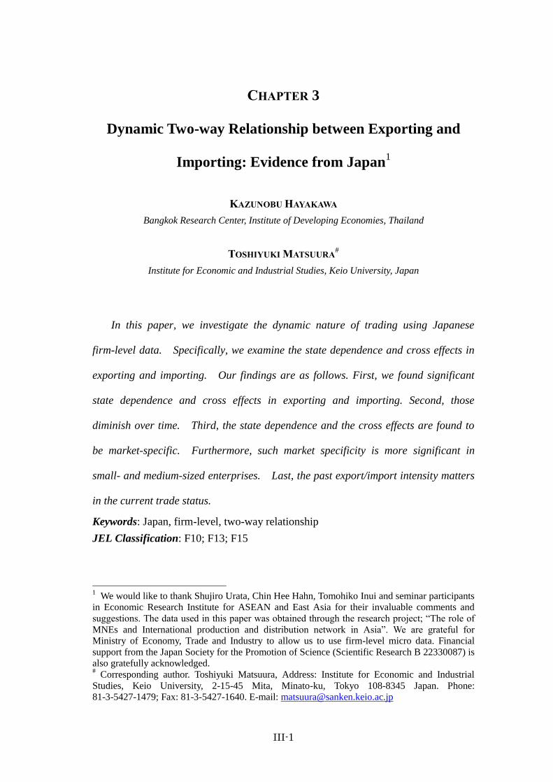
In this paper, we investigate the dynamic nature of trading using Japanese

firm-level data. Specifically, we examine the state dependence and cross effects in

exporting and importing. Our findings are as follows. First, we found significant

state dependence and cross effects in exporting and importing. Second, those

diminish over time. Third, the state dependence and the cross effects are found to

be market-specific. Furthermore, such market specificity is more significant in

small- and medium-sized enterprises. Last, the past export/import intensity matters

in the current trade status.

Keywords: Japan, firm-level, two-way relationship

JEL Classification: F10; F13; F15

1 We would like to thank Shujiro Urata, Chin Hee Hahn, Tomohiko Inui and seminar participants

in Economic Research Institute for ASEAN and East Asia for their invaluable comments and

suggestions. The data used in this paper was obtained through the research project; “The role of

MNEs and International production and distribution network in Asia”. We are grateful for

Ministry of Economy, Trade and Industry to allow us to use firm-level micro data. Financial

support from the Japan Society for the Promotion of Science (Scientific Research B 22330087) is

also gratefully acknowledged. # Corresponding author. Toshiyuki Matsuura, Address: Institute for Economic and Industrial

Studies, Keio University, 2-15-45 Mita, Minato-ku, Tokyo 108-8345 Japan. Phone:

81-3-5427-1479; Fax: 81-3-5427-1640. E-mail: [email protected]

mailto:[email protected]

III-2

1. Introduction

Recently, within-industry firm heterogeneity in terms of internationalization has

attracted many researchers’ attention. For example, larger-sized firms are in a more

advantageous position to gain the benefit from international activities such as

exporting and importing. Since the entry into foreign markets requires firms to bear

sunk costs, only productive firms, usually relatively large-sized enterprises (LEs) are

able to sell their products to foreign markets or to source intermediate goods from

foreign manufacturers. Especially, recent empirical studies (e.g., Vogel and Wagner,

2010) highlight that while most productive firms get engaged in both exporting and

importing, less productive firms, most of which are small- and medium-sized

enterprises (SMEs), become one-way traders or domestic firms. Namely, it is well

revealed in the literature that according to the differences in productivity or sizes,

there are various kinds of differences in firms’ international activities.

Another important aspect in firms’ international activities is the existence of their

dynamic nature. For example, once firms bear sunk costs for starting exporting,

they do not need to incur those costs in the following years and thus will be able to

easily continue their exporting activities. This is called “state dependence” in

exporting and has been empirically confirmed in several previous studies such as Das,

et al. (2007) and Roberts and Tybout (1997). The same story can be applied in the

context of importing. That is, firms with the past experience of importing will be

more likely to be importers in the future. Such state dependence in importing is also

found in Aristei, et al. (2013) and Muuls and Pisu (2009). However, the time

persistency of such state dependence might be controversial. Namely, while the

export experience one year ago has a positive effect on exporting in the current year,

III-3

the experience of last exporting in several years ago may not. Indeed, Roberts and

Tybout (1997) found that the state dependence persists until two years after exporting

and that the export experience in three years ago does not have significant effects on

exporting in the current year.

Furthermore, such a dynamic nature is expected to exist between exporting and

importing. As mentioned in Aristei, et al. (2013), common sunk costs arise when

firms implement an organizational structure in charge of international operations or

when firms acquire information on foreign markets, which may include both

potential buyers (export) and suppliers of intermediate inputs (import). Therefore,

the sunk costs for importing (exporting) will be lower for exporters (importers).

Also, even if there are no common sunk costs between exporting and importing,

productivity improvement through starting importing (exporting) may enable firms to

bear the original amount of sunk costs of exporting (importing). As a result, firms

with the past experience of exporting (importing) are expected to tend to start

importing (exporting) activities as well. This is called “cross effects” between

exporting and importing, which are empirically found in Aristei, et al. (2013),

Kasahara and Lapham (2013), and Muuls and Pisu (2009).


firm-level data. Specifically, we first examine whether state dependence and cross

effects exist in Japanese firms or not. Second, it is explored whether or not the

experience one year ago has different effects from that more than one years ago. This

analysis is similar to that in Roberts and Tybout (1997), but they do not examine such

time persistency for cross effects. Third, we also examine whether or not state

dependence and cross effects differ by firm characteristics such as firm size. Buono

and Fadinger (2012) examine the role of firm productivity (in addition to country

III-4

characteristics) in the state dependence in exporting but do not for that in importing

and cross effects. Last, we investigate whether state dependence and cross effects

are destination-specific or not. For example, it is examined whether or not the past

experience in exporting to Asia has the stronger effects in exporting to Asia in the

current year than the experience in exporting to other regions.

In addition to the above-mentioned self-selection into internationalization, the

literature has investigated the impacts of internationalization on firm productivity.2

For example, Wagner (2002) and De Loecker (2007) investigated exporters in

Germany and Slovenia, respectively, and found the positive impacts of exporting on

their productivity, i.e., learning-by-exporting. On the other hand, the results for the

impacts of importing are mixed. For example, Amiti and Konings (2007) found for

firms in Indonesia that the increase of imported inputs through tariff reduction

enhances firm productivity. However, Vogel and Wagner (2010) did not find the

learning-by-importing in Germany. One source for this different result is that while

imported inputs have much better quality than domestic inputs in the case of

developing countries, the difference in quality between imported and domestic inputs

is not so significant in the case of developed countries. Thus, starting importing

does not lead to the significant productivity enhancement in the case of developed

countries.

If learning-by-importing is not available in the case of developed countries, it

becomes more important to analyze the dynamic transition process of firm

internationalization for Japanese case, a case of a developed country. Even if direct

positive impacts on firm productivity are not available from importing, the existence

2 As for the survey papers on this field, see, for example, Hayakawa et al. (2012) and Wagner

(2012).

III-5

of such two-way relationship means that importing activities encourage firms to start

exporting and yield positive impacts on productivity through learning-by-exporting.

In other words, importing activities have not direct but indirect impacts on firm

productivity. Thus, our analysis for Japanese case will contribute to enhancing our

understanding on how firms particularly in developed countries obtain benefits from

internationalization. Also, this dynamic transition process of importing and exporting

activities will uncover why the gap in productivity between SMEs and LEs expands

over time.3 Namely, while the LEs starting only exporting enjoy immediately

productivity enhancement through learning-by-exporting, those starting just

importing also may enjoy productivity enhancement through starting exporting

subsequently. On the other hand, SMEs cannot enjoy such productivity

enhancement because they do not afford starting either exporting or importing.

The rest of this paper is organized as follows. The next section specifies our

theoretical framework on state dependence and cross effects. Section 3 provides our

empirical framework and data sources. After taking a brief look at trade status in

Japanese firms in Section 4, we report our estimation results in Section 5. Section 6

concludes on this paper.

2. Theoretical Framework

In this section, we discuss the mechanism of the dynamic transition process of

importing and exporting activities. In particular, we shed light on the state

dependence and the cross effects. While the state dependence is the positive

relationship between the current and past status of exporting/importing, the cross

3 See Figure A1 in Appendix.

III-6

effects are that the past experience in importing (exporting) raises the probability of

exporting (importing) at the current year. To make our discussion clearer, we

suppose that total fixed costs for trading consist of sunk costs and the fixed costs

relating to, for example, market uncertainty. The former costs are borne by firms

only when they start trading while firms need to pay the latter fixed costs every

time.4

The relationship between sunk costs for trading and firm productivity is crucial

not only in the mechanism of firms’ trading but also for the existence of state

dependence and cross effects in trading. The literature has examined the

mechanism of firms’ trading. Melitz (2003) is the theoretical pioneering study on the

selection mechanism in firms’ exporting. The selection mechanism in firms’

importing is examined in Kasahara and Lapham (2013). In either case, sunk costs

for exporting and importing play a crucial role in the selection mechanism of

exporting and importing, respectively. Those studies theoretically demonstrate that

firms with relatively high productivity get engaged in exporting (importing) because

the more productive firms have the larger operating profits from exporting

(importing) and thus can still obtain non-negative gross profit even if they incur sunk

costs for exporting (importing). Thus, since firms with the past experience of

exporting (importing) do not need to incur sunk costs anymore, such firms will be

able to continue exporting (importing) in the future.

Nevertheless, in reality, many exporters (importers) enter into and exit from

exporting (importing) multiple times. For example, as formalized in Blum et al.

(2013) and Eaton et al. (2011), fixed costs for trading and/or demand in foreign

4 The former and latter costs are respectively called “entry fee” and “maintenance cost” in

Baldwin and Krugman (1989), “entry cost” and “reentry cost” in Roberts and Tybout (1997), and

“start-up costs” and “fixed costs” in Das et al. (2007).

III-7

market might include stochastic components. Then, the large negative shocks for

the fixed costs and the demand may not enable even firms with the trade experience

to continue trading. Under this case, “learning” plays an important role in

encouraging firms to continue trading. As mentioned in the introductory section,

exporting and importing contributes to enhancing firms’ productivity through

learning advanced knowledge in the foreign market or enjoying economies of scale.

These are called learning-by-exporting and learning-by-importing though the

learning-by-importing may not be available in the case of firms in developed

countries. Also, as theoretically demonstrated in Albornoz, et al. (2012), Arkolakis

and Papageorgiou (2009), and Buono and Fadinger (2012), firms that start trading

learn about foreign market and thus may face the lower demand uncertainty from the

next year. As a result, with the rise of productivity through trading or the decrease

of market uncertainty, firms can obtain the larger benefits from trading and will be

likely to continue trading.

Also, the productivity rise through learning-by-exporting

(learning-by-importing) becomes one of the important sources for cross effects.

The productivity rise through exporting (importing) increases the benefits from

importing (exporting) and thus encourages firms to start importing (exporting). In

addition, the existence of the common fraction in sunk costs between exporting and

importing becomes another important source. The organizational division and

system for international business in addition to the general knowledge on

international business can be shared between exporting and importing. As a result,

cross effects between exporting and importing will work.

There are some more issues on state dependence and cross effects. The first is

their relationship with time. On the one hand, state dependence and cross effects may

III-8

diminish over time because the sunk costs for trading may recover to the original

amount over time. On the other hand, as theoretically formalized in Arkolakis and

Papageorgiou (2009), and Buono and Fadinger (2012), market uncertainty may

decrease over time. In addtion, as empirically found in De Loecker (2007), the rise of

productivity through trading increases over time. As a result, the relationship of

state dependence and cross effects with time is an empirical question.

Second, the magnitude of state dependence may differ by firm characteristics.

For example, the rise of productivity through trading differs by pre-trading

productivity or sizes. Lileeva and Trefler (2010) and Serti and Tomasi (2008) found

the larger productivity rise in low productive firms and medium- and large-sized

firms, respectively. In addition, low productive or small-sized firms may be likely to

stop trading. This stop might be because of knowing the real magnitude of demand

uncertainty by trying trading (Albornoz, et al., 2012) or of the small capacity of

production (i.e. small capital investments) (Blum, et al., 2013). Again, due to the

heterogeneous effects of trading on productivity across firms, the cross effects may

be different according to firm characteristics.

Third, the state dependence and the cross effects might be market-specific. The

sunk costs and fixed costs in addition to market uncertainty might have some

components specific to trading partner countries. In other words, even if having the

experience of bearing sunk costs in exporting to a region, firms may need to again

bear sunk costs in exporting to other regions. Furthermore, as shown in De Loecker

(2007), the effects of trading on productivity differ by partner country. He found

that the effects of exporting to high income countries on firm productivity are larger

than those of exporting to low income countries. Buono and Fadinger (2012) also

show the differences in the magnitude of state dependence according to partner

III-9

countries. As a result, the state dependence and the cross effects will be

market-specific to some extent.

3. Empirical Framework

In the literature, to analyze empirically the state dependence and cross effects for

exporting and importing, many previous papers such as Aristei, et al. (2013) estimate

a model for the probability of exporting or importing as a function of previous status

on both exporting and importing activities, in addition to several firm characteristics.

Then they estimate the bivariate probit model and investigate whether trading status

in previous period affects the current trading status. However, in this specification,

it is difficult to distinguish the cross effects toward two-way traders from those of

just switching between exporting and importing.

Instead, we use the category variable Yit which takes 0 for no trading firms, 1 for

export-only firms, 2 for import-only firms, and 3 for two-way-trading firms as a

dependent variable and then estimate multinomial logit model by employing the

following specification;

Prob(𝑌𝑖𝑡 = 𝑗) =exp(𝛼𝑖𝑗+𝐃𝑖,𝑡−1𝛃𝑖𝑗+𝐗𝑖,𝑡−1𝛄𝑖𝑗)

∑ exp(𝛼𝑖𝑘+𝐃𝑖,𝑡−1𝛃𝑖𝑘+𝐗𝑖,𝑡−1𝛄𝑖𝑘)𝑘,

where Di,t-1 is a vector of dummy variables on firm i’s status of internationalization,

namely exporter, or importer in year t-1. αij represents choice specific random effects,

which are unobserved firm heteronegeneity in total fixed costs for firm i. Xi,t-1

represents several firm characteristics, listed later. In our estimation strategy, firms

are assumed to decide whether they engage in only export, only import, or both in

each period. This framework is consistent with the decision for internationalization

discussed in Kasahara and Lapham (2013).

III-10

Following Todo (2011), to incorporate the correlation between random effects,

we allow random variation in a vector of coefficients for the lagged status variables,

βij, and estimate so-called random effect mixed logit model. One of the advantages

in using this specification lies in the relaxation of the interdependence from

irrelevant alternative (IIA) assumption. The standard multinomial logit model

assumes that the estimated coefficients are not changed even if we exclude one

choice from the choice set due to the IIA assumption. However, it is known that

this assumption is not always satisfied. Introducing random effects enables us to

relax this assumption and obtain more reliable estimation results.

Our firm-level control variables include the average wage rates (Wage), the share

of manufacturing workers in total workers (Share of Manu. Workers), the ratio of

R&D to total sales (R&D-Sales Ratio), debt-asset ratio (Debt-Asset Ratio), and total

factor productivity (TFP). We also introduce two Scale dummy variables. Scale

(301-999) takes the value one if a firm has more than 300 and less than 1,000

employees and zero otherwise. Scale (>999) does the value one if a firm has over

1,000 employees. Thus, SMEs, which have less than 300 employees, have the

value zero for these two Scale variables. This definition of SMEs is suggested by

Small and Medium Enterprise Basic Law in Japan. In this paper, we obtain TFP by

estimating production function with the Wooldridge (2009) modification of the

Levinshon and Petrin (WLP). This method takes into account the potential

collineality issue in the first stage of Levinshon and Petrin (2003) estimator

suggested by Ackerberg, et al. (2006). We also include industry dummy and year

dummy variables. All independent variables are lagged for one year.

Data for Japan are drawn from the confidential micro database of the Kigyou

Katsudou Kihon Chousa Houkokusho (Basic Survey of Japanese Business Structure

III-11

and Activities: BSJBSA) prepared annually by the Research and Statistics

Department, the Ministry of Trade, Economy and Industry (METI) (1994-2009).

This survey was first conducted in 1991 and then annually from 1994. The main

purpose of the survey is to capture statistically the overall picture of Japanese

corporate firms in light of their activity diversification, globalization and strategies

on research and development and information technology.

The strength of this survey is the sample coverage and reliability of information.

It is compulsory for firms with more than 50 employees and with capital of more

than 30 million yen in manufacturing and nonmanufacturing firms (some

non-manufacturing industries such as construction, medical services and

transportation services are not included). Another advantage lies in the rich

information on global engagement, such as exporting, importing, outsourcing, and

foreign direct investment. One limitation is that some information on financial and

institutional features is not available. In 2002, the BSJBSA covered about one-third

of Japan’s total labour force excluding the public, financial and other services

industries that are not covered in the survey (Kiyota, Nakajima, and Nishimura,

2009).

Our sample selection policy is as follows; first, we focus on manufacturing

industry in this paper, although this survey covers non-manufacturing industries as

well as manufacturing firms. This is because the coverage of non-manufacturing

industry differs by years and is thus not consistent across years. Second, we restrict

our sample period to that from 1994 to 2009 and exclude sample firms that appear in

this survey only at once or twice since our estimation method, a dynamic

random-effects multinomial logit model requires sample firms to appear in at least

three consecutive years. Finally, basic statistics in our sample are reported in Table 1.

III-12

Table 1. Basic Statistics

N Mean S.D. p10 p90

Status 165,555 0.830 1.197 0.000 3.000

Export (t−1) 165,555 0.294 0.456 0.000 1.000

Export (t−2) 144,031 0.296 0.456 0.000 1.000

Export (t−3) 127,330 0.297 0.457 0.000 1.000

Export (t−4) 112,934 0.297 0.457 0.000 1.000

Export (t−5) 99,609 0.298 0.457 0.000 1.000

Export (t−1) * SME 165,555 0.199 0.400 0.000 1.000

Export (t−2) * SME 144,031 0.198 0.399 0.000 1.000

Export (t−3) * SME 127,330 0.197 0.398 0.000 1.000

Export (t−4) * SME 112,934 0.196 0.397 0.000 1.000

Export (t−5) * SME 99,609 0.195 0.396 0.000 1.000

Import (t−1) 165,555 0.260 0.439 0.000 1.000

Import (t−2) 144,031 0.260 0.439 0.000 1.000

Import (t−3) 127,330 0.259 0.438 0.000 1.000

Import (t−4) 112,934 0.258 0.437 0.000 1.000

Import (t−5) 99,609 0.255 0.436 0.000 1.000

Import (t−1) * SME 165,555 0.180 0.384 0.000 1.000

Import (t−2) * SME 144,031 0.177 0.382 0.000 1.000

Import (t−3) * SME 127,330 0.175 0.380 0.000 1.000

Import (t−4) * SME 112,934 0.172 0.378 0.000 1.000

Import (t−5) * SME 99,609 0.169 0.375 0.000 1.000

SME 165,555 0.846 0.361 0.000 1.000

ln TFP 165,555 2.995 0.760 2.111 3.920

ln Wage 165,555 1.548 0.389 1.080 1.984

R&D-Sales Ratio 165,555 0.010 0.029 0.000 0.032

Debt-Asset Ratio 165,555 0.681 0.281 0.322 0.945

Share of Manu. Workers 165,555 0.654 0.258 0.271 0.932

Scale (301-999) 165,555 0.180 0.384 0.000 1.000

Scale (>999) 165,555 0.064 0.244 0.000 0.000

Export Share (t−1) 163,740 0.037 0.109 0.000 0.111

Export Share (t−1) * SME 163,740 0.022 0.085 0.000 0.044

Import Share (t−1) 163,740 0.037 0.125 0.000 0.089

Import Share (t−1) * SME 163,740 0.027 0.110 0.000 0.041

Source: Authors’ calculation

4. Data Overview

Before moving estimation results, we take a brief look at firms’ trade status.

Table 2 reports the share of the number of firms categorized into each status, in total

number of firms. The status includes no trade (Domestic), only exporting (Export),

III-13

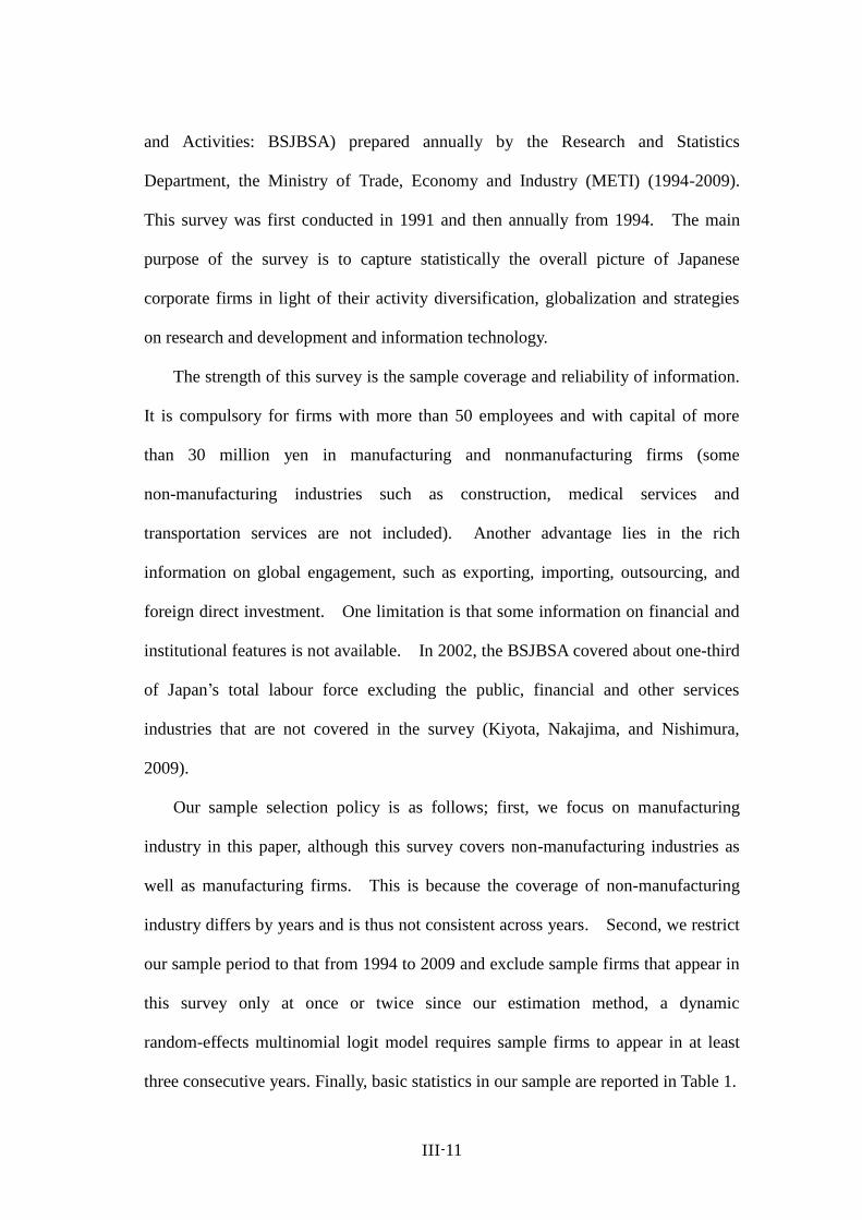
only importing (Import), and both exporting and importing (Two-way). The table

shows the highest share in “Domestic”, followed by “Two-way”. It is interesting

that the share of “Two-way” is higher than that of “Export” or that of “Import”. In

other words, a larger number of firms get engaged in both exporting and importing

than in either exporting or importing. The table also shows the stable shares of

“Export” (around 11%) and “Import” (around 8%) over time. On the other hand,

while the share of “Domestic” declines steadily from 67% in 1994 to 59% in 2009,

that of “Two-way” rises from 14% to 22%.

Table 2. Shares according to Trade Status

Domestic Export Import Two-way

1994 67% 11% 8% 14%

1995 65% 12% 8% 15%

1996 64% 11% 8% 16%

1997 67% 10% 8% 15%

1998 68% 10% 7% 15%

1999 67% 11% 7% 16%

2000 65% 11% 6% 18%

2001 64% 11% 7% 19%

2002 63% 11% 7% 20%

2003 61% 11% 8% 20%

2004 60% 11% 8% 21%

2005 60% 11% 8% 22%

2006 60% 11% 8% 22%

2007 59% 11% 9% 22%

2008 60% 11% 7% 22%

2009 59% 12% 7% 22%


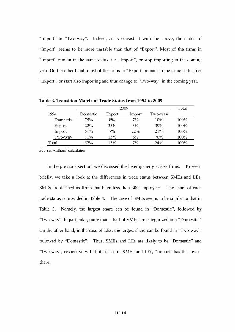
Next, Table 3 reports the transition matrices of trade status between 1994 and

2009. Most of the firms in each status keep the same status between two years. One

exception is the firms who got engaged in only importing in 1994. The majority of

those turned out to stop importing in 2009. Also, we can see that the share of firms

changing from “Export” to “Two-way” is higher than that of those changing from

III-14

“Import” to “Two-way”. Indeed, as is consistent with the above, the status of

“Import” seems to be more unstable than that of “Export”. Most of the firms in

“Import” remain in the same status, i.e. “Import”, or stop importing in the coming

year. On the other hand, most of the firms in “Export” remain in the same status, i.e.

“Export”, or start also importing and thus change to “Two-way” in the coming year.

Table 3. Transition Matrix of Trade Status from 1994 to 2009

Total


Domestic 75% 8% 7% 10% 100%

Export 22% 35% 3% 39% 100%

Import 51% 7% 22% 21% 100%

Two-way 11% 13% 6% 70% 100%

Total 57% 13% 7% 24% 100%

2009

1994


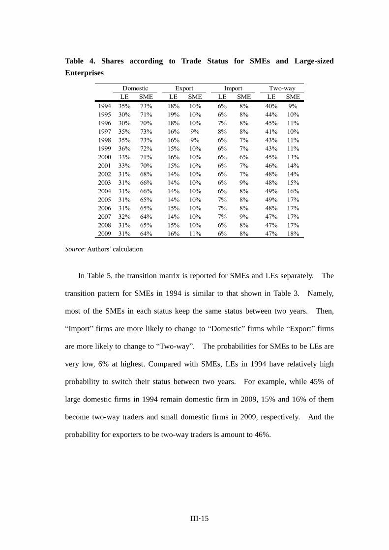
In the previous section, we discussed the heterogeneity across firms. To see it

briefly, we take a look at the differences in trade status between SMEs and LEs.

SMEs are defined as firms that have less than 300 employees. The share of each

trade status is provided in Table 4. The case of SMEs seems to be similar to that in

Table 2. Namely, the largest share can be found in “Domestic”, followed by

“Two-way”. In particular, more than a half of SMEs are categorized into “Domestic”.

On the other hand, in the case of LEs, the largest share can be found in “Two-way”,

followed by “Domestic”. Thus, SMEs and LEs are likely to be “Domestic” and

“Two-way”, respectively. In both cases of SMEs and LEs, “Import” has the lowest

share.

III-15

Table 4. Shares according to Trade Status for SMEs and Large-sized

Enterprises

LE SME LE SME LE SME LE SME

1994 35% 73% 18% 10% 6% 8% 40% 9%

1995 30% 71% 19% 10% 6% 8% 44% 10%

1996 30% 70% 18% 10% 7% 8% 45% 11%

1997 35% 73% 16% 9% 8% 8% 41% 10%

1998 35% 73% 16% 9% 6% 7% 43% 11%

1999 36% 72% 15% 10% 6% 7% 43% 11%

2000 33% 71% 16% 10% 6% 6% 45% 13%

2001 33% 70% 15% 10% 6% 7% 46% 14%

2002 31% 68% 14% 10% 6% 7% 48% 14%

2003 31% 66% 14% 10% 6% 9% 48% 15%

2004 31% 66% 14% 10% 6% 8% 49% 16%

2005 31% 65% 14% 10% 7% 8% 49% 17%

2006 31% 65% 15% 10% 7% 8% 48% 17%

2007 32% 64% 14% 10% 7% 9% 47% 17%

2008 31% 65% 15% 10% 6% 8% 47% 17%

2009 31% 64% 16% 11% 6% 8% 47% 18%



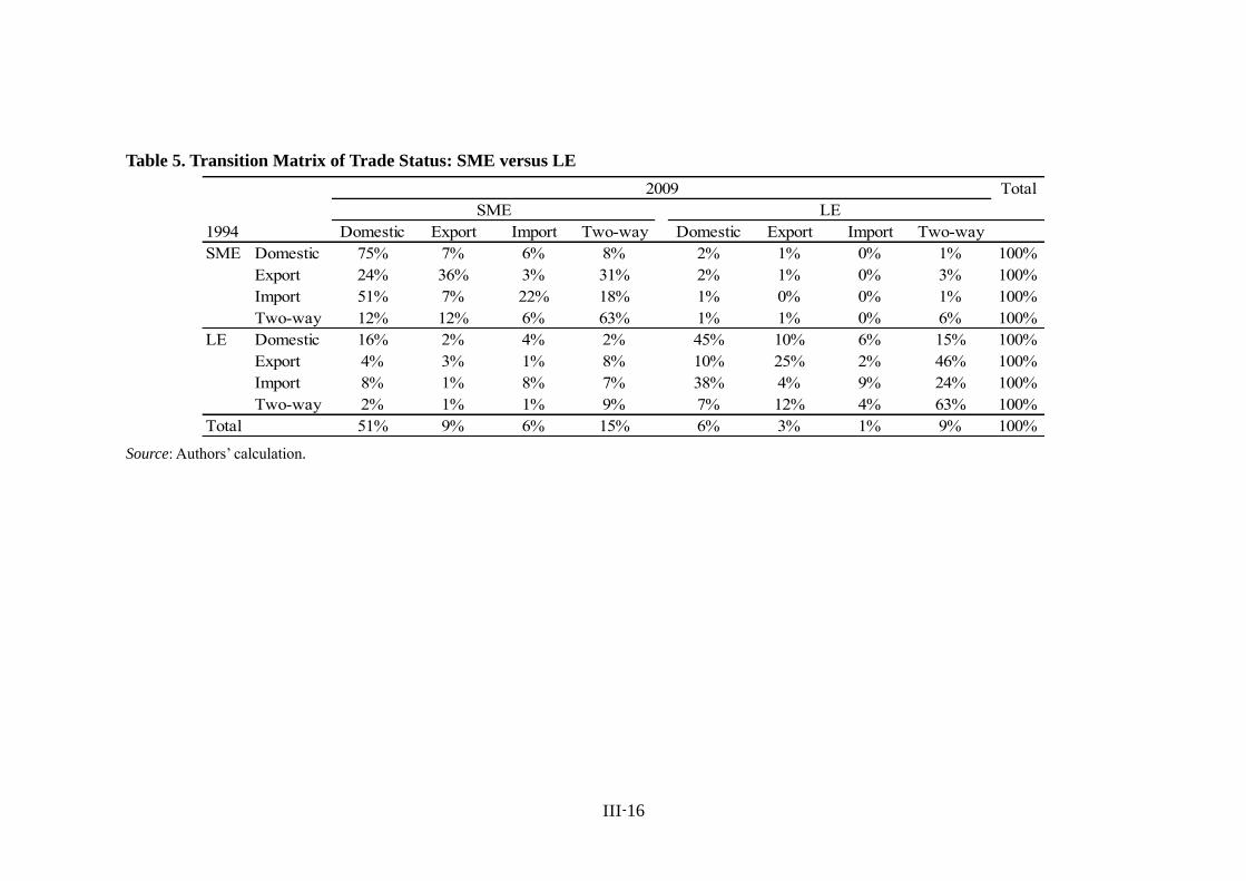
In Table 5, the transition matrix is reported for SMEs and LEs separately. The

transition pattern for SMEs in 1994 is similar to that shown in Table 3. Namely,

most of the SMEs in each status keep the same status between two years. Then,

“Import” firms are more likely to change to “Domestic” firms while “Export” firms

are more likely to change to “Two-way”. The probabilities for SMEs to be LEs are

very low, 6% at highest. Compared with SMEs, LEs in 1994 have relatively high

probability to switch their status between two years. For example, while 45% of

large domestic firms in 1994 remain domestic firm in 2009, 15% and 16% of them

become two-way traders and small domestic firms in 2009, respectively. And the

probability for exporters to be two-way traders is amount to 46%.

III-16

Table 5. Transition Matrix of Trade Status: SME versus LE

Total

1994 Domestic Export Import Two-way Domestic Export Import Two-way

SME Domestic 75% 7% 6% 8% 2% 1% 0% 1% 100%

Export 24% 36% 3% 31% 2% 1% 0% 3% 100%

Import 51% 7% 22% 18% 1% 0% 0% 1% 100%

Two-way 12% 12% 6% 63% 1% 1% 0% 6% 100%

LE Domestic 16% 2% 4% 2% 45% 10% 6% 15% 100%

Export 4% 3% 1% 8% 10% 25% 2% 46% 100%

Import 8% 1% 8% 7% 38% 4% 9% 24% 100%

Two-way 2% 1% 1% 9% 7% 12% 4% 63% 100%

Total 51% 9% 6% 15% 6% 3% 1% 9% 100%

LESME

2009

Source: Authors’ calculation.

III-17

Last, we take a brief look at how SMEs and LEs have different performance

indicators. Specifically, we examine three indicators including TFP, labor productivity,

and the ratio of R&D to sales. There are two important findings in Table 6. First, in all

indicators, LEs have the larger values/ratios than SMEs. Second, within each firm size

category, Two-way has the largest values/ratios, followed by Export, Import, and

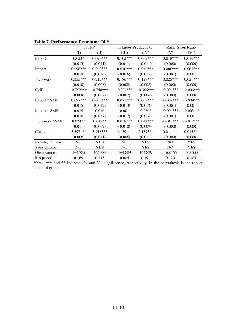
Domestic. We also compare these differences by regressing simple equations

(ordinary least squares, OLS). The results are reported in Table 7. Taking a look at

the specification with industry and year dummy variables, we can see the similar

differences with those confirmed in Table 6. One interesting finding in regression

analysis is that since the interaction term between export and SMEs has positive and

higher coefficients than that for export, exporter premium is larger within SMEs than

within LEs. All in all, these results suggest that total sunk costs are larger in order of

Two-way, Export, and Import.

Table 6. Performance Premium: Simple Average


ln TFP

SME 2.811 2.929 2.921 3.068

LE 3.557 3.574 3.668 3.791

ln Labor Productivity

SME 1.758 1.929 1.802 2.003

LE 2.124 2.214 2.179 2.303

R&D-Sales Ratio

SME 0.441 1.394 0.669 1.654

LE 1.06 2.895 1.735 3.504 Source: Authors’ calculation

III-18

Table 7. Performance Premium: OLS

(I) (II) (III) (IV) (V) (VI)

Export 0.023* 0.093*** 0.102*** 0.065*** 0.018*** 0.016***

(0.013) (0.011) (0.011) (0.011) (0.000) (0.000)

Import 0.098*** 0.060*** 0.046*** 0.040*** 0.006*** 0.005***

(0.019) (0.016) (0.016) (0.015) (0.001) (0.001)

Two-way 0.235*** 0.212*** 0.186*** 0.129*** 0.025*** 0.021***

(0.010) (0.008) (0.008) (0.008) (0.000) (0.000)

SME -0.759*** -0.748*** -0.371*** -0.366*** -0.006*** -0.006***

(0.008) (0.007) (0.007) (0.006) (0.000) (0.000)

Export * SME 0.097*** 0.055*** 0.071*** 0.055*** -0.009*** -0.009***

(0.015) (0.012) (0.013) (0.012) (0.001) (0.001)

Import * SME 0.019 0.016 0.001 0.026* -0.004*** -0.003***

(0.020) (0.017) (0.017) (0.016) (0.001) (0.001)

Two-way * SME 0.024** 0.019** 0.059*** 0.042*** -0.013*** -0.012***

(0.011) (0.009) (0.010) (0.009) (0.000) (0.000)

Constant 3.597*** 3.918*** 2.159*** 2.139*** 0.011*** 0.015***

(0.008) (0.011) (0.006) (0.011) (0.000) (0.000)

Industry dummy NO YES NO YES NO YES

Year dummy NO YES NO YES NO YES

Observations 164,785 164,785 164,889 164,889 165,555 165,555

R-squared 0.169 0.443 0.084 0.191 0.120 0.185

ln TFP ln Labor Productivity R&D-Sales Ratio

Notes: *** and ** indicate 1% and 5% significance, respectively. In the parenthesis is the robust

standard error.

III-19

5. Empirical Results

This section reports our estimation results. We first present our baseline estimation

results and then the results for some additional analyses.

5.1. Baseline Results

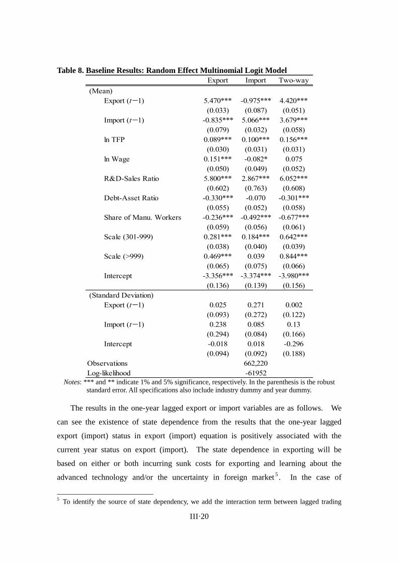
Our estimation results in the random effect multinomial logit model are reported in

Table 8. The results in firm characteristics are as follows. First, the highly

productive firms get engaged in exporting and/or importing. These results are well

known and are consistent with many previous papers including Aristei, et al. (2013) and

Muuls and Pisu (2009). Second, firms with the higher wages are more likely to get

engaged in exporting but are less likely to be engaged in importing. This symmetric

result is very interesting though it is difficult to interpret it well. In Muuls and Pisu

(2009), the coefficients for wage rates are estimated to be insignificant in both exporting

and importing. Third, taking a look at the results in Scale, we can see that SMEs are

less likely to get engaged in exporting, importing, and Two-way. It is interesting that

the effects of Scale (>999) on importing is insignificantly estimated. This result will

indicate that the very large-sized firms are more likely to get engaged in both exporting

and importing than in importing only. Fourth, the non-production worker-intensive

firms, R&D intensive firms, or firms with the less debt-asset ratio have the higher

probability of expiring and importing.

III-20

Table 8. Baseline Results: Random Effect Multinomial Logit Model

Export Import Two-way

(Mean)

Export (t−1) 5.470*** -0.975*** 4.420***

(0.033) (0.087) (0.051)

Import (t−1) -0.835*** 5.066*** 3.679***

(0.079) (0.032) (0.058)

ln TFP 0.089*** 0.100*** 0.156***

(0.030) (0.031) (0.031)

ln Wage 0.151*** -0.082* 0.075

(0.050) (0.049) (0.052)

R&D-Sales Ratio 5.800*** 2.867*** 6.052***

(0.602) (0.763) (0.608)

Debt-Asset Ratio -0.330*** -0.070 -0.301***

(0.055) (0.052) (0.058)

Share of Manu. Workers -0.236*** -0.492*** -0.677***

(0.059) (0.056) (0.061)

Scale (301-999) 0.281*** 0.184*** 0.642***

(0.038) (0.040) (0.039)

Scale (>999) 0.469*** 0.039 0.844***

(0.065) (0.075) (0.066)

Intercept -3.356*** -3.374*** -3.980***

(0.136) (0.139) (0.156)

(Standard Deviation)

Export (t−1) 0.025 0.271 0.002

(0.093) (0.272) (0.122)

Import (t−1) 0.238 0.085 0.13

(0.294) (0.084) (0.166)

Intercept -0.018 0.018 -0.296

(0.094) (0.092) (0.188)

Observations 662,220

Log-likelihood -61952 Notes: *** and ** indicate 1% and 5% significance, respectively. In the parenthesis is the robust

standard error. All specifications also include industry dummy and year dummy.

The results in the one-year lagged export or import variables are as follows. We

can see the existence of state dependence from the results that the one-year lagged

export (import) status in export (import) equation is positively associated with the

current year status on export (import). The state dependence in exporting will be

based on either or both incurring sunk costs for exporting and learning about the

advanced technology and/or the uncertainty in foreign market5. In the case of

5 To identify the source of state dependency, we add the interaction term between lagged trading

III-21

importing, taking into account the absence of learning-by-importing in developed

countries, we may say that it is sourced mainly from incurring sunk costs for importing.

On the other hand, while the lagged export (import) status in import (export) equation

has significantly negative coefficients, the results in two-way equation show the

significantly positive coefficients for both the lagged export and import variables.

These results imply that the cross effects toward two-way traders exist rather than those

encouraging switching between exporting and importing. The existence of cross

effects in not only exporting but also importing will show that the significant fraction of

sunk costs is common between exporting and importing.

From the results in standard deviations of coefficients, we can see that all of them

are insignificant, suggesting that coefficients do not vary by firm and by mode of

internationalization and that the results for multinomial logit model do not differ from

the random effect multinomial logit estimation so much. Therefore, we focus on the

results of multinomial logit model for further analysis. Indeed, the multinomial logit

model greatly saves the computation time, compared with the random effect

multinomial logit model.

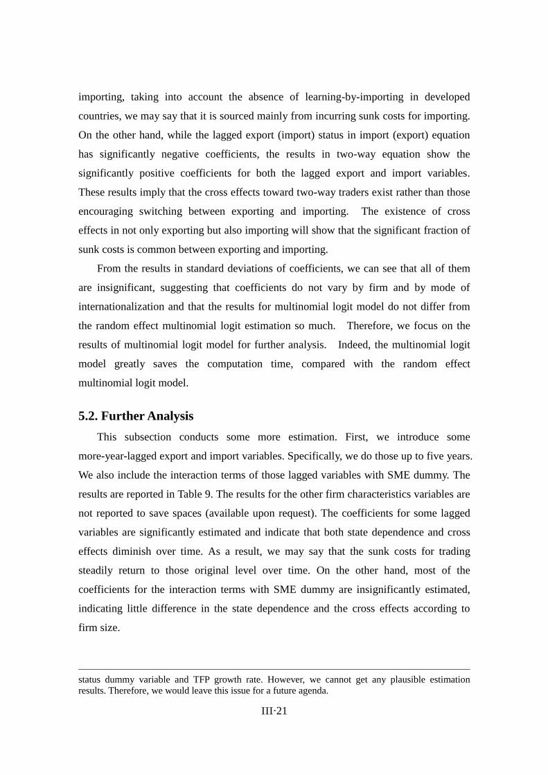
5.2. Further Analysis

This subsection conducts some more estimation. First, we introduce some

more-year-lagged export and import variables. Specifically, we do those up to five years.

We also include the interaction terms of those lagged variables with SME dummy. The

results are reported in Table 9. The results for the other firm characteristics variables are

not reported to save spaces (available upon request). The coefficients for some lagged

variables are significantly estimated and indicate that both state dependence and cross

effects diminish over time. As a result, we may say that the sunk costs for trading

steadily return to those original level over time. On the other hand, most of the

coefficients for the interaction terms with SME dummy are insignificantly estimated,

indicating little difference in the state dependence and the cross effects according to

firm size.

status dummy variable and TFP growth rate. However, we cannot get any plausible estimation

results. Therefore, we would leave this issue for a future agenda.

III-22

Table 9. Estimation Results: Further Lagged Variables


Export (t−1) 0.477*** -0.086*** 0.200***

(0.025) (0.006) (0.020)

Export (t−2) 0.081*** -0.027*** 0.064***

(0.018) (0.010) (0.018)

Export (t−3) 0.006 0.009 0.020

(0.015) (0.013) (0.017)

Export (t−4) 0.039** -0.009 0.014

(0.017) (0.012) (0.017)

Export (t−5) 0.046*** -0.023** 0.054***

(0.015) (0.009) (0.017)

Export (t−1) * SME -0.007 0.061*** 0.006

(0.011) (0.019) (0.013)

Export (t−2) * SME 0.007 0.009 0.017

(0.015) (0.014) (0.018)

Export (t−3) * SME 0.023 -0.020* 0.009

(0.019) (0.011) (0.019)

Export (t−4) * SME 0.001 0.001 0.004

(0.017) (0.014) (0.019)

Export (t−5) * SME -0.001 0.024 -0.001

(0.014) (0.015) (0.015)

Import (t−1) -0.100*** 0.411*** 0.224***

(0.006) (0.032) (0.025)

Import (t−2) -0.030*** 0.027** 0.048***

(0.012) (0.013) (0.018)

Import (t−3) -0.008 0.026* 0.013

(0.014) (0.014) (0.016)

Import (t−4) -0.014 0.020 0.022

(0.013) (0.014) (0.017)

Import (t−5) -0.021* 0.038*** 0.010

(0.011) (0.013) (0.013)

Import (t−1) * SME 0.033** -0.007 0.000

(0.017) (0.008) (0.013)

Import (t−2) * SME 0.008 0.031** 0.016

(0.016) (0.016) (0.017)

Import (t−3) * SME -0.010 -0.008 0.006

(0.015) (0.011) (0.018)

Import (t−4) * SME 0.006 -0.002 0.003

(0.017) (0.012) (0.017)

Import (t−5) * SME 0.010 -0.012 0.024

(0.015) (0.009) (0.017)

Observations 91,025


standard error. All specifications also include industry dummy and year dummy. The results in the

other firm-level variables are not reported in this table.

III-23

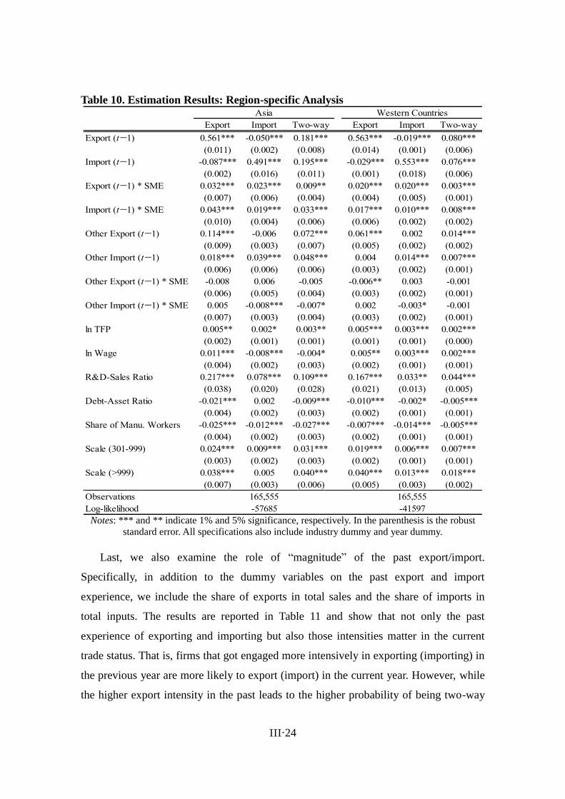
Next, we extend our model so as to capture the dimension of export destination and

import source countries. Namely, we investigate whether state dependence and cross

effects are market-specific or not. To this end, we define dependent variables and the

trade experience variables regionally. In particular, we examine trades with Asia and

Western countries (i.e. North American and European countries) separately.

Furthermore, in order to control for the role of the past experience of trade with the

other region, we also introduce the one-year lagged variables of the export and import

with the other region (Other Export and Other Import). The results are reported in Table

10. There are three noteworthy points. First, it shows the region-specific state

dependence and cross effects in both Asia and Western countries. Second, the

region-specific state dependence and cross effects are larger than the effects of the past

experience of trade with the other region. Third, the region-specific state dependence

and cross effects are larger in SMEs. Also, we have some evidence that trading with one

region discourages SMEs to start trading with the other region.

III-24

Table 10. Estimation Results: Region-specific Analysis

Export Import Two-way Export Import Two-way

Export (t−1) 0.561*** -0.050*** 0.181*** 0.563*** -0.019*** 0.080***

(0.011) (0.002) (0.008) (0.014) (0.001) (0.006)

Import (t−1) -0.087*** 0.491*** 0.195*** -0.029*** 0.553*** 0.076***

(0.002) (0.016) (0.011) (0.001) (0.018) (0.006)

Export (t−1) * SME 0.032*** 0.023*** 0.009** 0.020*** 0.020*** 0.003***

(0.007) (0.006) (0.004) (0.004) (0.005) (0.001)

Import (t−1) * SME 0.043*** 0.019*** 0.033*** 0.017*** 0.010*** 0.008***

(0.010) (0.004) (0.006) (0.006) (0.002) (0.002)

Other Export (t−1) 0.114*** -0.006 0.072*** 0.061*** 0.002 0.014***

(0.009) (0.003) (0.007) (0.005) (0.002) (0.002)

Other Import (t−1) 0.018*** 0.039*** 0.048*** 0.004 0.014*** 0.007***

(0.006) (0.006) (0.006) (0.003) (0.002) (0.001)

Other Export (t−1) * SME -0.008 0.006 -0.005 -0.006** 0.003 -0.001

(0.006) (0.005) (0.004) (0.003) (0.002) (0.001)

Other Import (t−1) * SME 0.005 -0.008*** -0.007* 0.002 -0.003* -0.001

(0.007) (0.003) (0.004) (0.003) (0.002) (0.001)

ln TFP 0.005** 0.002* 0.003** 0.005*** 0.003*** 0.002***

(0.002) (0.001) (0.001) (0.001) (0.001) (0.000)

ln Wage 0.011*** -0.008*** -0.004* 0.005** 0.003*** 0.002***

(0.004) (0.002) (0.003) (0.002) (0.001) (0.001)

R&D-Sales Ratio 0.217*** 0.078*** 0.109*** 0.167*** 0.033** 0.044***

(0.038) (0.020) (0.028) (0.021) (0.013) (0.005)

Debt-Asset Ratio -0.021*** 0.002 -0.009*** -0.010*** -0.002* -0.005***

(0.004) (0.002) (0.003) (0.002) (0.001) (0.001)

Share of Manu. Workers -0.025*** -0.012*** -0.027*** -0.007*** -0.014*** -0.005***

(0.004) (0.002) (0.003) (0.002) (0.001) (0.001)

Scale (301-999) 0.024*** 0.009*** 0.031*** 0.019*** 0.006*** 0.007***

(0.003) (0.002) (0.003) (0.002) (0.001) (0.001)

Scale (>999) 0.038*** 0.005 0.040*** 0.040*** 0.013*** 0.018***

(0.007) (0.003) (0.006) (0.005) (0.003) (0.002)

Observations 165,555 165,555

Log-likelihood -57685 -41597

Asia Western Countries

Notes: *** and ** indicate 1% and 5% significance, respectively. In the parenthesis is the robust


Last, we also examine the role of “magnitude” of the past export/import.

Specifically, in addition to the dummy variables on the past export and import

experience, we include the share of exports in total sales and the share of imports in

total inputs. The results are reported in Table 11 and show that not only the past

experience of exporting and importing but also those intensities matter in the current

trade status. That is, firms that got engaged more intensively in exporting (importing) in

the previous year are more likely to export (import) in the current year. However, while

the higher export intensity in the past leads to the higher probability of being two-way

III-25

traders, firms with the high import intensity in the past do not necessarily become

two-way traders. Based on these results, we may say that the past export intensity is a

more important determinant in the current trade status than the past import intensity. In

addition, we can see from the results of the interaction terms of these intensity variables

with SME dummy that the role of such intensities in the current trade status is not

different according to firm size.

Table 11. Estimation Results: Export/Import Share


Export (t−1) 0.552*** -0.073*** 0.248***

(0.010) (0.003) (0.009)

Export (t−1) * SME 0.009* 0.032*** 0.002

(0.006) (0.009) (0.006)

Export Share (t−1) 0.136*** -0.170*** 0.156***

(0.027) (0.044) (0.028)

Export Share (t−1) * SME -0.029 -0.022 -0.032

(0.029) (0.052) (0.031)

Import (t−1) -0.096*** 0.496*** 0.258***

(0.003) (0.015) (0.013)

Import (t−1) * SME 0.035*** 0.001 0.008

(0.010) (0.004) (0.007)

Import Share (t−1) -0.072** 0.045*** 0.019

(0.032) (0.014) (0.024)

Import Share (t−1) * SME -0.055 -0.007 0.037

(0.036) (0.015) (0.026)

ln TFP 0.005** 0.003** 0.008***

(0.002) (0.001) (0.002)

ln Wage 0.012*** -0.007*** 0.005

(0.004) (0.002) (0.004)

R&D-Sales Ratio 0.332*** 0.094*** 0.363***

(0.040) (0.034) (0.043)

Debt-Asset Ratio -0.023*** -0.002 -0.021***

(0.004) (0.003) (0.004)

Share of Manu. Workers -0.011*** -0.014*** -0.044***

(0.004) (0.003) (0.004)

Scale (301-999) 0.019*** 0.006*** 0.052***

(0.003) (0.002) (0.004)

Scale (>999) 0.038*** -0.000 0.073***

(0.007) (0.004) (0.009)

Observations 163,740



III-26

6. Summary and Policy Implications


firm-level data. Specifically, we examine the state dependence and cross effects in

exporting and importing. Our findings are as follows. First, we found significant state

dependence and cross effects in exporting and importing. Thus, even without any

positive effects of starting importing on productivity, importers will be able to achieve

productivity enhancement through inducing exporting. Second, those diminish over

time. If this result indicates that the sunk costs for trading steadily return to those

original level over time, it is important how firms maintain their know-how on trading

particularly during the non-trading period. Third, the state dependence and the cross

effects are found to be market-specific. This implies that it is more difficult to expand

trading partners than to continue trading with the existing partners. Furthermore, such

market-specific state dependence and cross effects are more significant in SMEs. We

also find that trading with one region discourages SMEs to start trading with the other

region. Last, the past export/import intensity matters in the current trade status.

The implication specific for SMEs in developed countries is as follows. Due to the

more significant market specificity in the state dependence and cross effects, it is more

difficult for SMEs to expand their trading partners. In the case of SMEs, trading with

one region can even discourage to doing with the other region. These facts immediately

imply that if firms can enjoy some amount of positive productivity effects from each

trading partner, SMEs can obtain only the fewer amount of positive effects from trading

than LEs. In other words, it is important for policy makers to encourage SMEs to

expand their trading partners. The policy support is usually available particularly for

starting trading for the first time. However, our claim is that it is important to support

not only the beginners but also the firms trading with just a few partners.

III-27

Appendix. Performance Gap between LEs and SMEs


Notes: The figure indicates the ratio of the average performance of SMEs to that of LEs.

References

Ackerberg, D., Caves, K., and Frazer, G., 2006, Structural Identification of Production

Function, MPRA paper, 38349.

Albornoz, F., Calvo Pardo, H., Coros, G., and Ornelas, E., 2012. Sequential Exporting,

Journal of International Economics, 88(1), 17-31.

Amiti, M. and Konings, J., 2007, Trade Liberalization, Intermediate Inputs, and

Productivity, American Economic Review, 97(5), 1611-1638.

Arkolakis, C. and Papageorgiou, T., 2009, Selection, Growth and Learning,

Mimeograph.

Aristei, D., Castellani, D., and Franco, C., 2013, Firms’ Exporting and Importing

Activities: Is There a Two-way Relationship?, Review of World Economics,

149(1), 55-84.

Baldwin, R., and Krugman, P., 1989, 1989, Persistent Trade Effects of Large Exchange

Rate Shocks, Quarterly Journal of Economics, 104(4), 635-54.

Blum, B., Claro, S., and Horstmann, I., 2013, Occasional and Perennial Exporters,

Journal of International Economics, 90(1), 65-74.

Buono, I. and Fadinger, H., 2012, The Micro-Dynamics of Exporting: Evidence from

French Firms, Temi di Discussione, Number 880.

0.7

0.8

0.9

1.0

1994 1995 1996 1997 1998 1999 2000 2001 2002 2003 2004 2005 2006 2007 2008 2009

Value Added per worker

TFP

III-28

Das, S., Roberts, M., and Tybout, J., 2007, Market Entry Costs, Producer Heterogeneity,

and Export Dynamics, Econometrica, 75(3), 837-873.

De Loecker, J., 2007, Do Exports Generate Higher Productivity? Evidence from

Slovenia, Journal of International Economics, 73(1): 69-98.

Eaton, J., Kortum, S., and Kramarz, F., 2011, An Anatomy of International Trade:

Evidence From French Firms, Econometrica, 79(5), 1453-1498.

Hayakawa, K., Kimura, F., and Machikita, T., 2012, Globalization and Productivity: A

Survey of Firm-level Analysis, Journal of Economic Surveys, 26(2): 332-350.

Kasahara, H. and Lapham, B., 2013, Productivity and the Decision to Import and

Export; Theory and Evidence, Journal of International Economics, 89(2),

297-316.

Kiyota, K., Nakajima, T., and Nishimura, K., 2009, Measurement of the Market Power

of Firms: The Japanese Case in the 1990s, Industrial and Corporate Change,

18(3), 381-414.

Levinsohn, J., Petrin, A., 2003. Estimating Production Functions Using Inputs to

Control for Unobservables, Review of Economics and Studies, (70), 317–341.

Lileeva, A. and Trefler, D., 2010, Improved Access to Foreign Markets Raises

Plant-Level Productivity... for Some Plants, Quarterly Journal of Economics,

125(3), 1051-1099.

Melitz, M., 2003, The Impact of Trade on Intra-industry Reallocations and Aggregate

Industry Productivity, Econometrica, 71(6), 1695-1725.

Muuls, M. and Pisu, M., 2009, Imports and Exports at the Level of the Firm: Evidence

from Belgium, The World Economy, 32(5), 692-734.

Roberts, M. and Tybout, J., 1997, The Decision to Export in Colombia: An Empirical

Model of Entry with Sunk Costs, American Economic Review, 87(4), 545-564.

Serti, F. and Tomasi, C., 2008, Self Selection and Post-entry Effects of Exports:

Evidence from Italian Manufacturing Firms, Review of World Economics, 144(4),

660–94.

Todo, Y., 2011, Quantitative Evaluation of Determinants of Export and FDI: Firm-Level

Evidence from Japan, The World Economy, 34(3), 355-381.

Vogel, A. and Wagner, J., 2010, Higher Productivity in Importing German

Manufacturing Firms: Self-selection, Learning from Importing, or Both?,

Review of World Economics, 145(4), 641-665.

Wagner, J., 2002, The Causal Effects of Exports on Firm Size and Labor Productivity:

First Evidence from a Matching Approach, Economics Letters, 77(2): 287-292.

Wagner, J., 2012, International Trade and Firm Performance: A Survey of Empirical

Studies since 2006, Review of World Economics, 148(2), 235-267.

Wooldridge, J. M., 2009, On Estimating Firm-Level Production Function Using Proxy

Variables to Control for Unobservables, Economic Letters, 104(3), 112-114.

Dynamic Two-way Relationship between Exporting … CHAPTER 3 Dynamic Two-way Relationship between...

Documents

Transcript of Dynamic Two-way Relationship between Exporting … CHAPTER 3 Dynamic Two-way Relationship between...